Numerical Evaluation of the Flow Quality of a Large-Scale Low-Speed Wind Tunnel via Steady CFD Simulation

Abstract

This study presents a full-scale steady CFD methodology for evaluating flow quality in a large-scale low-speed wind tunnel (8 m × 6 m test section, 130 m/s). The tunnel geometry is resolved at 1:1 scale, the damping screens and honeycomb are modeled as porous media, and results are validated against wind tunnel test data and the GJB 1179A-2012 acceptance criteria. The baseline configuration reproduces the axial static pressure gradient within the acceptance criterion but substantially overpredicts turbulence intensity, dynamic pressure coefficient, and both velocity direction deviation angles. Damping screens, modeled as porous jumps, provide the dominant correction, bringing all metrics within the acceptance limits. Adding honeycomb yields incremental improvement: porous zone modeling preserves or improves all metrics, whereas a porous jump representation pushes velocity direction deviations beyond the limit. Between RNG k-ε and SST k-ω, only turbulence intensity is closure-dependent, with RNG k-ε closer to experiment. At Ma ≈ 0.38, compressibility does not alter the flow quality assessment, confirming that incompressible assumption is sufficient. By replacing costly physical trials with a validated CFD workflow, these findings provide a practical, resource-efficient reference for the CFD-based evaluation, design, and retrofit of wind tunnel infrastructure that underpins renewable-energy and energy-efficiency research.

1. Introduction

Wind tunnels are essential tools in science and engineering because they provide controlled, repeatable, and measurable flow environments for aerodynamics research, model validation, mechanism identification, and design verification across a wide range of fields [1,2,3,4,5]. Their significance extends across multiple disciplines. In aerospace, wind tunnel testing continues to support the design of aircraft aerodynamics, studies in nonlinear aeroelasticity, and evaluation of flight-control systems [6,7]. In automotive engineering, it remains key to studying drag, stability, and vehicle-flow interactions [8,9]. In railway engineering, wind tunnels and related experiments play a vital role in studying train aerodynamics, crosswind effects, slipstreams, tunnel pressure waves, and operational safety [10,11]. In civil and environmental wind engineering, wind tunnels are crucial for analyzing wind-induced loads, aerodynamic control, and pedestrian-level wind environments [12,13,14,15,16]. In sustainable energy engineering, wind tunnels underpin the development and validation of wind-turbine aerodynamics and energy-efficient, low-drag designs on which renewable-energy and energy-efficiency research relies [17,18]. Their ongoing utilization across these disciplines confirms that wind tunnels remain indispensable research infrastructure, and that the quality of the airflow they produce directly determines the value of the data they generate.

The value of a wind tunnel is determined not by its dimensions or installed power but by the quality of the airflow it delivers to the test section. For a low-speed wind tunnel, the Chinese standard GJB 1179A-2012 [19] defines flow quality through metrics evaluated specifically in the test section: the axial static pressure gradient, turbulence intensity, dynamic pressure coefficient, and two velocity direction deviation angles. Owen and Owen [20] emphasized that tunnel performance should be assessed not from mean speed alone but from the combined behavior of turbulence level, velocity nonuniformity, and flow angularity. Moonen et al. [21] proposed explicit flow quality indicators and demonstrated that such metrics can be used to evaluate existing facilities, quantify the effects of design modifications, and support CFD-based tunnel analysis. The underlying principle is clear: if the test section flow quality does not meet the stipulated criteria, the aerodynamic data obtained from the facility may reflect deficiencies in the tunnel rather than the intrinsic behavior of the test object.

Computational fluid dynamics has become a valuable complement to wind tunnel testing for evaluating internal flow quality. CFD can reveal the flow development through the tunnel circuit, identify problematic sections, and support design or retrofit decisions prior to costly physical modifications. Beyond wind tunnel facilities themselves, CFD predictions validated directly against wind tunnel measurements have supported structural aerodynamic assessment, including wind loads on dome structures [22], while CFD simulation alone continues to inform sustainability-oriented urban and residential wind environment design [23]. More broadly, CFD combined with AI/ML surrogate modeling is increasingly applied to accelerate parameter-sensitivity studies in other computationally intensive engineering systems [24]. Previous studies have demonstrated the utility of CFD for low-speed wind tunnels, including numerical evaluation of test section flow quality, validation against measurements, and support for tunnel design [25,26,27,28,29,30]. However, these studies primarily concern smaller facilities or tunnels at the design stage, and the main objective in most cases is to reproduce the overall internal flow pattern rather than to reproduce the measured flow quality metrics in the test section of a large built facility. This leaves open a more demanding question: can a practical full-scale steady CFD model reproduce the flow quality measured in the test section of a large operational low-speed wind tunnel?

The challenge is compounded by the role of flow-conditioning devices. In large-scale closed-circuit wind tunnels, the test section flow quality is not controlled solely by the tunnel geometry. Damping screens and honeycomb structures installed upstream of the contraction section play a critical role in attenuating turbulence, improving velocity uniformity, and straightening the flow before it enters the test section. Burley and Harrington [31] showed that a honeycomb combined with fine-mesh damping screens produced the lowest turbulence intensity at the contraction entrance in the NASA Lewis altitude wind tunnel. Kulkarni et al. [32] demonstrated that CFD can reproduce the overall conditioning effect of honeycomb–screen combinations with reasonable agreement. Li et al. [33] experimentally confirmed that honeycomb improves wind tunnel flow quality, while Li et al. [34] showed through CFD that upstream flow development strongly influences the resulting test section flow. Santos et al. [35] showed that the insertion of damping screens in a wind tunnel significantly improved velocity profile uniformity and reduced turbulence intensity dispersion. These studies collectively establish that flow-conditioning devices are central to achieving acceptable flow quality in the test section. However, in a full-scale CFD model, these devices cannot be resolved explicitly without prohibitive computational cost. Their representation through porous media models is therefore necessary, but the choice of representation is not straightforward, because damping screens and honeycomb perform different physical functions and have fundamentally different geometric characteristics.

Accordingly, this study develops a practical full-scale steady-state CFD methodology to evaluate the flow quality in a large-scale low-speed wind tunnel. The tunnel structure and guide vanes are modeled explicitly at 1:1 scale, while the damping screens and honeycomb are represented using porous media models. The CFD predictions are compared against wind tunnel test data and the flow quality requirements in the standard GJB 1179A-2012. The study progresses systematically: a baseline configuration without flow-conditioning devices is examined first to determine the capabilities and limitations of the explicit geometry model. The influence of damping screens is then evaluated, followed by a comparison of two candidate honeycomb representations—porous jump and porous zone—to determine the preferred modeling approach. The sensitivity of the conclusions to the turbulence closure is assessed, and the validation of the incompressible flow assumption at a 130 m/s operating condition is examined through a dedicated compressibility comparison. This study aims to provide a practical reference for the CFD-based evaluation, design, or retrofit of comparable large-scale wind tunnel facilities. By reproducing the measured test-section flow quality without recourse to full physical trials, the methodology helps reduce the material and energy expenditure of constructing and retrofitting large test facilities, thereby supporting the resource-efficient development of the aerodynamic testing infrastructure that underpins energy-efficiency and renewable-energy research.

Relative to these prior studies [25,26,27,28,29,30], which primarily concern smaller-scale or design-stage facilities and generally aim to reproduce the overall internal flow pattern rather than the measured test-section flow quality, the present study contributes in three respects. First, the wind tunnel geometry is resolved at full scale (1:1) for an existing, in-service 130 m/s facility, rather than a scaled or as-designed model. Second, the influence of the flow-conditioning devices is decomposed configuration-by-configuration, isolating the individual contribution of the damping screens and two candidate honeycomb representations to each flow quality metric, rather than reporting only the outcome of a single, fully conditioned model. Third, the sensitivity of the resulting flow quality assessment to the turbulence closure and to the incompressible-flow assumption is examined explicitly against the same wind tunnel benchmark. Taken together, this approach allows the CFD methodology to be used not only to reproduce a measured flow quality outcome, but to attribute that outcome to specific, transferable modeling choices, which is of direct practical value for the CFD-based evaluation, design, or retrofit of comparable large-scale wind tunnel facilities.

2. Large Low-Speed Wind Tunnel Facility and Experimental Data

2.1. Overview of the Large Low-Speed Wind Tunnel Facility

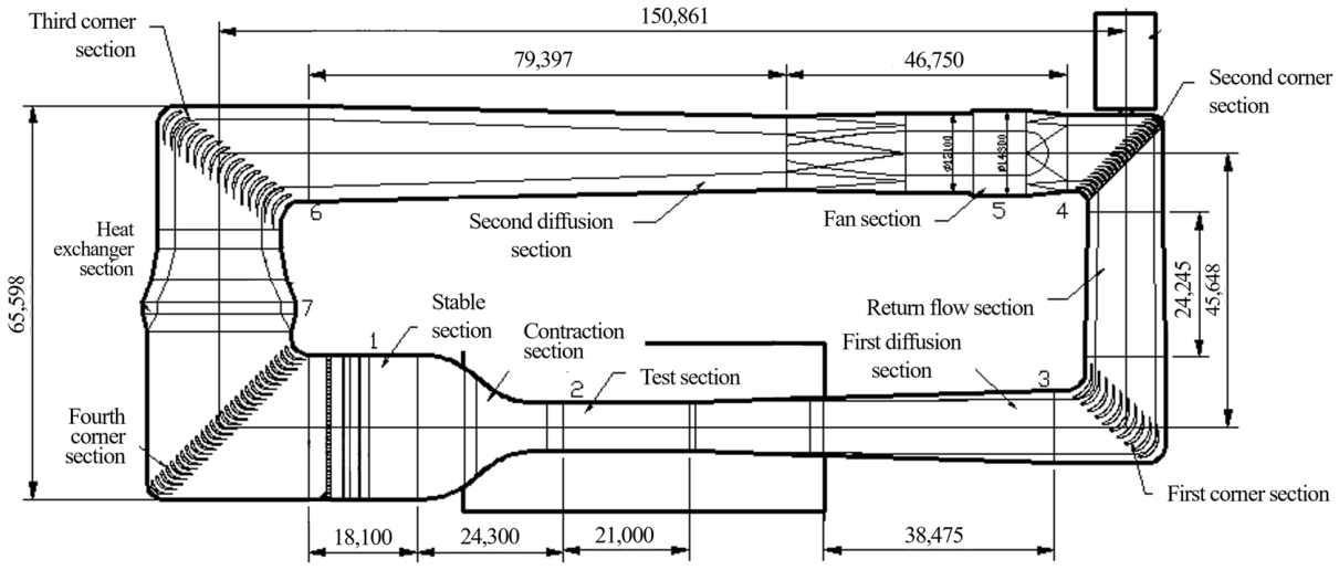
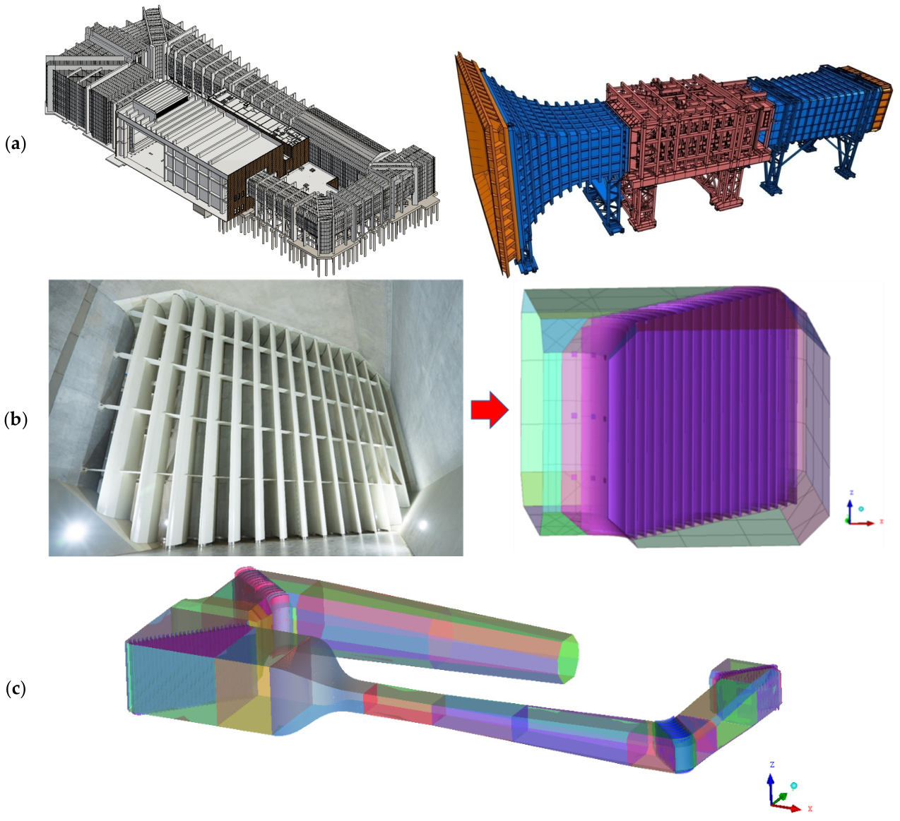
The Large Low-Speed Wind Tunnel is a large-scale closed-circuit facility for aerodynamic and acoustic testing. The tunnel circuit has a total axis length of 393 m. Starting from the fan section, the flow passes through the second diffusion section, the third and fourth corner sections, a heat exchanger section, the stable section, the contraction section, and into the test section. Downstream of the test section, the flow continues through the transition section, the first diffusion section, the return flow section, and the first and second corner sections before returning to the fan section. All corner sections are equipped with guiding vanes. The internal cross-sections are rectangular and octagonal. The test section is equipped with the dimensions of 8 m in width and 6 m in height, with a maximum operating wind speed of 130 m/s. Figure 1 shows the wind tunnel layout for this configuration.

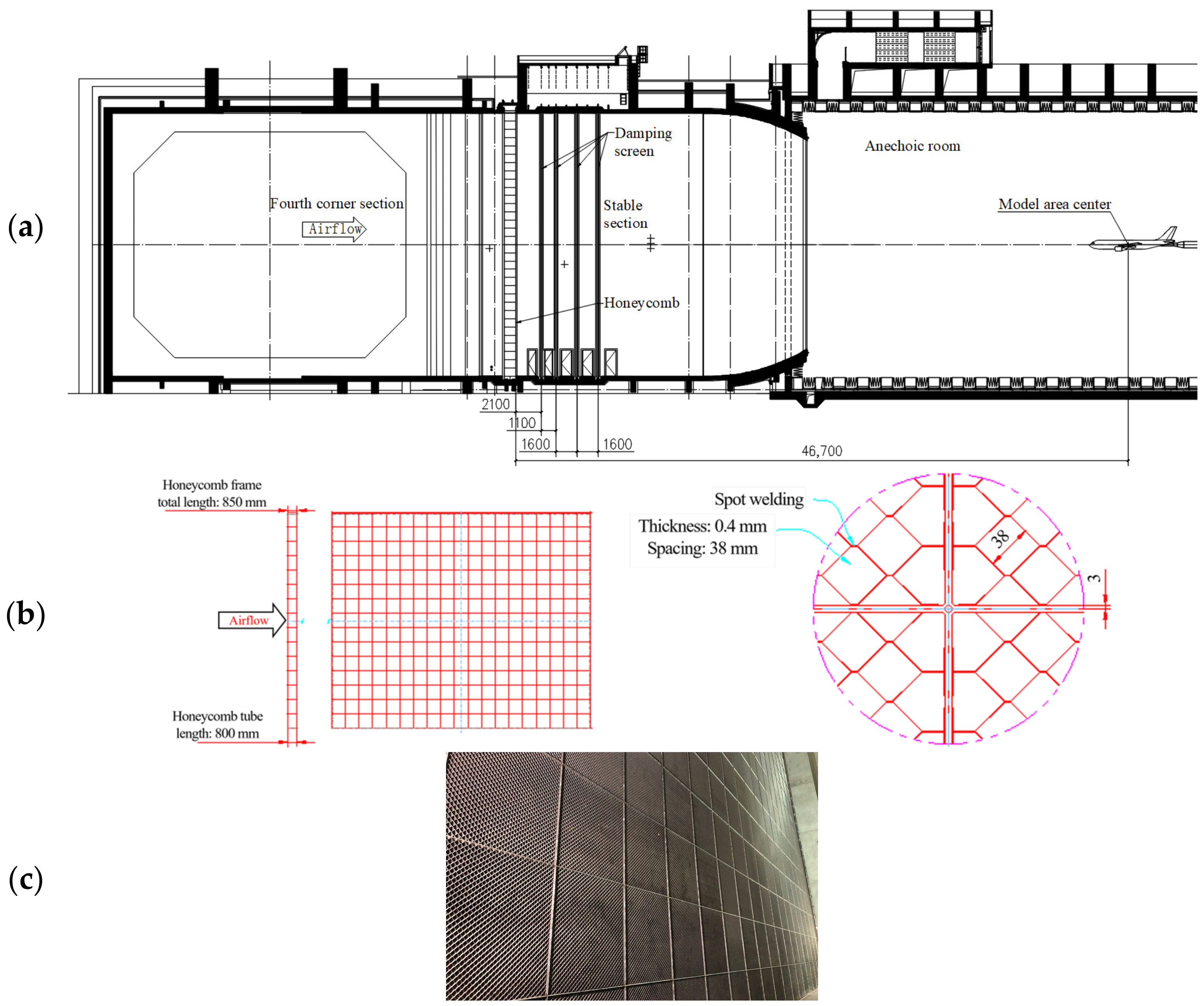
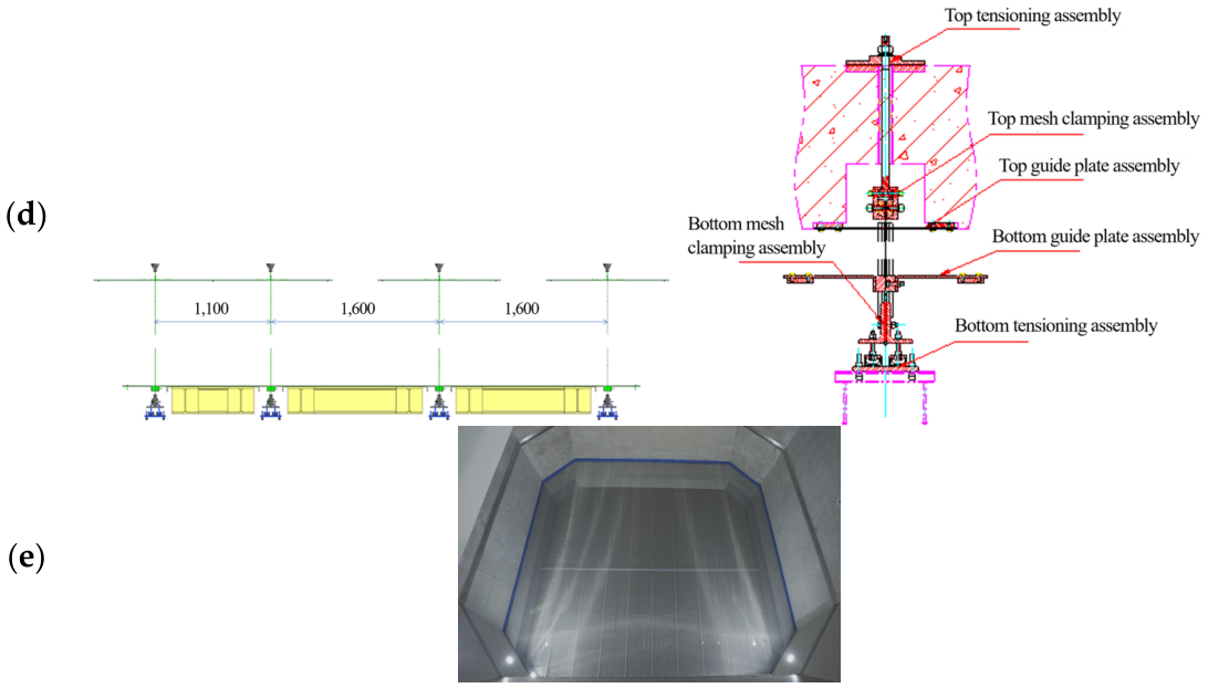
Flow conditioning in the Large Low-Speed Wind Tunnel is provided by a honeycomb layer and four layers of damping screens, all installed in the stable section upstream of the contraction section. The honeycomb is located 46.7 m upstream of the model area center, and the first damping screen layer is positioned 2.1 m downstream of the honeycomb. The honeycomb’s primary material is 304 stainless steel, with hexagonal cells having a diagonal spacing of 38 mm, a wall thickness of 0.4 mm, and a depth of 800 mm. The damping screen is constructed from steel wire with a diameter of 0.73 mm and a mesh size of 3.18 mm × 3.18 mm. The spacing between successive damping screens in the flow direction is 1.1 m, 1.6 m, and 1.6 m, respectively. Figure 2 illustrates the arrangement and installation of the flow-conditioning devices.

2.2. Flow Quality Metrics and Requirements

The flow quality in the test section is assessed using five evaluation metrics specified in the Chinese standard GJB 1179A-2012 [19]: axial static pressure gradient, turbulence intensity, dynamic pressure coefficient, and two velocity direction deviation angles. Together, these metrics provide a compact yet comprehensive characterization of the internal flow quality in terms of streamwise pressure development, residual turbulence level, velocity uniformity, and flow alignment with the tunnel axis.

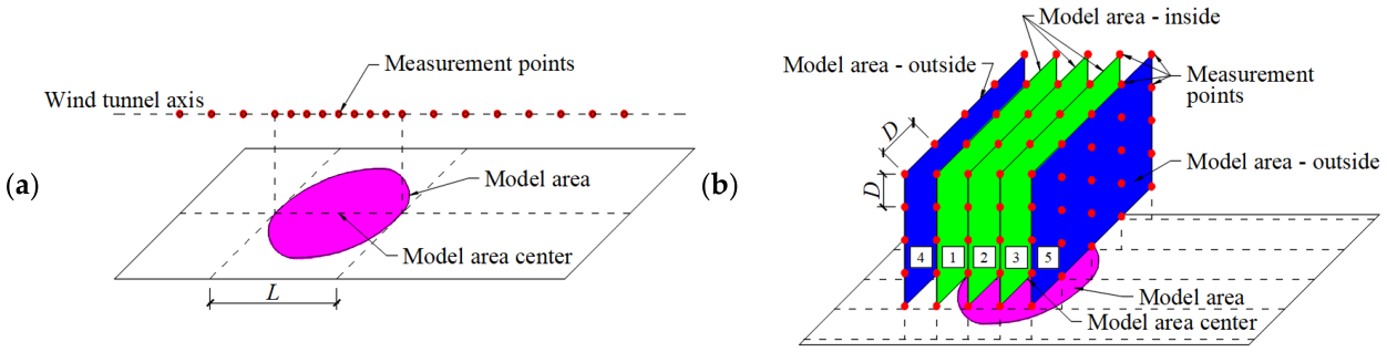
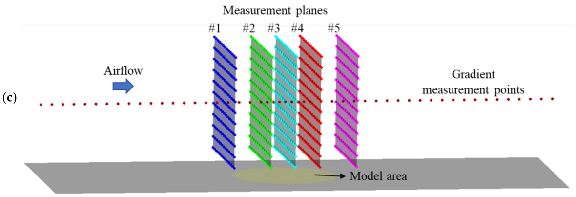
The standard specifies the measurement point configuration requirements for evaluating each metric. For the axial static pressure gradient, measurement points are distributed along the wind tunnel axis in the test section at intervals of less than 5% of the test section length. The test section of the Large Low-Speed Wind Tunnel is 21 m long, giving a maximum spacing of 1.05 m. A total of 51 points are therefore configured with adjacent spacings of 0.45 m outside the model area and 0.25 m inside the model area, as illustrated in Figure 3a. The model area is defined by the rotary turntable with an effective diameter of L = 4.25 m, which is adopted as the model area length in the subsequent calculations. For the turbulence intensity, dynamic pressure coefficient, and velocity direction deviation angles, the Chinese standard GJB 1179A-2012 requires at least five measurement planes, with at least three within the model area. The spacing between any two measurement points on each plane must not exceed $\sqrt{A}/15$, where A is the test section cross-sectional area. For the 8 m × 6 m test section (A = 48 m²), this gives a maximum spacing of 0.461 m. Five measurement planes are prescribed, denoted j = 1 to 5, with three located within the model area (j = 2, 3, 4) and one each located upstream (j = 1) and downstream (j = 5) of the model area, as illustrated in Figure 3b. Each measurement plane contains 143 measurement points spaced uniformly at 0.45 m, satisfying the spacing requirement.

The evaluation metrics are defined as follows.

(1) Axial static pressure gradient L × |dC_p/dx|. The static pressure at the measurement point i is denoted by p_i. Taking an arbitrary measurement point inside the test section as the reference static and dynamic pressures p_ref and q_ref, respectively, the static pressure coefficient at each measurement point i is:

$$C_{\mathrm{p},i}={\displaystyle \frac{(p_i-p_{\mathrm{ref}})}{q_{\mathrm{ref}}}}$$

(1)

The axial static pressure gradient is calculated by:

$$L\times \left|{\displaystyle \frac{d{C}_{\mathrm{p}}}{dx}}\right|=L\times \left|{\displaystyle \frac{n{\displaystyle {\displaystyle \sum _{i=1}^n}{x}_i{C}_{\mathrm{p}i}}-{\displaystyle {\displaystyle \sum _{i=1}^n}{C}_{\mathrm{p}i}}{\displaystyle {\displaystyle \sum _{i=1}^n}{x}_i}}{n{\displaystyle \sum _{i=1}^n{x_i}^2}-{\left({\displaystyle \sum _{i=1}^n{x}_i}\right)}^2}}\right|,$$

(2)

where x_i is the distance of point i to the test-section entrance, n is the total number of measurement points, and L = 4.25 m is the length of the model area.

(2) Turbulence intensity I. The turbulence intensity of point i in the measurement plane j is defined as:

$$I_{i,j}={\displaystyle \frac{u_{i,j}^{\prime }}{{\overline{U}}_{i,j}}},$$

(3)

where ${\overline{U}}_{i,j}$ is the mean velocity (m/s), $u_{i,j}^{\prime }$ is the root-mean-square (RMS) velocity (m/s). In the wind tunnel test, $u_{i,j}^{\prime }$ is obtained directly from velocity fluctuation measurements. Since the steady-state CFD simulation only solves the time-averaged quantities, $u_{i,j}^{\prime }$ cannot be obtained directly, and the RMS velocity is instead estimated using the turbulent kinetic energy k [36]:

$$u_{i,j}^{\prime }=\sqrt{{\displaystyle \frac{2}{3}}{k}_{i,j}}$$

(4)

The underlying approximation in Equation (4) assumes isotropic turbulence and introduces a degree of model dependence, since k is a modeled quantity whose magnitude depends on the turbulence closure. The isotropy assumption itself is discussed as a scope limitation in Section 3.3, and its implications of closure-dependence for the comparison between CFD and experimental turbulence intensity are discussed in Section 4.4.

(3) Dynamic pressure coefficient. The dynamic pressure coefficient quantifies the uniformity of the airflow velocity across a measurement plane. For measurement plane j:

$${\mu }_j={\displaystyle \frac{1}{m}}{\displaystyle {\sum }_{i=1}^m\left(\left|\frac{q_{i,j}}{{\overline{q}}_j}-1\right|\right)}, {\overline{q}}_j={\displaystyle \frac{1}{m}}{\displaystyle \sum _{i=1}^m{q}_{i,j}},$$

(5)

where $q_{i,j}$ is the dynamic pressure of the measurement point i (Pa), ${\overline{q}}_j$ is the mean value of the dynamic pressure of the measurement plane (Pa), and m is the total number of measurement points in the measurement plane (m = 143 points). The dynamic pressure coefficient is taken as the maximum across all measurement planes:

$$\mu =\underset{j}{\max }{\mu }_j$$

(6)

(4) Velocity direction deviation angles ∆α and ∆β. The velocity direction deviation angles quantify the misalignment of the local flow with respect to the wind tunnel axis. In the test section of the Large Low-Speed Wind Tunnel, the wind flows along the X direction, so the deviation angles at the measurement point i in the measurement plane j are

$$\left|\Delta {\alpha }_{i,j}\right|=\arctan \left({\displaystyle \frac{{\overline{U}}_{\mathrm{Y},i,j}}{{\overline{U}}_{\mathrm{X},i,j}}}\right), \left|\Delta {\beta }_{i,j}\right|=\arctan \left({\displaystyle \frac{{\overline{U}}_{\mathrm{Z},i,j}}{{\overline{U}}_{\mathrm{X},i,j}}}\right),$$

(7)

where ${\overline{U}}_{\mathrm{X},i,j}$, ${\overline{U}}_{\mathrm{Y},i,j}$, and ${\overline{U}}_{\mathrm{Z},i,j}$ are the mean wind velocity components in the X, Y, and Z directions (m/s). The deviation angles for each measurement plane are:

$$\Delta {\alpha }_j={\displaystyle \frac{1}{m}}{\displaystyle {\displaystyle \sum _{i=1}^m}\left|\Delta {\alpha }_{i,j}\right|}, \Delta {\beta }_j={\displaystyle \frac{1}{m}}{\displaystyle {\displaystyle \sum _{i=1}^m}\left|\Delta {\beta }_{i,j}\right|},$$

(8)

where m is the total number of measurement points in the measurement plane (m = 143 points). The velocity direction deviation angles are then taken as the maximum across all measurement planes:

$$\Delta \alpha =\underset{j=[1,5]}{\max }\Delta {\alpha }_j,\Delta \beta =\underset{j=[1,5]}{\max }\Delta {\beta }_j$$

(9)

The acceptance criteria specified by GJB 1179A-2012 for the low-speed wind tunnel are: L × |dC_p/dx| ≤ 0.005, I ≤ 0.10%, μ ≤ 0.20%, and Δα, Δβ ≤ 0.10°.

2.3. Wind Tunnel Test Data

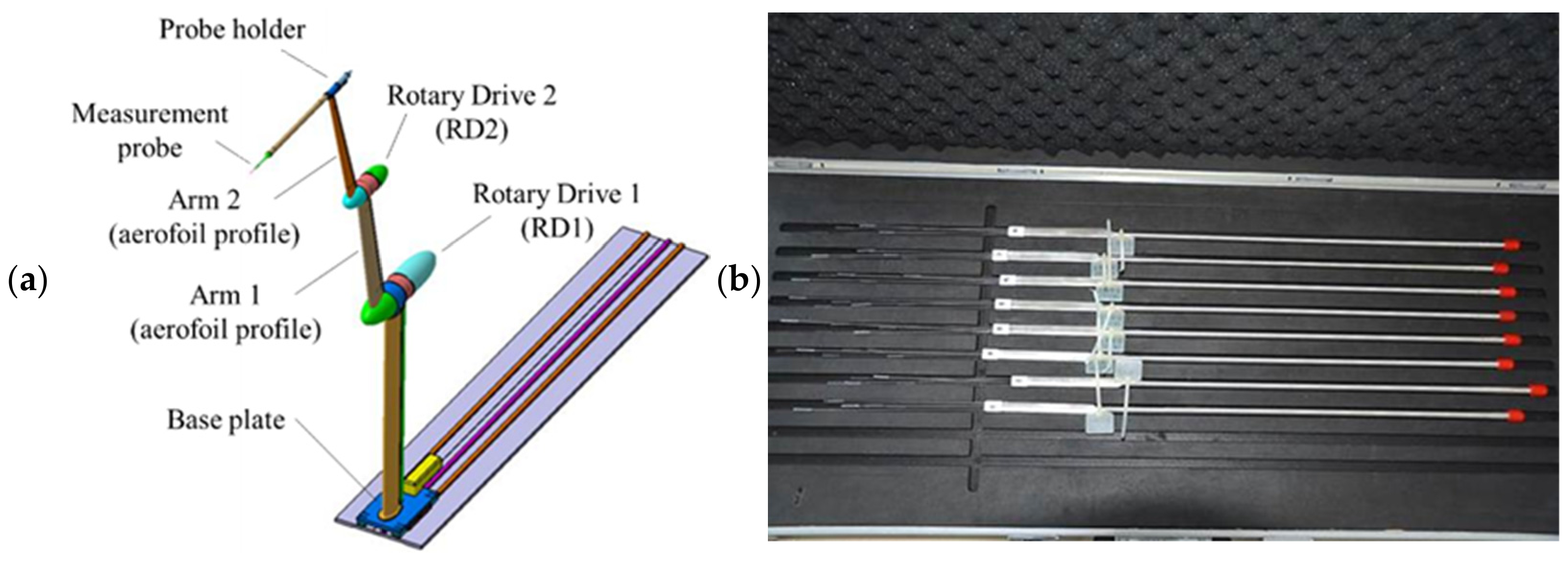
The wind tunnel test was conducted under the 130 m/s operating condition. Flow measurements were performed using a mobile rotary measurement frame system (ATE Aerotech, Heathfield, UK), which consists of a base plate, dual rotary drives, two rotating arms, and a probe holder accommodating probes up to 19 mm in diameter. The system was installed in the test section. The rotating arms are profiled to minimize local flow disturbances, and their motion is controlled by the built-in motion-control software (ATE Aerotech Pressure Probe Traverser control system), enabling automated traversal of the measurement planes defined in Section 2.2. Three probe types were employed: total pressure probes, five-hole probes, and wind velocity tubes. The total pressure probes and five-hole probes provide the static and dynamic pressure measurements used to evaluate the axial static pressure gradient and dynamic pressure coefficient. The five-hole probes also provide the three-component velocity measurements required for velocity direction deviation angles. The wind velocity tubes provide the velocity time histories from which the turbulence intensity is calculated. Details of the instrumentation systems are shown in Figure 4.

The static and dynamic pressure measurements were acquired using a PSI Optimus electronic pressure-scanning system, with an accuracy of 0.05% at full scale, sampled at 325 Hz for 1 min, as per the sampling duration requirement of GJB 1179A-2012. The turbulence-intensity measurement chain is built around a TSI constant-temperature hot-wire anemometry system (IFA300, 8 channels, sampling rate of 1000 Hz) with a maximum per-channel error below 0.3%. Probe positioning was provided by the rotary traverse mechanism described above, with a positional accuracy of ±0.12–0.37 mm and repeat positional accuracy of ±0.07–0.14 mm.

The wind tunnel test data are summarized in

Table 1. Wind tunnel test data of the Large Low-Speed Wind Tunnel.

Evaluation Metrics	Wind Tunnel Test	GJB 1179A-2012 [19]
Operating condition: Max. velocity	130.30 m/s	-
L × |dCp/dx|	0.0011	≤0.005
I	0.07%	≤0.10%
μ	0.15%	≤0.20%
Δα	0.09°	≤0.10°
Δβ	0.09°	≤0.10°

. The maximum velocity measured in the model area is 130.30 m/s, confirming the 130 m/s operating condition. The axial static pressure gradient is 0.0011, the maximum turbulence intensity is 0.07%, the dynamic pressure coefficient is 0.15%, and the velocity direction deviation angles are 0.09° in both axes. All metrics satisfy the acceptance criteria in GJB 1179A-2012. These data serve as the validation benchmark for the CFD simulations in Section 4.

3. Steady-State CFD Numerical Simulation Method

A large-scale low-speed wind tunnel is characterized by multiscale structures and complex geometric features, including corner sections, guiding vanes, contraction section, and flow-conditioning devices such as damping screens and honeycomb. This section presents the CFD simulation method, including the baseline computational model, the flow-conditioning devices representation modeling technique, and the common numerical settings.

3.1. CFD Numerical Simulation Method for Baseline Configuration

The geometric model of the Large Low-Speed Wind Tunnel was developed at 1:1 scale from the BIM model shown in Figure 5a, ensuring dimensional consistency with the wind tunnel’s internal aerodynamic surfaces. The guiding vanes with three-dimensional geometry in all corner sections were included. In the physical facility, the guiding vanes are connected horizontally to steel plates to improve structural stability during operation. These connecting plates were omitted in the geometric model due to their insignificant effect, as illustrated in Figure 5b. In the wind tunnel’s circuit, the flow passes through two corner sections, the diffusion section, the heat exchanger section, and the stable section, where the flow-conditioning devices are located before reaching the test section. These intervening components, particularly the corner sections’ guiding vanes and the flow-conditioning devices, are expected to dissipate fan-induced swirl and flow nonuniformities before the flow enters the contraction section. Therefore, the fan was not modeled and its effect on the flow is represented by the inlet boundary condition described below. Figure 5c shows the complete geometric model of the wind tunnel’s internal profiles.

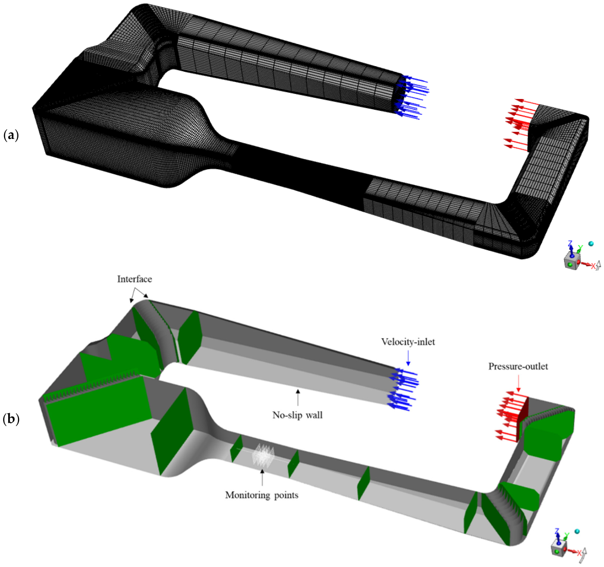
The computational mesh was generated in the software ICEM CFD using a combination of structured and unstructured meshes. Each section was discretized into a single domain using a structured mesh where the geometry permits, while an unstructured mesh was used for sections with more complex geometry. This mixed-discretization approach is consistent with the methodology used by Calautit et al. [28]. All section domains were connected via interface boundary conditions to form the full-scale wind tunnel model.

The numerical simulations were conducted using ANSYS FLUENT 22.0 in the steady-state solver. The airflow driven by the wind tunnel fan system was modeled using a velocity-inlet boundary condition on the upstream surface of the second diffusion section. The inlet velocity was determined from the continuity equation for incompressible flow:

$$\rho A_1{V}_1=\rho A_2{V}_2,$$

(10)

where ρ = 1.225 kg/m³ is the air density (assumed constant throughout the wind tunnel), and A₁, V₁, A₂, and V₂ are the cross-sectional area and wind speed at the upstream surface of the second diffuser section and test section, respectively, with V₂ = 130 m/s. This yields an inlet velocity of V₁ = 48.47 m/s. The inlet turbulence was specified using a turbulence intensity of 1% and a hydraulic diameter of 12.43 m. A pressure-outlet boundary condition was applied at the second corner surface with a gauge pressure of zero, representing ambient conditions. All surfaces were modeled as no-slip walls with standard wall functions. Monitoring points were prescribed within the test section, with the arrangement identical to the measurement points in the wind tunnel test. The developed full-scale computational model is shown in Figure 6.

The RNG k-ε turbulence model [37] was adopted for all configurations. The sensitivity of the results to the turbulence closure will be assessed in Section 4.4 by comparing with the SST k-ω turbulence model [38]. The transport equations of the turbulence models are given in the Appendix A. The SIMPLEC algorithm was employed for pressure–velocity coupling. The pressure term was discretised using the Standard scheme, the momentum term using the QUICK scheme, and the turbulent kinetic energy and dissipation rate using the second-order upwind scheme. Steady-state simulations were performed for 5000 iterations, with convergence confirmed by all residuals falling below 1 × 10⁻⁴ and the velocity and pressure at all monitoring points remaining constant.

Three grid densities were constructed for the grid sensitivity analysis: coarse, medium, and fine, with total element counts of 6,957,388, 10,073,503, and 12,301,110, respectively. The first cell height normal to the wall in the test section was set to 0.56 mm, 0.45 mm, and 0.38 mm for the coarse, medium, and fine grids, corresponding to Y+ values of 27.0~85.6, 20.5~67.8, and 17.8~62.3, respectively. Outside the test section, the first cell heights were 5.33, 4.00, and 2.85 mm for the coarse, medium, and fine grids. The grid growth rate was maintained below 1.2, and the minimum element quality (ICEM orthogonal quality criterion) was maintained above 0.3 for all grids. These Y+ values fall mostly within the log-law region (30 < Y+ < 300) in which standard wall functions are validated, with the lower end dipping into the buffer layer at isolated locations, consistent with the near-wall behavior expected for a complex, multiscale industrial geometry of this kind. All values remain above the Y+ ≈ 15 threshold below which standard wall function accuracy is known to deteriorate. Standard wall functions are the established, compliant near-wall treatment for a full-scale, high-Reynolds-number facility of this geometric complexity, applied here consistent with FLUENT’s near-wall treatment documentation [39]. They are adopted precisely because refining the grid to Y+ ≈ 1 across this entire multiscale 393 m circuit, a roughly 18- to 62-fold reduction in the fine grid’s own near-wall cell height, is not achievable within a practical computational budget, and would in any case require pairing that resolution with a low-Reynolds-number or wall-resolved near-wall treatment rather than the present formulation. Wall functions are formulated to reproduce the integrated wall shear stress and mean velocity profile of the log-law region itself [36], the same quantities that determine the bulk flow quality metrics targeted by the present evaluation, rather than the detailed near-wall gradient structure that only a fully resolved treatment can capture. Standard wall functions in this Y+ range are therefore sufficient for the present objectives [39].

3.2. Flow-Conditioning Device Modeling Method

In a full-scale CFD simulation of a large-scale low-speed wind tunnel, the flow-conditioning devices—one honeycomb layer and four layers of damping screens—cannot be modeled by explicit geometric resolution due to their complexity. Their geometric features are microscopic relative to the full-scale wind tunnel circuit, and resolving them would require prohibitively fine local mesh refinement. However, their effects on the flow cannot be neglected: previous studies have shown that damping screens and honeycomb significantly influence turbulence levels, velocity uniformity, and flow alignment in wind tunnel test sections [31,32,33,34,35]. A modeling strategy that captures their macroscopic influence without resolving their internal structure is therefore essential. The porous media framework [40], which has been applied to flow-conditioning devices in wind tunnel simulations [32,35], provides this capability. This section presents the porous media model as implemented in ANSYS FLUENT [39], the representation modeling of damping screens and honeycomb, and the parameter estimation method.

3.2.1. Porous Media Model

The pressure drop Δp across a porous medium is modeled by combining a viscous resistance term based on Darcy’s law with a nonlinear inertial resistance term introduced by Forchheimer [41]:

$$\Delta p=-\left({\displaystyle \frac{\eta }{a}}v\Delta m+C_2{\displaystyle \frac{1}{2}}\rho v^2\Delta m\right),$$

(11)

where η is the fluid dynamic viscosity (Pa·s), a is the face permeability (m²), v is the fluid velocity (m/s), ρ is the fluid density (kg/m³), C₂ is the pressure-jump coefficient (1/m), and Δm is the porous medium thickness (m). The viscous and inertial contributions are:

$$p_{\mathrm{viscous}}={\displaystyle \frac{\eta }{a}}v\Delta m,$$

(12)

$$p_{\mathrm{inertial}}=C_2{\displaystyle \frac{1}{2}}\rho v^2\Delta m$$

(13)

FLUENT provides two implementations of this framework. The porous jump model applies the pressure drop across a zero-thickness interface, defined by the face permeability a, the pressure-jump coefficient C₂, and the medium thickness Δm. The resistance acts isotropically on the flow. The porous zone model distributes the resistance over a finite-thickness fluid zone that is explicitly meshed in the computational domain. Because the resistance is applied volumetrically, the porous zone model permits anisotropic specification of the resistance coefficients in different coordinate directions.

3.2.2. Representation Modeling of Damping Screens and Honeycomb

The choice of representation for each device is governed by the relationship between the device thickness and the computational grid resolution. The damping screens have a physical thickness of 0.73 mm, which is smaller than the smallest computational cell in all three grid levels. Consequently, a finite-thickness porous zone cannot be constructed for these elements. Therefore, the damping screens were modeled as porous jumps, i.e., zero-thickness interfaces with an equivalent pressure drop. All four layers were modeled individually at their physical locations in the stable section, as specified in Section 2.1.

The honeycomb has a physical thickness of 800 mm, which is readily resolvable on the computational grid. Two candidate representations were therefore examined: a porous jump model, in which the honeycomb resistance is applied as a zero-thickness interface, and a porous zone model, in which the resistance is distributed over an 800 mm fluid zone explicitly meshed at the honeycomb location. For the porous zone model, the directional conditioning effect was represented by modifying the resistance coefficients in the transverse directions (Y and Z axes), which were amplified by a factor of 10⁶ relative to the streamwise direction (X axis), imposing a strong preferential flow alignment within the porous zone.

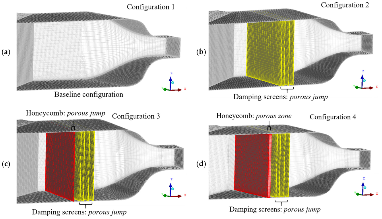
Four configurations were defined to isolate the individual and combined effects of the flow-conditioning devices:

• Configuration 1: Baseline—no flow-conditioning devices;
• Configuration 2: Damping screens only (four porous jump interfaces);
• Configuration 3: Damping screens + honeycomb modeled as porous jump;
• Configuration 4: Damping screens + honeycomb modeled as porous zone.

All configurations used the same computational grid, turbulence model, and boundary conditions. Differences in the predicted flow field between configurations can therefore be attributed to the representation of the flow-conditioning device. The configuration layouts are illustrated in Figure 7.

3.2.3. Parameter Estimation

As shown in Section 3.2.2, the porous media model requires three inputs: face permeability a, pressure-jump coefficient C2, and the porous medium thickness Δm. The thickness Δm is a known geometric quantity for each device. The face permeability a was estimated from the device porosity ϕ using the Kozeny–Carman formula [42,43]:

$$\varphi ={\left(1-d/l\right)}^2,$$

(14)

$$a={\displaystyle \frac{{\varphi }^3{d}^2}{150{\left(1-\varphi \right)}^2}},$$

(15)

where d is the separation layer thickness between openings and l is the opening diameter. The porosity and geometric parameters for each device were determined from the physical specifications given in Section 2.1.

The Kozeny–Carman formula was adopted for both devices because it relates permeability to porosity through a single characteristic opening length scale (Equation (15)), making it applicable to any perforated or cellular medium in which flow resistance is dominated by narrow passages, rather than being restricted to granular packed beds. A single, consistent permeability model was preferred for both devices for methodological uniformity, rather than mixing device-specific correlations. This choice is supported in the literature, where porosity-based permeability and loss-coefficient correlations of this type have been applied to perforated plates and wire screens [44,45,46], the same class of device as the honeycomb and damping screens modeled here.

The pressure-jump coefficient C₂ was estimated using the following procedure. For the 130 m/s operating condition, the mass flow rate is Q = ρ × V_test × A_test = 1.225 × 130 × 48 = 7644 kg/s. The area-weighted velocity at the stable section where the devices are located was determined from the continuity equation: V_stable = Q/(ρ × A_stable). The effective flow area through the porous medium was calculated as A_eff = ϕ × A_stable, giving an effective velocity V_eff = Q/(ρ × A_eff). The pressure drop across the device was then estimated from the velocity change:

$$\Delta p={\displaystyle \frac{1}{2}}\rho \left(V_{\mathrm{stable}}^2-V_{\mathrm{eff}}^2\right)$$

(16)

The viscous contribution p_viscous was calculated from Equation (12), and C₂ was obtained by rearranging Equation (13) using p_inertial = Δp − p_viscous. This procedure provides an engineering estimate of the porous media parameters based on the Bernoulli equation and the Kozeny–Carman permeability model. The estimated porous media parameters are summarized in

Table 2. Porous media model parameters of the flow-conditioning devices.

Flow-Conditioning Device	Thickness Δm	Porosity ϕ	Pressure Drop ∆p	Face Permeability a	pviscous	Pressure-Jump Coefficient C2	Pinertial
Honeycomb	800 mm	0.979	4.48 Pa	2.283 × 10−6 m2	81.53 Pa	−0.93 1/m	−77.05 Pa
Damping screen	0.73 mm	0.594	190.28 Pa	4.498 × 10−9 m2	37.75 Pa	2018.49 1/m	152.53 Pa

.

For the honeycomb, the estimated pressure-jump coefficient is C₂ = −0.93 m⁻¹. This arises because the Kozeny–Carman formula, originally developed for granular packed beds, estimates a face permeability that produces a viscous resistance term (p_viscous = 81.53 Pa) substantially larger than the total estimated pressure drop (Δp = 4.48 Pa) for this high-porosity (ϕ = 0.979) geometry. The negative C₂ functions as a correction coefficient that brings the total modeled pressure drop in line with the estimated physical value. This is numerically permissible in FLUENT, which accepts negative pressure-jump coefficients. The practical significance of this correction is small: the total honeycomb pressure drop (4.48 Pa) is more than an order of magnitude lower than the pressure drop across each damping screen layer (190.28 Pa), confirming that the honeycomb contributes a minor flow resistance relative to the damping screens. The primary role of the honeycomb in the CFD model is to condition directional flow through the anisotropic resistance of the porous zone, rather than to generate bulk pressure drop.

Equation (16) is mathematically negative in sign, since ϕ < 1 implies V_eff > V_stable, representing a pressure decrease in the flow direction, and this sign convention is preserved in the Δp column of Table 2. The subsequent decomposition into viscous and inertial contributions, p_inertial = Δp − p_viscous, and the resulting pressure-jump coefficients are, however, computed and reported using the positive-magnitude |Δp|, consistent with FLUENT’s porous zone input convention; Table 2 reports p_viscous, p_inertial, and C₂ on this positive-magnitude basis throughout.

In the FLUENT porous zone formulation, the inertial resistance coefficient C₂ is back-calculated as the residual required to match a target pressure drop once the viscous term is fixed (Equation (13)), rather than measured directly. FLUENT’s porous zone solver accepts negative values for this coefficient without restriction, and does so here. This is defensible on three grounds. First, the negative value is a direct consequence of the fitting procedure, not an ad hoc adjustment: the target pressure drop is fixed independently from the Bernoulli-based mass-flow accounting of Equation (16), the viscous term is fixed from the Kozeny–Carman permeability formula (Equation (15)), and C₂ is back-calculated as whatever residual reconciles the two. Because Kozeny–Carman, developed for granular packed beds, overestimates the viscous resistance of this honeycomb’s high-porosity (ϕ = 0.979), non-granular geometry, exceeding the Equation (16) target, the residual comes out negative. This is a property of the decomposition, not of the honeycomb’s physical behavior: a passive device cannot add energy to the flow, so the combined viscous-plus-inertial resistance, the only quantity with direct physical meaning, remains valid regardless of the sign of either individual term.

Second, the magnitude of this combined resistance is independently verified. An independent, Kozeny–Carman-free honeycomb pressure-loss correlation [47] gives K_h = λ_h·(L_h/D_h+3)·(1/ϕ)² + (1/ϕ−1)², with λ_h = 0.375·RN^−0.1(Δ/D_h)^0.4 for RN ≤ 275 and λ_h = 0.214 (Δ/D_h)^0.4 for RN > 275—a correlation that, like passive-resistance correlations in general, is non-negative by construction (even for an idealized smooth wall, Δ→0, K_h reduces to (1/ϕ−1)² ≥ 0). Using the honeycomb’s own geometry (L_h = 800 mm, ϕ = 0.979, D_h ≈ 38 mm) and the facility’s stable-section flow conditions (V_eff ≈ 13.0 m/s), sweeping across wall surface roughness from an idealized smooth surface to the typical stainless steel sheet range (Δ = 0–6.3 μm), this correlation predicts a total Δp of 0.05–26.3 Pa. The magnitude obtained from the Bernoulli/Kozeny–Carman procedure above (4.48 Pa) falls within this independently derived pressure loss, toward its smooth end, and the honeycomb’s contribution remains more than an order of magnitude below that of the damping screens’ (190.28 Pa).

Third, FLUENT’s porous zone formulation applies the combined resistance, the sum of the viscous and inertial terms in Equation (11), as a single momentum source at each cell, rather than applying the two terms separately. The solver therefore acts on this combined value, whose magnitude is independently verified above, and not on the sign of either constituent term in isolation. The negative C₂ accordingly carries no separate numerical or physical consequence for the honeycomb’s modeled function.

3.3. Scope of the Present Methodology

The present evaluation adopts a steady-state RANS formulation. Thus, unsteady phenomena such as fan-induced periodic disturbances or transient flow separation are not characterized here. Furthermore, turbulence intensity is estimated from the modeled turbulent kinetic energy k via Equation (4), which assumes isotropic velocity fluctuations, the classical approach for extracting turbulence intensity from a steady RANS solution. The wind tunnel measurement instead obtains RMS velocity directly from the fluctuating velocity probe signal, without invoking isotropy. Near-wall and contraction-accelerated flows are not generally isotropic, so the CFD-predicted turbulence intensity should be read as internally consistent within the RANS framework rather than as a bias-free measure of the absolute turbulence level reported by the wind tunnel test.

The damping screens and honeycomb are represented through calibrated porous media source terms rather than through resolved geometry. This is not merely a computational convenience: the damping screens have a physical thickness of 0.73 mm, smaller than the smallest computational cell at any grid level used in this study (Section 3.2.2), so explicit resolution is not a computationally available alternative at this facility scale. More fundamentally, the flow quality objectives evaluated here, velocity uniformity, and mean pressure gradient over the full test-section cross-section, depend on each device’s aggregate effect on the macroscopic flow field, not on the detailed flow structure through individual screen wires or honeycomb cells, which is exactly the effect a calibrated porous media source term is designed to reproduce.

This study evaluates flow quality at a single operating condition, 130 m/s (Ma ≈ 0.38), the compressibility effect of which was explicitly assessed in Section 4.5. Since compressibility effects diminish as Mach number decreases, this represents the most demanding condition addressed within the present framework; speeds above 130 m/s fall outside its validated scope. The porous media representation and parameter estimation method developed in Section 3.2, damping screen and honeycomb resistance coefficients anchored to a Bernoulli-based pressure-drop estimate and cross-verified against an independent correlation, is not specific to this facility and can be adopted for other large-scale, closed-circuit wind tunnels, provided the resistance parameters are re-estimated from each facility’s own geometry and porosity using the same procedure. The specific parameter values reported in Table 2 are additionally tied to the 130 m/s operating condition at which they were estimated under the incompressible Bernoulli formulation of Section 3.2.3. Since V_stable and V_eff depend on operating speed, a change in operating wind speed requires the resistance parameters to be re-estimated for the new condition rather than be reused directly.

4. Results and Discussion

4.1. Baseline Configuration: Grid Sensitivity, Capability, and Limitations

Table 3. Comparisons of baseline CFD results on coarse, medium, and fine grids with wind tunnel test data and acceptance criteria.

Evaluation Metrics	Coarse	Medium	Fine	Wind Tunnel Test	GJB 1179A-2012
Max. velocity	132.05 m/s	132.13 m/s	132.03 m/s	130.30 m/s	-
L × |dCp/dx|	0.0031	0.0032	0.0032	0.0011	≤0.005
I	0.89%	1.61%	1.72%	0.07%	≤0.1%
μ	0.21%	0.28%	0.32%	0.15%	≤0.20%
Δα	0.41°	0.40°	0.39°	0.09°	≤0.10°
Δβ	0.26°	0.26°	0.27°	0.09°

compares the CFD results of the baseline configuration (Configuration 1 in Figure 7) on coarse, medium, and fine grids with the wind tunnel test data and the acceptance criteria in GJB 1179A-2012. The baseline configuration uses the explicit tunnel geometry without flow-conditioning devices.

The grid sensitivity falls into two distinct groups. The maximum velocity, axial static pressure gradient, and velocity direction deviation angles Δα and Δβ are largely insensitive to grid refinement, with variations across the three grids remaining within 0.10 m/s, 0.0001, 0.02°, and 0.01°, respectively. In contrast, the turbulence intensity I and dynamic pressure coefficient μ show greater sensitivity, particularly between the coarse and medium grids. However, in both cases, the rate of change diminishes markedly from medium to fine: I and μ change by only 0.11 and 0.04 percentage points between the medium and fine grids, compared with 0.72 and 0.07 percentage points between the coarse and medium grids, indicating that the solution is approaching grid independence. This monotonic, diminishing-increment trend, together with a pass/fail conclusion against the GJB 1179A-2012 acceptance criterion that is stable across the medium and fine grids, constitutes robust, directly relevant convergence evidence for a facility of this geometric complexity. Therefore, the medium grid is selected as the working grid density for all subsequent configurations, as it provides a reasonable balance between computational cost and solution accuracy: the remaining grid sensitivity from medium to fine is small, while the fine grid requires higher computational cost.

Furthermore, the sensitivity of the results to the inlet turbulence intensity was investigated by increasing the turbulence intensity prescribed on the inlet to 10% on the baseline configuration. The predicted test-section turbulence intensity changed from 1.61% to 1.62% (an increase of 0.01 percentage points), with the other four evaluation metrics essentially unchanged or marginally improved (maximum velocity 132.13 → 131.97 m/s; axial static pressure gradient 0.00324 → 0.00329; dynamic pressure coefficient 0.28% → 0.23%; Δα 0.40° → 0.34°; Δβ 0.26° → 0.24°). An inlet turbulence intensity of 1% is therefore a faithful and sufficiently conservative assumption for a facility of this scale and configuration, and the reported results are demonstrated to be insensitive to this boundary condition over a full order-of-magnitude change in the assumed inlet value.

Using the selected medium grid, the baseline configuration was compared against the wind tunnel test data and the acceptance criteria. The predicted maximum velocity on the medium grid (132.13 m/s) is within 1.5% of the wind tunnel test data (130.3 m/s). The axial static pressure gradient satisfies the acceptance criterion, indicating that the streamwise pressure development is adequately captured by the explicit tunnel geometry alone. However, the other evaluation metrics, such as I, μ, Δα, and Δβ, are all substantially overpredicted and exceed the acceptance limits. The largest discrepancy occurs in I, which exceeds the wind tunnel test data by more than an order of magnitude.

These results define the capabilities and limitations of the baseline explicit-geometry model. The axial static pressure gradient, which characterizes the streamwise pressure development along the test section, is adequately reproduced by the explicit tunnel geometry alone. This is physically consistent: the pressure gradient is governed primarily by the test-section geometry and the contraction ratio, both of which are modeled explicitly. In contrast, the turbulence intensity, velocity uniformity, and flow alignment are not controlled solely by the tunnel geometry. These metrics depend on the conditioning of the incoming flow by the upstream damping screens and honeycomb, which are absent from the baseline configuration. The overpredictions should therefore be attributed to the omission of flow-conditioning devices rather than to grid inadequacy. Further refinement from the medium to the fine grid produces only limited changes in these metrics, while the discrepancies with the experimental values remain large.

Although the axial static pressure gradient satisfies the acceptance criterion, the predicted value on the medium grid (0.0032) exceeds the experimental data (0.0011) by a factor of approximately three. This ratio should be interpreted in the context of the physical scale of the underlying quantity. The wind tunnel test data indicate that the static pressure variation along the test section is minimal, with absolute C_p changes of order 10⁻³. Resolving such small pressure variations to high precision is inherently challenging in a full-scale CFD simulation, where the finite cell size imposes a resolution floor that cannot be reduced without a disproportionate increase in computational cost. At this scale, a small absolute deviation in the predicted axial static pressure gradient—the difference between 0.0032 and 0.0011 is 0.0021—translates into a large ratio while remaining physically insignificant in terms of the absolute error. Both values satisfy the acceptance criterion by comfortable margins (limit of 0.005), confirming that the test section exhibits a nearly uniform streamwise pressure distribution in both the simulation and the experiment. The overprediction does not affect the remaining four evaluation metrics, whose discrepancies with the experimental values are attributable to the omission of flow-conditioning devices as discussed in the following subsections.

4.2. Influence of Damping Screens on Flow Quality

Configuration 2 (see Figure 7b) introduces the four layers of damping screens, modeled as porous jumps using the parameters derived in Section 3.2.

Table 4. Comparisons of evaluation metrics among CFD simulations with/without flow-conditioning devices, GJB 1179A-2012, and wind tunnel test.

Evaluation Metrics	Configuration 1 (Medium Grids)	Configuration 2: Damping Screens	GJB 1179A-2012	Wind Tunnel Test
Max. velocity	132.13 m/s	131.82 m/s	-	130.30 m/s
L × |dCp/dx|	0.0032	0.0033	≤0.005	0.0011
I	1.61%	0.03%	≤0.1%	0.07%
μ	0.28%	0.08%	≤0.20%	0.15%
Δα	0.40°	0.10°	≤0.10°	0.09°
Δβ	0.26°	0.07°		0.09°

compares the CFD results of Configuration 2 with the baseline configuration, the wind tunnel test data, and the acceptance criteria.

The inclusion of damping screens transforms the predictive performance of the CFD simulation. For the baseline configuration, only the axial static pressure gradient meets the acceptance criterion, whereas for Configuration 2, all evaluated metrics are within the acceptance limits. The improvement is concentrated entirely in the four metrics that the baseline failed to reproduce—I, μ, ∆α and ∆β—while the maximum velocity and axial static pressure gradient remain essentially unchanged (132.13 m/s vs. 131.82 m/s and 0.0032 vs. 0.0033, respectively). The overprediction of the axial static pressure gradient relative to the experimental value noted in Section 4.1 persists at a similar magnitude, confirming that this discrepancy is unrelated to the flow conditioning representation. This asymmetry is physically significant: it indicates that the damping screens locally modify the flow quality delivered to the test section without altering the circuit-level mean-flow structure that governs the streamwise pressure development. However, the comparison with the wind tunnel test data shows that the inclusion of damping screens brings all metrics substantially closer to the measured flow quality. The turbulence intensity, which exceeds the wind tunnel test data by more than an order of magnitude for the baseline configuration, is now predicted to be within the same order of magnitude (0.03% vs. 0.07%). The dynamic pressure coefficient decreases from 0.28% to 0.08%, substantially closer to the wind tunnel test data of 0.15%. The velocity direction deviation angles show the closest agreement: Δα = 0.10° and Δβ = 0.07° against wind tunnel test data of 0.09° in both axes.

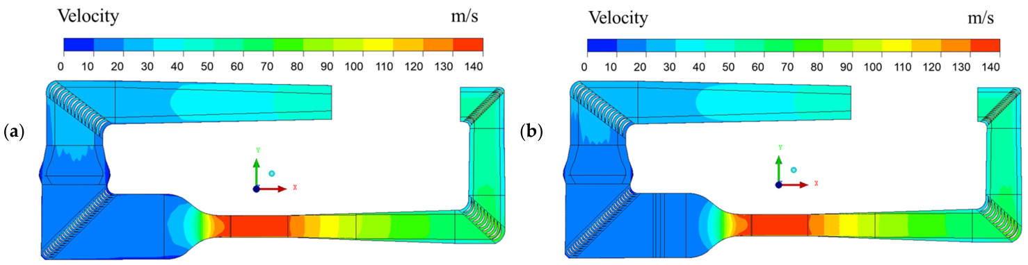
The circuit-level mean velocity contours in Figure 8 confirm the above interpretation. The large-scale flow pattern through the tunnel remains broadly similar between Configurations 1 and 2, with the primary velocity features—acceleration through the contraction, deceleration in the diffusers, turning in the corner sections—preserved in both cases. The differences are localized to the stable section and the contraction entrance, where Configuration 2 exhibits a more symmetric velocity distribution and smoother streamwise gradients. This is consistent with the physical role of the damping screens: they attenuate upstream nonuniformities and transverse disturbances, delivering a better-conditioned inflow to the contraction. The contraction section preserves and reinforces this improvement: a more uniform incoming profile yields a correspondingly more uniform accelerated profile at the test-section entrance.

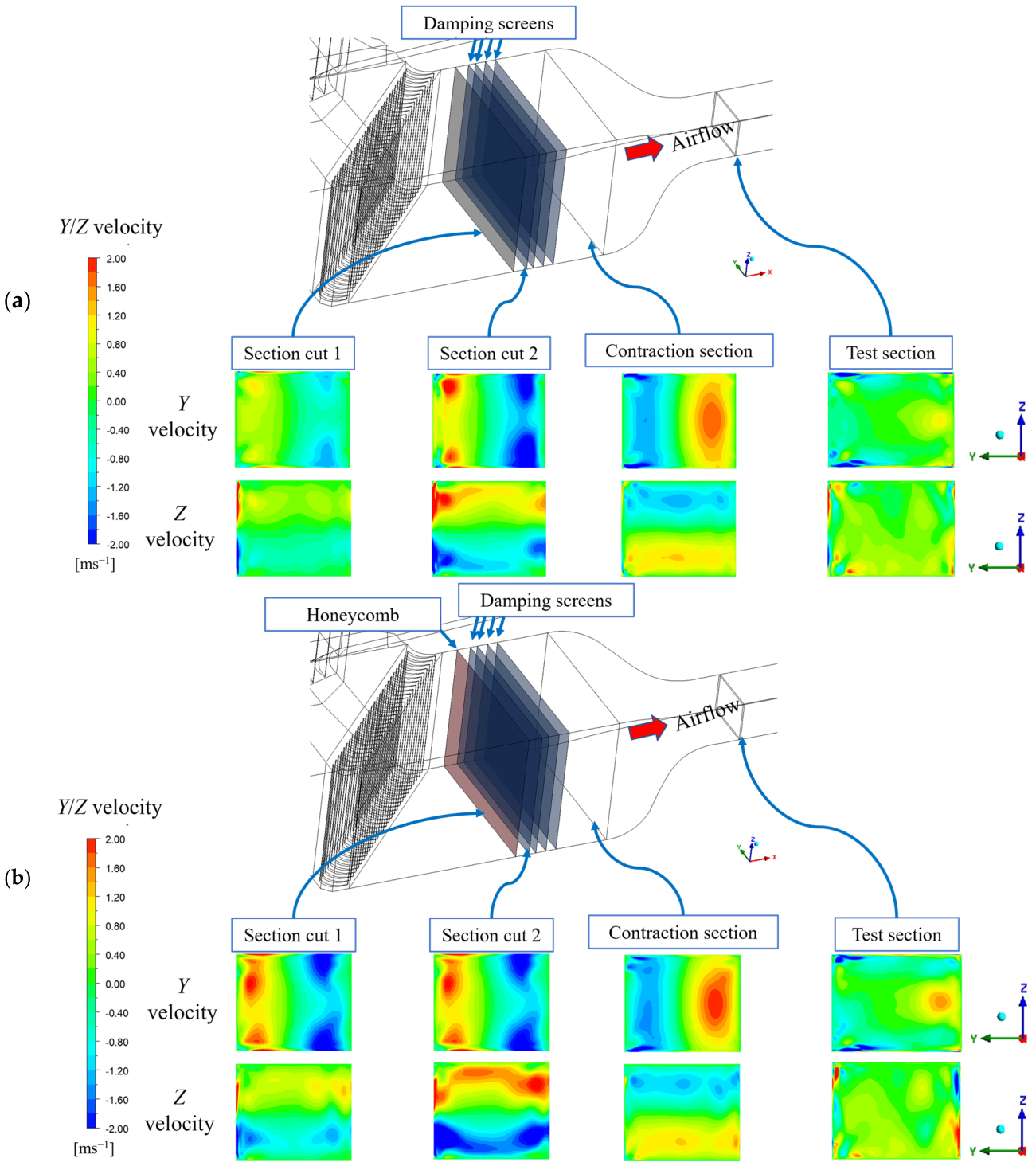
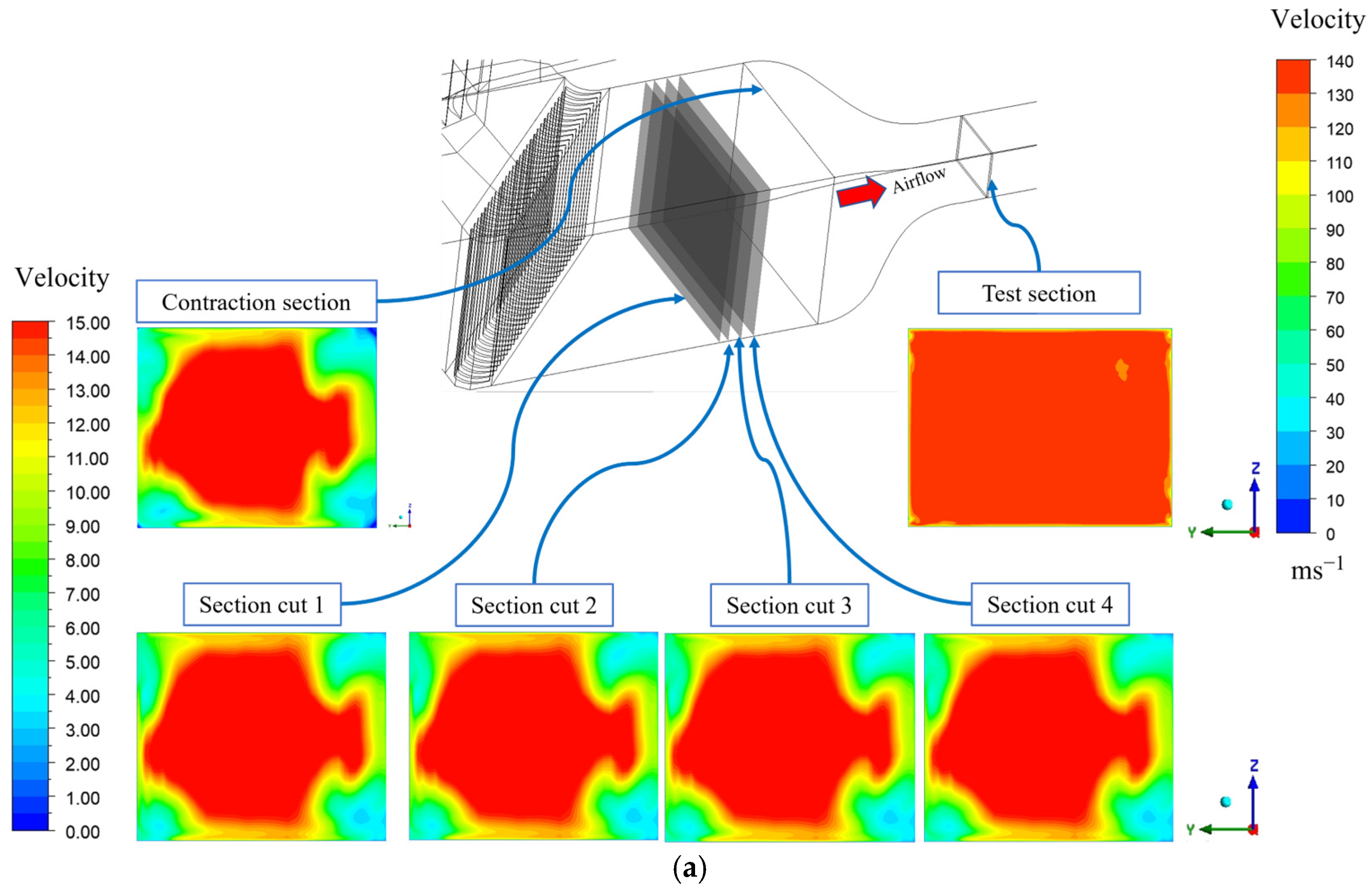
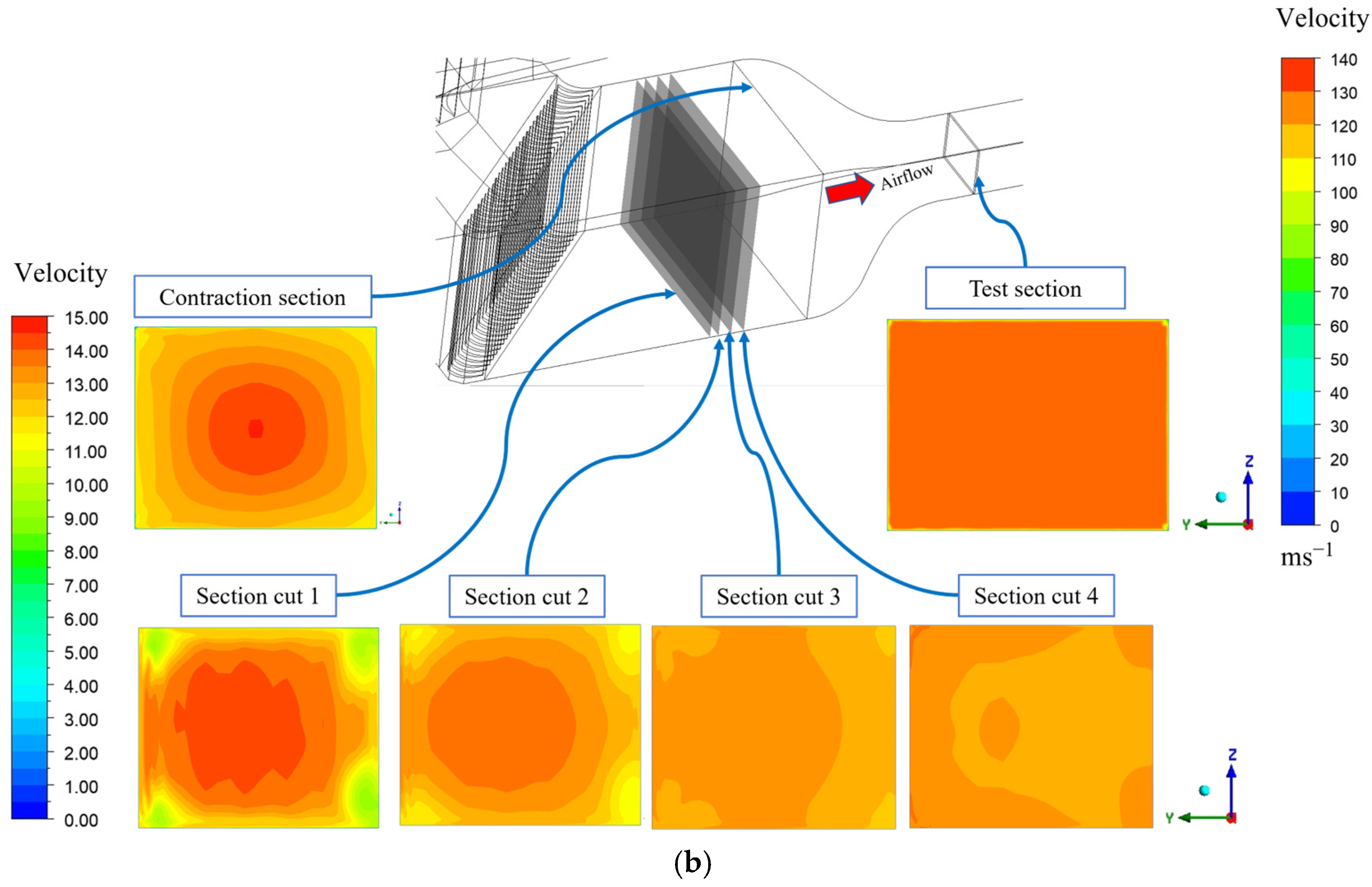
The cross-sectional mean wind velocity contours at successive section planes in Figure 9 make the conditioning mechanism explicit. In Configuration 1, the four section cuts show essentially the same non-uniform distribution at every plane: without screens, no conditioning mechanism acts on the flow between those locations, and the spatial pattern of elevated core velocity and reduced wall-adjacent velocity is preserved through the stable section. In Configuration 2, the same four section cut planes (located at the damping screen location) reveal a monotonically improving distribution from cut 1 to cut 4, with each successive plane showing a more spatially uniform profile than the one preceding it.

This progressive improvement is a direct consequence of the inertial resistance term in the Forchheimer term formulation (see Equation (13)). Because the resistance scales with the square of the local velocity magnitude, the pressure penalty is disproportionately large in regions of higher velocity and proportionally reduced in regions of lower velocity. This velocity-dependent resistance constitutes a self-equalizing mechanism: each screen reduces the flow most strongly where it is fastest and least strongly where it is slowest, reducing the cross-sectional velocity gradient at each successive damping screen. The diminishing incremental improvement from cut 1→2 to cut 2→3 to cut 3→4 is consistent with this mechanism: each successive screen acts on an already more uniform profile, so the velocity gradient that drives the equalizing effect is progressively exhausted. By the fourth screen, the velocity distribution is substantially more uniform than that near the stable section entrance, with residual spatial variation confined largely to the wall-adjacent boundary layer.

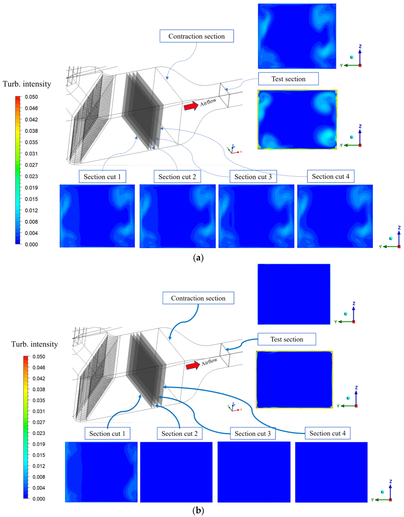
The turbulence-intensity contours in Figure 10 reveal a qualitatively different conditioning pattern. Rather than a progressive reduction observed in the velocity field (see Figure 9b), the turbulence intensity collapses substantially at the first screen plane and shows negligible further reduction at the downstream planes. This behavior reflects the indirect mechanism by which the porous jump model modifies the turbulence field. The porous jump boundary condition acts exclusively on the momentum equations through the pressure-drop source term. It does not directly modify the turbulent kinetic energy k or dissipation rate ε. Therefore, the turbulence reduction emerges not from direct action on k, but from the change each screen induces in the velocity field. The non-uniform flow arriving at the first screen plane sustains elevated turbulence intensity through continuous shear production: the large spatial velocity gradients in the incoming flow generate turbulent kinetic energy through the production term $G_k=-\rho \overline{u_i^{\prime }{u}_j^{\prime }}{\displaystyle \frac{\mathsf{\partial }{u}_j}{\mathsf{\partial }{x}_i}}$. The first damping screen eliminates the dominant source of this production by promoting a more uniform velocity distribution and reduces the transverse velocity components, which eliminates the velocity gradients responsible for shear production. Without this production source, k decays by dissipation toward the background level, bringing turbulence intensity to a significantly reduced level. The shear production mechanism that sustained the elevated incoming turbulence is effectively eliminated after the first screen. Subsequent screens impose their inertial resistance on an already low-gradient, low-turbulence flow field, and produce correspondingly little further modification of k. The near-plateau in turbulence intensity from the second screen plane onward is therefore not indicative of ineffective conditioning by the downstream screens, but of a saturation condition in which the primary production mechanism has already been eliminated.

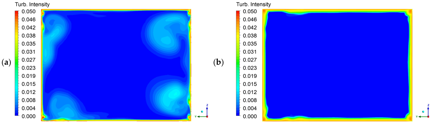
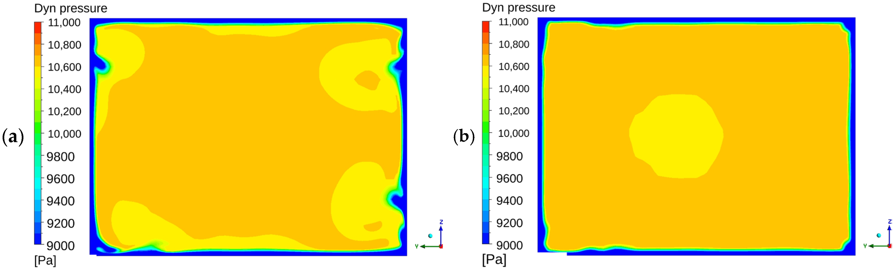
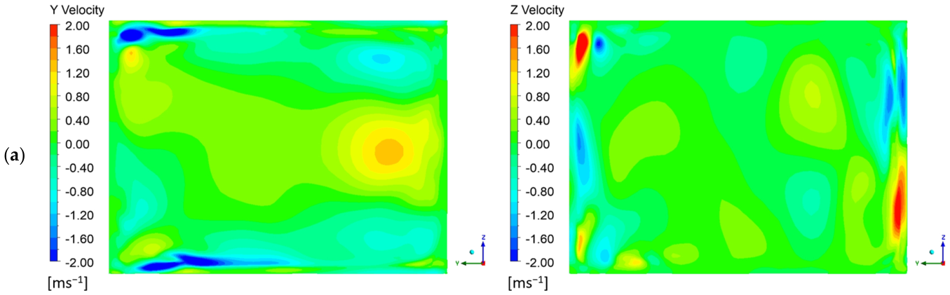
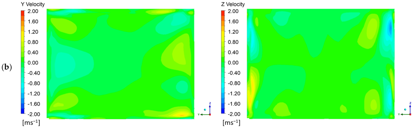
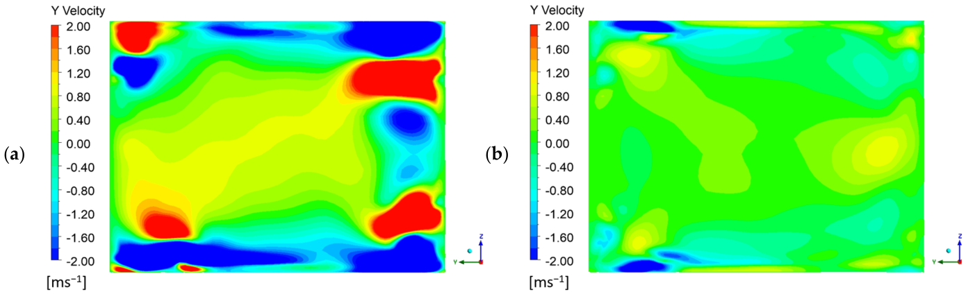
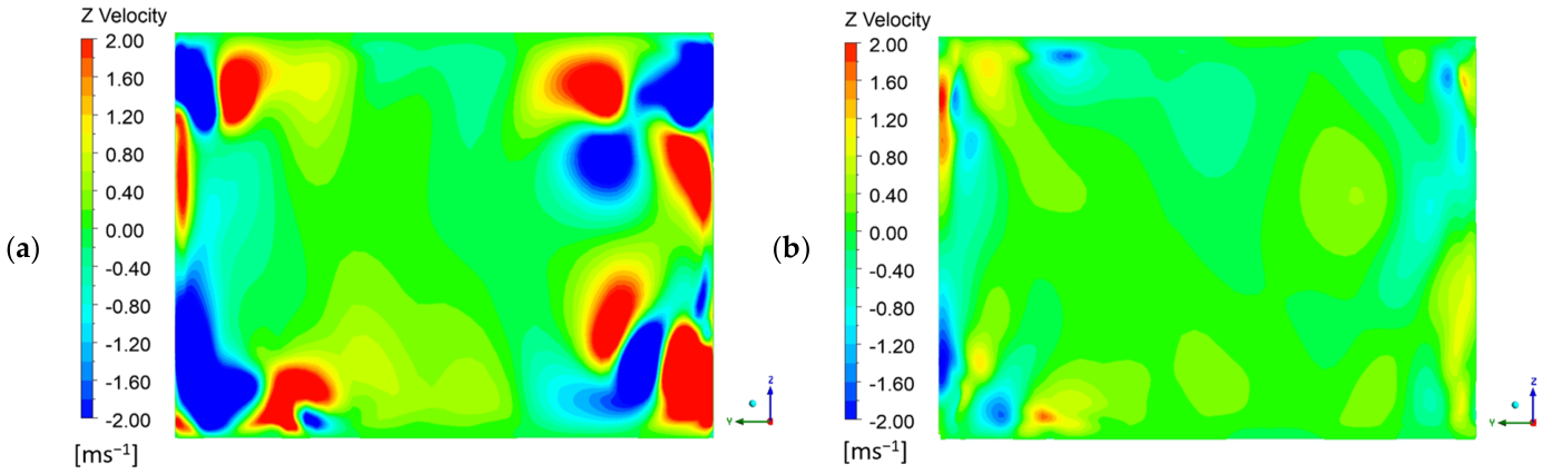
The test-section contours reveal how this improved upstream conditioning propagates into the flow quality metrics. The turbulence intensity contours at the model area center inside the test section (Figure 11) show the most pronounced change: For the baseline configuration, elevated turbulence extends from the corners deep into the interior of the test section, whereas in Configuration 2, the core region is dominated by uniformly low values, with residual turbulence confined to a thin wall-adjacent perimeter. The dynamic pressure contours (Figure 12) show a corresponding improvement in spatial uniformity—the asymmetric high-dynamic pressure region present in the baseline configuration is replaced by a nearly uniform distribution across the measurement plane, consistent with the reduction in μ from 0.28% to 0.08%. The transverse velocity components (Figure 13 and Figure 14) are effectively suppressed throughout the core region, with residual nonzero components confined to the near-wall zone and leaving low-velocity pockets in the core region. This explains the sharp improvements in Δα (from 0.40° to 0.10°) and Δβ (from 0.26° to 0.07°).

A consistent flow characteristic emerges from these observations. The damping screens act on the incoming flow upstream of the contraction, attenuating turbulence and increasing velocity spatial uniformity. A more uniform spatial distribution inherently reduces transverse velocity gradients, further suppressing directional deviations. The residual imperfections in Configuration 2—the thin perimeter of elevated turbulence, the minor near-wall transverse velocities—are wall-bounded effects that the damping screens, located far upstream, cannot be expected to eliminate. The important conclusion is that damping screen representation is not a secondary refinement but a necessary component of a physically credible CFD model of this facility: without it, the model fails the acceptance criteria; with it, all criteria are satisfied. On this basis, the following subsection examines the additional effect of the honeycomb and compares the two candidate modeling representations using porous jump and porous zone introduced in Section 3.2.2.

4.3. Influence of Honeycomb Representation on Flow Quality

Table 5. Comparisons of evaluation metrics among CFD simulations with different flow-conditioning devices, GJB 1179A-2012, and wind tunnel test.

Evaluation Metrics	Configuration 2: Damping Screens	Configuration 3: Damping Screens + Porous Jump Honeycomb	Configuration 4: Damping Screens + Porous Zone Honeycomb	GJB 1179A-2012	Wind Tunnel Test
Max. velocity	131.82 m/s	131.84 m/s	131.84 m/s	-	130.30 m/s
L × |dCp/dx|	0.0033	0.0027	0.0033	≤0.005	0.0011
I	0.03%	0.02%	0.02%	≤0.1%	0.07%
μ	0.08%	0.10%	0.08%	≤0.20%	0.15%
Δα	0.10°	0.13°	0.04°	≤0.10°	0.09°
Δβ	0.07°	0.08°	0.03°		0.09°

compares the damping screens-only configuration (Configuration 2) with the two damping screens-plus-honeycomb configurations, in which the honeycomb is represented as either a porous jump (Configuration 3) or a porous zone (Configuration 4).

The addition of the honeycomb produces only a modest further reduction in turbulence intensity, from 0.03% to 0.02% in both representations. The maximum velocity is unaffected. The axial static pressure gradient remains at 0.0033 in the porous zone representation (Configuration 4), identical to the damping screens-only case, consistent with the expectation that the honeycomb’s primary function is directional conditioning rather than modification of the streamwise pressure development. The porous jump representation (Configuration 3) yields a notably lower value of 0.0027, a departure for which there is no physical basis, as the honeycomb is not expected to reduce the axial static pressure gradient. This suggests that the zero-thickness pressure discontinuity imposed by the porous jump interface introduces an unphysical perturbation to the streamwise pressure field, providing further evidence that this representation does not faithfully reproduce the macroscopic effect of the honeycomb. In both cases, the overprediction of the axial static pressure gradient relative to the experimental value noted in Section 4.1 persists, and both values remain within the acceptance criterion.

The more revealing comparison lies in the metrics associated with the honeycomb’s primary physical function—attenuation of transverse velocity components and flow straightening. Here, the two representations diverge sharply, and this discrepancy determines the preferred modeling choice. The porous zone model (Configuration 4) reduces Δα from 0.10° to 0.04° and Δβ from 0.07° to 0.03°, while preserving μ at 0.08%. The porous jump model (Configuration 3) produces the opposite effect: Δα increases from 0.10° to 0.13°, exceeding the acceptance limit of 0.10°, and μ increases from 0.08% to 0.10%. This is a critical distinction. The porous jump representation not only fails to reproduce the flow-straightening effect of the honeycomb but also actively degrades the alignment and uniformity metrics that Configuration 2 had already brought within the acceptance limits.

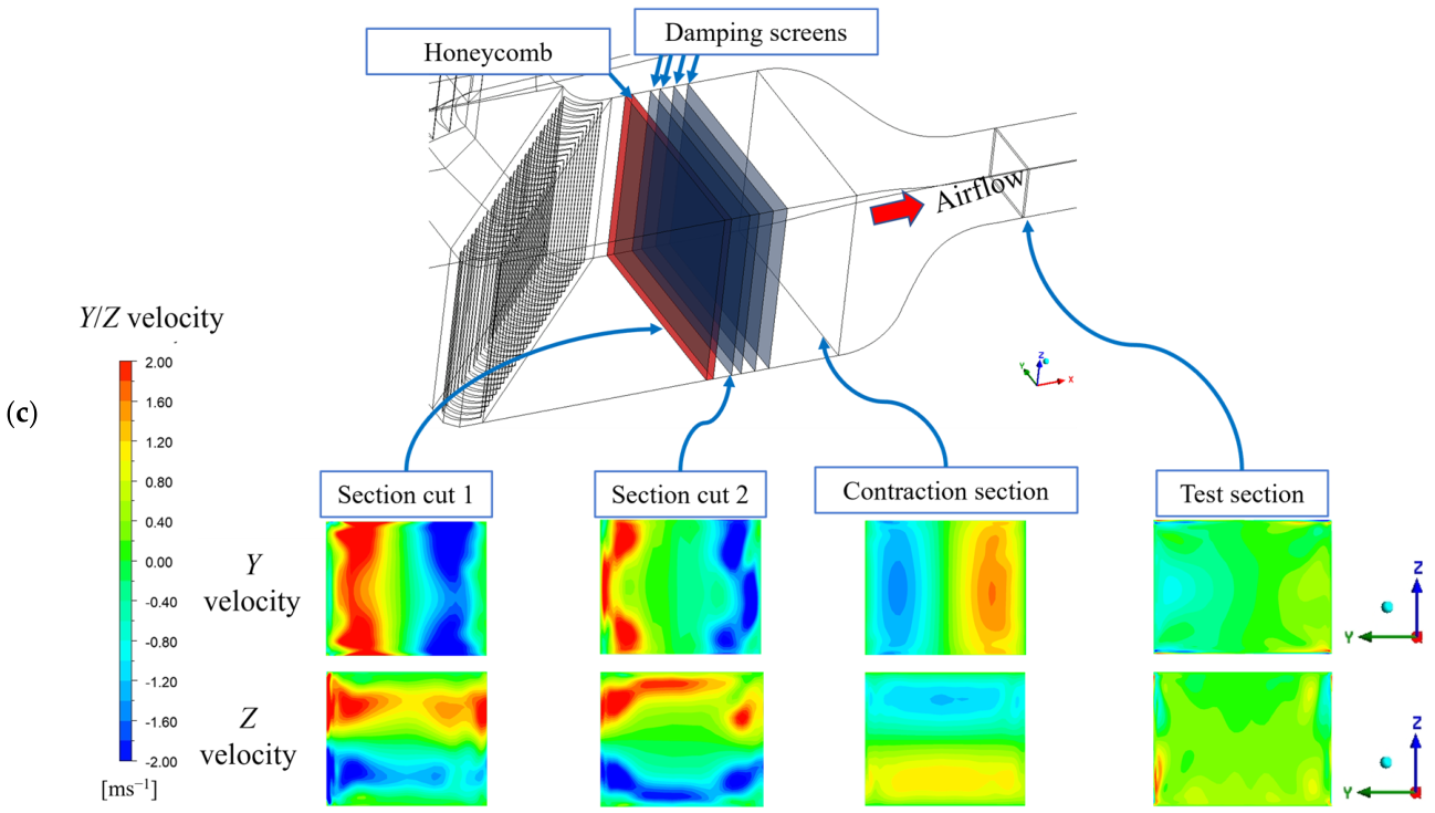
The transverse velocity contours at successive upstream section planes in Figure 15 reveal the contrasting conditioning behavior of the two honeycomb representations relative to the damping screens-only reference case of Configuration 2, and provide direct visual evidence for the mechanism underlying the metric divergence observed in Figure 16 and Table 5.

In Configuration 2, the transverse velocity components are progressively suppressed through the self-equalizing inertial resistance mechanism established in Section 4.2. The porous jump parameters of the damping screens, derived from a high-solidity wire-mesh geometry, yield a large inertial resistance coefficient C₂, sufficient to produce a measurable preferential suppression of transverse velocity components at each successive interface. The result is a monotonically improving transverse velocity distribution delivered to the contraction entrance.

Configuration 3 departs from this pattern. The porous jump parameters of the honeycomb reflect the high porosity of the physical device and yield a substantially smaller C₂ than the damping screens. When applied isotropically at a zero-thickness interface, this mild resistance produces a uniform scalar pressure drop across all velocity components without preferential attenuation of the transverse directions. The zero-thickness formulation provides no spatial extent for directional conditioning to develop. Consequently, the section planes downstream of the honeycomb in Configuration 3 show transverse velocity levels marginally worse than Configuration 2: the isotropic porous jump contributes no flow straightening, while the abrupt pressure discontinuity perturbs the local flow field without a physical basis. The degradation of Δα from 0.10° to 0.13°, which exceeds the acceptance limit, is the consequence of the absence of distributed directional conditioning.

Configuration 4 exhibits a qualitatively distinct three-stage conditioning progression that warrants detailed examination. At the honeycomb entrance plane, the transverse velocity distribution exhibits an organized, approximately symmetric pattern with higher magnitudes than that in Configuration 2. This elevation does not reflect active transverse suppression at this location. Rather, the entrance plane captures the flow at the face of the porous zone before the distributed anisotropic resistance has acted over any meaningful spatial depth. The elevated transverse magnitude relative to Configuration 2 is attributable to the high transverse resistance of the porous zone formulation, introducing a localized pressure perturbation at the entrance face as a consequence of the zone’s strong directional resistance against transverse momentum acting on the incoming flow field, before redistribution has had spatial extent to develop. However, the approximately symmetric contour at this plane is mechanistically significant: it indicates that the anisotropic resistance results in a spatially uniform distribution across the cross-section, in contrast to the localized, less symmetric perturbation introduced by the isotropic porous jump of Configuration 3. By damping screen 1—after the flow has traversed the full 800 mm physical depth of the porous zone—the distributed directional conditioning has acted over the entire thickness of the device, progressively redirecting transverse momentum toward the axial direction, thereby reproducing the flow-straightening mechanism of the physical honeycomb. The transverse velocity distribution at this plane is the best among all three configurations, with elevated magnitudes confined to the wall-adjacent region and the core region effectively straightened. In the third stage, this well-conditioned, axially aligned profile enters the contraction section, where the combined effect of honeycomb straightening and four successive damping screens is amplified by the contraction-induced acceleration and then propagates directly into the test section. The evaluation metrics, Δα = 0.04° and Δβ = 0.03°, are the quantitative outcome of this cumulative flow-conditioning mechanism.

The strong directional constraint imposed by the anisotropic porous zone formulation produces velocity direction deviation angles, Δα = 0.04° and Δβ = 0.03°, which are significantly lower than the corresponding wind tunnel test values of 0.09° in both axes. This underprediction is expected because the honeycomb is modeled as an idealized anisotropic resistance within a geometrically idealized computational domain. In the physical facility, residual flow disturbances originate from sources that are absent or simplified in the current CFD simulation, such as surface roughness on aerodynamic surfaces, structural members within the tunnel cross-section, inter-section pressure gaps, accumulated construction tolerances over a 393 m circuit, and the wind tunnel fan. Each of these sources introduces minor but meaningful perturbations to the velocity direction field that the simulation cannot replicate. Therefore, the CFD simulation captures the full directional conditioning potential of the honeycomb without the influence of these physical imperfections and simplifications, resulting in alignment metrics that serve as a lower bound on what the physical facility can achieve under ideal conditions, rather than directly reproducing the measured values.

The transverse flow progression in Configuration 4 and its absence in Configuration 3 establish the physical basis for the preference of the porous zone representation on grounds that extend beyond metric compliance alone: the porous zone reproduces the spatial mechanism of the physical device, whereas the porous jump, irrespective of its parameter values, is structurally incapable of representing a process that is distributed over finite depth. Configuration 4 is accordingly adopted as the selected configuration for the turbulence model sensitivity analysis in Section 4.4 and the compressibility assessment in Section 4.5.

The transverse resistance factor introduced in Section 3.2.2 (10⁶ amplification factor relative to the streamwise direction) was not tuned to an experimental target. It was set large enough that the transverse resistance term dominates the momentum balance in those directions, approximating the physical limit of a honeycomb cell wall being impermeable to transverse flow. The sensitivity of the results to this factor was tested on Configuration 4 by sweeping it across four orders of magnitude: 10⁴, 10⁶ (the adopted value), and 10⁸.

Table 6. Sensitivity of evaluation metrics to the transverse resistance factor of the honeycomb porous zone, Configuration 4.

Evaluation Metrics	Transverse Resistance Factor 104	Transverse Resistance Factor 106 (Adopted)	Transverse Resistance Factor 108	GJB 1179A-2012	Wind Tunnel Test
Max. velocity	131.84 m/s	131.84 m/s	131.83 m/s	-	130.30 m/s
L × |dCp/dx|	0.0032	0.0033	0.0032	≤0.005	0.0011
I	0.02%	0.02%	0.02%	≤0.1%	0.07%
μ	0.08%	0.08%	0.08%	≤0.20%	0.15%
Δα	0.04°	0.04°	0.04°	≤0.10°	0.09°
Δβ	0.03°	0.03°	0.03°		0.09°

compares the resulting evaluation metrics. All five metrics are essentially unchanged across this range. This flat response over four orders of magnitude confirms the resistance term dominates the momentum balance at the lower end and shows the specific value chosen is not a significant source of solution uncertainty.

4.4. Influence of Turbulence Model on Flow Quality

Table 7. Comparisons of evaluation metrics among CFD simulations with different turbulence models, GJB 1179A-2012, and wind tunnel test.

Evaluation Metrics	Configuration 4: RNG k-ε	Configuration 4: SST k-ω	GJB 1179A-2012	Wind Tunnel Test
Max. velocity	131.84 m/s	131.89 m/s	-	130.30 m/s
L × |dCp/dx|	0.0033	0.0033	≤0.005	0.0011
I	0.02%	0.36%	≤0.1%	0.07%
μ	0.08%	0.08%	≤0.20%	0.15%
Δα	0.04°	0.05°	≤0.10°	0.09°
Δβ	0.03°	0.04°		0.09°

compares the flow quality predictions obtained from the RNG k-ε and SST k-ω turbulence models for Configuration 4. The purpose of this comparison is to assess whether the principal conclusions of the present study, regarding the roles of the damping screens and the honeycomb representation, remain stable when the turbulence closure is changed. The transport equations and model constants for the two turbulence closures are presented in Appendix A.

The two closure models produce nearly identical results for four of the five evaluated metrics, and all of these values remain well within the acceptance limits for both models. The axial static pressure gradient is 0.0033 under both closures, the dynamic pressure coefficient remains at 0.08%, and the velocity direction deviation angles vary by only 0.01° in both axes. The overprediction of the axial static pressure gradient, discussed in Section 4.1, persists at a similar magnitude and remains within the acceptance criterion. Furthermore, the maximum velocity difference is less than 0.1 m/s. This indicates that the global flow structure is insensitive to turbulence modeling, and once the flow-conditioning devices are included in the model, the predicted velocity uniformity and flow alignment are governed primarily by flow conditioning, which therefore holds independently of the turbulence model.

The turbulence intensity is the sole exception. The RNG k-ε model predicts I = 0.02%, whereas the SST k-ω model predicts I = 0.36%—a difference of more than an order of magnitude. This difference is consequential: the RNG k-ε prediction satisfies the acceptance limit of 0.10%, whereas the SST k-ω prediction exceeds it. The wind tunnel test data (0.07%) lies between the two predictions. This sensitivity was anticipated in Section 2.2, where the turbulence intensity was identified as a model-dependent quantity estimated from the turbulent kinetic energy k via Equation (4). The value of k is among the most model-dependent outputs of a steady RANS simulation.

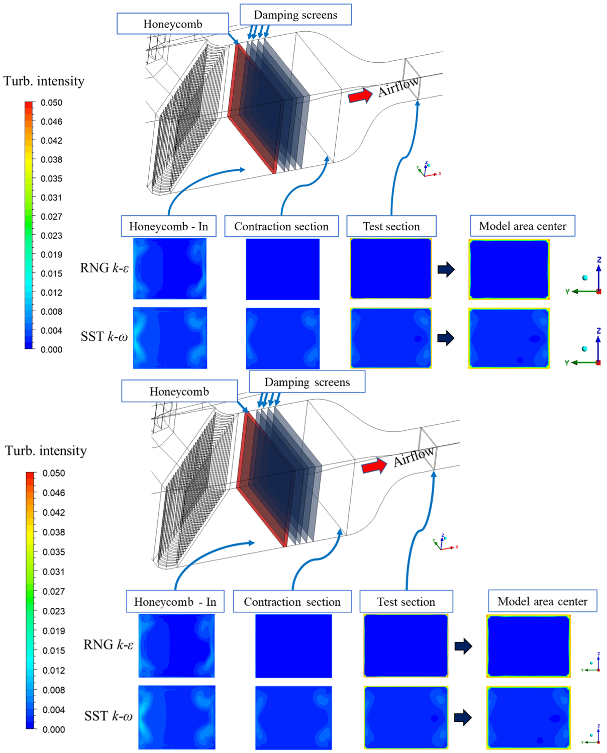
The turbulence intensity contours progression in Figure 17 provides direct spatial evidence for the mechanistic origin of this divergence. At the honeycomb entrance plane, both turbulence models produce broadly similar distributions, confirming that the two models condition the upstream flow field equivalently and that the metric discrepancy observed in Table 7 does not originate within the stable section. The divergence emerges progressively downstream. At the contraction section plane, the SST k-ω model already exhibits locally high turbulence intensity in the wall-adjacent and corner regions, whereas the RNG k-ε model produces a spatially uniform, low-turbulence intensity distribution across the full cross-section. This divergence amplifies through the test section and is fully resolved at the model area center plane: under RNG k-ε turbulence closure, elevated turbulence intensity is confined to a thin perimeter strip adjacent to the tunnel walls, with the section’s core dominated by uniformly low values; under SST k-ω turbulence closure, substantially thicker regions of elevated turbulence intensity extend inward from all four walls and corner junctions into the interior of the evaluation zone, encroaching on the measurement region.

The spatial origin of this divergence, the wall and corner region under SST k-ω, is physically consistent with the structural difference between the two closures. The SST k-ω formulation employs a k-ω model in the near-wall region specifically designed to preserve turbulent kinetic energy within boundary layers under adverse pressure gradients and flow separation conditions. However, the present application is characterized by a well-developed, attached boundary layer along the smooth contraction walls under a favorable pressure gradient. This formulation sustains a higher k in the wall-adjacent region than the RNG k-ε model predicts under the same flow condition. The higher k generated at the walls and corners propagates inward as the flow accelerates through the contraction, producing the thick elevated turbulence intensity regions observed at the model area center. The RNG k-ε model, through its strain-rate-dependent correction term in the ε transport equation, produces enhanced dissipation under the rapid straining conditions imposed by the contraction. This mechanism preferentially diminishes k as the flow accelerates, yielding a low, spatially uniform turbulence intensity distribution at the model area center with residual elevation confined to the thin wall-adjacent strip where boundary layer production remains locally active. Therefore, the contraction section acts as a discriminating amplifier: both models arrive at its entrance with similar turbulence intensity distributions, but the contraction’s strain field interacts differently with each model’s dissipation mechanism, producing categorically different outcomes at the test section.

A second, independent physical consideration supports the same conclusion. The CFD geometry is an idealized, as-designed representation with smooth walls and no manufacturing or installation imperfections, whereas the wind tunnel test necessarily reflects the as-built facility, including joint gaps, surface roughness, and screen/honeycomb installation tolerances. A lower turbulence intensity in the idealized model relative to the physical facility is therefore the physically expected direction of discrepancy: the RNG k-ε prediction (I = 0.02%) sits below the wind tunnel test value (0.07%) in exactly this expected direction and by a plausible margin, whereas the SST k-ω prediction (I = 0.36%) substantially overpredicts the test value, in the opposite direction from what the idealization gap would predict. Both physical arguments converge on the same conclusion. The RNG k-ε prediction (I = 0.02%) deviates from the wind tunnel test value (I = 0.07%) by only 0.05 percentage points, consistent with the idealized-wall gap discussed above. The SST k-ω prediction (I = 0.36%) deviates by 0.29 percentage points, nearly six times larger, in the opposite direction, which that gap cannot explain and instead reflects the mechanism discussed above. This closer, physically grounded agreement with the experimental benchmark, not merely the acceptance-criterion outcome (RNG k-ε satisfies the GJB 1179A-2012 limit of I ≤ 0.10% while SST k-ω does not), is the primary basis for retaining the RNG k-ε closure adopted in Section 3.1 as the appropriate turbulence model for this facility and operating condition. All four other evaluated metrics are essentially insensitive to the turbulence closure once the flow-conditioning devices are present, so this sensitivity is confined to turbulence intensity alone.

4.5. Effect of Compressibility at 130 m/s Operating Condition on Flow Quality

The preceding simulations adopt incompressible formulations with constant air density ρ = 1.225 kg/m³. As for the 130 m/s operating wind speed in the test section, the local Mach number reaches approximately Ma ≈ 0.38, which exceeds the conventional threshold beyond which compressibility effects may no longer be negligible (Ma > 0.3). This subsection assesses whether the air incompressible assumption materially affects the predicted flow quality metrics by comparing incompressible and compressible simulations of the same full-scale model.

The compressible simulation uses Configuration 4 with the RNG k-ε turbulence model, on the same computational grid, boundary conditions, and identical porous media parameters as the incompressible case. The only modifications are: the air density is governed by the ideal-gas law rather than kept constant, with the energy equation model activated, and the density term is discretized using the second-order upwind scheme. All other numerical settings remain the same as those described in Section 3. In particular, the inlet velocity boundary condition (V₁ = 48.47 m/s) is held identical to the incompressible case rather than re-calibrated to reproduce the 130 m/s test-section target under the compressible formulation. Mass is conserved throughout by the governing continuity equation regardless of the density treatment, since the model is a closed, steady-state circuit with no leakage paths, but the mass flow rate itself is free to differ between the two formulations because it depends on the local inlet density, fixed at ρ = 1.225 kg/m³ in the incompressible case and solved from the ideal-gas law in the compressible case. Re-calibrating the inlet velocity to force the compressible case back to the 130 m/s target would confound the compressibility effect with a deliberate change in mass flow rate, leaving it unclear which of the two was responsible for any resulting difference. The resulting increase in maximum velocity to 143.65 m/s, discussed below, is therefore the expected, deliberate consequence of holding the inlet velocity condition fixed to isolate the compressibility effect, not a discrepancy against the 130 m/s target.

Table 8. Comparisons of evaluation metrics among the incompressible and compressible CFD simulations, GJB 1179A-2012, and wind tunnel test.

Evaluation Metrics	Configuration 4: Incompressible	Configuration 4: Compressible	GJB 1179A-2012	Wind Tunnel Test
Max. velocity	131.84 m/s	143.65 m/s	-	130.30 m/s
L × |dCp/dx|	0.0033	0.0048	≤0.005	0.0011
I	0.02%	0.02%	≤0.1%	0.07%
μ	0.08%	0.06%	≤0.20%	0.15%
Δα	0.04°	0.06°	≤0.10°	0.09°
Δβ	0.03°	0.04°		0.09°

compares the flow quality evaluation metrics obtained from the incompressible and compressible formulations. The metrics that depend on the flow-conditioning device—turbulence intensity, dynamic pressure coefficient, and velocity direction deviation angles—are effectively invariant between formulations. The turbulence intensity remains at 0.02% under both formulations, the dynamic pressure coefficient decreases marginally from 0.08% to 0.06%, and the velocity direction deviation angles differ by at most 0.02° in Δα and 0.01° in Δβ. All four metrics remain within the GJB 1179A-2012 acceptance criteria under both formulations.

The global quantities of maximum velocity and axial static pressure gradient respond differently. The maximum velocity increases from 131.84 m/s to 143.65 m/s and the axial static pressure gradient increases from 0.0033 to 0.0048 between the two formulations. The compressible pressure gradient value of 0.0048 approaches but remains within the acceptance criterion of L × |dC_p/dx| ≤ 0.005. These increases reflect the physical mechanism of compressibility: as the flow accelerates through the contraction, local air density decreases, and continuity demands a higher velocity at the test section inlet than the incompressible formulation predicts due to the isentropic relationship that couples density and velocity. Accordingly, the axial static pressure gradient becomes steeper through density–velocity coupling.

A multi-quantity thermodynamic verification is conducted in this study to prove the consistency of the compressible simulation with classical isentropic flow theory [48], whose thermodynamic factors can be expressed by the following equations.

$${\displaystyle \frac{{\rho }_{\mathrm{local}}}{{\rho }_0}}={\left(1+{\displaystyle \frac{\gamma -1}{2}}{\mathrm{Ma}}^2\right)}^{-{\displaystyle \frac{1}{\gamma -1}}},$$

(17)

$${\displaystyle \frac{T_{\mathrm{local}}}{T_0}}={\left(1+{\displaystyle \frac{\gamma -1}{2}}{\mathrm{Ma}}^2\right)}^{-1}$$

(18)

For an ideal gas with the ratio of specific heats of γ = 1.4, the isentropic relations at Ma = 0.38 yield a density ratio ρ_local/ρ₀ ≈ 0.931, and a temperature ratio T_local/T₀ ≈ 0.972. Taking the stagnation air density and temperature as ρ₀ = 1.225 kg/m³ and T₀ = 300 K, respectively, the theoretical test section local density is ρ_local ≈ 1.141 kg/m³, and the theoretical local temperature is T_local ≈ 291.5 K. Then, the theoretical test section velocity V_test can be derived from continuity and the estimated ρ_local, resulting in V_test ≈ 139.64 m/s. The CFD predictions of the air density and temperature are approximately 1.103 kg/m³ and 290.9 K, respectively, which are consistent with these theoretical values within the margins, which can be attributed to non-isentropic losses accumulated through the full 393 m tunnel circuit, including viscous dissipation through corner sections, guiding vanes, and flow-conditioning devices, which are absent from the idealized isentropic relation. Correspondingly, the CFD Max. velocity of 143.65 m/s overestimates the theoretical local velocity of 139.64 m/s by less than 2.9% due to reduced air density. Therefore, the above multi-quantity agreement between CFD and isentropic theory confirms that the compressible simulation reproduces the thermodynamic state of the test section in a physically consistent manner.

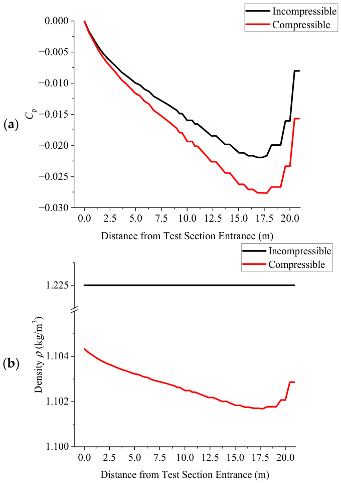
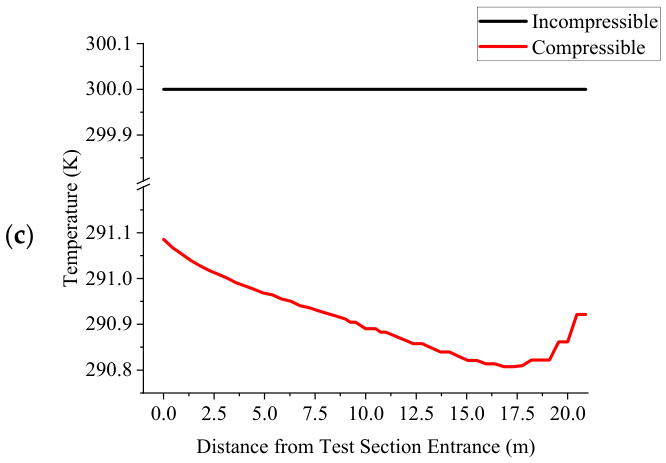
The centerline distributions of C_p, air density, and temperature in Figure 18 confirm this behavior directly. In Figure 18a, both curves originate at zero at the test-section entrance, where the reference static pressure pref is defined, and the compressible curve lies consistently below the incompressible curve, with the separation widening progressively along the test section. This is reflected in Table 8. L × |dCp/dx| rises from 0.0033 to 0.0048, consuming 96% of the ≤ 0.005 acceptance margin, compared with 66% under the incompressible formulation. Figure 18b,c show the corresponding density and temperature distributions. The centerline density in the compressible case decreases by less than 0.25% over the 21 m test section length, and the centerline temperature by approximately 0.10%, both consistent with the isentropic relations at Ma = 0.38, while both remain constant by formulation in the incompressible case. The remaining four metrics, detailed above, are governed by the upstream flow-conditioning devices established in Section 4.2 and Section 4.3. Only the axial static pressure gradient, the one metric shown in Section 4.1 to be governed by tunnel geometry rather than the conditioning devices, responds to compressibility through this density–velocity coupling. This confirms the incompressible formulation as a sufficient and credible evaluation basis for Section 4.1, Section 4.2, Section 4.3 and Section 4.4.

5. Conclusions

The findings of this study provide a practical full-scale steady-state CFD methodology for evaluating the flow quality of a large-scale, operational low-speed wind tunnel, validated against measured wind tunnel test data and establishing a hierarchy of which modeling choices materially affect predicted flow quality and which do not, offering practical reference for the CFD-based evaluation, design, or retrofit of comparable large-scale low-speed wind tunnel facilities. The main conclusions in this study are summarized as follows.

• The baseline configuration, constructed from the explicit tunnel geometry, reproduces the axial static pressure gradient at test section within the acceptance criterion but substantially overpredicts turbulence intensity, dynamic pressure coefficient, and velocity direction deviation angles. Therefore, explicit geometry alone is insufficient to reproduce the measured flow quality.
• The inclusion of damping screens, modeled as porous jumps, provides the dominant correction in the CFD framework. All evaluated metrics are brought within the acceptance limits and substantially closer to the wind tunnel test data. This correction is physically attributable to the velocity-dependent inertial resistance in the Forchheimer formulation, which constitutes a self-equalizing mechanism: each screen reduces the flow most strongly where it is fastest, progressively reducing cross-sectional velocity gradients and collapsing the shear production term responsible for the elevated turbulence. Accordingly, damping screen representation is not an optional refinement, but a prerequisite for physical credibility in a CFD model of this facility at the operating condition evaluated in this study.
• The additional inclusion of the honeycomb produces only a modest further change in the scalar flow quality metrics. However, the two candidate representations yield markedly different predictions for the alignment-related metrics. The porous zone model preserves or improves all metrics and remains fully compliant with the acceptance criteria, whereas the porous jump model degrades the velocity direction deviations and dynamic pressure coefficient, with Δα exceeding the acceptance limit. Therefore, the porous zone representation is preferred for the honeycomb representation based on both results-driven and physical grounds.
• The axial static pressure gradient, dynamic pressure coefficient, and velocity direction deviations are insensitive to the choice between the RNG k-ε and SST k-ω models, confirming that these metrics are governed primarily by the tunnel geometry and flow-conditioning devices included. The turbulence intensity is the sole closure-sensitive metric, with the RNG k-ε model providing a closer prediction to the wind tunnel test result. Accordingly, the RNG k-ε model is the more suitable turbulence closure for the present application.
• The effect of compressibility at the 130 m/s operating condition (Ma ≈ 0.38) was investigated by comparing incompressible and compressible formulations of the full-scale model. Only the axial static pressure gradient responds materially, increasing from 0.0033 to 0.0048 while remaining compliant with the ≤0.005 criterion. The remaining flow conditioning-dependent metrics, namely the turbulence intensity, dynamic pressure coefficient, and the two velocity direction deviation angles, remain effectively invariant and within their acceptance limits under both formulations. Therefore, the incompressible formulation is confirmed as a sufficient and credible basis for the evaluation at the current Mach number.

The close agreement between the calibrated CFD predictions and the measured wind tunnel test data across all evaluated configurations indicates that the steady-state formulation and the porous media representation of the damping screens and honeycomb do not materially compromise the reported flow quality conclusions, despite neither resolving unsteady flow phenomena nor the conditioning devices’ internal geometry.

Collectively, the modeling workflow, explicit tunnel geometry, porous media calibration, and staged comparisons offer a transferable CFD procedure for designing or retrofitting large-scale, low-speed wind tunnels. The workflow itself is adaptable to the specific parameters of the facility and operating conditions. Reproducing test-section flow without costly physical trials, this method is adaptable to future facilities and conditions, supporting resource-efficient and sustainable development of large-scale wind tunnel test infrastructure.

References

1. Cermak, J.E. Applications of wind tunnels to investigation of wind-engineering problems. AIAA J. 1979, 17, 679–690. [Google Scholar] [CrossRef] [Scilit] [PubMed]
2. Cermak, J.E. Wind-tunnel development and trends in applications to civil engineering. J. Wind Eng. Ind. Aerodyn. 2003, 91, 355–370. [Google Scholar] [CrossRef] [Scilit]
3. Chanetz, B. A century of wind tunnels since Eiffel. Comptes Rendus Mécanique 2017, 345, 581–594. [Google Scholar] [CrossRef] [Scilit]
4. Kramer, C.; Gerhardt, H.J.; Regenscheit, B. Wind tunnels for industrial aerodynamics. J. Wind Eng. Ind. Aerodyn. 1984, 16, 225–264. [Google Scholar] [CrossRef] [Scilit]
5. Mehta, R.D.; Bradshaw, P. Design rules for small low-speed wind tunnels. Aeronaut. J. 1979, 83, 443–453. [Google Scholar] [CrossRef] [Scilit]
6. Huang, M.; Wang, Z.W. A review of wind tunnel-based virtual flight testing techniques for evaluation of flight control systems. Int. J. Aerosp. Eng. 2015, 2015, 672423. [Google Scholar] [CrossRef] [Scilit]
7. Tang, D.; Dowell, E.H. Experimental aeroelastic models design and wind tunnel testing for correlation with new theory. Aerospace 2016, 3, 12. [Google Scholar] [CrossRef] [Scilit]
8. Hucho, W.H.; Sovran, G. Aerodynamics of road vehicles. Annu. Rev. Fluid Mech. 1993, 25, 485–537. [Google Scholar] [CrossRef] [Scilit]
9. Katz, J. Aerodynamics of race cars. Annu. Rev. Fluid Mech. 2006, 38, 27–63. [Google Scholar] [CrossRef] [Scilit]
10. Baker, C.J. A review of train aerodynamics. Part 1: Fundamentals. Aeronaut. J. 2014, 118, 201–228. [Google Scholar] [CrossRef] [Scilit]
11. Baker, C.J. A review of train aerodynamics. Part 2: Applications. Aeronaut. J. 2014, 118, 345–382. [Google Scholar] [CrossRef] [Scilit]
12. Zheng, C.; Sun, K.; Zhang, W. Effects of passive and combined aerodynamic control on the aerodynamic characteristics of an elliptical cylinder. J. Wind Eng. Ind. Aerodyn. 2021, 218, 104779. [Google Scholar] [CrossRef] [Scilit]
13. Tang, L.; Zheng, C.; Liu, H. Effects of corner-recession on wind-induced responses and aerodynamic damping of a square megatall building under twisted wind flow. J. Build. Eng. 2023, 75, 107018. [Google Scholar] [CrossRef] [Scilit]
14. Zheng, C.; Xie, Y.; Khan, M.; Wu, Y.; Liu, J. Wind-induced responses of tall buildings under combined aerodynamic control. Eng. Struct. 2018, 175, 86–100. [Google Scholar] [CrossRef] [Scilit]
15. Zheng, C.; Wang, Z.; Zhang, J.; Wu, Y.; Jin, Z.; Chen, Y. Effect of the combined aerodynamic control on the amplitude characteristics of wind loads on a tall building. Eng. Struct. 2021, 245, 112967. [Google Scholar] [CrossRef] [Scilit]
16. Liu, Z.; Zheng, C.; Lu, D.; Wang, Y.; Li, Y.; Zhang, Z. Effects of wind shields on pedestrian-level wind environment on outdoor platforms of a megatall building. Atmosphere 2024, 15, 171. [Google Scholar] [CrossRef] [Scilit]
17. Handsaker, S.; Ogbonna, I.; Volkov, K. CFD Prediction of Performance of Wind Turbines Integrated in the Existing Civil Infrastructure. Sustainability 2021, 13, 8514. [Google Scholar] [CrossRef] [Scilit]
18. Fábregas-Villegas, J.; Palacios-Pineda, L.M.; Abuchar-Curi, A.M.; Palencia-Díaz, A. Clean Energy Transition in Insular Communities: Wind Resource Evaluation and VAWT Design Using CFD and Statistics. Sustainability 2025, 17, 9663. [Google Scholar] [CrossRef] [Scilit]
19. GJB 1179A-2012; Requirement for Flow Quality of Low and High Speed Wind Tunnels. General Armaments Department of the Chinese People’s Liberation Army. National Defense Industry Press: Beijing, China, 2012. (In Chinese)
20. Owen, F.K.; Owen, A.K. Measurement and assessment of wind tunnel flow quality. Prog. Aerosp. Sci. 2008, 44, 315–348. [Google Scholar] [CrossRef] [Scilit]
21. Moonen, P.; Blocken, B.; Carmeliet, J. Indicators for the evaluation of wind tunnel test-section flow quality and application to a numerical closed-circuit wind tunnel. J. Wind Eng. Ind. Aerodyn. 2007, 95, 1289–1314. [Google Scholar] [CrossRef] [Scilit]
22. Li, T.; Qu, H.; Zhao, Y.; Honerkamp, R.; Yan, G.; Chowdhury, A.; Zisis, I. Wind Effects on Dome Structures and Evaluation of CFD Simulations through Wind Tunnel Testing. Sustainability 2023, 15, 4635. [Google Scholar] [CrossRef] [Scilit]
23. Cao, P.; Li, T. Optimization Study of Outdoor Activity Space Wind Environment in Residential Areas Based on Spatial Syntax and Computational Fluid Dynamics Simulation. Sustainability 2024, 16, 7322. [Google Scholar] [CrossRef] [Scilit]
24. Ghasem, N. Combining CFD and AI/ML Modeling to Improve the Performance of Polypropylene Fluidized Bed Reactors. Fluids 2024, 9, 298. [Google Scholar] [CrossRef] [Scilit]
25. Gordon, R.; Imbabi, M.S. CFD simulation and experimental validation of a new closed-circuit wind/water tunnel design. J. Fluids Eng. 1998, 120, 311–318. [Google Scholar] [CrossRef] [Scilit]
26. Moonen, P.; Blocken, B.; Roels, S.; Carmeliet, J. Numerical modeling of the flow conditions in a closed-circuit low-speed wind tunnel. J. Wind Eng. Ind. Aerodyn. 2006, 94, 699–723. [Google Scholar] [CrossRef] [Scilit]
27. Gartmann, A.; Fister, W.; Schwanghart, W.; Müller, M.D. CFD modelling and validation of measured wind-field data in a portable wind tunnel. Aeolian Res. 2011, 3, 315–325. [Google Scholar] [CrossRef] [Scilit]
28. Calautit, J.K.; Chaudhry, H.N.; Hughes, B.R.; Sim, L.F. A validated design methodology for a closed-loop subsonic wind tunnel. J. Wind Eng. Ind. Aerodyn. 2014, 125, 180–194. [Google Scholar] [CrossRef] [Scilit]
29. Aboelezz, A. Low-speed wind tunnel design and optimization using computational techniques and experimental validation. INCAS Bull. 2019, 11, 3–13. [Google Scholar] [CrossRef] [Scilit]
30. Pinna, F.; Grosso, B.; Lai, A.; Bouarour, O.; Armas, C.; Serci, M.; Dentoni, V. Design, validation and CFD modeling of an environmental wind tunnel. Atmosphere 2024, 15, 77. [Google Scholar] [CrossRef] [Scilit]
31. Burley, R.R.; Harrington, D.E. Experimental Evaluation of Honeycomb/Screen Configurations and Short Contraction Section for NASA Lewis Research Center’s Altitude Wind Tunnel; NASA Technical Paper 2692; National Aeronautics and Space Administration: Washington, DC, USA, 1987.
32. Kulkarni, V.; Sahoo, N.; Chavan, S.D. Simulation of honeycomb–screen combinations for turbulence management in a subsonic wind tunnel. J. Wind Eng. Ind. Aerodyn. 2011, 99, 37–45. [Google Scholar] [CrossRef] [Scilit]
33. Li, C.G.; Liu, Y.; Cheung, J.C. Wind tunnel test of honeycomb in improving flow quality. Adv. Mater. Res. 2013, 774–776, 275–278. [Google Scholar] [CrossRef] [Scilit]
34. Li, H.; Chen, C.; Liu, B.; Zhang, L. Flow quality analysis of contraction section and test section of low-speed wind tunnel based on CFD numerical simulation. J. Phys. Conf. Ser. 2019, 1176, 052064. [Google Scholar] [CrossRef] [Scilit]
35. Santos, A.M.D.; Souza, D.B.D.; Costa, F.O.; Farias, M.H.; Massari, P.D.L.; Araújo, S.; Zanirath, Y.B. Effects of screens set characteristics on the flow field in a wind tunnel. J. Phys. Conf. Ser. 2016, 733, 012001. [Google Scholar] [CrossRef] [Scilit]
36. Pope, S.B. Turbulent Flows; Cambridge University Press: Cambridge, UK, 2000. [Google Scholar]
37. Yakhot, V.; Orszag, S.A.; Thangam, S.; Gatski, T.B.; Speziale, C.G. Development of turbulence models for shear flows by a double-expansion technique. Phys. Fluids A 1992, 4, 1510–1520. [Google Scholar] [CrossRef] [Scilit]
38. Menter, F.R. Two-equation eddy-viscosity turbulence models for engineering applications. AIAA J. 1994, 32, 1598–1605. [Google Scholar] [CrossRef] [Scilit] [PubMed]
39. ANSYS, Inc. ANSYS Fluent Theory Guide; ANSYS Inc.: Canonsburg, PA, USA, 2024. [Google Scholar]
40. Wood, B.D.; He, X.; Apte, S.V. Modeling turbulent flows in porous media. Annu. Rev. Fluid Mech. 2020, 52, 171–203. [Google Scholar] [CrossRef] [Scilit]
41. Forchheimer, P. Wasserbewegung durch Boden. Z. Ver. Dtsch. Ing. 1901, 45, 1781–1788. [Google Scholar]
42. Kozeny, J. Ueber kapillare Leitung des Wassers im Boden. Sitzungsber. Akad. Wiss. Wien 1927, 136, 271–306. [Google Scholar]
43. Carman, P.C. Fluid flow through granular beds. Chem. Eng. Res. Des. 1997, 75, S32–S48. [Google Scholar] [CrossRef] [Scilit]
44. Idelchik, I.E. Handbook of Hydraulic Resistance, 4th ed.; Begell House: New York, NY, USA, 2007. [Google Scholar]
45. Bae, Y.; Kim, Y.I. Numerical modeling of anisotropic drag for a perforated plate with cylindrical holes. Chem. Eng. Sci. 2016, 149, 78–87. [Google Scholar] [CrossRef] [Scilit]
46. Li, S.; Davidson, L.; Peng, S.-H. A pressure-loss model for flow-through round-hole perforated plates of moderate porosity and thickness in laminar and turbulent flow regimes. Int. J. Heat Mass Transf. 2024, 226, 125490. [Google Scholar] [CrossRef] [Scilit]
47. Eckert, W.T.; Mort, K.W.; Jope, J. Aerodynamic Design Guidelines and Computer Program for Estimation of Subsonic Wind Tunnel Performance; NASA Technical Note D-8243; National Aeronautics and Space Administration: Washington, DC, USA, 1976.
48. Spurk, J.H. Strömungslehre: Eine Einführung in die Theorie der Strömungen, 5th ed.; Springer: Berlin/Heidelberg, Germany, 2004. [Google Scholar]
49. Launder, B.E.; Spalding, D.B. The numerical computation of turbulent flows. In Numerical Prediction of Flow, Heat Transfer, Turbulence and Combustion; Pergamon Press: Oxford, UK, 1983; pp. 96–116. [Google Scholar]
50. Wilcox, D.C. Multiscale model for turbulent flows. AIAA J. 1988, 26, 1311–1320. [Google Scholar] [CrossRef] [Scilit] [PubMed]
Figure 1. Layout of the Large Low-Speed Wind Tunnel facility.
Sustainability 18 08764 g001
Figure 2. Flow-conditioning devices in the Large Low-Speed Wind Tunnel (dimension in mm unit): (a) schematic diagram of flow-conditioning devices in the stable section, (b) honeycomb installation details, (c) installed honeycomb, (d) damping screens installation details, (e) installed damping screens.
Sustainability 18 08764 g002aSustainability 18 08764 g002b
Figure 3. Measurement points configuration for: (a) axial static pressure gradient; (b) turbulence intensity, dynamic pressure coefficient, and velocity direction deviation angles.
Sustainability 18 08764 g003
Figure 4. Details of the mobile rotary framework system: (a) schematic diagram; (b) five-hole probes.
Sustainability 18 08764 g004
Figure 5. Geometric modeling of the Large Low-Speed Wind Tunnel: (a) Reference BIM model; (b) geometric modeling of guiding vanes in the second corner section; (c) complete geometric model.
Sustainability 18 08764 g005
Figure 6. Full-scale computational model of the Large Low-Speed Wind Tunnel: (a) mesh partitions, (b) boundary conditions, and (c) monitoring points arrangement.
Sustainability 18 08764 g006aSustainability 18 08764 g006b
Figure 7. Configurations of the flow-conditioning device modeling method upstream of the test section: (a) Configuration 1, (b) Configuration 2, (c) Configuration 3, and (d) Configuration 4.
Sustainability 18 08764 g007
Figure 8. XY-plane mean velocity contours for: (a) Configuration 1: explicit tunnel geometry; (b) Configuration 2: damping screens.
Sustainability 18 08764 g008
Figure 9. Mean velocity contour progression upstream of the test section of (a) Configuration 1 and (b) Configuration 2.
Sustainability 18 08764 g009aSustainability 18 08764 g009b
Figure 10. Turbulence-intensity contour progression upstream of the test section of (a) Configuration 1 and (b) Configuration 2.
Sustainability 18 08764 g010
Figure 11. Turbulence-intensity contours at the model area center of (a) Configuration 1 and (b) Configuration 2.
Sustainability 18 08764 g011
Figure 12. Dynamic-pressure contours at the model area center of (a) Configuration 1 and (b) Configuration 2.
Sustainability 18 08764 g012
Figure 13. Y-velocity contours at the model area center of (a) Configuration 1 and (b) Configuration 2.
Sustainability 18 08764 g013
Figure 14. Z-velocity contours at the model area center of (a) Configuration 1 and (b) Configuration 2.
Sustainability 18 08764 g014
Figure 15. Transverse-velocity contour progression upstream of the test section of: (a) Configuration 2: damping screens; (b) Configuration 3: damping screens + honeycomb (porous jump); (c) Configuration 4: damping screens + honeycomb (porous zone).
Sustainability 18 08764 g015aSustainability 18 08764 g015b
Figure 16. Transverse-velocity contours on the model area center for different representation modeling of honeycomb: (a) Configuration 3 (porous jump), and (b) Configuration 4 (porous zone).
Sustainability 18 08764 g016aSustainability 18 08764 g016b
Figure 17. Turbulence intensity contours progression on the upstream of the test section of Configuration 4 under different turbulence closures.
Sustainability 18 08764 g017
Figure 18. Centerline distributions for incompressible and compressible cases of Configuration 4: (a) Cp, (b) air density, (c) temperature.
Sustainability 18 08764 g018aSustainability 18 08764 g018b