1. Introduction
Toxic release events during the transport, storage, and handling of hazardous materials represent a significant source of risk to human health and the environment. Due to the toxic, flammable, explosive, corrosive, or otherwise hazardous properties of transported and stored substances, accidental releases may produce severe consequences for exposed populations and surrounding ecosystems [
1,
2]. Ammonia remains particularly relevant in this context because accidental releases may occur across diverse transportation, storage, industrial, and emerging operational settings, including ammonia-fuelled shipping. Recent accident-based and consequence assessment studies continue to demonstrate the importance of ammonia-specific risk assessment under different release and operational conditions [
3,
4]. Such incidents are particularly critical in areas where vulnerable population groups are present, including older adults, children, and persons with disabilities, whose ability to receive warnings, initiate protective actions, move independently, or complete evacuation may be constrained during emergency situations [
5,
6].
The assessment of hazardous-material incidents has traditionally relied on consequence-modelling approaches aimed at estimating the spatial extent of hazardous conditions generated by accidental releases. Atmospheric dispersion models, including ALOHA, have been widely applied to simulate toxic releases and support consequence assessment and emergency planning. Inanloo and Tansel [
7] used ALOHA and GIS tools to analyse ammonia transportation accidents through the delineation of impact zones. Related approaches have been applied to ammonia releases from industrial facilities [
8], transport-related release scenarios under different meteorological conditions [
9], accidental ammonia-release scenarios during hazardous-material transportation [
10], and geospatial risk assessment and mapping of ammonia transportation hazards [
11]. Toxic-release modelling has also been applied across other hazardous substances and transport contexts [
12,
13,
14]. Recent ammonia-dispersion research has further emphasized the importance of model evaluation against experimental data, including international multi-model comparisons based on ammonia field-release trials [
15]. Collectively, these approaches provide essential information on the spatial extent and severity of hazardous conditions, but spatial hazard footprints alone do not describe how exposure accumulates while concentrations and human response evolve over time.
Beyond hazard-zone delineation, several studies have incorporated population exposure and vulnerability into risk-assessment frameworks. Sanchez et al. [
16] combined modelled hazard zones with a local social vulnerability index to identify areas requiring priority protection. Anjana et al. [
17] integrated toxic dispersion modelling with GIS-based population analysis to estimate populations potentially requiring evacuation and emergency assistance. Similarly, Bondžić et al. [
6] investigated the exposure of persons with disabilities to accidental ammonia releases during road transportation by combining ALOHA simulations with spatial analysis of vulnerable populations. These studies demonstrate the value of extending physical hazard characterization to account for the characteristics and spatial distribution of exposed populations. Nevertheless, such spatial representations do not by themselves quantify how exposure changes as a function of the time for which individuals remain within an evolving hazardous concentration field.
The temporal dimension of exposure is important because toxic effects may depend on both concentration magnitude and exposure duration. Concentration–time relationships have a long-established role in inhalation toxicology, including Haber-type formulations, although their applicability depends on the substance, toxicological endpoint, and exposure conditions [
18]. In the present framework, concentration–time integration provides an established basis for examining how different evacuation completion times alter accumulated exposure. The relevance of explicitly representing temporal accumulation has also been demonstrated in other environmental-exposure contexts, where dynamic accumulation processes can reveal differences that may not be captured by equilibrium-based representations [
19]. In parallel, hazardous-material risk research has increasingly incorporated temporally varying conditions. Liu et al. [
20], for example, developed a time-varying risk-assessment framework for hazardous-material road transportation that considers both population exposure and environmental risk, while Lu et al. [
21] proposed a dynamic risk-assessment approach incorporating multiple factors related to drivers, vehicles, transported goods, roads, and environmental conditions. These developments illustrate a broader transition from purely static risk representations toward analyses that explicitly recognize temporal variation.
A related body of research has coupled toxic gas dispersion with evacuation and emergency-response modelling. Lovreglio et al. [
22] developed a dynamic approach combining gas-dispersion modelling with behavioural evacuation modelling to account for human movement during toxic gas emergencies. Wang et al. [
23] subsequently integrated CFD-based toxic gas dispersion with behavioural evacuation modelling to evaluate dynamic consequences and evacuation routes in chemical plant release scenarios. Yuan et al. [
24] integrated toxic gas dispersion and evacuation modelling to assess safety-barrier performance under toxic leakage scenarios, while Zeng et al. [
25] considered concentration dynamics together with emergency ventilation and evacuation strategies in indoor environments. Kim and Cho [
26] combined ALOHA dispersion modelling with agent-based evacuation analysis to investigate clearance time under large-scale chemical accidents. More recent research has examined how evacuation risk changes over time during accidental toxic gas releases. Zhang et al. [
27], for example, developed a framework for assessing evacuation risk at different times by integrating GIS, population-activity data, and multi-agent modelling. Collectively, these studies establish that dispersion dynamics and evacuation processes can be analysed jointly and provide an important foundation for dynamic emergency-risk assessment. These existing approaches have variously emphasized individual or population risk, toxic consequences, evacuation performance, movement and route dynamics, safety-barrier performance, or protective-action strategies. This leaves scope for a complementary transparent analytical representation focused specifically on how evacuation completion time changes accumulated exposure and how successive portions of additional delay contribute to the resulting exposure burden.
Evacuation completion time itself is not necessarily uniform across exposed populations. Evacuation research has demonstrated that individual decision-making, physical movement behaviour, and social-group interactions can influence evacuation efficiency [
28,
29,
30]. Functional limitations associated with disability and advanced age may introduce additional constraints on evacuation performance and self-evacuation during emergency movement [
31]. These considerations are particularly relevant for facilities accommodating populations with heterogeneous mobility and response capacities. Vulnerability-related response constraints can therefore have a temporal manifestation through additional time required to mobilize, receive assistance, or complete evacuation. In the present study, this mechanism is represented analytically through an additional vulnerability-related evacuation-delay component. The numerical delay values used in the demonstration are illustrative scenario parameters rather than empirically calibrated evacuation times for a particular population or facility.
Against this background, the present study addresses the need for a transparent analytical framework that couples time-dependent concentration profiles with scenario-specific evacuation completion times, including vulnerability-related evacuation delay, and explicitly distinguishes total accumulated exposure from the marginal exposure contributions of successive delay intervals. This distinction enables the temporal position of additional evacuation delay to be examined under otherwise identical hazard conditions and allows the contribution of different portions of the delay to be evaluated relative to the evolving concentration profile.
Accordingly, this study proposes a dynamic exposure assessment framework that integrates a time-dependent concentration profile with scenario-specific evacuation completion times and vulnerability-related evacuation delay. Accumulated exposure from release onset until evacuation completion is used as the primary exposure measure, while duration above a selected Acute Exposure Guideline Level (AEGL) reference threshold provides a complementary temporal metric. Marginal interval contributions are also evaluated to identify the portions of the exposure period during which additional evacuation delay contributes most strongly to accumulated exposure. The framework is demonstrated using an ammonia release scenario simulated with ALOHA and controlled evacuation-delay scenarios under identical hazard conditions. Although the demonstration is ammonia-specific, the mathematical structure of the framework can be adapted to other toxic-release scenarios when suitable time-dependent concentration data and substance-specific health-based reference criteria are available. The proposed approach therefore provides a transparent means of examining the temporal interaction between evolving toxic concentrations and evacuation timing, particularly for populations that may require additional time or assistance during evacuation.
2. Materials and Methods
2.1. Temporal Representation of Exposure in Toxic Release Events
In traditional hazard-based assessments, exposure is often characterized primarily through the spatial intersection between a hazard footprint and population location [
6,
16,
17]. While such approaches are useful for identifying potentially affected areas, they provide limited information on how exposure evolves during a time-varying toxic release.
In the present study, exposure is represented as a cumulative process evolving over time and determined by the temporal variation in hazard intensity, the duration of exposure, and, within the general framework, population-specific characteristics. Concentration–time relationships have a long-established role in inhalation toxicology, although their applicability depends on the substance, toxicological endpoint, and exposure conditions [
18]. In the present framework, concentration–time integration provides an established analytical basis for explicitly coupling the temporal evolution of the concentration profile with evacuation timing.
The central methodological premise is that scenario-specific evacuation completion time defines the analytical endpoint of the accumulated-exposure period. Consequently, populations subjected to the same concentration–time profile may experience different accumulated exposure burdens when evacuation is completed at different times. This provides a direct mechanism for representing the exposure implications of vulnerability-related evacuation delay.
Within the general formulation, population-specific characteristics may also be represented through a weighting factor. In the present demonstration, however, vulnerability is operationalized exclusively through its effect on evacuation timing. This distinction enables the analysis to isolate the temporal consequences of delayed evacuation while retaining a more general formulation that can accommodate additional population-specific factors in future applications.
2.2. Dynamic Exposure Function
The effective exposure at location
is represented as:
where
denotes accumulated exposure at location
,
is the concentration of the hazardous substance at time
,
represents the effective evacuation completion time, and
is a weighting factor that allows population-specific characteristics to be incorporated into the general formulation.
This formulation represents exposure as a cumulative process over time, explicitly accounting for the temporal evolution of the hazard and capturing both the intensity and duration of exposure. The concentration–time integral therefore provides the quantitative basis for representing accumulated exposure under time-varying hazard conditions.
The upper integration limit
reflects the time during which the population remains exposed and is directly determined by evacuation completion time. As a result, differences in evacuation timing lead to differences in accumulated exposure, even under identical hazard conditions. For a given evacuation scenario
, accumulated exposure is therefore evaluated from the onset of the release until evacuation completion:
where
denotes the accumulated exposure associated with evacuation scenario
, and
represents the scenario-specific realization of the effective evacuation completion time
.
The weighting factor is introduced to enable the representation of population-specific vulnerability. In the present demonstration, is assumed to be equal to 1 because vulnerability is operationalized exclusively through the additional evacuation-delay component, . This modelling choice avoids double-counting vulnerability effects and allows differences in accumulated exposure across scenarios to be attributed specifically to evacuation timing.
Accordingly, exposure differences across scenarios arise solely from variations in evacuation timing, allowing the analysis to isolate the effect of delay relative to the temporal structure of the concentration profile. The weighting factor is retained as an extensibility component of the general framework rather than as an active parameter in the numerical demonstration. Future applications may parameterize this factor when independently supported population-specific modifiers are available.
Equations (1) and (2) assume that exposure begins at release onset and is evaluated until evacuation completion. This boundary provides a controlled analytical basis for comparing evacuation scenarios. Under real emergency conditions, however, exposure may continue during movement through contaminated areas, and the termination of exposure may be gradual rather than instantaneous if evacuees remain within or move through the plume. Accordingly, should be interpreted as the analytical endpoint of exposure adopted for the present framework rather than as a universal representation of the physical termination of exposure.
To further examine how different portions of additional evacuation delay contribute to total accumulated exposure, the marginal exposure contribution associated with a specific time interval
is defined as:
where
represents the additional exposure accumulated during the selected interval. While
describes the total accumulated exposure from release onset to evacuation completion,
quantifies the contribution of individual time intervals to that total exposure burden. This distinction enables the analysis of how different portions of additional evacuation delay contribute to total accumulated exposure depending on their temporal position relative to the evolving concentration profile.
In the present study, accumulated exposure is used as the primary measure for comparing evacuation scenarios, whereas marginal exposure is employed as an interpretive measure for identifying the temporal intervals that contribute most strongly to the total exposure burden. Consequently, evacuation scenarios are evaluated cumulatively from release onset to evacuation completion, while individual time intervals are analysed separately to determine how the temporal position of additional delay influences its contribution to the total exposure burden.
As the duration of exposure is determined by evacuation dynamics, the following section formalizes evacuation time as a structured process composed of multiple temporal components.
2.3. Evacuation Time Decomposition
In this study, evacuation is defined as the relocation of individuals to a designated safe location. Consistent with the analytical exposure boundary defined in
Section 2.2, exposure is evaluated from release onset until evacuation completion,
.
Evacuation time is represented conceptually as the sum of three sequential components:
where
denotes the time required for hazard detection and dissemination of a warning to the exposed population,
represents the time required for individuals to prepare and initiate evacuation, and
corresponds to the time required to reach a safe location.
To explicitly represent the impact of vulnerability-related response constraints, the mobilization phase is further decomposed as:
where
denotes the baseline mobilization time under standard response conditions and
represents the additional delay associated with vulnerability-related limitations in response capacity.
Substituting this expression into the evacuation-time formulation yields:
This formulation enables vulnerability-related response constraints to be operationalized explicitly as a temporal component of the evacuation process. In the present demonstration, this temporal representation is used as the active mechanism through which vulnerability affects accumulated exposure, while the population-weighting factor in the general exposure formulation is held at unity.
The decomposition provides a general conceptual representation of evacuation time that can accommodate different alert, mobilization, vulnerability-related delay, and transport conditions across applications. In the present demonstration, however, the non-vulnerability-related components are held constant across scenarios so that the effect of vulnerability-related evacuation delay on accumulated exposure can be examined independently of other temporal factors.
Accordingly, differences in accumulated exposure between scenarios are attributable to differences in evacuation completion time induced by , while the hazard and environmental conditions remain unchanged. This controlled scenario design is intentionally adopted to isolate the effect of vulnerability-related evacuation delay and avoid confounding influences from simultaneous variation in other evacuation components.
The resulting evacuation scenarios therefore differ in the additional vulnerability-related delay, , and consequently in their evacuation completion time, . Since accumulated exposure is evaluated from release onset to evacuation completion, each scenario represents a different exposure duration rather than an independent exposure interval. This distinction is essential for interpreting the relationship between evacuation delay and accumulated exposure.
The specific values assigned to the baseline evacuation completion time and the additional vulnerability-related delays are defined in
Section 4.1 as part of the demonstration scenario, while the present section establishes the general conceptual formulation. For the numerical demonstration,
,
, and
are not assigned separate numerical values; instead, their combined contribution is represented by the baseline evacuation completion time. This aggregation is adopted because the analysis is designed to isolate the effect of additional vulnerability-related delay rather than to reproduce the detailed evacuation process of a specific facility.
2.4. Threshold-Based Temporal Exposure Characterization (AEGL)
In addition to accumulated exposure, the proposed framework incorporates a complementary metric describing the duration for which the time-dependent concentration exceeds a selected reference level. Acute Exposure Guideline Levels (AEGLs) provide concentration values for defined exposure durations and are used here as reference levels for temporal exceedance characterization.
The time spent above a selected AEGL reference threshold at location
x is defined as:
where
denotes the time-dependent concentration at location
,
is the selected AEGL reference concentration, and
is an indicator function equal to 1 when the condition is satisfied and 0 otherwise. The integration is performed over the exposure period from the onset of the release to the effective evacuation completion time
, consistent with the exposure boundary defined in
Section 2.2 and
Section 2.3.
Whereas accumulated exposure represents the concentration integrated over the exposure period, describes the duration for which the concentration exceeds the selected reference level within that period. The two metrics therefore provide complementary information: scenarios may differ not only in accumulated exposure but also in the duration and temporal position of threshold exceedance.
AEGLs are established for short-term airborne exposures and are specified for multiple exposure durations ranging from 10 min to 8 h [
32,
33]. Three severity levels—AEGL-1, AEGL-2, and AEGL-3—are defined, with each level corresponding to a different severity of potential health effects. Because AEGL concentrations are duration-specific, their use in the present framework requires explicit distinction between the original toxicological meaning of an AEGL value and its use as a fixed reference level for temporal comparison.
For the present ammonia demonstration, the 60-min AEGL-2 concentration of 160 ppm is selected as a fixed reference threshold. AEGL-2 is particularly relevant to the evacuation context because its definition includes effects that may impair an individual’s ability to escape or take protective action [
32]. However, the 160 ppm value is not interpreted here as a duration-specific toxicological classification for the scenario-specific exposure periods considered in the evacuation analysis. Instead, it provides a consistent reference concentration for examining how evacuation completion time affects the duration of concentration exceedance across scenarios.
The exceedance of the selected reference threshold is evaluated by applying the indicator function in Equation (7) to the time-dependent concentration profile at the receptor location. Combined with accumulated exposure , the resulting metric characterizes both the integrated concentration over the scenario-specific exposure period and the duration for which concentrations exceed the selected reference level. Together, these metrics provide complementary information on accumulated exposure and the temporal structure of threshold exceedance in relation to evacuation timing.
3. Demonstration Case: Ammonia Release Scenario
To demonstrate the proposed framework, an ammonia release scenario is modeled under defined environmental and operational conditions. Time-dependent concentration profiles are generated using the ALOHA dispersion model, which provides the basis for subsequent exposure calculations.
3.1. Scenario Description
The present demonstration case builds upon a previously developed simulation framework by the authors, which analyzed ammonia release during hazardous material transport near the Veternik residential care facility using ALOHA dispersion modeling and GIS-based spatial analysis [
6].
The release scenario considers an accidental leakage of ammonia from a horizontal cylindrical tank during road transport. The tank is characterized by a diameter of 1.4 m and a length of 3.6 m. It contains 2500 kg of liquid ammonia stored at ambient temperature, corresponding to approximately 73% of the total tank volume. The release is assumed to occur through a circular opening located 0.5 m above the bottom of the tank.
For the dynamic exposure analysis, a circular opening diameter of 1 cm is used as the demonstration configuration. This configuration produces a release profile extending over the time scale relevant to the evacuation scenarios considered in the study. Such a configuration enables the analysis of interactions between evacuation timing and the temporal evolution of the concentration field. The selected opening diameter is therefore used as an illustrative modeling configuration rather than as a representation of a specific observed accident.
The simulation is performed using the ALOHA (Areal Locations of Hazardous Atmospheres, version 5.4.7) software under non-ignited release conditions. ALOHA models the resulting dispersion using its Heavy Gas model and generates time-dependent concentration estimates at the receptor location, which are used as input for the dynamic exposure assessment framework.
3.2. Receptor Definition
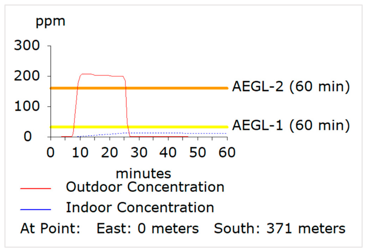
The receptor location was defined at a distance of 371 m from the release source, corresponding to the location of the Veternik residential care facility. In ALOHA (version 5.4.7), the receptor was defined at East 0 m and South 371 m relative to the release source. In the ALOHA Threat-at-Point calculation, this receptor was used as the downwind point for which the outdoor and indoor concentration–time estimates were generated. This facility was selected as a representative receptor because it accommodates individuals who may experience reduced mobility and increased evacuation challenges during emergency situations.
The resulting concentration–time series serves as the primary input for the proposed dynamic exposure assessment framework and enables the estimation of both accumulated exposure and the duration of exposure above the selected AEGL-2 reference threshold. The present implementation illustrates the proposed framework using a single representative receptor located at a facility accommodating a vulnerable population. The framework itself is not restricted to a single receptor and can be applied to multiple receptor locations using the corresponding location-specific concentration–time profiles.
3.3. Meteorological Conditions
Meteorological input parameters were derived from observational data for January 2024 obtained from the Republic Hydrometeorological Service of Serbia, which provides publicly available meteorological records at the national level [
34].
The procedure for selecting representative meteorological conditions follows the methodology previously developed by the authors [
6], ensuring consistency with the original hazard assessment framework. Three meteorological scenarios are considered, corresponding to the worst-case (WC), best-case (BC), and most probable (MP) dispersion conditions. The WC scenario combines the maximum atmospheric temperature with the minimum wind speed, whereas the BC scenario combines the minimum atmospheric temperature with the maximum wind speed. For these scenarios, wind direction is selected according to the scenario-definition procedure established in [
6]. For the remaining meteorological variables, representative values are derived from their monthly distributions. For the MP scenario, the most frequent values of the meteorological variables are used to represent the prevailing monthly conditions.
Consistent with the temporal settings adopted in the previous methodology [
6], the 15th day of the month and 14:00 h are used as standardized temporal inputs for the simulations. These values serve as scenario-definition inputs and should not be interpreted as indicating that the simulated release occurred on a specific observed accident date. In the original methodology, 14:00 h was selected as the assumed most probable time of ammonia transportation in the vicinity of the exposed facility, while the 15th day was adopted as a representative reference date for the monthly meteorological scenarios. Since the meteorological parameters were derived from monthly statistical distributions rather than from a specific observation date, the selected calendar date serves only as a consistent temporal reference.
January is used for the present demonstration because the previous investigation showed a qualitatively consistent pattern of simulated ammonia dispersion across the months considered, despite seasonal variation in meteorological conditions [
6]. The present study demonstrates the proposed dynamic exposure assessment framework under a defined set of atmospheric conditions rather than exploring seasonal variability in atmospheric dispersion. Accordingly, a single-month dataset is considered sufficient for defining the meteorological scenarios used in the present analysis.
The selected parameters include atmospheric temperature, wind speed and direction, cloudiness, atmospheric stability class, and relative humidity. These inputs are subsequently used to define the atmospheric dispersion conditions within the ALOHA model. The resulting WC, BC, and MP scenarios used in the present study are summarized in
Table 1.
The WC, BC, and MP scenarios characterize the meteorological conditions considered in the underlying dispersion analysis. The concentration–time profile used for the subsequent dynamic exposure calculations was generated specifically using the WC scenario presented in
Table 1.
3.4. ALOHA Dispersion Modeling Configuration
Atmospheric dispersion modeling is performed using the ALOHA (Areal Locations of Hazardous Atmospheres, version 5.4.7) software under non-ignited toxic-release conditions. The principal source, site, release, and model parameters used in the present study are summarized in
Table 2.
ALOHA also provides an indoor concentration estimate based on the specified building air-exchange characteristics. In the present framework, however, the dynamic exposure calculations are based on the outdoor concentration profile at the receptor.
For the selected source configuration, ALOHA calculated a maximum average sustained release rate of 81.5 kg/min and a total released mass of 1520 kg, with the release duration limited by the software to 1 h. The release was modeled as a gas–aerosol mixture (two-phase flow), and ALOHA applied the Heavy Gas dispersion model. The WC meteorological scenario defined in
Table 1 was used to generate the receptor-specific concentration–time profile employed in the subsequent dynamic exposure analysis.
3.5. Generated Concentration–Time Profile
The ALOHA simulation produces both spatial toxic threat zones and time-dependent concentration estimates at the selected receptor. These outputs characterize the spatial and temporal behavior of the modeled ammonia release and provide the hazard information used in the subsequent dynamic exposure assessment.
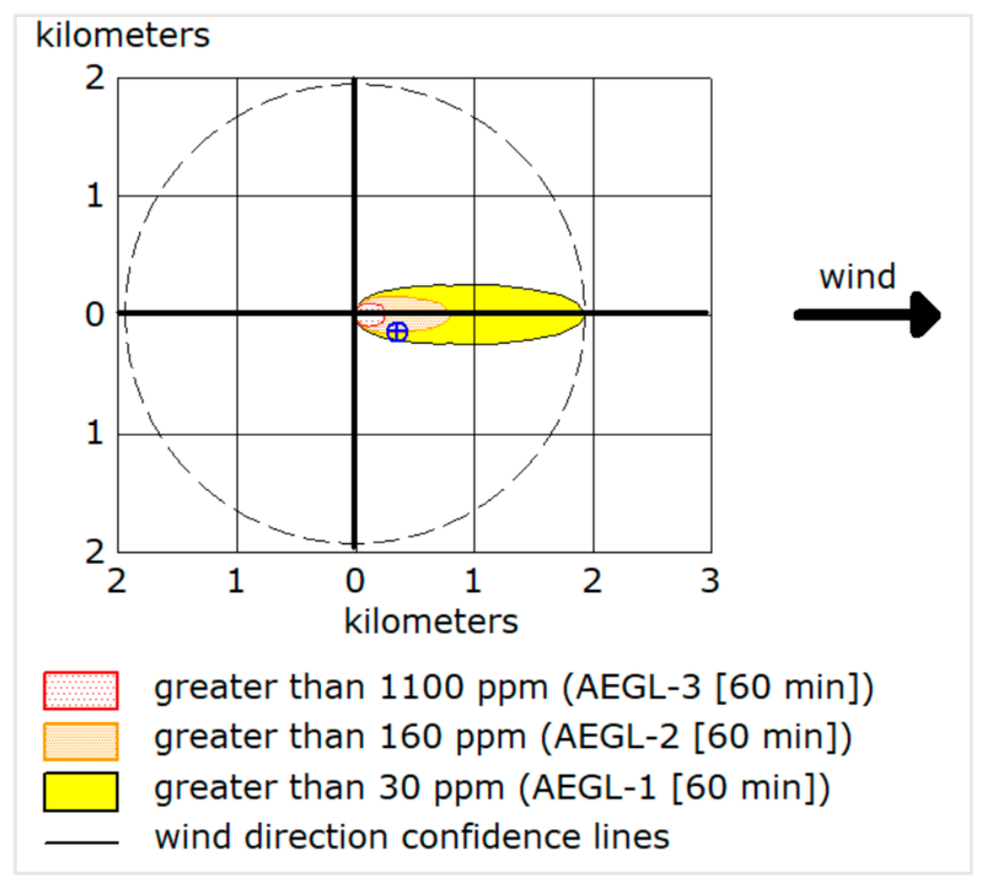
Figure 1 presents the toxic threat zones generated under the WC meteorological scenario and shows the position of the selected receptor relative to the modeled plume. For the 60-min AEGL reference levels used by ALOHA, the modeled threat-zone distances along the plume were 237 m for AEGL-3 (1100 ppm), 797 m for AEGL-2 (160 ppm), and 1.9 km for AEGL-1 (30 ppm). The spatial distribution of the toxic plume indicates that the selected receptor is located within the affected area under the considered meteorological conditions.
Figure 2 shows the concentration–time output generated by ALOHA at the selected receptor (East 0 m, South 371 m). The outdoor concentration rises rapidly after the arrival of the plume, reaches an approximately 200 ppm plateau, and subsequently declines. The accompanying ALOHA Threat-at-Point output reports a maximum outdoor concentration of 204 ppm at this receptor, while the corresponding maximum indoor concentration is 12.5 ppm for the specified sheltered, single-storied building configuration. The approximately 200 ppm plateau subsequently used in the reconstructed concentration–time profile therefore represents a graphical approximation of the ALOHA output and is consistent with the reported maximum outdoor concentration of 204 ppm.
The dynamic exposure calculations in the present study are based on the outdoor concentration profile at the selected receptor. Because the ALOHA concentration–time output was available graphically rather than as an exportable numerical time series, the outdoor profile was subsequently reconstructed using characteristic time–concentration points extracted from the graphical output. The ALOHA Text Summary was used to verify the reported maximum outdoor concentration at the receptor. The reconstruction procedure and the corresponding numerical values used for exposure integration are presented in
Section 5.1.
The temporal structure of the outdoor concentration profile, including its rising phase, elevated concentration plateau, and subsequent decay, provides the basis for examining the interaction between evacuation completion time and accumulated exposure in the subsequent scenario-based analysis.
4. Scenario Analysis Framework
This section defines the analytical setup used to evaluate the impact of evacuation delay on exposure outcomes. The analysis is conducted through a set of controlled evacuation scenarios applied to a fixed hazard configuration, enabling direct comparison of exposure metrics under varying response conditions.
4.1. Definition and Temporal Interpretation of Evacuation Scenarios
Three evacuation scenarios are defined to examine the effect of vulnerability-related evacuation delay on accumulated exposure. In accordance with the general formulation presented in
Section 2.3, the non-vulnerability-related components of evacuation time are held constant across all scenarios, while only the additional vulnerability-related delay,
, is varied.
For the present demonstration, a baseline evacuation completion time of 10 min is assumed for Scenario S0. This value represents the combined duration of hazard alert, baseline mobilization, and movement to safety under standard response conditions. The individual components are not assigned separate numerical values in the present demonstration, as the purpose of the scenario design is to isolate the effect of additional vulnerability-related delay rather than to reproduce the detailed evacuation process of a specific facility.
The additional vulnerability-related delays are introduced as illustrative scenario parameters representing progressively delayed response conditions rather than empirically calibrated evacuation times for the specific facility. Accordingly, Scenario S0 (Baseline) assumes , Scenario S1 (Moderate Delay) assumes min, and Scenario S2 (Severe Delay) assumes min.
The resulting evacuation completion times are therefore 10 min for Scenario S0, 20 min for Scenario S1, and 35 min for Scenario S2. Consequently, the scenarios represent progressively longer accumulated exposure periods measured from release onset until evacuation completion.
Accumulated exposure is therefore evaluated over the following time intervals:
Scenario S0: 0–10 min;
Scenario S1: 0–20 min;
Scenario S2: 0–35 min.
These intervals represent accumulated exposure periods rather than independent exposure windows. Accordingly, Scenarios S1 and S2 are evaluated from release onset over the intervals 0–20 min and 0–35 min, respectively, rather than as incremental exposure periods of 10–20 min and 20–35 min. The additional exposure associated with evacuation delay is analysed separately through marginal interval contributions, enabling the identification of the portions of the concentration–time profile that contribute most strongly to accumulated exposure.
This temporal interpretation enables the analysis of how evacuation delay interacts with the dynamic structure of the concentration–time profile and provides the basis for evaluating both accumulated exposure and the marginal contribution of individual delay intervals.
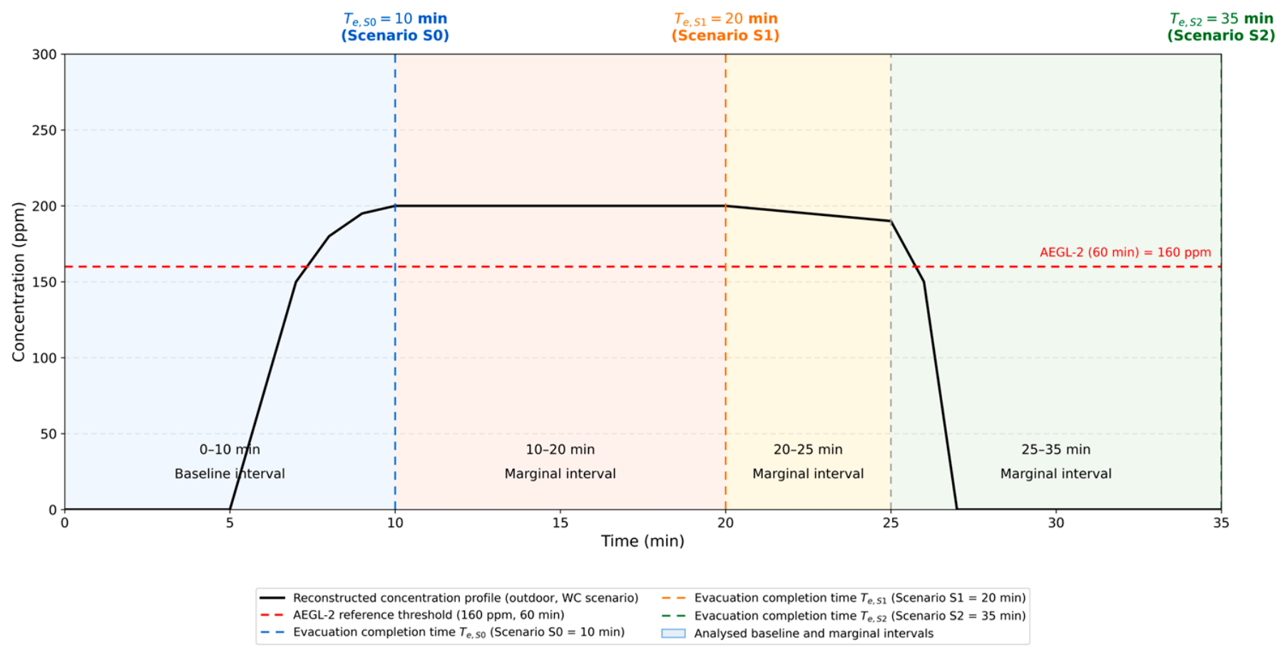
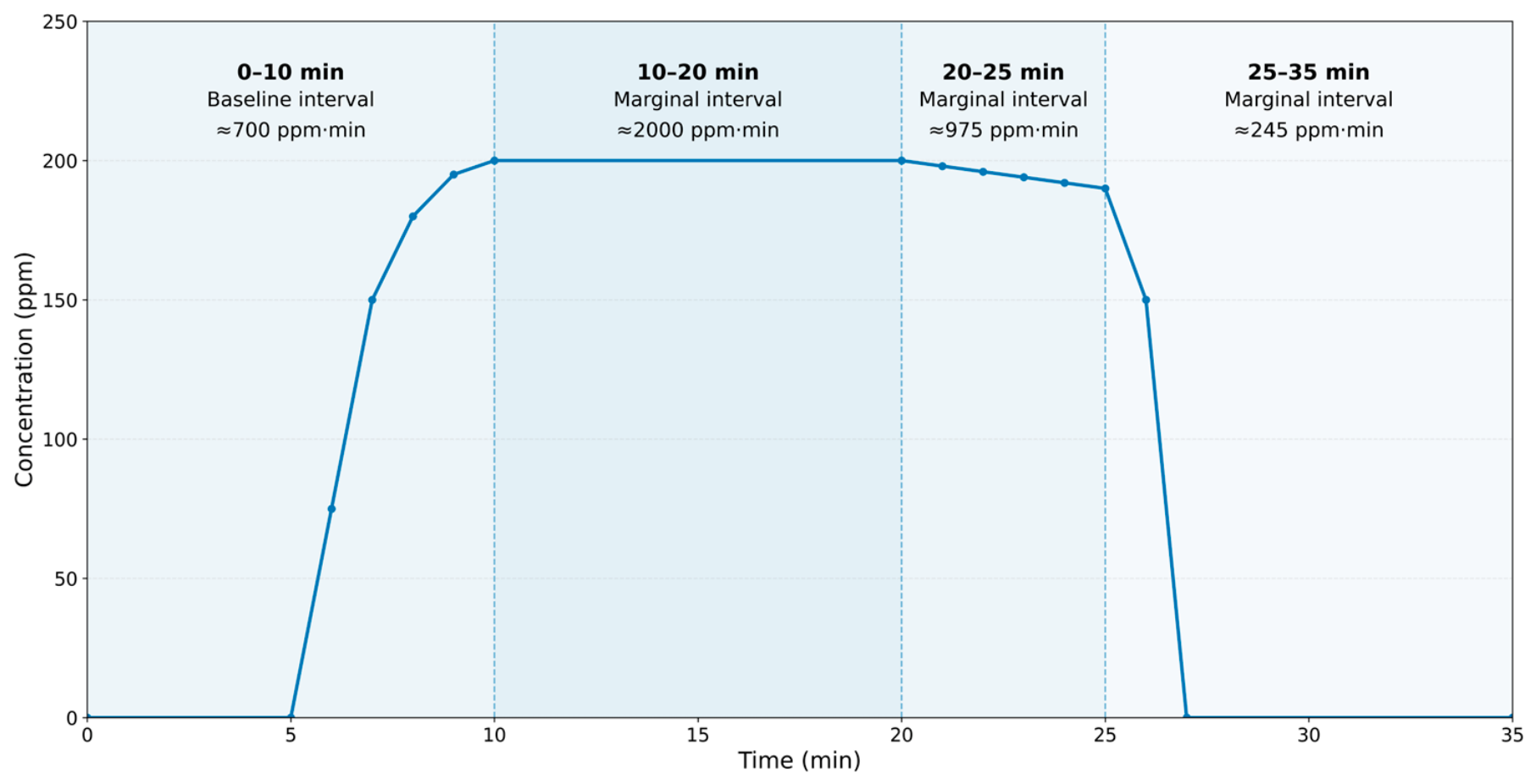
The reconstructed concentration–time profile together with the scenario-specific evacuation completion times and the analysed baseline and marginal intervals is presented in
Figure 3.
4.2. Exposure Metrics and Analytical Objective
For each evacuation scenario, two complementary exposure metrics are evaluated:
Accumulated exposure, representing the integrated concentration from release onset until evacuation completion;
Time above the AEGL-2 reference threshold, representing the duration for which the reconstructed concentration exceeds the selected 60-min AEGL-2 reference level within the scenario-specific exposure period.
Together, these metrics characterize both the integrated concentration over the exposure period and the duration of concentration exceedance above the selected reference threshold. The AEGL-2 value is used here as a fixed reference level for temporal exceedance characterization, consistent with the interpretation defined in
Section 2.4.
The analysis is designed to examine how evacuation delay influences exposure outcomes under identical hazard conditions and to evaluate the extent to which these outcomes depend on the temporal interaction between evacuation timing and the concentration–time profile. Particular attention is given to identifying the time intervals that contribute most strongly to accumulated exposure and AEGL-2 exceedance duration.
Although demonstrated here for ammonia, the analytical structure is not inherently substance-specific and can be applied to other toxic-release scenarios provided that an appropriate time-dependent concentration profile is available. Threshold-based interpretation would additionally require an appropriate substance-specific health-based reference criterion.
5. Results and Dynamic Exposure Analysis
This section presents the results of the dynamic exposure assessment for the three evacuation-delay scenarios. The analysis progresses from accumulated exposure and interval-specific contributions to AEGL-2 exceedance duration, the identification of critical evacuation windows, and an assessment of the robustness of these findings to variations in the reconstructed concentration–time profile.
5.1. Impact of Evacuation Delay on Accumulated Exposure
The accumulated exposure results were obtained for the three evacuation-delay scenarios defined in
Section 4.1. Exposure was calculated as the time integral of concentration from release onset until the scenario-specific evacuation completion time, following the formulation introduced in
Section 2.2. As defined in
Section 4.1, the assumed evacuation completion times are 10 min for Scenario S0, 20 min for Scenario S1, and 35 min for Scenario S2.
ALOHA provides the concentration–time profile graphically but does not provide a directly exportable numerical time series for the analysed Threat at Point output. Therefore, the concentration–time profile used in the exposure calculations was reconstructed from characteristic points identified from the graphical output. Accordingly, the reconstructed concentration values should be interpreted as approximate inputs for the methodological demonstration rather than as directly exported numerical ALOHA data.
The reconstructed concentration profile was represented by piecewise-linear segments, and accumulated exposure was approximated by trapezoidal integration over consecutive reconstructed time points:
where
and
represent reconstructed concentration values at consecutive time points, and
denotes the corresponding time interval.
The reconstructed concentration–time points used for trapezoidal integration are presented in
Table 3.
The integration therefore uses the consecutive time intervals defined by the reconstructed points in
Table 3, with interval lengths ranging from 1 to 10 min, reflecting the temporal structure of the graphical profile.
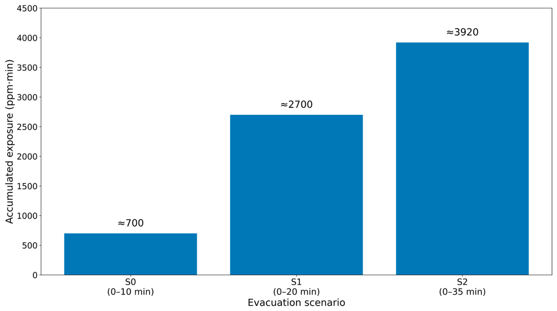
Based on the reconstructed concentration profile, accumulated exposure was estimated for each evacuation scenario. The values are presented in
Table 4 and
Figure 4 represent exposure accumulated from release onset until the corresponding evacuation completion time.
Accumulated exposure increases across the progressively delayed evacuation scenarios because each scenario extends the period over which exposure is integrated. Scenario S2 therefore produces the highest accumulated exposure, followed by Scenario S1 and Scenario S0. This ordering is consistent with the exposure formulation, in which exposure accumulates from release onset until the scenario-specific evacuation completion time.
To examine how different portions of the evacuation period contribute to the overall exposure burden, exposure contributions were additionally evaluated over the baseline and successive marginal time intervals using the same trapezoidal integration procedure. The resulting interval contributions are presented in
Table 5.
The interval-based analysis shows that the largest marginal increase in accumulated exposure occurs during the 10–20 min interval, which coincides with the peak concentration plateau of the reconstructed concentration–time profile. The subsequent 20–25 min interval also contributes substantially to accumulated exposure, although its contribution is smaller because concentrations gradually decline during this period. In contrast, the late-stage 25–35 min interval contributes only modestly to accumulated exposure as the concentration profile enters its decay phase.
These differences follow directly from integrating a time-varying concentration profile over successive exposure intervals: additional evacuation time occurring during periods of higher concentration contributes more to accumulated exposure than additional time occurring during periods of lower concentration. In the present demonstration, the 10–20 min interval therefore represents the period in which additional evacuation delay produces the largest marginal increase in accumulated exposure. This interval-specific interpretation provides the basis for identifying evacuation periods of particular relevance in the subsequent analysis.
5.2. Time Above the AEGL-2 Reference Threshold
In addition to accumulated exposure, the duration for which ammonia concentrations exceeded the AEGL-2 reference threshold was evaluated for each evacuation scenario. Using the reconstructed outdoor WC concentration–time profile presented in
Section 5.1, the time spent above the selected threshold was estimated within the corresponding exposure period of each scenario.
In the present analysis, the 60-min AEGL-2 value for ammonia (160 ppm) is used as a fixed reference threshold for temporal exceedance characterization. It is not applied as a duration-specific toxicological classification for the shorter exposure periods considered in the evacuation scenarios. Rather, the threshold provides a consistent reference level for examining how evacuation timing affects the duration of exposure to elevated ammonia concentrations.
Because the concentration–time profile was reconstructed from the graphical ALOHA output, the reported exceedance durations should be interpreted as approximate estimates supporting the methodological demonstration rather than as exact exceedance durations. Based on linear interpolation of the reconstructed profile, the concentration exceeds the selected AEGL-2 reference threshold from approximately 7–8 min until approximately 25–26 min, corresponding to a total exceedance duration of approximately 18.4 min for the reconstructed concentration–time profile.
The durations above the AEGL-2 reference threshold obtained for the analysed evacuation scenarios are presented in
Table 6.
The duration above the AEGL-2 reference threshold increases across the progressively delayed evacuation scenarios because the extended exposure periods in Scenarios S1 and S2 overlap with portions of the concentration profile that remain above the selected reference threshold. Scenario S2 therefore produces the longest exceedance duration, followed by Scenario S1 and Scenario S0. This ordering reflects the interaction between scenario-specific evacuation completion times and the temporal evolution of the reconstructed concentration profile.
To further examine the influence of evacuation timing, the contribution of the baseline and successive marginal time intervals to the overall AEGL-2 exceedance duration was analysed separately. The corresponding interval-specific exceedance durations are presented in
Table 7.
The interval-based analysis shows that the largest contribution to AEGL-2 exceedance duration occurs during the 10–20 min interval, throughout which the reconstructed concentration remains above the selected reference threshold. The subsequent 20–25 min interval also contributes substantially because concentrations remain above the selected AEGL-2 reference threshold throughout this period. In contrast, the late-stage 25–35 min interval contributes only marginally, as concentrations fall below the reference threshold between approximately 25 and 26 min.
These results indicate that evacuation timing influences not only accumulated exposure but also the duration for which concentrations remain above the selected AEGL-2 reference threshold within each scenario-specific exposure period. The 10–20 min interval makes the largest interval-specific contribution to accumulated exposure and also accounts for the longest AEGL-2 exceedance duration among the analysed intervals, although the two metrics characterize different aspects of the concentration–time profile. The broader implications of these temporal differences for understanding the interaction between evacuation timing and hazard evolution are examined in the following section.
5.3. Temporal Effects of Evacuation Delay and Critical Evacuation Windows
Figure 5 illustrates how different phases of the concentration–time profile contribute to accumulated exposure through the marginal exposure contributions associated with successive time intervals.
The results demonstrate that the influence of evacuation delay on exposure cannot be explained solely by the duration of the delay itself. Although accumulated exposure increases with evacuation delay and reaches its highest value in Scenario S2, the contribution of individual delay intervals varies substantially depending on their position within the concentration–time profile.
The marginal exposure analysis presented in
Section 5.1 indicates that the largest increase in accumulated exposure occurs during the 10–20 min interval. This period coincides with the peak concentration plateau, during which concentrations remain close to their maximum values. Consequently, evacuation delay occurring during this interval produces the largest marginal contribution to accumulated exposure among the analysed intervals.
In contrast, the additional delay associated with the 25–35 min interval produces a comparatively small increase in exposure despite representing an equally long interval. At this stage, concentrations have entered the later stages of the decay phase and therefore contribute less to accumulated exposure, while only a small portion of the interval remains above the selected AEGL-2 reference threshold. As a result, the contribution of additional evacuation delay depends not only on how long evacuation is delayed, but also on when the delay occurs relative to the evolution of the concentration field.
A similar pattern is observed in the AEGL-based analysis presented in
Section 5.2. The largest interval-specific contribution to the duration above the selected AEGL-2 reference threshold occurs during the 10–20 min interval. The following 20–25 min interval also remains above the selected AEGL-2 reference threshold and therefore contributes substantially to the exceedance duration, whereas the late decay phase after approximately 25–26 min contributes only marginally.
These findings reflect the interaction between evacuation timing and the temporal structure of the concentration profile. Additional evacuation time occurring during periods of elevated concentration produces greater increases in accumulated exposure than additional time occurring during later stages of the concentration decay phase. In the analysed scenario, the 10–20 min interval can therefore be identified as a critical evacuation window, as additional evacuation delay during this period produces the largest marginal increase in accumulated exposure and the largest interval-specific contribution to the duration above the selected AEGL-2 reference threshold.
The results further suggest that conventional static hazard representations may be insufficient for evaluating exposure conditions during toxic release events. While static hazard maps indicate the spatial extent of hazardous zones, they do not capture the temporal evolution of concentration levels or the effects of delayed evacuation. The proposed framework addresses this limitation by explicitly linking hazard dynamics with evacuation timing and vulnerability-related response constraints.
This capability is particularly relevant for vulnerable population groups whose evacuation may be delayed due to mobility limitations, reduced response capacity, or the need for external assistance. Under such conditions, even relatively short delays may extend the exposure period into portions of the concentration–time profile characterized by elevated concentrations, resulting in substantial increases in accumulated exposure and the duration above the selected AEGL-2 reference threshold. Incorporating these temporal effects into exposure assessment can therefore support more inclusive emergency planning, targeted evacuation support measures, and improved protection of vulnerable populations during hazardous-material incidents.
5.4. Sensitivity Analysis of the Reconstructed Concentration Profile
Because the concentration–time profile used in the exposure calculations was reconstructed from the graphical ALOHA output, a sensitivity analysis was conducted to evaluate the extent to which variations in the reconstructed concentration values could affect the calculated exposure metrics and their interpretation. The analysis was designed specifically to assess the robustness of the main findings under structured perturbations of the reconstructed concentration values. Its purpose is to evaluate the robustness of the comparative scenario ordering and the principal temporal pattern rather than to quantify model-form uncertainty or provide a formal probabilistic uncertainty quantification.
The reconstructed concentration values presented in
Table 3 were systematically perturbed by
,
, and
relative to the unperturbed reconstructed profile. These perturbation levels provide a structured range of concentration-magnitude variations for robustness testing. For each perturbation level, the concentration at each reconstructed time point was calculated as:
where
represents the unperturbed reconstructed concentration at time point
,
represents the perturbed concentration, and
denotes the applied perturbation level (−0.15, −0.10, −0.05, 0, +0.05, +0.10, or +0.15). Concentration values equal to zero were retained as zero. The temporal structure of the reconstructed profile was kept unchanged, thereby isolating the effect of variations in concentration magnitude.
For each perturbed profile, accumulated exposure was recalculated using the same trapezoidal integration procedure applied in
Section 5.1. Calculations were performed for the accumulated exposure periods associated with Scenarios S0, S1, and S2, as well as for the baseline and marginal time intervals used to evaluate the temporal contribution of evacuation delay. The resulting values are presented in
Table 8.
The sensitivity analysis shows that changes in reconstructed concentration magnitude affect the absolute accumulated exposure values, as expected. However, the relative ordering of the evacuation scenarios remains unchanged across all tested perturbations, with Scenario S2 consistently producing the highest accumulated exposure, followed by S1 and S0. Similarly, the 10–20 min interval remains the largest marginal contributor under every tested concentration profile. These results indicate that the principal temporal pattern identified in
Section 5.1 remains stable across the tested perturbation range.
Sensitivity was also evaluated for the AEGL-2 exceedance metric. For each perturbed profile, the times at which the concentration crossed the fixed AEGL-2 reference threshold of 160 ppm were recalculated using linear interpolation between consecutive reconstructed time points. The resulting exceedance durations for each evacuation scenario and for the baseline and marginal time intervals are presented in
Table 9.
The AEGL-2 exceedance metric responds differently to concentration perturbations than accumulated exposure because exceedance duration depends on the position of the concentration profile relative to the fixed reference threshold. Under the unperturbed reconstructed profile, the AEGL-2 reference threshold is exceeded from approximately 7–8 min to approximately 25–26 min. Across the tested perturbations, both the onset and the end of threshold exceedance shift as the reconstructed concentration values change, with the resulting sensitivity values presented in
Table 9.
Despite these variations, the qualitative interpretation remains stable. Scenario S2 consistently produces the longest AEGL-2 exceedance duration, followed by S1 and S0. The 10–20 min interval remains the largest interval-specific contributor to AEGL-2 exceedance duration under all tested perturbations, while the 20–25 min interval remains entirely above the selected reference threshold. The greatest variation occurs near the beginning and end of the threshold-exceedance period, where changes in reconstructed concentration magnitude shift the interpolated threshold-crossing times.
Overall, the sensitivity analysis demonstrates that variations in the magnitude of the reconstructed ALOHA concentration–time profile affect the absolute values of both accumulated exposure and AEGL-2 exceedance duration but do not alter the principal qualitative findings of the analysis. In particular, the ordering of evacuation scenarios remains unchanged, and the 10–20 min interval consistently produces the largest marginal increase in accumulated exposure and the largest interval-specific contribution to AEGL-2 exceedance duration across the full perturbation range. The identification of this interval as the critical evacuation window in the analysed scenario is therefore robust to the tested concentration-magnitude perturbations. The results also show that threshold-crossing times and the resulting AEGL-2 exceedance durations vary with changes in the reconstructed concentration values, particularly near the beginning and end of the threshold-exceedance period.
6. Discussion
The results demonstrate that exposure outcomes during toxic release events are strongly influenced by evacuation dynamics and cannot be fully characterized through conventional static hazard representations alone. Traditional consequence-based approaches commonly delineate hazard zones using concentration thresholds and spatial impact distances [
7,
8,
13]. While such approaches provide valuable information regarding the spatial extent of hazardous conditions, they do not explicitly account for the accumulation of exposure over time while individuals remain within the affected area.
The proposed framework addresses this limitation by conceptualizing exposure as a cumulative process extending from release onset until evacuation completion. Under identical hazard conditions, progressively delayed evacuation scenarios produced progressively higher accumulated exposure outcomes, confirming that evacuation timing directly influences the resulting exposure. These findings support the growing recognition that exposure assessment should incorporate temporal dynamics in addition to spatial hazard characterization [
20,
24].
A key finding of the study is that the effect of evacuation delay on accumulated exposure depends on the temporal position of the delay within the evolving concentration profile. Although accumulated exposure increased progressively from Scenario S0 to Scenario S2, the marginal contribution of additional delay varied substantially across different portions of the concentration–time profile. The interval analysis revealed that the largest increase in accumulated exposure occurred during the 10–20 min period, corresponding to the concentration plateau where ammonia concentrations remained near their maximum values. In contrast, the additional delay occurring during the late decay phase contributed comparatively little to the overall accumulated exposure. These findings indicate that additional evacuation time does not contribute uniformly to exposure and that the temporal position of the delay is as important as its duration.
This behavior is consistent with previous studies highlighting the importance of interactions between hazard evolution and evacuation processes [
24,
25,
26]. Dynamic approaches combining toxic gas dispersion and evacuation modelling have demonstrated the importance of considering the evolving concentration field together with evacuation processes [
22,
23], while more recent work has explicitly examined how evacuation risk changes over time during accidental toxic gas releases [
27]. The present framework provides a complementary analytical perspective by directly quantifying accumulated exposure up to scenario-specific evacuation completion times and explicitly distinguishing total accumulated exposure from the contributions of successive time intervals. This distinction provides additional insight into how specific portions of evacuation delay contribute to accumulated exposure and enables the identification of periods in which additional delay has the greatest influence on the exposure measures considered.
The analysis of AEGL-2 exceedance duration further supports this temporal interpretation. The longest exceedance duration was observed in the most delayed evacuation scenario. The interval-based analysis showed that the 10–20 min interval made the largest interval-specific contribution, while the 20–25 min interval also contributed substantially because concentrations remained above the selected AEGL-2 reference threshold throughout this period. In contrast, the late decay phase contributed only marginally to threshold-exceedance duration. In the analysed scenario, the 10–20 min interval can therefore be identified as a critical evacuation window because additional evacuation delay during this period produces the largest marginal increase in accumulated exposure and the largest interval-specific contribution to AEGL-2 exceedance duration.
The AEGL-based results should, however, be interpreted according to the threshold formulation adopted in this study. The 60-min AEGL-2 concentration for ammonia is used as a fixed reference threshold for temporal exceedance characterization and not as a duration-specific toxicological classification for the shorter scenario-specific exposure periods. Similarly, accumulated exposure expressed as concentration integrated over time should be interpreted as an exposure metric rather than as a direct predictor of health effects. Concentration–duration relationships are endpoint- and substance-dependent, and simple concentration–time relationships are not universally applicable for toxicological response assessment [
18]. Accordingly, the accumulated exposure and threshold-exceedance metrics used here are intended to support comparative analysis of evacuation scenarios under a common hazard profile.
The findings are particularly relevant for vulnerable populations. Individuals with disabilities, reduced mobility, advanced age, or other functional limitations may experience evacuation constraints that increase the time required to reach safety. Previous research has shown that functional limitations can affect evacuation performance and has highlighted the importance of considering the temporal dimension of evacuation for populations with different functional capabilities [
31]. Under such conditions, even relatively short delays may substantially increase accumulated exposure if they coincide with periods of elevated concentration. Consequently, the results suggest that emergency planning strategies should consider not only whether evacuation occurs, but also when evacuation occurs relative to the temporal evolution of the hazard. For populations requiring assistance, protective-action decisions may also involve a trade-off between the time needed to organize safer assisted evacuation and the additional exposure that may accumulate while evacuation is delayed. The proposed framework does not prescribe whether evacuation, sheltering, or another protective action should be selected, but provides an additional temporal exposure perspective that can inform such decisions alongside operational, medical, and safety considerations.
Although the demonstration case is based on an ammonia release scenario generated using ALOHA, the conceptual framework itself is not substance-specific. Because the methodology relies on time-dependent concentration profiles and evacuation timing, it can in principle be applied to other toxic release scenarios whenever an appropriate concentration–time profile is available. Threshold-based characterization would additionally require an appropriate substance-specific reference criterion. This characteristic supports the potential applicability of the framework across different hazardous substances, release conditions, and emergency-planning contexts.
The broader applicability of the proposed framework has practical implications for emergency planning. In an operational emergency-planning workflow, the framework could be applied after a dispersion model has generated receptor-specific concentration–time profiles. For relevant facilities or receptor locations, planners could combine these profiles with scenario-specific evacuation completion times representing population groups with different evacuation requirements. The resulting accumulated exposure, AEGL-2 exceedance duration, and interval-specific contributions could then be used to identify periods in which delayed evacuation produces the greatest increase in the exposure measures considered. This information would not replace established protective-action guidance or operational decision-making, but could complement conventional consequence modelling by highlighting the temporal consequences of delayed response. This may be particularly relevant for facilities accommodating vulnerable populations, such as hospitals, residential care facilities, schools, and similar institutions, where evacuation may require additional time and external assistance. Incorporating time-dependent exposure analysis into emergency planning protocols may therefore support the identification of critical evacuation windows, evacuation prioritization, and the evaluation of protective measures under toxic release conditions.
The present study is subject to several limitations. First, the framework is demonstrated using a single receptor location and a concentration–time profile reconstructed from graphical ALOHA output rather than directly exported numerical data. Consequently, the reported exposure values should be interpreted as approximate estimates supporting methodological demonstration rather than precise exposure quantification. The sensitivity analysis showed that perturbations of in the reconstructed concentration magnitude affected the absolute values of accumulated exposure and AEGL-2 exceedance duration but did not alter the ordering of the evacuation scenarios or the identification of the 10–20 min interval as the critical evacuation window in the analysed scenario. This provides evidence that the principal temporal interpretation is robust to the tested concentration-magnitude perturbations.
Second, the dynamic exposure calculations are based on the outdoor concentration profile at a fixed receptor and do not model individual movement trajectories or transitions between outdoor and indoor environments during evacuation. ALOHA also provides an indoor concentration estimate based on specified building air-exchange characteristics; however, indoor exposure is not incorporated into the present dynamic calculations. The framework itself is not restricted to a single receptor and can, in principle, be applied to multiple receptor locations using corresponding location-specific concentration–time profiles, but spatially distributed populations and dynamic evacuation routes are not explicitly modelled in the present demonstration. Finally, the framework is demonstrated using a single ammonia release configuration and one meteorological scenario for the dynamic exposure analysis. Additional applications across different substances, release characteristics, meteorological conditions, receptor configurations, and evacuation settings would provide further evidence regarding the generalizability of the proposed approach.
Future work could further extend the framework by comparing its application across different facility types accommodating populations with specific evacuation or assistance requirements. In addition, integrating time-dependent exposure assessment with broader consequence and economic analyses could support the comparative evaluation of protective measures and longer-term risk-reduction strategies. Such an extension would broaden the framework from the temporal assessment of evacuation-related exposure toward a more comprehensive evaluation of alternative interventions for reducing the consequences of toxic release events.
7. Conclusions
This study proposed a dynamic exposure assessment framework that integrates time-dependent concentration profiles with scenario-specific evacuation completion times to evaluate toxic exposure under delayed evacuation conditions, with particular emphasis on vulnerability-related response delays.
The results demonstrated that evacuation timing can substantially influence accumulated exposure because exposure is evaluated from release onset until evacuation completion. Under identical hazard conditions, progressively delayed evacuation scenarios produced progressively higher accumulated exposure values and longer durations above the selected AEGL-2 reference threshold. In the present demonstration, the vulnerability-related delays were introduced as illustrative scenario parameters rather than empirically calibrated evacuation times, allowing the temporal effect of delayed evacuation to be examined under controlled conditions. Accordingly, the numerical results should be interpreted as illustrative scenario outputs rather than empirical predictions of exposure under a specific real-world incident.
The analysis further showed that the contribution of additional evacuation delay depends on its temporal position within the evolving concentration profile. In the analysed scenario, the 10–20 min interval was identified as a critical evacuation window because it produced the largest marginal increase in accumulated exposure and the largest interval-specific contribution to AEGL-2 exceedance duration. These findings emphasize that the exposure contribution of additional evacuation delay depends not only on its duration but also on its temporal position relative to the evolving concentration profile.
The sensitivity analysis showed that the principal qualitative findings remained stable under structured perturbations of the reconstructed concentration profile. Across the tested range, the ordering of accumulated exposure among the evacuation scenarios remained unchanged, and the 10–20 min interval consistently produced the largest marginal exposure contribution. Although threshold-crossing times and AEGL-2 exceedance durations varied with changes in reconstructed concentration magnitude, the overall temporal interpretation remained stable.
The study also demonstrated the value of distinguishing between accumulated exposure and interval-specific contributions. While accumulated exposure represents the total exposure burden from release onset until evacuation completion, interval-based analysis identifies the portions of the exposure period that contribute most strongly to that burden. Combined with the AEGL-2 exceedance metric, this distinction provides additional information on the interaction between hazard evolution and evacuation timing and may support the evaluation of evacuation priorities and protective measures.
Although demonstrated using an ammonia-release scenario modeled in ALOHA, the framework is not inherently substance-specific and can, in principle, be applied to other toxic release scenarios whenever an appropriate time-dependent concentration profile is available. Threshold-based interpretation additionally requires an appropriate substance-specific health-based reference criterion. The ammonia-specific parameters and AEGL values used in the present demonstration should therefore not be directly transferred to other substances or release conditions.
Future research should further evaluate and validate the framework using empirically informed evacuation times, multiple receptor locations, spatially distributed populations, realistic movement and evacuation-route dynamics, and indoor–outdoor exposure transitions. Applications involving additional hazardous substances, release characteristics, and meteorological conditions would provide further evidence regarding the robustness and broader applicability of the proposed approach. Such developments could strengthen the practical use of time-dependent exposure assessment in emergency planning, particularly for populations requiring additional evacuation time or assistance.
Author Contributions
Conceptualization, J.S., T.V. and S.P.; methodology, J.S., T.V. and S.P.; formal analysis, J.S. and T.V.; investigation, J.S. and C.L.; data curation, J.S. and C.L.; visualization, J.S. and C.L.; validation, T.V., C.L., Ž.Z. and S.P.; writing—original draft preparation, J.S.; writing—review and editing, T.V., C.L., Ž.Z. and S.P.; supervision, T.V., Ž.Z. and S.P.; project administration, Ž.Z. All authors have read and agreed to the published version of the manuscript.
Funding
This research received no external funding.
Institutional Review Board Statement
Not applicable.
Informed Consent Statement
Not applicable.
Data Availability Statement
The data supporting the findings of this study are contained within the article. The meteorological input parameters, ALOHA simulation configuration, reconstructed concentration–time values, accumulated exposure estimates, and AEGL-2 exceedance calculations are presented in the manuscript. Additional supporting information related to the ALOHA graphical outputs and intermediate calculation files can be made available from the corresponding author upon reasonable request.
Acknowledgments
The authors acknowledge the support of the Ministry of Science, Technological Development and Innovation of the Republic of Serbia (Contract No. 451-03-34/2026-03/200156) and the Faculty of Technical Sciences, University of Novi Sad, through the project “Scientific and Artistic Research Work of Researchers in Teaching and Associate Positions at the Faculty of Technical Sciences, University of Novi Sad 2026” (No. 01-3609/1).
Conflicts of Interest
The authors declare no conflicts of interest.
Abbreviations
The following abbreviations are used in this manuscript:
| AEGL | Acute Exposure Guideline Level |
| ALOHA | Areal Locations of Hazardous Atmospheres |
| GIS | Geographic Information System |
| MP | Most Probable |
| BC | Best Case |
| WC | Worst Case |
References
- Torretta, V.; Rada, E.C.; Schiavon, M.; Viotti, P. Decision support systems for assessing risks involved in transporting hazardous materials: A review. Saf. Sci. 2017, 92, 1–9. [Google Scholar] [CrossRef] [Scilit]
- Fan, T.; Chiang, W.-C.; Russell, R.A. Modeling urban hazmat transportation with road closure consideration. Transp. Res. Part D Transp. Environ. 2015, 35, 104–115. [Google Scholar] [CrossRef] [Scilit]
- Teng, L.; Ling, P.; Zhao, C.; Zhang, Z.; Liu, B.; Li, J.; Yin, P.; Li, Z.; Jiang, L. A data-driven risk assessment framework for ammonia pipelines: Insights from 232 accident cases (1970–2023). J. Pipeline Sci. Eng. 2025, 6, 100388. [Google Scholar] [CrossRef] [Scilit]
- Masia, B.; Yang, M.; Cozzani, V. Risk assessment of ammonia fueled ships: Consequences on human health of ammonia releases from damaged fuel storage tanks. ACS Chem. Health Saf. 2024, 31, 503–520. [Google Scholar] [CrossRef] [Scilit]
- Chakraborty, J.; Armstrong, M.P. Assessing the impact of airborne toxic releases on populations with special needs. Prof. Geogr. 2001, 53, 119–131. [Google Scholar] [CrossRef]
- Bondžić, J.; Sremački, M.; Popov, S.; Mihajlović, I.; Vujić, B.; Petrović, M. Exposure to hazmat road accidents—Toxic release simulation and GIS-based assessment method. J. Environ. Manag. 2021, 293, 112941. [Google Scholar] [CrossRef] [Scilit]
- Inanloo, B.; Tansel, B. Explosion impacts during transport of hazardous cargo: GIS-based characterization of overpressure impacts and delineation of flammable zones for ammonia. J. Environ. Manag. 2015, 156, 1–9. [Google Scholar] [CrossRef] [Scilit]
- Orozco, J.L.; Van Caneghem, J.; Hens, L.; González, L.; Lugo, R.; Díaz, S.; Pedroso, I. Assessment of an ammonia incident in the industrial area of Matanzas. J. Clean. Prod. 2019, 222, 934–941. [Google Scholar] [CrossRef] [Scilit]
- Inanloo, B.; Tansel, B.; Jin, X.; Bernardo-Bricker, A. Cargo-specific accidental release impact zones for hazardous materials: Risk and consequence comparison for ammonia and hydrogen fluoride. Environ. Syst. Decis. 2016, 36, 20–33. [Google Scholar] [CrossRef] [Scilit]
- Ivković, A.S.; Ilić, S.D.; Radovanović, R.V.; Mladenović, N.V. Assessment of the size of the danger zone caused by an accident during transportation of a dangerous chemical substance. Hem. Ind. 2024, 78, 95–104. [Google Scholar] [CrossRef] [Scilit]
- Kolsaman, P.; Yimthiang, S.; Sansakorn, P.; Mahaboon, J. Risk assessment and geospatial mapping of ammonia transportation hazards: A case study of Thungsong, Thailand. ASEAN J. Sci. Technol. Rep. 2025, 28, e254894. [Google Scholar] [CrossRef] [Scilit]
- Bošković, A.; Sremački, M.; Vještica, S.; Čavić, A.; Marković, N.; Borovac, B. Sulphur hexafluoride in modern medium-voltage switchgear: Advantages, hazards and environmental impact. J. Serb. Chem. Soc. 2024, 89, 693–704. [Google Scholar] [CrossRef] [Scilit]
- Kubas, J.; Polorecka, M.; Holla, K.; Soltes, V.; Kelisek, A.; Strachota, S.; Maly, S. Use of toxic substance release modelling as a tool for prevention planning in border areas. Atmosphere 2022, 13, 836. [Google Scholar] [CrossRef] [Scilit]
- Tomasoni, A.M.; Soussi, A.; Sacile, R. Toxic release damage distance assessment based on the short-cut method: A case study for the transport of chlorine and hydrochloric acid in densely urbanized areas in the Mediterranean region. ACS Chem. Health Saf. 2023, 30, 165–172. [Google Scholar] [CrossRef] [Scilit]
- Gant, S.; Chang, J.; Hetherington, R.; Hanna, S.; Tickle, G.; Spicer, T.; McMasters, S.; Fox, S.; Meris, R.; Bradley, S.; et al. Pressure-liquefied ammonia jet dispersion: Multi-model intercomparison using Desert Tortoise and FLADIS field data. Atmos. Environ. X 2025, 28, 100389. [Google Scholar] [CrossRef] [Scilit]
- Sanchez, E.Y.; Represa, S.; Mellado, D.; Balbi, K.B.; Acquesta, A.D.; Colman Lerner, J.E.; Porta, A.A. Risk analysis of technological hazards: Simulation of scenarios and application of a local vulnerability index. J. Hazard. Mater. 2018, 352, 101–110. [Google Scholar] [CrossRef] [Scilit]
- Anjana, N.S.; Amarnath, A.; Harindranathan Nair, M.V. Toxic hazards of ammonia release and population vulnerability assessment using geographical information system. J. Environ. Manag. 2018, 210, 201–209. [Google Scholar] [CrossRef] [Scilit]
- Miller, F.J.; Schlosser, P.M.; Janszen, D.B. Haber’s rule: A special case in a family of curves relating concentration and duration of exposure to a fixed level of response for a given endpoint. Toxicology 2000, 149, 21–34. [Google Scholar] [CrossRef] [Scilit]
- Bu, Z.; Mo, D.; Sun, Y.; Zhang, L.; Zhu, Y.; Duan, X.; Nian, L.; Tang, Y.; Ye, C.; Cao, J. Dynamic accumulation and co-occurrence of phthalates and squalene in settled dust: Implications for assessing indoor phthalate homology and exposures. Environ. Sci. Process. Impacts 2026, 28, 1721–1732. [Google Scholar] [CrossRef] [Scilit]
- Liu, L.; Wu, Q.; Li, S.; Li, Y.; Fan, T. Risk assessment of hazmat road transportation considering environmental risk under time-varying conditions. Int. J. Environ. Res. Public Health 2021, 18, 9780. [Google Scholar] [CrossRef] [Scilit]
- Lu, L.; Liang, L.; Zhou, J.; Zhan, S.; Zhuang, R. Dynamic risk assessment method for road transport of hazardous chemicals based on BP neural network algorithm. Int. J. Model. Simul. Sci. Comput. 2024, 15, 2441015. [Google Scholar] [CrossRef] [Scilit]
- Lovreglio, R.; Ronchi, E.; Maragkos, G.; Beji, T.; Merci, B. A dynamic approach for the impact of a toxic gas dispersion hazard considering human behaviour and dispersion modelling. J. Hazard. Mater. 2016, 318, 758–771. [Google Scholar] [CrossRef] [Scilit]
- Wang, J.; Yu, X.; Zong, R. A dynamic approach for evaluating the consequences of toxic gas dispersion in the chemical plants using CFD and evacuation modelling. J. Loss Prev. Process Ind. 2020, 65, 104156. [Google Scholar] [CrossRef] [Scilit]
- Yuan, S.; Cai, J.; Reniers, G.; Yang, M.; Chen, C.; Wu, J. Safety barrier performance assessment by integrating computational fluid dynamics and evacuation modeling for toxic gas leakage scenarios. Reliab. Eng. Syst. Saf. 2022, 226, 108719. [Google Scholar] [CrossRef] [Scilit]
- Zeng, L.; Gao, J.; Wang, Q.; Chang, L. A risk assessment approach for evaluating the impact of toxic contaminants released indoors by considering various emergency ventilation and evacuation strategies. Risk Anal. 2018, 38, 2379–2399. [Google Scholar] [CrossRef] [Scilit]
- Kim, M.; Cho, G.-H. Influence of evacuation policy on clearance time under large-scale chemical accident: An agent-based modeling. Int. J. Environ. Res. Public Health 2020, 17, 9442. [Google Scholar] [CrossRef] [Scilit]
- Zhang, W.; Li, C.; Gai, W. How does evacuation risk change over time? Influences on evacuation strategies during accidental toxic gas releases. Int. J. Disaster Risk Reduct. 2024, 108, 104531. [Google Scholar] [CrossRef] [Scilit]
- Haghani, M.; Yazdani, M. How simple behavioural modifications can influence evacuation efficiency of crowds: Part 1. Decision making of individuals. Transp. Res. Part C Emerg. Technol. 2024, 166, 104763. [Google Scholar] [CrossRef] [Scilit]
- Haghani, M.; Yazdani, M. How simple behavioural modifications can influence evacuation efficiency of crowds: Part 2. Physical movement of individuals. Transp. Res. Part C Emerg. Technol. 2024, 166, 104762. [Google Scholar] [CrossRef] [Scilit]
- Haghani, M.; Yazdani, M. How behavioural changes in social groups affect evacuation efficiency of crowds. Saf. Sci. 2025, 181, 106679. [Google Scholar] [CrossRef] [Scilit]
- Bukvic, O.; Carlsson, G.; Gefenaite, G.; Slaug, B.; Schmidt, S.M.; Ronchi, E. A review on the role of functional limitations on evacuation performance using the International Classification of Functioning, Disability and Health. Fire Technol. 2021, 57, 507–528. [Google Scholar] [CrossRef] [Scilit]
- National Research Council. Acute Exposure Guideline Levels for Selected Airborne Chemicals: Volume 15; The National Academies Press: Washington, DC, USA, 2013.
- U.S. Environmental Protection Agency (EPA). Acute Exposure Guideline Levels for Airborne Chemicals (AEGLs). Available online: https://www.epa.gov/aegl (accessed on 1 July 2026).
- Republic Hydrometeorological Service of Serbia. Meteorological Observations and Climatological Data. Available online: https://www.hidmet.gov.rs (accessed on 1 July 2026).
Figure 1.
ALOHA toxic threat-zone output for the WC meteorological scenario, showing the selected receptor location relative to the modeled plume. The blue crosshair symbol indicates the selected receptor (East 0 m, South 371 m).
Figure 1.
ALOHA toxic threat-zone output for the WC meteorological scenario, showing the selected receptor location relative to the modeled plume. The blue crosshair symbol indicates the selected receptor (East 0 m, South 371 m).
Figure 2.
ALOHA graphical concentration–time output at the selected receptor (East 0 m, South 371 m) under the WC meteorological scenario, used as the basis for reconstruction of the concentration–time profile employed in the subsequent exposure analysis.
Figure 2.
ALOHA graphical concentration–time output at the selected receptor (East 0 m, South 371 m) under the WC meteorological scenario, used as the basis for reconstruction of the concentration–time profile employed in the subsequent exposure analysis.
Figure 3.
Reconstructed outdoor concentration–time profile for the WC scenario, AEGL-2 reference threshold, scenario-specific evacuation completion times, and analysed baseline and marginal intervals used for the subsequent exposure analysis. The grey dashed vertical line indicates the interpolated AEGL-2 threshold-crossing time, while the differently shaded areas represent the analysed baseline and marginal intervals.
Figure 3.
Reconstructed outdoor concentration–time profile for the WC scenario, AEGL-2 reference threshold, scenario-specific evacuation completion times, and analysed baseline and marginal intervals used for the subsequent exposure analysis. The grey dashed vertical line indicates the interpolated AEGL-2 threshold-crossing time, while the differently shaded areas represent the analysed baseline and marginal intervals.
Figure 4.
Accumulated exposure associated with scenario-specific evacuation completion times for S0, S1, and S2, calculated from the reconstructed outdoor WC concentration–time profile.
Figure 4.
Accumulated exposure associated with scenario-specific evacuation completion times for S0, S1, and S2, calculated from the reconstructed outdoor WC concentration–time profile.
Figure 5.
Marginal accumulated-exposure contributions of successive evacuation-delay intervals in relation to the reconstructed concentration–time profile.
Figure 5.
Marginal accumulated-exposure contributions of successive evacuation-delay intervals in relation to the reconstructed concentration–time profile.
Table 1.
Meteorological input parameters defining the most probable (MP), best-case (BC), and worst-case (WC) dispersion scenarios.
Table 1.
Meteorological input parameters defining the most probable (MP), best-case (BC), and worst-case (WC) dispersion scenarios.
| Scenario | Date | Hour of the Day (h) | Atmospheric Temperature (°C) | Wind Speed (m/s) | Wind Direction | Cloudiness (Tenths) | Stability Class | Relative Humidity (%) |
|---|
| WC | 15 January 2024 | 14 | 16.3 | 0.8 | NNW | 6 | B | 75 |
| BC | 15 January 2024 | 14 | −2.2 | 9.4 | NNW | 6 | D | 75 |
| MP | 15 January 2024 | 14 | 7.0 | 2.4 | NW | 10 | D | 76 |
Table 2.
ALOHA modeling parameters used in the present study.
Table 2.
ALOHA modeling parameters used in the present study.
| Parameter | Value/Configuration |
|---|
| Simulation date | 15 January 2024 |
| Simulation time | 14:00 h |
| Time reference | Standard time (GMT + 1) |
| Source location | 45°14′46.66′′ N, 19°44′11.76′′ E |
| Elevation | 81.75 m |
| Building air-exchange setting | Sheltered, single-storied |
| Building air exchanges per hour | 0.22 h−1 |
| Ground roughness | Urban or Forest |
| Hazardous substance | Ammonia |
| Release condition | Non-ignited toxic release |
| Source type | Horizontal cylindrical tank |
| Tank diameter | 1.4 m |
| Tank length | 3.6 m |
| Tank volume | 5.54 m3 |
| Tank inventory | 2500 kg |
| Storage condition | Liquid ammonia at ambient temperature |
| Filling level | Approximately 73% of tank volume |
| Leak type | Circular opening |
| Opening position | 0.5 m above the tank bottom |
| Opening diameter | 1 cm |
| Release phase | Gas–aerosol mixture (two-phase flow) |
| Maximum average sustained release rate | 81.5 kg/min |
| Total amount released | 1520 kg |
| Release duration | Limited by ALOHA to 1 h |
| Dispersion model | Heavy Gas |
Table 3.
Reconstructed concentration–time points derived from the graphical ALOHA output and used for trapezoidal integration.
Table 3.
Reconstructed concentration–time points derived from the graphical ALOHA output and used for trapezoidal integration.
| Time Point (min) | Reconstructed Concentration (ppm) |
|---|
| 0 | 0 |
| 5 | 0 |
| 6 | 75 |
| 7 | 150 |
| 8 | 180 |
| 9 | 195 |
| 10 | 200 |
| 20 | 200 |
| 21 | 198 |
| 22 | 196 |
| 23 | 194 |
| 24 | 192 |
| 25 | 190 |
| 26 | 150 |
| 27 | 0 |
| 35 | 0 |
Table 4.
Accumulated exposure by evacuation scenario.
Table 4.
Accumulated exposure by evacuation scenario.
| Scenario | Exposure Period (min) | Accumulated Exposure (ppm·min) |
|---|
| S0 | 0–10 | ≈700 |
| S1 | 0–20 | ≈2700 |
| S2 | 0–35 | ≈3920 |
Table 5.
Exposure contribution by baseline and marginal time intervals.
Table 5.
Exposure contribution by baseline and marginal time intervals.
| Time Interval (min) | Interval Type | Exposure Contribution (ppm·min) |
|---|
| 0–10 | Baseline interval | ≈700 |
| 10–20 | Marginal interval | ≈2000 |
| 20–25 | Marginal interval | ≈975 |
| 25–35 | Marginal interval | ≈245 |
Table 6.
Duration above the AEGL-2 reference threshold by evacuation scenario.
Table 6.
Duration above the AEGL-2 reference threshold by evacuation scenario.
| Scenario | Exposure Period (min) | Time Above AEGL-2 (min) |
|---|
| S0 | 0–10 | ≈2.7 |
| S1 | 0–20 | ≈12.7 |
| S2 | 0–35 | ≈18.4 |
Table 7.
AEGL-2 exceedance duration by baseline and marginal time intervals.
Table 7.
AEGL-2 exceedance duration by baseline and marginal time intervals.
| Time Interval (min) | Interval Type | Time Above AEGL-2 (min) |
|---|
| 0–10 | Baseline interval | ≈2.7 |
| 10–20 | Marginal interval | ≈10.0 |
| 20–25 | Marginal interval | ≈5.0 |
| 25–35 | Marginal interval | ≈0.8 |
Table 8.
Sensitivity of accumulated exposure and interval-specific exposure contributions to perturbations of the reconstructed concentration profile.
Table 8.
Sensitivity of accumulated exposure and interval-specific exposure contributions to perturbations of the reconstructed concentration profile.
| Perturbation | S0 (ppm·min) | S1 (ppm·min) | S2 (ppm·min) | 0–10 min (ppm·min) | 10–20 min (ppm·min) | 20–25 min (ppm·min) | 25–35 min (ppm·min) |
|---|
| −15% | 595 | 2295 | 3332 | 595 | 1700 | 828.75 | 208.25 |
| −10% | 630 | 2430 | 3528 | 630 | 1800 | 877.50 | 220.50 |
| −5% | 665 | 2565 | 3724 | 665 | 1900 | 926.25 | 232.75 |
| Unperturbed | 700 | 2700 | 3920 | 700 | 2000 | 975.00 | 245.00 |
| +5% | 735 | 2835 | 4116 | 735 | 2100 | 1023.75 | 257.25 |
| +10% | 770 | 2970 | 4312 | 770 | 2200 | 1072.50 | 269.50 |
| +15% | 805 | 3105 | 4508 | 805 | 2300 | 1121.25 | 281.75 |
Table 9.
Sensitivity of AEGL-2 exceedance duration to perturbations of the reconstructed concentration profile.
Table 9.
Sensitivity of AEGL-2 exceedance duration to perturbations of the reconstructed concentration profile.
| Perturbation | S0 (min) | S1 (min) | S2 (min) | 0–10 min (min) | 10–20 min (min) | 20–25 min (min) | 25–35 min (min) |
|---|
| −15% | 1.45 | 11.45 | 16.50 | 1.45 | 10.00 | 5.00 | 0.04 |
| −10% | 2.07 | 12.07 | 17.38 | 2.07 | 10.00 | 5.00 | 0.31 |
| −5% | 2.39 | 12.39 | 17.93 | 2.39 | 10.00 | 5.00 | 0.54 |
| Unperturbed | 2.67 | 12.67 | 18.42 | 2.67 | 10.00 | 5.00 | 0.75 |
| +5% | 2.92 | 12.92 | 18.86 | 2.92 | 10.00 | 5.00 | 0.94 |
| +10% | 3.06 | 13.06 | 19.09 | 3.06 | 10.00 | 5.00 | 1.03 |
| +15% | 3.14 | 13.14 | 19.22 | 3.14 | 10.00 | 5.00 | 1.07 |
| Disclaimer/Publisher’s Note: The statements, opinions and data contained in all publications are solely those of the individual author(s) and contributor(s) and not of MDPI and/or the editor(s). MDPI and/or the editor(s) disclaim responsibility for any injury to people or property resulting from any ideas, methods, instructions or products referred to in the content. |