From Energy Burden to Efficiency Gain: Nonlinear and Spatial Effects of Digital Infrastructure on Carbon Emission Efficiency

Abstract

Digital infrastructure (DI) plays a dual role in the low-carbon transition. It supports economic operation but also consumes substantial energy. This study explores DI’s impact on carbon emission efficiency (CEE) using data on 41 cities in China’s Yangtze River Delta from 2011 to 2024. The methods used in this study include a two-way fixed effects model, mediation analysis, a panel threshold model, and a spatial Durbin model. The results show that the impact of DI on CEE is U-shaped. Industrial upgrading and technological innovation are the potential channels through which DI affects CEE. Energy efficiency has a single threshold value of 8.533. DI enhances CEE when energy efficiency exceeds this threshold. Spatial analysis indicates that both the direct and indirect effects of DI follow a U-shaped pattern. Heterogeneity analysis indicates that the environmental impact of DI varies depending on resource endowments, policy environments, and economic development levels. This study provides insights for global urban agglomerations to balance digital transformation and sustainable development.

1. Introduction

Across countries and regions, digital infrastructure (DI) has become a foundation for supporting digital economic activities. Many economies increasingly regard DI as a crucial way to achieve green transformation. For example, the European Union has taken measures such as the European Green Deal and the Digital Decade strategy to promote the “twin transformation”. China has also identified new DI as a driving force for economic transformation and sustainable development. However, the expansion of DI has also created environmental challenges. The application of artificial intelligence (AI), big data, and cloud computing further increases the energy pressure. DI creates a paradox: it can help drive low-carbon transition, but it is also a huge source of energy demand.

The environmental impact of DI includes immediate costs and potential benefits. On one hand, the construction and operation of DI require a large amount of electricity. This may increase carbon emissions in the short term, especially in regions highly dependent on fossil fuels. On the other hand, DI can improve production efficiency, encourage technological innovation, and help transform industries. As a result, it can reduce energy use per unit of output. So a question arises: is DI one of the environmental solutions, or an additional energy burden?

Balancing emission reduction and economic growth is a challenge for sustainable development. Carbon emission efficiency (CEE) takes into account both costs and output, and can reflect the coordination between economic growth and green development. It is a useful indicator for measuring low-carbon development performance. The environmental impact of digitalization is still unclear. The rapid growth of generative AI has further increased the uncertainty. The growing demand for computing power and data processing makes electricity consumption a constraint on DI. The core issue is no longer whether digitalization is beneficial or harmful. It is about under what conditions DI can generate net environmental benefits.

The existing research provides valuable insights into the environmental effects of digitalization. Digital technologies can reduce information frictions, optimize resource allocation, and promote cleaner production [1,2]. Through these ways, DI can improve CEE and accelerate the transition to a low-carbon economy. However, the construction and operation of DI require large amounts of energy [3]. With the rapid growth of AI training and large-scale model inference, energy consumption has further increased. In addition, DI may stimulate economic activities by reducing production and transaction costs [1]. The expansion of economic activities can offset part of the environmental gains through rebound effects [4]. Therefore, existing studies have reached different conclusions.

These results may reflect the relative strength between the energy burden and the efficiency gains of DI. The energy consumption caused by deploying and operating DI is immediately apparent, while the efficiency improvements from innovation and structural transformation usually take an adjustment period to be apparent. This temporal difference may explain why previous studies have reached different conclusions, and why the environmental impact of DI may change at different stages of development.

Although existing studies provide a foundation, several gaps still remain. First, the existing literature focuses on the average effects. Limited attention is paid to the dynamic changes in DI’s impact on environmental performance. Second, although technological innovation and industrial upgrading are important channels through which digitalization influences green development, relevant studies often treat them as static mechanisms. Analysis of how they contribute to the transformation of DI’s environmental effects is still lacking. Third, the conditions under which DI can generate green benefits are still unclear. In particular, whether energy efficiency constitutes a threshold for transforming its environmental impact has not been sufficiently explored. Finally, due to the strong network externalities, the impact of DI can spread across geographical boundaries through means such as technology diffusion, factor mobility, and regional collaboration. However, research on its nonlinear spatial spillover effects is still insufficient.

The Yangtze River Delta (YRD) region provides an appropriate context for examining these issues. Although this research focuses on this region, it represents the challenges faced by many rapidly digitalizing regions around the world. These regions are experiencing DI expansion, and they are pursuing long-term efficiency gains. The YRD region includes cities at different stages of digital development. This provides an opportunity to observe how DI interacts with energy conditions, technological progress, and regional connections during the stages of development.

Based on the above discussion, this study uses data from 41 cities in the YRD region from 2011 to 2024 to explore the nonlinear impact of DI on CEE and the spatial spillover effects. The main contributions are as follows. First, this study constructs a theoretical framework that links energy burden to efficiency gains. It goes beyond the debate over whether digitalization improves or harms the environment. Second, this study explores the mechanism through two channels: technological innovation and industrial upgrading. It explains how DI influences environmental performance through these mechanisms and how the nonlinear relationship is shaped. Third, this study identifies energy efficiency as the condition under which the environmental impact of DI shifts from negative to positive. The findings demonstrate that the impact depends on the level of energy efficiency. Fourth, this study uses a spatial effect analysis to explore whether the nonlinear effects can extend beyond city administrative boundaries and affect neighboring areas. It provides evidence on how DI reshapes regional sustainable development.

The remainder of the paper is arranged as follows. Section 2 reviews the literature and formulates the research hypotheses. Section 3 presents the models, variables, and data. Section 4 presents the empirical results and the discussion. Section 5 presents the conclusions and the policy implications.

2. Literature Review

2.1. Digital Infrastructure and Environmental Performance: Different Evidence

DI refers to the information and communication facilities that support digital economy development [5]. It includes communication networks, data centers, cloud computing platforms, and intelligent information systems. As the foundation of digital transformation, DI is reshaping production processes, resource allocation, and economic activities. However, its environmental impact remains a widely debated issue.

Some international studies show that DI can support low-carbon development. Quaglione et al. (2023) [6] study OECD countries and find that higher penetration rates of fixed broadband and mobile broadband are associated with lower levels of carbon emissions in both high-income and low-income countries. Another study based on OECD countries finds that, on average, the emission-reducing effects of fixed and mobile broadband networks as enabling technologies outweigh the emission-increasing effects [7]. From a broader international perspective, Yu and Liu (2024) [8] use panel data from 136 countries from 2000 to 2020. They use the penetration rate of Internet as a measure of digitalization and find that digitalization can improve carbon productivity. Similar effects can be found in emerging economies and developing countries. For example, Tufail et al. (2025) [9] study 22 emerging economies and find that digitalization improves energy efficiency. This improvement is largely attributed to DI development and the use of new technologies. Ali et al. (2024) [10] study 112 developing countries and find that digitalization can help these countries reduce carbon emissions in their participation in the global value chain.

Similar environmental impacts are also identified in China. As the fundamental carrier of digital technology, DI enhances information transmission, reduces transaction costs, and promotes the efficient allocation of production factors [1]. For example, Bu et al. (2025) [11] examine resource-based cities and find that DI can enhance green total factor productivity by optimizing rational resource allocation, technological innovation, and energy efficiency. From a micro-level perspective, Li et al. (2025) [12] find that the application of artificial intelligence enhances both the energy efficiency and production efficiency of manufacturing enterprises. Wang et al. (2023) [13] find that information infrastructure can facilitate the flow of low-carbon technology knowledge. These studies suggest that DI may potentially enhance efficiency in different institutional and economic contexts.

Another strand of literature emphasizes the environmental costs associated with DI. First, the construction and operation of communication networks, data centers, and computing facilities require a significant amount of energy input and generate considerable power demands [3]. The OECD [14] points out that digital technologies and DI are becoming the key support for the green and digital “twin transition”. It also emphasizes that the environmental footprint of digital technology, such as the emissions of blockchain technologies and the power consumption of data centers, must be carefully managed. Castro et al. (2024) [15] predict that the rapid growth in digital data demand will place significant pressure on the global power system. The demand may even exceed the expansion rate of renewable energy supplies. This highlights the energy-intensive nature of DI. Digitalization may also incur indirect environmental costs through economic growth and rebound effects. By reducing production and transaction costs, digital technologies can stimulate economic activities and increase consumption [16,17,18]. Therefore, an increase in efficiency may lead to additional demands. The demands may partially offset the energy savings. Peng et al. (2023) [19] find that digital development can trigger rebound effects in electricity consumption. In the early stage of digital development, efficiency improvements may even lead to increases in energy consumption that exceed the expected savings, while this energy rebound effect tends to weaken over time.

The international literature discussed above reveals two issues. First, digitalization may create both energy burdens and efficiency gains. The energy burdens come from the deployment and operation of DI. Whether the efficiency gains can occur may depend on whether digital technology can spread into production, innovation and industrial organization. Second, the relative strength of these two effects may vary depending on development stages and regional conditions. Charfeddine and Umlai (2023) [20] conduct a systematic review of 166 studies published between 2000 and 2022. They find that most studies report that information and communication technologies (ICT) and digitalization can improve environmental sustainability. Negative relationships are more concentrated in “Group of” countries. This review also points out that limited attention is paid to the nonlinear relationship between digitalization and environmental sustainability. Based on this review, there is a possibility that the differences between the countries may be partly attributable to the differences in digital development stages. Countries and regions with more mature digital ecosystems, more efficient energy systems, and stronger technological capabilities may be better able to convert DI into productivity and environmental benefits. Regions in the early stage of DI expansion may face huge energy costs before the efficiency gains become significant enough.

This possibility is consistent with the international evidence regarding the nonlinear relationship between ICT and environmental performance. Higón et al. (2017) [21] use data from 142 economies and find an inverted U-shaped relationship between ICT development and carbon emissions. The turning points for developed countries and developing countries are different. This suggests that the environmental impact of digitalization may depend on the stage of economic and technological development. Another cross-country study supports this view. Che et al. (2024) [22] use data from 83 countries and find that the impact of DI on carbon emissions varies regionally. On average, DI increases carbon emissions through fossil fuel consumption and capital concentration. However, in the Arab region, DI appears to reduce carbon emissions. The share of renewable energy and population density are important factors determining the relationship between DI and carbon emissions [22]. These findings suggest that the environmental impact of DI may depend on the energy system, economic structure, and development capabilities of the region. It may be too simplistic to ask whether digitalization helps or harms the environment.

Some studies have begun to examine the nonlinear environmental impact of digitalization. For example, based on the assumptions of consumption stimulation and innovation promotion, Huang et al. (2022) [23] examined the relationship between digital inclusive finance and energy environmental performance and found a U-shaped impact. Xiong et al. (2022) [24] conducted a study on heavy metal enterprises in the middle reaches of the Yangtze River. They found that under the effect of agglomeration, there exists a U-shaped curve relationship between the digital transformation of enterprises and the pollution reduction performance. Liu and Liu (2023) [25], from the perspective of coupling coordination, found that the positive effect of digital technology on sustainable agriculture and green agriculture exhibits a nonlinear characteristic of increasing marginal effects. In addition, regarding digitalization and low-carbon development, relevant evidence suggests that digital development may initially increase carbon emissions. As the technology matures and structural transformation progresses, it will subsequently contribute to environmental improvement [21,26]. These findings are in line with the Environmental Kuznets Curve (EKC) hypothesis, which states that environmental degradation occurs in the early stages of economic development. After reaching a certain level of development, technological progress and structural adjustments gradually reduce the negative environmental effects and ultimately lead to improvement. These findings suggest that the impact of digitalization on the environment may not remain constant throughout the development process.

The above nonlinear studies mainly identify the changes in digitalization’s environmental impact, but they still lack sufficient explanation for why these changes happen. Therefore, we propose a perspective of “from energy burden to efficiency gain”. In the early stage of DI development, the environmental costs associated with the energy consumption resulting from infrastructure deployment may dominate. With technological progress, industrial transformation, and resource optimization, efficiency gains may gradually become evident [20]. If the efficiency effect eventually outweighs the energy burden, DI may bring positive environmental performance. There is a time difference in the emergence of these two effects, and their relative strength also changes. This provides a possible theoretical explanation for the nonlinear relationship examined in this study. Therefore, we propose the following hypothesis:

H1. 

The impact of DI on CEE follows a U-shaped pattern.

2.2. Why Does the Effect Change? The Roles of Technological Innovation and Industrial Upgrading

The above analysis suggests that there is mixed evidence regarding the environmental effects of digitalization, suggesting that the relationship between DI and CEE may be dynamic. The shift from a negative to a positive effect does not occur automatically. Previous studies suggest that technological innovation (TI) and industrial upgrading (IU) may help explain the nonlinear relationship between DI and environmental performance.

(1)

Technological innovation

TI is widely regarded as the core means by which digitalization promotes sustainable development. DI enhances information exchange, knowledge diffusion, and collaborative innovation among enterprises through cloud computing platforms, information systems, and communication networks [13,27]. It helps to improve research and development (R&D) efficiency and accelerate the adoption of green technologies. Zhang et al. (2024) [28] suggest that the impact of DI on TI may vary at different stages. In the early stage, large-scale infrastructure investment may crowd out enterprises’ R&D resources and temporarily restrict innovation activities. As DI expands and network externalities emerge, enterprises can better obtain information, knowledge and innovation resources, thereby improving their capabilities of TI. TI can then promote the improvement of CEE by increasing production efficiency, promoting green technologies, and improving energy utilization efficiency [29].

These findings suggest that the relationship between DI and environmental performance may depend on TI. In the early stages, digital investment may not bring immediate environmental benefits. As innovation capabilities build up, technological progress may gradually improve resource and energy efficiency. Therefore, TI may be an important channel for the nonlinear influence of DI on CEE.

(2)

Industrial Upgrading

IU may represent another important mechanism. DI facilitates the flow of information and production factors [30], improves coordination among economic agents, and drives the transformation of the industrial structure [31]. Existing research suggests that the impact of DI on IU may exhibit nonlinear characteristics. In the early stage, digital technologies support the modernization of traditional industries and accelerate the reallocation of resources towards more productive sectors [32]. In the later stage, as digital investment and resources concentrate in certain industries or regions, the marginal contribution may decline [33].

IU may not lead to immediate environmental improvement. In the early stage of structural adjustment, traditional industries and emerging industries coexist. The reallocation of labor and capital across sectors has adjustment costs. In this process, investment in new industries, replacement of existing equipment, and expansion of production capacity may temporarily increase energy demand [34]. As the industrial structure transformation deepens, technology-intensive and service-oriented industries tend to dominate. This shift reduces reliance on energy-intensive production activities and improves CEE [35]. Therefore, the environmental benefits of IU may emerge after the adjustment process has been completed.

Overall, TI and IU may help explain the observed nonlinear association between DI and CEE. The environmental benefits of digital transformation depend not only on whether innovation and industrial transformation occur, but also on how these processes evolve over time. During the initial stage of the development of DI, its impact on innovation and the industrial structure may lead to a temporary decrease in CEE. As TI accumulates and the industrial structure undergoes adjustments, the environmental effects may gradually shift towards a positive direction. Therefore, the following hypothesis can be proposed:

H2. 

TI and IU transmit DI’s nonlinear impact on CEE.

2.3. When Can the Positive Effect Emerge? The Threshold Effect of Energy Efficiency

The discussion above suggests that although DI may eventually improve CEE, the environmental benefits may not offset the negative environmental impacts caused by DI’s energy consumption. Therefore, an important question is: Under what conditions can DI shift from an energy burden to an efficiency gain?

This question is becoming important on a global scale. The global digital transformation is accompanied by growing demand for computing power, data storage, and network infrastructure. Especially against the background of the rapid development of AI, DI has become a huge source of electricity consumption. Data from the International Energy Agency (IEA) [36] shows that global data center electricity consumption reached about 415 TWh in 2024. With the development of big data, AI, and cloud computing, the electricity demand of global data centers may increase to 945 TWh by 2030. This represents more than a doubling compared to 2024. Similar concerns also emerged in Europe. The increasing energy demand and environmental footprint of data centers pose new challenges for the digital and green transformation in Europe [37]. Another report by the IEA [38] indicates that the electricity consumption of global data centers increased by approximately 17% in 2025. The electricity consumption of AI-focused data centers increased by approximately 50%. This reflects the increasing demand for computing resources in AI models. Meanwhile, the improvements in software algorithms and hardware technologies reduced the energy intensity of individual AI tasks [38]. Therefore, the environmental impact of AI depends on the computational demand and energy efficiency.

Energy efficiency refers to the economic output that can be generated from a unit of energy input. It is an indicator that measures how effectively a region uses energy resources. The improvement of energy efficiency can achieve emission reduction without restricting economic activities. Energy efficiency improvement is usually driven by factors such as technological progress, optimized production processes, the adoption of advanced energy management systems, and more efficient resource allocation [39]. Regions with higher energy efficiency can achieve more economic output with less energy input, thereby reducing energy consumption and environmental burdens.

The importance of energy conditions also lies in the fact that the global energy system is still dependent on fossil fuels. Although renewable energy sources such as solar and wind energy have developed rapidly, the energy consumption structure has not been fundamentally changed. According to the Statistical Review of World Energy, in 2025, fossil fuels supplied 86% of the world’s primary energy [40]. Therefore, in the short term, the new energy demand is still likely to be met largely through fossil energy. Compared to the long-term adjustment of the energy structure, improving energy utilization efficiency is a practical and feasible approach for achieving emission reduction [41].

In regions with low energy efficiency, DI expansion is accompanied by more energy demand. Part of the energy consumption could have been saved through efficient energy use. Energy use per unit of output is relatively high, and the additional energy costs and carbon emissions generated may accumulate over time. In such cases, although DI may promote technological innovation and industrial upgrading, the environmental benefits may be insufficient to offset the energy consumption’s environmental costs.

As energy efficiency improves, the additional energy demand and carbon emissions will gradually decrease. Higher energy efficiency can reduce the energy required for each unit of economic activity. Within the existing energy structure, an increase in energy efficiency can directly reduce the consumption of fossil energy. The efficiency gains brought about by DI through intelligent production, resource optimization and allocation, technological innovation, and digital energy management are more likely to exceed the environmental costs. As a result, the positive effect becomes more evident.

Existing studies also point out that the environmental impact of digitalization may be constrained by development conditions [42]. Regions with stronger technical capabilities, more complete energy management systems, and higher efficiency in resource allocation are more likely to convert digital investments into improvements in environmental performance [43,44]. This means that energy efficiency may play a threshold role in the impact of DI on CEE. When the energy efficiency falls below a certain level, the additional energy consumption and environmental costs generated by DI may continue to dominate. Once energy efficiency exceeds a certain threshold, the efficiency effect is more likely to outweigh the energy costs. As a result, the positive role of DI in improving CEE can be better realized. Therefore, this study proposes the following hypothesis:

H3. 

Energy efficiency determines when the positive effect of DI can be realized.

2.4. Does the Effect Extend Across Space?

Unlike traditional infrastructure, DI is characterized by strong connectivity, high information transmission capability and extensive network externalities. Through communication networks, digital platforms and data sharing systems, information can flow rapidly across administrative boundaries, facilitating interaction between cities and regions [45]. Therefore, the economic and environmental effects of DI are likely to extend beyond the geographical scope of its actual deployment. Current research suggests that DI facilitates the cross-regional flow of technology, information, capital and human resources, thereby strengthening regional integration and intercity connectivity [46]. By reducing communication costs and geographical barriers, digital networks enable enterprises, governments and research institutions to conduct cross-regional information exchanges and coordinate economic activities more conveniently [47]. Therefore, DI may generate spatial spillover effects and influence the development outcomes of neighboring cities.

However, the direction of the spillover effect remains uncertain. DI may generate positive spatial externalities. By facilitating information sharing and knowledge diffusion, digital networks accelerate the spread of technological innovations and management experiences across regions [1]. The surrounding cities can benefit from the demonstration effect, learning effect and technological spillover generated by the digitally advanced regions [48]. Digital platforms can also promote regional collaboration, supply chain integration and innovative cooperation, enabling surrounding cities to access new technologies and production methods efficiently [49]. Through these channels, DI not only enhances local carbon reduction efficiency but also produces benefits for the surrounding areas.

DI also causes negative spillover effects. Regions with more advanced DI usually have stronger capabilities in attracting capital, gathering talent, accessing technological resources and absorbing innovative enterprises. The resource siphoning effect may weaken the development potential of surrounding areas and exacerbate the regional disparities [33]. As digital resources concentrate in leading cities, the digital divide may deepen. Neighboring regions have more difficulty benefiting from digital transformation.

Digital development may be accompanied by the redistribution of industries. As digitally advanced cities accelerate industrial upgrading and expand high-tech industries, energy-intensive or low value-added industries may be relocated to surrounding areas [50]. This process may lead to the “pollution heaven” phenomenon, which shifts the environmental burden from the core cities to the surrounding areas [51]. Local governments may adjust industrial structure to achieve economic growth or environmental performance targets, which may further influence the spatial distribution of carbon emissions and environmental efficiency [52]. In the competition for economic growth and investment, governments in neighboring regions may relax environmental regulations and maintain pollution-intensive industries. These practices weaken environmental performance [53,54].

Therefore, the spatial effect of DI may have dual characteristics. Positive spillovers occur through technology diffusion, knowledge sharing and regional collaboration. Negative spillovers occur through resource siphoning, digital inequality and pollution transfer. The net environmental impact of DI on the neighboring areas depends on the relative strength of these forces. Given the coexistence of positive and negative spillover mechanisms, the spatial impact of DI on carbon emission reduction efficiency may be complex and nonlinear. Accordingly, this study proposes the following hypothesis:

H4. 

DI has a nonlinear effect on CEE in both local and neighboring regions.

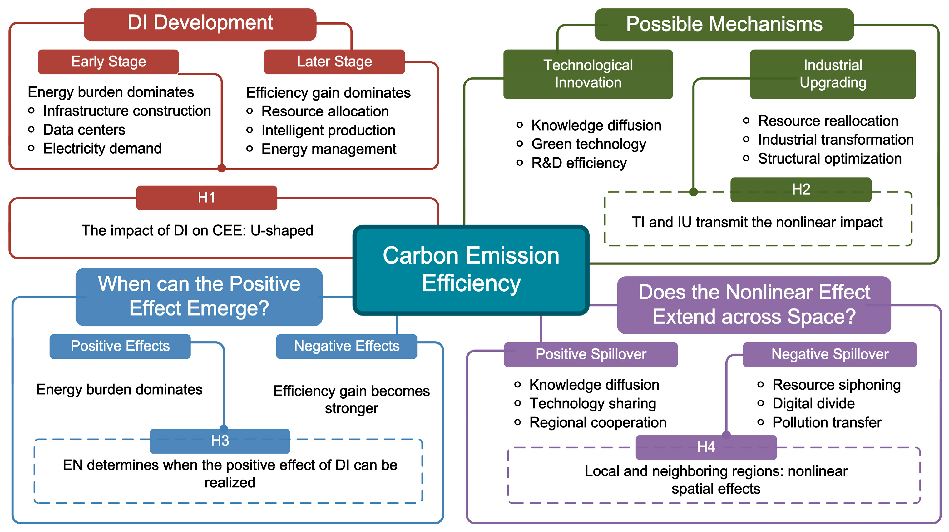
The research framework is presented in Figure 1.

3. Methodology and Data

3.1. Empirical Model

3.1.1. Basic Regression Model

This paper employs a city and year fixed effects model for the baseline regression (Equation (1)). The linear term and the squared term of DI are both included to examine nonlinear effects of DI on CEE.

$$CE{E}_{it}={\beta }_0+{\beta }_{1}D{I}_{it}+{\beta }_{2}D{I}_{it}^2+{\beta }_{k}Contro{l}_{it}+{\mu }_i+{\varphi }_t+{\epsilon }_{it}$$

(1)

In Equation (1), $CE{E}_{it}$ represents the CEE of city $i$ in year $t$. $D{I}_{it}$ represents the development level of DI, and $D{I}_{it}^2$ is the squared term. $Contro{l}_{it}$ is control variables. ${\mu }_i$ and ${\varphi }_t$ denote city and year fixed effects. ${\epsilon }_{it}$ is the random error.

3.1.2. Mediating Effect Model

As discussed in Section 2.2, DI may impact CEE via industrial upgrading and technological innovation. A mediating effect model is therefore employed (Equations (2) and (3)).

$$Me{d}_{it}={\alpha }_0+{\alpha }_{1}D{I}_{it}+{\alpha }_{2}D{I}_{it}^2+\sum _k{\alpha }_{k}Contro{l}_{k,it}+{\mu }_i+{\varphi }_t+{\epsilon }_{it}$$

(2)

$$CE{E}_{it}={\beta }_0+{\beta }_{1}D{I}_{it}+{\beta }_{2}D{I}_{it}^2+{\beta }_{3}Me{d}_{it}+\sum _k{\beta }_{k}Contro{l}_{k,it}+{\mu }_i+{\varphi }_t+{\epsilon }_{it}$$

(3)

In these equations, $Me{d}_{it}$ represents the mediating variables. Definitions of other variables are in line with those in Equation (1).

3.1.3. Threshold Effect Model

Since the construction and operation of DI are characterized by high energy demand, this study adopts energy efficiency as a threshold variable to investigate whether the influence is conditional. A panel threshold model is adopted for empirical estimation, as specified in Equation (4).

$$\begin{array}{l}CE{E}_{it}={\theta }_0+{\theta }_{11}D{I}_{it}\times I\left(Q_{it}\le r\right)+{\theta }_{12}D{I}_{it}\times I\left(Q_{it}>r\right)+{\displaystyle \sum _k}{\theta }_{k}Contro{l}_{k,it}\\ +{\mu }_i+{\varphi }_t+{\epsilon }_{it}\end{array}$$

(4)

In Equation (4), $Q_{it}$ represents the threshold variable, and $r$ denotes the value of the threshold $I(\cdot )$ represents the indicator function, which equals 1 when the condition in parentheses is satisfied and 0 otherwise. Definitions of other variables are in line with those in Equation (1).

3.1.4. Spatial Autocorrelation

Before applying spatial econometric models, spatial autocorrelation is tested. Global spatial dependence is commonly measured using Moran’s I, as reported in Equations (5) and (6).

$$I={\displaystyle \frac{{\sum }_{i=1}^n{\sum }_{j=1}^n{w}_{ij}\left(\right(x_i-\overline{x}\left)\right(x_j-\overline{x}\left)\right)}{S^2{\sum }_{i=1}^n{\sum }_{j=1}^n{w}_{ij}}}$$

(5)

$$S^2={\displaystyle \frac{{\sum }_{i=1}^n(x_i-\overline{x}{)}^2}{n}}$$

(6)

In these equations, $S^2$ denotes the sample variance. $w_{ij}$ is an element of the spatial weight matrix. $x_i$ and $x_j$ represent the values of the variable in city $i$ and $j$, where $i\ne j$. $n$ and $\overline{x}$ are the total number and the average value of the observations.

3.1.5. Spatial Durbin Model

We employ a spatial econometric model to explore the spatial spillover effect of DI on CEE. The appropriate spatial econometric model was determined by using LM, Hausman, Wald and LR tests. The test results indicate that the most suitable model is SDM (Equation (7)).

$$\begin{array}{ll}CE{E}_{it}={\gamma }_0+& \rho {\displaystyle \sum _{j=1}^n}{w}_{ij}CE{E}_{jt}+{\gamma }_{1}D{I}_{it}+{\gamma }_{2}D{I}_{it}^2+{\displaystyle \sum _k}{\gamma }_{k}Contro{l}_{k,it}\\ & \hspace{1em}+{\theta }_1{\displaystyle \sum _{j=1}^n}{w}_{ij}D{I}_{jt}+{\theta }_2{\displaystyle \sum _{j=1}^n}{w}_{ij}D{I}_{jt}^2+{\displaystyle \sum _k}{\theta }_k{\displaystyle \sum _{j=1}^n}{w}_{ij}Contro{l}_{k,jt}\\ & \hspace{1em}+{\mu }_i+{\varphi }_t+{\epsilon }_{it}\end{array}$$

(7)

In Equation (7), $\gamma$ represents the direct effects of DI, $\rho$ denotes the spatial autoregressive coefficient of CEE. and $\theta$ captures their spatial spillover effects.

3.2. Variables and Data

3.2.1. The Dependent Variable: CEE

Compared with single-factor indicators, total factor CEE takes into account both economic output and environmental costs more comprehensively. CEE is estimated using the global super-efficiency Slacks-based Measure (SBM) model.

For city $j$, the input vector is defined as $x_j=(x_{1j},\dots ,x_{mj})\in R_{+}^m$, the desirable output vector as $y_j=(y_{1j},\dots ,y_{s_{1}j})\in R_{+}^{s_1}$ and the undesirable output vector as $b_j=(b_{1j},\dots ,b_{s_{2}j})\in R_{+}^{s_2}$. The global production possibility set constructed across all cities and all periods is given in Equation (8).

$$P^G=\left\{(x,y,b)\left|\sum _{j=1}^n{\lambda }_j{x}_j\le x,\sum _{j=1}^n{\lambda }_j{y}_j\ge y,\sum _{j=1}^n{\lambda }_j{b}_j\le b,{\lambda }_j\ge 0\right.\right\}$$

(8)

For the evaluated city $o$, the global super-efficiency SBM model is defined in Equations (9) and (10).

$$\underset{{\rho }^G,\lambda ,s^{-}.s^y,s^b}{min}{\rho }^G={\displaystyle \frac{1+\frac{1}{m}{\sum }_{i=1}^m\frac{s_i^{-}}{x_{io}}}{1-\frac{1}{s_1+s_2}\left({\sum }_{r=1}^{s_1}\frac{s_r^y}{y_{ro}}+{\sum }_{q=1}^{s_2}\frac{s_q^b}{b_{qo}}\right)}}$$

(9)

$$s.t.\left\{\begin{array}{l}{x}_{io}={\displaystyle \sum _{\begin{array}{c}j=1\\ j\ne o\end{array}}^n}{\lambda }_j{x}_{ij}+s_i^{-},\hspace{1em}i=1,\dots ,m,\\ y_{ro}={\displaystyle \sum _{\begin{array}{c}j=1\\ j\ne o\end{array}}^n}{\lambda }_j{y}_{rj}-s_r^y,\hspace{1em}r=1,\dots ,s_1,\\ b_{qo}={\displaystyle \sum _{\begin{array}{c}j=1\\ j\ne o\end{array}}^n}{\lambda }_j{b}_{qj}+s_q^b,\hspace{1em}q=1,\dots .s_2,\\ {\lambda }_j\ge 0,s_i^{-}\ge 0,s_r^y\ge 0,s_q^b\ge 0.\end{array}\right.$$

(10)

$x_j$, $y_j$, and $b_j$ represent the input, desirable output, and undesirable output vectors of city $j$. ${\lambda }_j$ is the intensity variable. ${\rho }^G$ represents the global super-efficiency score. $x_{io}$, $y_{ro}$, and $b_{qo}$ refer to the i-th input, r-th desirable output, and q-th undesirable output of city $o$. The indicators are reported in

Table 1. Indicators for the super-efficiency SBM model.

Indicator Type	Indicator	Description
Input	Capital	Urban Capital Stock Estimated via the Perpetual Inventory Method
	Labor	Year-end Total Employment
	Energy Consumption	Standard coal equivalent of energy consumption (Natural Gas, Liquefied Petroleum Gas, and Electricity)
Desirable Output	Gross Regional Product	Real GDP
Undesirable Output	Carbon Emission	EDGAR CO2

.

3.2.2. The Independent Variable: DI

DI is calculated using the entropy method.

Table 2. Indicator system of DI.

Dimensions	Indicators
Digital Connectivity	Density of base stations
	Long-distance optical cable density
Digital Service Capacity	Per capita telecommunication business volume
	Internet users per 10,000 people
	Mobile phone subscribers per 10,000 people
Digital Human Capital	Share of employees in the Internet industry

shows the indicator system. Data on long-distance fiber optic cable length are not available at the city level. Provincial cable lengths are therefore allocated to cities according to their share of total telecommunication business [55]. Since the number of base stations exhibits exponential growth, both the number of base stations and administrative area are transformed using natural logarithms to mitigate the influence of extreme values before calculating base station density.

3.2.3. Mechanism Variables

Industrial upgrading (IU) and technological innovation (TI) are the mechanism variables. IU is calculated by the weighted level of IU. The primary, secondary, and tertiary industries are assigned values of 1, 2 and 3, respectively. A weighted sum is then calculated to reflect the overall upgrading level [56]. The number of invention patents obtained per 100 people is used to measure TI.

3.2.4. Threshold Variable

The threshold variable is energy efficiency (EN). It is represented by the ratio of real GDP (10⁴ yuan) to the total energy consumption (ton of standard coal) and reflects the economic output per unit of energy input.

3.2.5. Control Variables

Five control variables are presented as follows: financial development (FI), population density (PO), economic density (EC), openness to trade (OP), and education development (ED). FI is measured as the ratio of deposits of financial institutions to GDP. PO is defined as the resident population per km². EC is measured as GDP to the administrative area of the city. OP is indicated by the logarithm of total import and export volume. ED is represented by the ratio of college students to the resident population.

3.2.6. Data Source

The global gridded carbon emission data are obtained from EDGAR. City-level carbon emissions are derived using spatial analysis tools in ArcGIS 10.7. Standard coal conversion coefficients for three energy types are taken from the China Energy Statistical Yearbook. Other data are collected from the China Urban Construction Statistical Yearbook, the China City Statistical Yearbook, and local statistical yearbooks. A few unpublished missing data were filled in by linear interpolation. The descriptive statistics are presented in

Table 3. Descriptive statistics.

Variable	Obs	Mean	SD	Min	Median	Max
CEE	574	0.508	0.177	0.200	0.478	1.738
DI	574	0.221	0.135	0.027	0.194	0.880
IU	574	2.388	0.123	2.052	2.393	2.780
TI	574	0.040	0.047	0.000	0.024	0.327
EN	574	8.773	2.098	4.584	8.454	16.504
FI	574	1.564	0.578	0.198	1.494	4.100
PO	574	0.075	0.060	0.012	0.063	0.393
EC	574	17.278	0.972	15.147	17.253	20.106
OP	574	6.364	1.765	2.566	6.399	10.663
ED	574	0.199	0.169	0.022	0.161	1.101

.

4. Empirical Results and Discussion

4.1. Benchmark Regression

Columns (1) and (2) in

Table 4. Results of benchmark regression.

Variables	(1)	(2)	(3)	(4)
	CEE	CEE	CEE	CEE
DI	0.483 ***	0.366 ***	−1.527 ***	−1.612 ***
	(4.62)	(3.60)	(−7.93)	(−7.33)
DI2			1.887 ***	1.904 ***
			(10.87)	(9.35)
FI		−0.029		−0.056 ***
		(−1.49)		(−3.60)
PO		1.819 ***		0.918 ***
		(4.96)		(3.08)
EC		0.239 ***		0.307 ***
		(3.66)		(5.08)
OP		−0.064 ***		−0.036 ***
		(−4.52)		(−2.77)
ED		0.213 *		0.213 **
		(1.67)		(2.00)
Constant	0.401 ***	−3.425 ***	0.719 ***	−4.371 ***
	(17.00)	(−3.06)	(22.01)	(−4.24)
N	574	574	574	574
R2	0.780	0.801	0.812	0.829
Adj. R2	0.76	0.78	0.79	0.81
City FE	Yes	Yes	Yes	Yes
Year FE	Yes	Yes	Yes	Yes

Note: The value of t is in parentheses.; *, **, and *** are significant at the level of 10%, 5%, and 1%, respectively.

present the linear specification. With or without control variables, the coefficient of DI is significant and positive. This indicates that DI can improve CEE.

To examine possible nonlinear effects, a squared term of DI is included (Columns (3) and (4)). The coefficient of DI is significantly negative, while the coefficient of DI² is significantly positive. The value of R² increases after the squared term is added, which means improved explanatory power. These results indicate a U-shaped influence of DI on CEE. Coefficients are not sufficient to confirm the nonlinear influence, and a U-shaped relationship test is required (

Table A1. U-shaped relationship test.

	Lower Bound	Upper Bound
Interval	0.027	0.880
Slope	−1.508	1.739
t-value	−7.194	10.236
p > |t|	0.000	0.000

in Appendix A.1). The result is significant at the 1% level, and the turning point is 0.423. It lies within the range of DI. In 2024, only Shanghai, Nanjing, Wuxi, Suzhou, Hangzhou, Ningbo and Hefei had a DI level higher than this threshold. Among them, Shanghai, Nanjing, Hangzhou and Hefei are provincial capitals or municipalities. Most cities remain below the turning point, which implies that the promoting influence of DI on CEE has not emerged in many cities.

4.2. Robustness and Endogeneity Tests

4.2.1. Robustness Tests

The robustness tests are shown in

Table 5. Results of robustness tests.

Variables	(1)	(2)	(3)	(4)	(5)
	CEE	CEE	CEE	CEE	CEE
DI	−1.897 ***	−1.657 ***	−1.304 ***	−1.548 ***	−1.878 ***
	(−9.01)	(−7.62)	(−6.16)	(−7.62)	(−5.42)
DI2	2.295 ***	2.055 ***	1.649 ***	1.860 ***	2.398 ***
	(11.95)	(10.02)	(8.05)	(9.77)	(4.97)
FI	−0.058 ***	−0.059 ***	−0.054 ***	−0.051 ***	−0.060 ***
	(−4.21)	(−3.55)	(−3.38)	(−3.70)	(−3.42)
PO	0.820 ***	1.085 ***	1.302 ***	0.981 ***	0.761 **
	(2.82)	(3.97)	(4.02)	(3.34)	(2.58)
EC	0.280 ***	0.291 ***	0.285 ***	0.299 ***	0.331 ***
	(5.30)	(4.28)	(4.58)	(5.20)	(5.01)
OP	−0.033 **	−0.037 ***	−0.043 ***	−0.037 ***	−0.029 **
	(−2.57)	(−2.59)	(−3.27)	(−3.02)	(−2.14)
ED	0.243 **	0.265 **	0.204 *	0.198 **	0.331 ***
	(2.42)	(2.49)	(1.88)	(1.97)	(2.67)
Constant	−3.868 ***	−4.101 ***	−4.039 ***	−4.248 ***	−4.750 ***
	(−4.33)	(−3.51)	(−3.81)	(−4.33)	(−4.25)
N	574	533	574	574	518
R2	0.873	0.832	0.824	0.874	0.803
Adj. R2	0.86	0.81	0.80	0.86	0.78
City FE	Yes	Yes	Yes	Yes	Yes
Year FE	Yes	Yes	Yes	Yes	Yes

Note: The value of t is in parentheses. *, **, and *** are significant at the level of 10%, 5%, and 1%, respectively.

. Column (1) presents the regression results after winsorizing all variables at 1% level to reduce the impact of extreme values. In column (2), the independent variable is lagged by one period to investigate its lag effect, because the change in CEE requires a certain period. Column (3) remeasures DI using the entropy-TOPSIS method. Column (4) uses the global SBM model instead of the super-efficiency SBM model to calculate CEE. In Column (5), since municipalities directly under the central government and provincial capitals have significant advantages in terms of politics, population, and economy, these cities were excluded from the regression analysis. In Table 5, all the coefficients of DI remain negative, and the squared term remains positive. The estimated relationship and significance levels are in line with the baseline regression.

4.2.2. Endogeneity Tests

To address the possible two-way causality between DI and carbon emission efficiency, as well as omitted variable bias, this study employs the two-stage least squares (2SLS) method for estimation (

Table 6. Results of endogeneity tests.

Variables	Stage One		Stage Two
	(1)	(2)	(3)
	DI	DI2	CEE
IV1	−0.355 ***	−0.359 ***
	(−4.61)	(−3.93)
IV2	0.103 ***	0.178 ***
	(3.32)	(4.78)
DI			−5.337 ***
			(−3.71)
DI2			6.456 ***
			(5.41)
FI	0.028 *	0.039 **	−0.143 ***
	(1.77)	(2.00)	(−3.57)
PO	0.436	0.822 **	−1.716 *
	(1.64)	(2.49)	(−1.78)
EC	0.029	−0.007	0.430 ***
	(0.98)	(−0.22)	(4.89)
OP	−0.010	−0.020 **	0.054 **
	(−1.35)	(−2.46)	(2.05)
ED	0.155	0.163	0.050
	(1.41)	(1.17)	(0.17)
Constant	−0.328	0.155	−6.504 ***
	(−0.64)	(0.28)	(−4.54)
N	574	574	574
R2	0.932	0.851	0.625
Adj. R2	0.92	0.83	0.58
Under-identification Test	16.600 ***
Weak Identification Test	10.088
10% Maximal IV Size	7.03

Note: The value of t is in parentheses. *, **, and *** are significant at the level of 10%, 5%, and 1%, respectively.

). Based on the studies of Nunn and Qian (2014) [57], Huang et al. (2019) [58], and Liu and Ma (2020) [59], we select two instrumental variables. The first is the interaction term between the average terrain relief and a time trend (IV1). The second is the interaction term between the number of post offices in 1984 and a time trend (IV2). The average terrain relief reflects the geographical limitations of infrastructure construction, while the historical postal infrastructure reflects the early foundation of the communication network. Although geographical conditions and historical infrastructure may be related to the long-term development of the region, by incorporating city fixed effects, year fixed effects, and control variables, the potential impact of these factors on current CEE is mitigated.

In terms of the empirical results, the first-stage regression shows that both of the two instrumental variables are significantly correlated with DI and DI², indicating sufficient relevance. Further identification tests reveal that the under-identification test statistic is 16.600, which rejects the null hypothesis of under-identification at the 1% level. This suggests that the instrumental variables can effectively explain the variation in the endogenous variables. The weak instrumental variable test statistic is 10.088, indicating that the strength of the instrumental variables is within the acceptable range. In the second-stage results, the coefficient of the linear term of DI is significantly negative, while the coefficient of the squared term is significantly positive. This implies that the impact of DI on CEE follows a U-shaped pattern. The results are consistent with the findings of the baseline regression.

4.3. Mechanism Analysis

As discussed in Section 2.2, TI and IU may help explain the nonlinear impact of DI on CEE. This section examines these potential channels (

Table 7. Results of mechanism analysis.

Variables	(1)	(2)	(3)	(4)	(5)	(6)
	CEE	TI	CEE	IU	CEE	CEE
DI	−1.612 ***	−0.368 ***	−1.368 ***	0.538 ***	−1.368 ***
	(−7.33)	(−5.36)	(−5.82)	(4.70)	(−6.57)
DI2	1.904 ***	0.581 ***	1.519 ***	−0.454 ***	1.698 ***
	(9.35)	(9.14)	(6.38)	(−4.23)	(9.06)
FI	−0.056 ***	−0.010 **	−0.050 ***	0.015	−0.050 ***	−0.025
	(−3.60)	(−1.98)	(−3.24)	(1.41)	(−3.25)	(−1.15)
PO	0.918 ***	0.288 ***	0.727 **	−0.480 ***	0.700 **	1.317 ***
	(3.08)	(2.92)	(2.47)	(−2.86)	(2.33)	(3.75)
EC	0.307 ***	−0.010	0.314 ***	0.095 ***	0.351 ***	0.353 ***
	(5.08)	(−0.70)	(5.26)	(2.96)	(5.94)	(5.46)
OP	−0.036 ***	−0.009 ***	−0.030 **	0.031 ***	−0.022 *	−0.044 ***
	(−2.77)	(−2.68)	(−2.38)	(4.18)	(−1.67)	(−2.97)
ED	0.213 **	0.140 ***	0.120	−0.179 ***	0.131	0.159
	(2.00)	(4.16)	(1.05)	(−3.21)	(1.32)	(1.34)
TI			0.663 ***
			(3.02)
IU					−0.454 ***	−4.212 ***
					(−4.73)	(−3.82)
IU2						0.791 ***
						(3.33)
Constant	−4.371 ***	0.283	−4.558 ***	0.508	−4.140 ***	0.139
	(−4.24)	(1.11)	(−4.51)	(0.93)	(−4.11)	(0.08)
N	574	574	574	574	574	574
R2	0.829	0.870	0.833	0.938	0.836	0.811
Adj. R2	0.81	0.85	0.81	0.93	0.82	0.79
City FE	Yes	Yes	Yes	Yes	Yes	Yes
Year FE	Yes	Yes	Yes	Yes	Yes	Yes

Note: The value of t is in parentheses. *, **, and *** are significant at the level of 10%, 5%, and 1%, respectively.

). The bootstrap test results are reported in Appendix A.2.

Columns (2) and (3) examine the potential role of TI. Column (2) shows that the impact of DI on TI is U-shaped. In the early stage of digital development, investment tends to focus on the deployment of DI rather than the advancement of digital technologies. The expansion of DI requires funds, organizational adaptation, and technological learning, which may temporarily constrain innovation activities. As DI becomes more developed, it may provide stronger support for knowledge diffusion, information sharing, and innovation activities. Column (3) shows that TI has a positive effect on CEE. These results suggest that TI may be an important channel through which DI influences CEE, especially in the later stage of development.

Columns (4) and (5) examine the potential role of IU. Column (4) shows that the impact of DI on IU is inverted U-shaped. DI may initially promote the transformation of traditional industries by improving information flow and reducing transaction costs. However, when the development of DI reaches a relatively high level, the marginal effect of DI on IU may become weaker. This does not necessarily mean that DI inhibits the industrial transformation. One possible explanation is that the IU indicator used in this study is constructed based on the weighted shares of the three industries. In the later stage of development, IU may increasingly be achieved through manufacturing servitization and improvements in production quality, rather than continuous changes in the composition of the three industries. Such changes may maintain or even increase the share of the secondary sector, thereby reducing the measured level of IU.

Column (5) shows that the linear impact of IU on CEE is negative. When the squared term of IU is considered in Column (6), the impact of IU on CEE is U-shaped. This suggests that the environmental benefits of IU may not appear immediately. In the early stage, traditional and emerging industries may coexist. This stage involves adjustment costs, reallocating capital, and expanding new production capacity. These processes may temporarily increase energy demand and reduce CEE. In the later stage, the benefits of IU, such as higher value-added production and improved resource allocation, may become more evident. Therefore, the negative effect of IU on CEE may indicate that many cities are still in the process of adjustment. The transformation costs have not been fully covered by efficiency gains.

Overall, the mechanism analysis suggests that IU and TI may be associated with different stages. The mechanism analysis provides a possible explanation for the nonlinear impact of DI on CEE rather than definitive evidence of causal mechanisms. IU seems to be more closely related to the adjustment stage. In this stage, the transformation costs may weaken CEE. When digital capabilities become mature and efficiency gains increase, TI may play a more significant role. These findings suggest that the nonlinear impact may result from changes in the relative contribution of different paths.

4.4. Threshold Effect Analysis

This study employs energy efficiency (EN) as the threshold variable. EN is measured as the ratio of real GDP to total energy consumption. It represents the economic output generated per unit of energy input.

Table 8. Threshold effect test.

Threshold	F-Value	p-Value	The Critical Value
			1%	5%	10%
Single	44.24	0.0133	46.6694	37.0094	29.6998
Double	19.33	0.2900	45.8258	34.8334	28.0461

supports the existence of a single threshold.

Table 9. Threshold regression.

Variables	(1)
	CEE
FI	−0.028
	(−1.29)
PO	1.781 ***
	(4.05)
EC	0.303 ***
	(4.28)
OP	−0.046 ***
	(−3.05)
ED	0.226 *
	(1.75)
DI (EN ≤ 8.533)	0.066
	(0.63)
DI (EN > 8.533)	0.369 ***
	(4.01)
Constant	−4.571 ***
	(−3.90)
N	574
R2	0.606
Adj. R2	0.56
City FE	Yes
Year FE	Yes

Note: The value of t is in parentheses. *, and *** are significant at the level of 10% and 1%, respectively.

presents the results of the threshold regression model. The estimated threshold value of EN is 8.533 (10⁴ yuan/ton of standard coal). It should be noted that this threshold value is estimated based on the settings of this study. The threshold value may vary across different study regions, study periods, and measurement methods. Therefore, the value of 8.533 should not be interpreted as a universal global benchmark. In this study, when energy efficiency (EN) is below 8.533, the impact of DI is positive but insignificant. This indicates that the environmental benefits of DI have not been realized. When energy efficiency (EN) exceeds 8.533, DI shows a positive impact on CEE.

The results indicate that EN determines when the environmental benefits of DI can emerge. In regions with lower EN, the same computing and production tasks require more energy consumption. Inefficient energy use may cause additional energy demands. Under such conditions, the positive impact on CEE is insufficient to reach statistical significance. When EN exceeds the threshold value, the energy costs of digital operations become lower. The role of DI in improving production efficiency, optimizing resource allocation, and strengthening energy management can be better realized. Therefore, EN is an important factor for enabling DI to achieve significant environmental benefits.

4.5. Spatial Effects of DI on CEE

4.5.1. Spatial Correlation Test

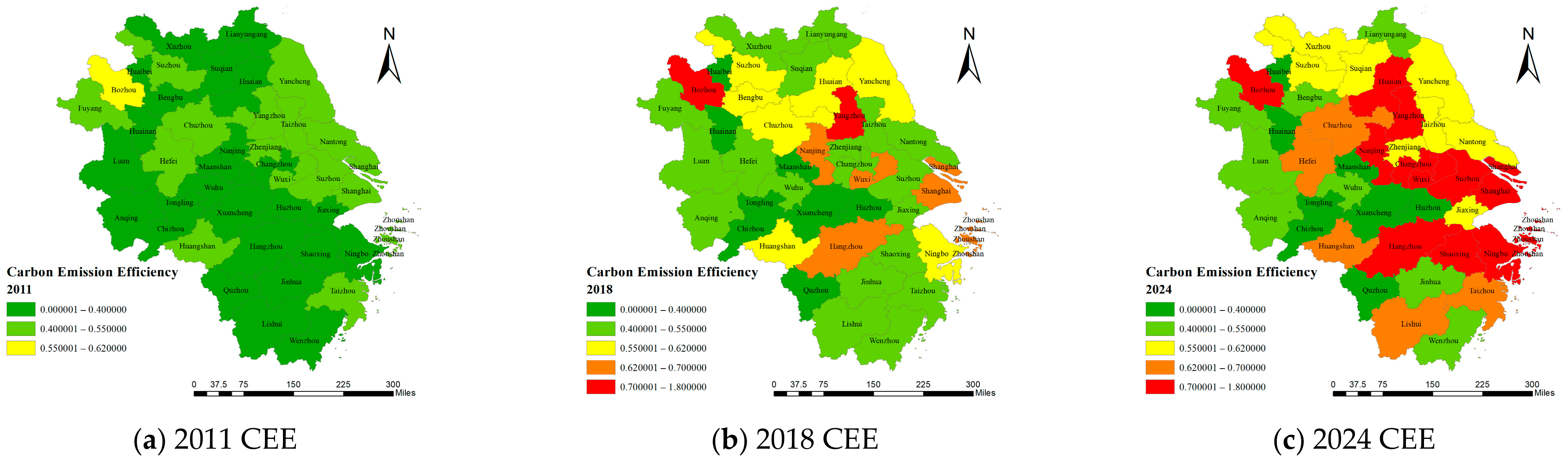
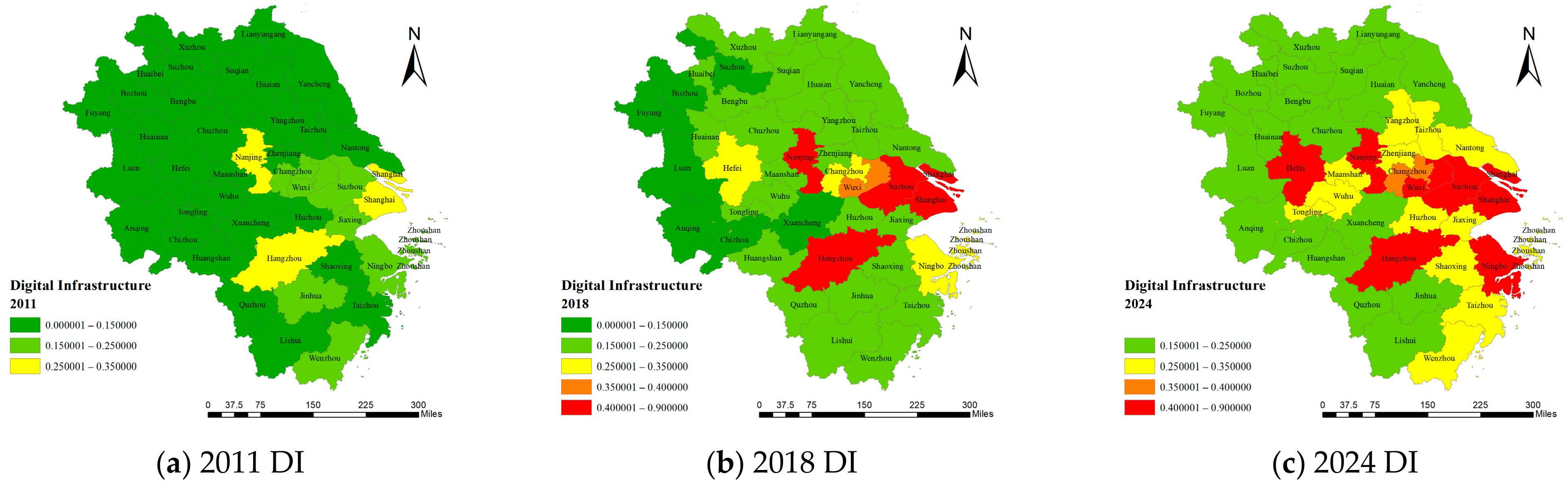
To visualize the spatial distribution and the evolution, data from 2011, 2018 and 2024 were plotted using ArcGIS 10.7 (Figure 2 and Figure 3). The overall level of DI has been improving over time. The areas with high values are concentrated in Shanghai, the southern part of Jiangsu Province, and the northern part of Zhejiang Province, and they gradually spread from the well-developed cities to the surrounding regions. In the early stage, the spatial distribution of cities with high CEE is relatively scattered. Over time, high value areas become more concentrated in cities with stronger economic foundations, and the spatial patterns of DI and CEE show a similar distribution. These results indicate that this study is suitable for using spatial econometric models.

Moran’s I based on the geographical distance matrix is employed in this study to examine the spatial correlation.

Table A3. Results of Moran’s I test.

Year	DI			CEE
	Moran’s I	Z-Statistic	p-Value	Moran’s I	Z-Statistic	p-Value
2011	0.651	7.717	0.000	0.113	1.590	0.112
2012	0.631	7.541	0.000	0.122	1.673	0.094
2013	0.534	6.810	0.000	0.100	1.430	0.153
2014	0.528	6.602	0.000	0.081	1.244	0.213
2015	0.542	6.756	0.000	0.099	1.627	0.104
2016	0.550	6.847	0.000	0.173	2.252	0.024
2017	0.583	7.287	0.000	0.127	1.742	0.082
2018	0.515	6.732	0.000	0.194	2.488	0.013
2019	0.526	6.768	0.000	0.139	1.893	0.058
2020	0.697	8.684	0.000	0.172	2.256	0.024
2021	0.693	8.640	0.000	0.242	3.048	0.002
2022	0.534	6.842	0.000	0.302	3.696	0.000
2023	0.545	6.998	0.000	0.311	3.787	0.000
2024	0.562	7.199	0.000	0.247	3.237	0.001

in Appendix A.3 shows that Moran’s I is significant and positive in most years, which partly supports the existence of spatial dependence.

4.5.2. Spatial Effect Analysis

The SDM model with two-way fixed effects is adopted according to the results of the LM, LR, Wald and Hausman tests (

Table A4. Identification tests for the spatial econometric model.

Tests	Statistic	p-Value
Hausman	334.05 ***	0.000
LM-lag	39.376 ***	0.000
Robust–LM-lag	53.179 ***	0.000
LM-error	11.266 ***	0.001
Robust–LM-error	25.069 ***	0.000
LR-SDM/SAR	42.94 ***	0.000
LR-SDM-SEM	53.58 ***	0.000
Wald-SAR	43.46 ***	0.000
Wald-SEM	54.11 ***	0.000

Note: *** indicates significance at the 1% level.

in Appendix A.4). This analysis employs a geographical distance matrix. To ensure the robustness of the spatial effect estimation, a series of additional tests are conducted, including using different spatial weight matrices and re-measuring key variables. The results can be found in Appendix A.5.

Table 10. Results of spatial effect analysis.

Variables	(1)	(2)	(3)	(4)	(5)
	Main	Wx	Direct	Indirect	Total
DI	−1.179 ***	−1.391 ***	−1.216 ***	−1.835 ***	−3.051 ***
	(0.216)	(0.524)	(0.221)	(0.548)	(0.583)
DI2	1.372 ***	1.168 **	1.401 ***	1.625 ***	3.027 ***
	(0.207)	(0.473)	(0.211)	(0.472)	(0.490)
FI	−0.045 **	0.247 ***	−0.036 **	0.278 ***	0.242 ***
	(0.019)	(0.065)	(0.018)	(0.077)	(0.079)
PO	0.605	2.239 **	0.669 *	2.648 **	3.317 ***
	(0.397)	(0.906)	(0.384)	(1.039)	(1.134)
EC	0.284 ***	−0.265	0.279 ***	−0.242	0.037
	(0.062)	(0.171)	(0.059)	(0.210)	(0.218)
OP	−0.024 *	−0.004	−0.024 *	−0.011	−0.035
	(0.014)	(0.031)	(0.014)	(0.035)	(0.036)
ED	0.266 **	1.212 ***	0.304 **	1.461 ***	1.766 ***
	(0.114)	(0.280)	(0.122)	(0.345)	(0.405)
Spatial rho	0.159 **	sigma2_e	0.005 ***	N	574
	(0.074)		(0.000)	R-squared	0.086
City FE	Yes	Yes	Yes	Yes	Yes
Year FE	Yes	Yes	Yes	Yes	Yes

Note: The value of t is in parentheses. *, **, and *** are significant at the level of 10%, 5%, and 1%, respectively.

shows that the local and spatial spillover effects of DI display a negative linear term and a positive squared term, suggesting a potential U-shaped impact on CEE. However, the signs and significance of the coefficients of DI and DI² are not sufficient to confirm the existence of a U-shaped impact. We further conducted the nonlinear effect verification. The results are reported in Appendix A.6. Based on the results in Table 10 and

Table A6. Nonlinear effect verification of the SDM model.

City Type	DImin	DImax	Effect	Turning Point	ME (DImin)	ME (DImax)	Pattern
All	0.027	0.880	Direct	0.434	−1.140	1.250	U
			Indirect	0.565	−1.747	1.025	U
Non-Resource-based Cities	0.027	0.880	Direct	0.410	−1.270	1.557	U
			Indirect	0.577	−5.467	3.016	U
Resource-based Cities	0.031	0.296	Direct	0.129	1.105	−1.869	Inverted-U
			Indirect	0.089	1.745	−6.190	Inverted-U
Low Carbon Pilot Cities	0.027	0.880	Direct	0.444	−1.939	2.029	U
			Indirect	0.413	−3.132	3.789	U
Non-pilot Cities	0.031	0.465	Direct	0.312	−1.421	0.773	U
			Indirect	-	-	-	Linear effect
High Per Capita GDP	0.067	0.880	Direct	0.447	−1.356	1.543	U
			Indirect	0.656	−4.226	1.606	U
Low Per Capita GDP	0.027	0.275	Direct	0.211	−1.052	0.369	U
			Indirect	0.116	1.611	−2.904	Inverted-U

, the direct effect and spatial spillover effect of DI on CEE are U-shaped.

For local effects, the early stage of DI development involves large-scale investment and rising energy demand. The building of data centers, the expansion of communication networks, and the operation of computing equipment all rely heavily on electricity. Before the improvement in efficiency is evident, energy consumption is likely to increase. In this stage, the impact of technology and productivity has not been fully realized [33,60], which may limit the improvement of CEE. With the maturation of DI, economies of scale and network externalities gradually emerge. By promoting industrial digital transformation, improving energy management, enhancing productivity, and encouraging the clustering of high-value industries, digital technologies begin to enhance energy efficiency and optimize the reallocation of resources, thereby significantly improving CEE and achieving a transformation from suppression to promotion.

For the spillover effect, during the initial stage, the core cities may attract capital, technology and skilled labor from the surrounding areas [45]. This will exacerbate regional imbalances, leading to the outflow of resources and the hollowing out of industries in surrounding areas. Some industries with high energy consumption or low added value may relocate within the region, resulting in a temporary “pollution transfer” or factor displacement effect [61]. These factors will temporarily reduce CEE in the surrounding areas. Over time, with the expansion of DI, the mechanisms for information sharing, technology diffusion and collaborative innovation among regions are strengthened. Digital technology spreads across space through learning and demonstration effects [48], promoting the upgrading of industries and the adoption of green technologies in surrounding areas. Furthermore, the interconnection achieved through digital platforms and intelligent networks has reduced trade costs, enhanced coordination, and improved resource allocation [62]. Industrial upgrading and the adoption of green technologies are more likely to occur in nearby cities. Meanwhile, digital platforms and intelligent networks can reduce transaction costs and enhance coordination efficiency and resource allocation [63]. These processes are related to improvements of CEE in surrounding regions.

4.6. Heterogeneity Analysis

Although the benchmark regression model can be used to examine the heterogeneity effects, this method can only capture the differences in local effects and may lead to an incomplete understanding of heterogeneity. Given that both DI and CEE exhibit spatial dependence, and the results of the SDM model confirm the existence of spatial spillover effects, this study adopts a spatial econometric model for heterogeneity analysis. Specifically, cities are classified based on their resource endowment (12 resource-based cities and 29 non-resource-based cities), policy environment (18 low-carbon pilot cities and 23 non-pilot cities), and economic development level (21 high per capita GDP cities and 20 low per capita GDP cities). The classification of resource-based cities is based on the National Sustainable Development Plan for Resource-based Cities (2013–2020) issued by China’s State Council. The classification of low-carbon pilot cities is based on the three batches of national low-carbon city pilots launched by China’s National Development and Reform Commission (NDRC) in 2010, 2012, and 2017. The 50th percentile of average per capita GDP over the sample period is used as the cutoff for classifying cities into high and low economic development groups. These factors may influence the transition from energy burden to efficiency gain. The results are presented in

Table 11. Results of heterogeneity analysis.

Variable		(1)	(2)	(3)	(4)	(5)	(6)
		Non-Resource-Based Cities	Resource-Based Cities	Low Carbon Pilot Cities	Non-Pilot Cities	High per Capita GDP	Low per Capita GDP
DI	Main	−1.495 ***	1.658 ***	−2.454 ***	−1.751 ***	−1.923 ***	−0.928 ***
		(0.272)	(0.565)	(0.410)	(0.370)	(0.356)	(0.332)
	Wx	−8.589 ***	5.002 *	−9.762 ***	−8.715 ***	−10.020 ***	3.138 *
		(2.442)	(2.590)	(3.119)	(2.473)	(2.943)	(1.832)
	Direct	−1.359 ***	1.453 ***	−2.065 ***	−1.578 ***	−1.595 ***	−1.207 ***
		(0.278)	(0.533)	(0.376)	(0.385)	(0.339)	(0.421)
	Indirect	−5.736 ***	2.673 *	−3.351 **	−5.922 ***	−4.707 ***	2.103 **
		(1.819)	(1.608)	(1.372)	(1.735)	(1.522)	(0.925)
	Total	−7.095 ***	4.125 **	−5.415 ***	−7.499 ***	−6.302 ***	0.896
		(1.861)	(1.771)	(1.473)	(1.804)	(1.602)	(0.687)
DI2	Main	1.780 ***	−6.796 ***	2.800 ***	2.632 ***	2.041 ***	1.659
		(0.251)	(1.437)	(0.390)	(0.640)	(0.341)	(1.077)
	Wx	7.610 ***	−26.406 ***	11.579 ***	4.119	8.116 ***	−17.082 ***
		(2.551)	(6.878)	(2.938)	(4.043)	(3.040)	(5.745)
	Direct	1.657 ***	−5.611 ***	2.326 ***	2.528 ***	1.783 ***	2.865 **
		(0.250)	(1.299)	(0.339)	(0.660)	(0.310)	(1.331)
	Indirect	4.973 ***	−14.971 ***	4.057 ***	2.352	3.587 **	−9.103 ***
		(1.800)	(4.285)	(1.278)	(2.780)	(1.542)	(2.971)
	Total	6.630 ***	−20.582 ***	6.382 ***	4.880 *	5.369 ***	−6.238 ***
		(1.863)	(4.648)	(1.419)	(2.827)	(1.645)	(2.270)
Control Variables		Yes	Yes	Yes	Yes	Yes	Yes
Spatial rho		−0.439 *	−0.613 ***	−1.254 ***	−0.401 *	−0.905 ***	−1.398 ***
		(0.240)	(0.233)	(0.310)	(0.226)	(0.281)	(0.227)
sigma2_e		0.006 ***	0.001 ***	0.005 ***	0.003 ***	0.006 ***	0.001 ***
		(0.000)	(0.000)	(0.000)	(0.000)	(0.001)	(0.000)
N		406	168	252	322	294	280
R2		0.026	0.049	0.001	0.193	0.117	0.053
City FE		Yes	Yes	Yes	Yes	Yes	Yes
Year FE		Yes	Yes	Yes	Yes	Yes	Yes

Note: The value of t is in parentheses. *, **, and *** are significant at the level of 10%, 5%, and 1%, respectively.

. The U-shaped or inverted U-shaped impacts identified in each subgroup are further verified in Appendix A.6.

(1) Resource-based and non-resource-based cities

In non-resource-based cities, the impact of DI on CEE of the local area and its neighboring regions follows a U-shaped pattern. In the early stage, the construction and operation of DI require additional electricity consumption, while the integration of digital technologies with local production systems may still be limited. Therefore, the efficiency gains from digitalization may not immediately offset the additional energy burden. As digital technologies integrate more deeply with industrial activities, they can improve resource allocation, optimize production processes, and support energy management. This may lead to improvements in CEE. The spatial effect of non-resource-based cities is also U-shaped. A possible explanation is that these cities are often more involved in regional industrial networks. In the early stage of DI development, due to differences in environmental regulations and production costs, they may undertake some energy-intensive production activities that were transferred from surrounding areas. The insufficient coordination of DI development may lead to inefficient investment among neighboring regions. However, with the improvement of regional digital connectivity, digital technologies may facilitate information sharing, green technology diffusion, and coordinated environmental management. At this point, the surrounding areas can benefit from digitalization.

In resource-based cities, the impact of DI on the local area and neighboring cities follows an inverted U-shaped pattern. The initial improvement of CEE may be related to the characteristics of resource-based industries. Digital technologies can assist resource enterprises in improving production monitoring, optimizing energy use, and reducing information asymmetry, thereby improving CEE. However, the long-term effect may weaken, as resource-based cities usually face stronger industrial path dependence and are heavily reliant on energy-intensive sectors. As DI expands, energy consumption and the rebound effect resulting from the improved production efficiency may partially offset the environmental benefits. Meanwhile, possible industrial structure adjustment and spatial relocation effects may transfer environmental pressure to neighboring resource-based cities, resulting in a negative spatial spillover effect.

(2) Low-carbon pilot and non-pilot cities

In the low-carbon pilot cities, the impact of DI on CEE of the local area and its neighboring regions follows a U-shaped pattern. The initial negative effect may be related to the costs of digital and low-carbon transformation. Although the pilot cities have stronger policy support for green development, the construction of DI itself requires energy input. Moreover, the digital transformation of existing industries usually involves equipment replacement and system adjustments. This process may increase energy consumption. In the later stage, the combination of digitalization and low-carbon policies may improve CEE. Digital monitoring systems, intelligent energy management, and improved environmental governance can help reduce energy waste and improve emission control. The positive spatial effect may result from policy learning and technology diffusion. Low-carbon pilot cities may share their experiences with neighboring areas, thereby promoting low-carbon development.

For non-pilot cities, DI shows a U-shaped effect on local CEE, but its spatial spillover effect is negative. Without low-carbon policy constraints, DI development may initially focus more on economic expansion and production efficiency rather than on emission reduction. As digital integration deepens, local industries can achieve energy conservation and efficiency improvements. The spatial effect suggests that DI development in non-pilot cities may have a negative impact on neighboring regions. One possible explanation is that these cities may lack effective mechanisms for coordinating low-carbon development. Energy-intensive production activities may be transferred to neighboring regions.

(3) Cities with different levels of economic development

In more economically developed cities, the impact of DI on CEE of the local area and the neighboring regions follows a U-shaped pattern. In the early stage, although economically developed cities usually have stronger digitalization and innovation capacities, the construction and operation of DI still require considerable energy. The transformation of industries involves adjustment costs. This may temporarily reduce CEE. In the later stage, developed cities are equipped to convert digital investments into environmental benefits. Financial resources and technological capabilities can help digitalization to integrate into energy management and green innovation. The positive spatial spillover effect may reflect the stronger radiation capacity of developed cities. Through technology diffusion, industrial connections, and regional cooperation, DI in economically developed cities may benefit neighboring regions.

In economically less developed cities, DI shows a U-shaped effect on local CEE. In the early stage, DI may create energy pressure. As digitalization progresses, digital technologies can help these cities improve production efficiency and reduce resource waste. Interestingly, the spatial spillover effect is inverted U-shaped. The early positive spillover effect may be caused by the improvement of regional connectivity. DI development can strengthen information exchange and facilitate the spread of technology to neighboring regions. In the later stage, the spillover effect becomes negative. A possible explanation is that less-developed cities may compete for resources and industries. Some energy-intensive or low-value-added activities may move to neighboring regions with weaker development capacity. This reduces CEE in neighboring regions.

Overall, the heterogeneity results indicate that the environmental impact of DI is influenced by economic structure, policy environment, and development capacities. Cities with stronger transformation capacity are more likely to move from the energy burden stage to the efficiency improvement stage.

4.7. Discussion

(1) Rethinking the Environmental Role of DI in the AI Era

In the era of AI, the rapid development of cloud computing, large-scale data centers, and generative AI has increased the computing demands and power consumption. This trend has created new environmental challenges. Some studies have focused on whether digitalization improves or harms the environment. This question may not be sufficient in the AI era. DI can bring both energy pressure and new opportunities for efficiency improvement. Therefore, a more important question is whether DI can shift from an energy burden to an efficiency gain.

This study suggests that the environmental impact of DI may change during the development process. One possible explanation is that the energy consumption caused by infrastructure deployment and digital activities occurs immediately, but the efficiency gains do not occur immediately. As digital technologies become integrated into the production systems and management processes, the efficiency improvements may gradually emerge. Whether DI has a net positive impact on CEE depends on whether the efficiency gains that support low-carbon development can offset the energy burden. Therefore, the construction of DI should not only consider its short-term costs but also recognize its potential to improve resource allocation and production efficiency in the long run. The “from energy burden to efficiency gain” perspective of this study shifts the focus from “whether digitalization is green” to “how digitalization can become green”. This transition is important in the AI era.

(2) Broader Relevance Beyond the YRD Region

The issue of energy consumption from DI is not unique to the YRD region. Many countries and regions are facing similar challenges in the AI era. For example, in the United States, the expansion of AI and data centers has put pressure on electricity demand. The U.S. Energy Information Administration (EIA) [64] reports that the energy consumption of data center servers is becoming a major driver of electricity demand. By 2050, the electricity consumption of data center servers alone is projected to reach 446–818 billion kWh [64]. Japan provides another example of DI expansion. The geographical distribution of data centers in Japan is highly uneven. Data centers are concentrated in the Tokyo metropolitan area, and the new power supply applications for these data centers far exceed the grid capacity. To address this challenge, Japan implemented the “Watt-Bit Collaboration”. The Japanese case shows that the operation of digital activities requires the support of energy systems. Similar to the grid capacity challenges in the Tokyo metropolitan area, in some European regions, there is also a mismatch between DI expansion and the power systems. The distribution of renewable energy resources in Europe is uneven. Offshore wind resources are concentrated in the North Sea region. Solar energy resources are more abundant in Southern Europe. However, digital activities in Europe are concentrated in major data center hubs such as Frankfurt, London and Dublin. The increasing electricity demands put more pressure on the environment.

The YRD region provides an appropriate case for studying the impact of DI on low-carbon development. First, the region contains cities at different digital development stages. Some cities have already established mature digital ecosystems, while others are still expanding DI and related industries. This allows us to explore whether the environmental impact of DI changes at different stages. This is related to the “from energy burden to efficiency gain” perspective of this study. Second, the cities in the YRD region have close ties with each other. The YRD region implements an integrated development strategy. It is characterized by close economic ties and interconnected digital networks. These features create conditions for technology diffusion, information sharing, and regional cooperation, making the region suitable for exploring the spatial spillover effects of DI.

It should be noted that the experience of the YRD region may not be directly applicable to all regions. The YRD region benefits from specific economic, political and social conditions. These factors may accelerate the process of efficiency improvement. Other regions may not go through the same process. For emerging economies in the early stage of digital expansion, the construction of DI may increase energy demand, especially when energy efficiency is relatively low or the energy structure is heavily dependent on fossil fuels. Regions with cleaner energy systems and more mature digital ecosystems may obtain environmental benefits earlier. The environmental impact of DI is influenced by multiple factors such as energy systems, industrial structures, and technological capabilities. Even if industrial upgrading and technological progress can enhance resource allocation, environmental benefits may be limited if the energy systems are not optimized.

The spatial spillover effect identified in this study indicates that the impact of DI is not restricted by administrative boundaries. Digital networks, industrial supply chains, and technology diffusion often connect regions that are geographically adjacent or have close economic ties. This discovery may have some significance for the development of other regions around the world. In recent years, many regions have developed spatial structures such as metropolitan areas, urban agglomerations, and cross-regional economic corridors. For instance, there are industrial clusters in Europe, metropolitan regions in Japan, and rapidly growing urban networks in Southeast Asia. These regions share some similarities with the YRD region, where core cities and surrounding areas are connected through resource flows, industrial division, and technology diffusion. Therefore, coordination in electricity supply, industrial layout, and DI deployment may become increasingly important.

Overall, the YRD region should not be simply regarded as a China-specific case. We can incorporate the findings into the global discussions on digitalization, energy consumption and sustainable development.

(3) Limitations and future research

This study also has some limitations. First, the “from energy burden to efficiency gain” perspective is a possible explanation for the nonlinear relationship. Although our results are consistent with the possibility that energy costs occur earlier than efficiency improvements, we did not measure the time gap. Future research can use firm-level data, data center operation data, or dynamic models to explore how energy consumption and efficiency improvements evolve. Second, although the YRD region provides a representative case of rapid digital transformation, it also has specific institutional conditions, industrial characteristics, and energy structures. Therefore, to what extent our findings can be applied to other regions remains an open question. Future research could conduct multi-regional studies to examine whether the environmental impact of DI varies.

5. Conclusions and Policy Implications

5.1. Conclusions

This study utilizes panel data from 41 cities in the YRD region from 2011 to 2024 to investigate the nonlinear and spatial spillover effects of DI on CEE. The main findings are as follows.

(1)

DI has a U-shaped impact on CEE. This finding remains robust after a series of robustness and endogeneity tests.

(2)

Industrial upgrading and technological innovation may serve as potential channels through which DI affects CEE. DI’s impact on industrial upgrading is inverted U-shaped, while the impact on technological innovation follows a U-shaped pattern. The linear impact of industrial upgrading on CEE is negative. When the squared term of IU is considered, the impact of IU on CEE is U-shaped. Technological innovation can promote CEE.

(3)

Energy efficiency determines when DI generates positive effects. The threshold regression results reveal a single threshold of 8.533 for energy efficiency. When energy efficiency exceeds this threshold, DI exhibits a positive impact on CEE.

(4)

The results of the SDM model reveal that both the direct and indirect effects of DI follow a U-shaped pattern. The results suggest that the nonlinear impact of DI may extend beyond administrative boundaries.

(5)

Heterogeneity analysis suggests that the impact of DI varies depending on the resource endowment, policy environment, and economic level.

5.2. Policy Implications

(1) Promoting the Coordinated Development of DI and Energy Systems

The global DI expansion requires coordination between DI and energy systems. The cases of the United States, Japan, and Europe indicate that the environmental impact of DI is related to whether the electricity systems can support the energy demand. Policymakers should not simply restrict the scale of investment. Instead, they should focus on improving energy efficiency, grid flexibility and renewable energy integration. Urban planners can enforce green data center standards and require infrastructure developers to adopt technologies that improve energy supply efficiency. For regions such as the United States and Europe, where the development of AI and data centers is rapid, they should coordinate DI with electricity supply. Developing economies should prioritize low-cost digital tools for energy monitoring to avoid repeating carbon-intensive pathways.

(2) Integrating DI and Technologies into Productive Activities

The policy needs to focus on converting DI into green productivity rather than simply increasing the capacity of DI. In addition to building hardware facilities such as 5G networks and cloud computing systems, enterprises should improve their ability to use digital technologies for green innovation. Urban planners, together with industrial authorities, should support enterprises in conducting experiments in areas such as industrial Internet and carbon capture technology. Infrastructure developers can open up computing platforms to provide computing power support for locally developed energy-efficiency algorithms. At the international level, developed economies can encourage multinational enterprises to share patents and reduce barriers to technology diffusion, while developing economies can promote low-carbon technology adoption through technical assistance and knowledge sharing.

(3) Planning DI from a Regional Coordination Perspective

Policymakers need to adopt regional coordination mechanisms for DI planning to avoid duplicated construction and resource misallocation. Urban planners can take advantage of the spillover effects of DI by building large-scale data centers and sharing computing networks, thereby benefiting surrounding areas. When constructing large-scale data centers or other high-energy-consuming digital facilities, infrastructure developers should consider regional energy conditions, renewable energy availability, and grid capacity. Developing economies, they can learn from the YRD region. DI development can first be piloted at the city cluster level and gradually promoted when conditions are mature. Developed economies should strengthen environmental regulations and encourage firms to assume green responsibilities.

(4) Designing Digital Transformation Strategies Based on Regional Development Conditions

Different cities should design digital transformation strategies based on their energy endowments and development stages. Cities with lower energy efficiency should prioritize energy system optimization and energy-saving projects. Cities with higher energy efficiency can take the lead in piloting ultra-low-energy data centers and smart microgrid projects. Infrastructure developers need to develop modular and relocatable green technologies that match the operational capabilities of less developed regions. For developed economies, the priority is to reduce the negative environmental impact of DI expansion. For developing economies, the priority is to achieve digital transformation and avoid repeating carbon-intensive pathways. Developed and developing economies can share sustainable practices through mechanisms such as international cooperation platforms and technical assistance programs.