Spatial Morphological Patterns of Mountain Sandy Patches and Their Correlated Environmental Predictors: A Case Study of the Sarbulak River Basin

Abstract

Mountain sandy patches are typical indicators of aeolian degradation in arid and semi-arid zones; however, few studies have systematically analyzed their static spatial morphological features and statistical correlations with environmental variables. Taking the Sarbulak River Basin in the Ili River Valley of Xinjiang as the study area, this study extracts multiple morphological metrics of mountain sandy patches from high-resolution UAV orthophotos and adopts the XGBoost-SHAP framework combined with correlation analysis to quantitatively analyze patch morphological traits and their statistical links with environmental predictors. The main results are as follows: (1) Elongated geometry dominates mountain sandy patches with diverse auxiliary shapes, and the average major axis of all patches reaches 16 m. Every pair of morphological indicators shows significant positive correlations at p < 0.01 level. (2) The model’s relative predictive importance varies markedly across predictors. Wind speed ranks first with a normalized SHAP contribution of 34.7%, followed by precipitation (18.7%), NDVI (13.0%), and grazing intensity (9.0%). The four predictors jointly account for over 75% of total predictive signals and constitute a wind–water–vegetation–grazing statistical association system. All predictors show obvious nonlinear responses to mountain sandy patch occurrence with distinct statistical thresholds. (3) Strong combined statistical correlations exist between wind speed, precipitation, NDVI, temperature, elevation, and grazing intensity, and multi-variable combinations correspond to a higher probability of large-scale sandy patches. This paper summarizes key threshold intervals derived from SHAP dependence curves: patches tend to expand when wind speed ranges from 2.10 to 2.15 m/s; precipitation below 219.7 mm presents negative correlations with patch distribution; NDVI within 0.17–0.29 corresponds to positive marginal associations with sandy patch occurrence; grazing intensity exceeding 3.60 SU/ha matches frequent patch enlargement; and areas above 645.9 m elevation display higher patch prevalence.

1. Introduction

Land desertification, as a primary manifestation of environmental degradation in ecologically fragile zones, has long stood out as a prominent global resource and environmental issue [1]. The expansion of desertification further triggers severe imbalance of ecological equilibrium within these fragile zones [2]. As a major ecological and environmental challenge persisting in China over a long period, desertification exerts profound adverse impacts on socio-economic sustainable development. Accordingly, desertification prevention and control carry great significance for safeguarding environmental security, improving people’s living conditions, and advancing socio-economic development [3]. What exactly are the mountain sandy patches investigated in this paper, and what scientific significance does research on them hold? Sandy patches represent an early-stage manifestation of land degradation. Their formation originates from extensive bare ground patches generated by climate change and human disturbances. Under the combined long-term forces of tectonic movements and exogenic agents, these bare patches gradually undergo sandification and evolve into sandy patches that exhibit a tendency of further expansion. Current research targeting sandy patches remains insufficient; existing relevant studies mostly separate investigations on active bare patches and sandy patches rather than integrating them. Existing aeolian geomorphology research has thoroughly described two mainstream degraded sand landforms: blowouts (wind-eroded depressions formed on flat grasslands or plain dunes) [4] and reactivated patches generated by crust breakdown on stabilized desert dunes [5]. Both types develop on gentle, low-relief terrain with weak topographic constraint on airflow and sediment transport. By contrast, the mountain sandy patches identified in this study represent an independent aeolian geomorphic category that cannot be subsumed as a sub-type of conventional blowouts or plain reactivated patches. They form within steep mountainous watersheds under combined mountain–valley wind circulation, slope runoff erosion, and hilltop grazing disturbance, featuring unique elongated morphologies, larger patch scales, and coupled wind–water–grazing driving thresholds that differ fundamentally from flatland sand landforms.

The formation of reactivated patches is mainly controlled by environmental conditions such as continuously declining groundwater levels and intense wind erosion. The crust layer of artificially stabilized dunes is destroyed, and originally fixed dunes degrade back into patchy mobile sand [6]. Existing studies on reactivated patches mostly focus on their formation causes, evolutionary processes, and driving forces. Under persistent wind force, reactivated patches tend to expand and may serve as new sand sources within a certain range [7]. As a key component of ecosystem landscape elements, reactivated patches not only directly shape the spatial pattern of landscape structure, but also profoundly regulate the material and energy flows as well as interactive relationships among various landscape components [8]. They are directly correlated with wind speed and sand transport rate, and variations in surface properties can immediately alter aeolian sand transport dynamics [9]. Lancaster [10] argued that changes in aerodynamic roughness induced by variations in substrate particle size constitute a vital controlling factor for dune development. Yu et al. [5] investigated reactivated patches within the artificial vegetation zone of Shapotou and concluded that wind erosion dominates their formation. Other scholars have demonstrated that the generation of reactivated patches is inextricably linked to climate [11], topography [12], seasonal variations [13], air temperature [14], and other factors. According to Zhu [1], the evolution of reactivated patches follows a sequential process: spot-like mobile sand or blowouts first emerge in local areas, and then gradually expand, merge into sheet-like mobile sand, and eventually form extensive sand sheets. The shape and size of reactivated patches are constrained by local environmental factors [15]. Wu et al. [6] pointed out that the spatial distribution patterns of reactivated patches are primarily governed by topography, vegetation, and climatic factors.

Researches on sandy patches mainly focus on their formation processes and ecological implications. Multiple studies [16,17,18,19] have indicated that bare patches can be generated by drought, wildfires, soil erosion, grazing, or the activities of burrowing herbivores. As bare ground expands, vegetation and soil conditions deteriorate, ecosystem functions are impaired, and the degradation process becomes harder to reverse. As a widespread degraded landscape unit in arid and semi-arid regions, sandy patches are generally defined as extensive sandy bare areas formed under the combined effects of aridity and wind erosion [20] and are regarded as an intuitive spatial indicator of ecosystem degradation [21]. Dun et al. [7] proposed from relevant research that the development of sandy patches can be divided into three stages: formation, expansion, and stabilization. Sloey et al. [22] stated that sandy patches fragment the original habitat and weaken certain positive feedback loops within ecosystems. At present, scholars predominantly concentrate on grassland or wetland ecosystems [23], while some explore the relationships between sandy patches and climate change [24], as well as flora and fauna characteristics [25]. Freitas et al. [26] revealed that the continuous expansion of reactivated patches in grasslands exerts significant impacts on plant diversity. Meng et al. [27] argued that grazing is a low-intensity yet high-frequency persistent disturbance, which can drastically damage and restructure the composition and structure of natural vegetation under long-term influence. Zhou et al. [28] found that sandy patches keep expanding, driven by animal activities and wind, triggering large-scale vegetation degradation.

In summary, extensive and in-depth research has been carried out on reactivated patches and sandy patches at home and abroad. The mountain sandy patches investigated in this study share certain connections with reactivated patches and sandy patches in terms of formation mechanisms and eco-environmental backgrounds. Nevertheless, few studies have specifically addressed mountain sandy patches. In particular, the impacts of patch morphological size and local eco-environmental conditions on mountain sandy patches within small watersheds remain unclear. Previous regional aeolian surveys suggest that extensive continuous mountain sandy patches are rarely recorded across the Ili River watersheds, with the Sarbulak River Basin representing an exceptional geomorphic case. Nevertheless, previous aeolian studies primarily targeted flatland blowouts and desert dune reactivated patches, with limited attention to mountain sand degradation patches at alpine watershed scales. Three core physical distinctions confirm that mountain sandy patches constitute a distinct geomorphic type rather than a minor variant of classic blowouts or plain reactivated patches: (1) Topographic control: Conventional blowouts and reactivated patches form on slopes < 5°, while mountain sandy patches predominantly develop on hilly slopes ranging from 5–25°, where slope-induced airflow deflection and surface runoff jointly reshape patch outlines [29]. (2) Morphometric traits: Plain blowouts mostly exhibit oval or saucer shapes with mean diameters < 10 m, whereas mountain sandy patches are dominated by elongated shapes with an average length of 16 m, which are driven by directional valley winds along mountain ridges. (3) Coupled driving regime: Flatland sand landforms are governed by single wind–vegetation interactions, while mountain sandy patches are regulated by a four-factor synergistic system of wind speed, precipitation threshold, vegetation buffering regulation, and intensified grazing disturbance, with critical environmental thresholds unique to mountain terrain. Rare prior literature has systematically quantified these topographically mediated morphological and driving differences, highlighting the novelty of classifying mountain sandy patches as a separate aeolian geomorphic unit in mountain watershed ecosystems.

Against this research backdrop, this study formally defines mountain sandy patches as discrete patch-like aeolian degradation landforms distributed across hillslopes, mountain ridges, and valley sides in arid and semi-arid mountain watersheds. Generated via the combined action of wind erosion, slope runoff scouring, and livestock grazing, these landforms feature exposed loose sandy sediments, localized sand transport signatures, and discontinuous vegetation cover, alongside complete, clearly demarcated patch outlines. Distinctions from flatland blowouts, reactivated dune patches, and generic bare soil can be established through four core dimensions: topography, sediment properties, vegetation status, and external disturbance regimes.

On the basis of field surveys, UAV orthophoto interpretation, and established aeolian geomorphic theories, seven quantitative diagnostic indicators are formulated to identify mountain sandy patches, covering vegetation coverage, surface sediment grain composition, patch boundary configuration, aeolian activity traces, fluvial erosion marks, topographic position, and prevailing sand transport orientation. To resolve conceptual ambiguities between similar aeolian degraded landforms, we systematically compare mountain sandy patches, plain reactivated dune patches, blowouts, ordinary bare soil, and continuous mobile sand sheets across five dimensions (terrain conditions, vegetation coverage, sediment attributes, patch morphology, and dominant drivers), as summarized in

Table 1. Comparative table of diagnostic indices for various aeolian degradation landforms.

Diagnostic Index	Mountain Sandy Patches (This Study)	Plain Reactivated Dune Patches	Blowouts (Wind Erosion Hollows)	Ordinary Bare Soil Patches	Widespread Mobile Sand Sheets
Terrain slope	5–25° mountain slope/ridge	<5° flat desert dune field	<5° flat grassland	Any slope, no sand constraint	<3° flat valley bottom
Vegetation coverage	<30%, NDVI 0.05–0.30	<25% fixed dune crust broken	10–40% sparse grass	>35% or seasonal bare	<10% almost no vegetation
Sediment type	Loose mountain slope sand	Dune fine sand with old crust	Mixed soil and fine sand	Clay/silty loam, little sand	Thick continuous sand layer
Boundary form	Independent elongated closed patch	Circular small broken patch	Concave hollow, open leeward outlet	Irregular diffuse edge	No independent patch boundary
Sand transport trace	Local sand ripple, partial vegetation burial	Dune surface whole sand flow	Only wind hollow erosion, weak deposition	No aeolian sand accumulation	Large-scale continuous sand migration
Dominant driving force	Valley wind + slope runoff + grazing	Single wind erosion on broken crust	Single wind deflation	Seasonal drought/farming disturbance	Long-distance aeolian transport
Typical scale	Major axis average ~16 m	Average diameter <6 m	Diameter 3–10 m	Random tiny, scattered spots	Continuous sheet, no patch unit
Core distinguishing feature	Mountain slope wind–water–grazing coupled degradation	Reactivation of artificially stabilized dunes	Single wind erosion concave landform	Non-sandy seasonal exposed soil	Large unbroken sand sheet

Classification criteria of five typical aeolian degraded landforms, derived from field UAV interpretation and aeolian geomorphology literature.

. In this work, a landform unit is categorized as a mountain sandy patch only when it satisfies all three core diagnostic standards and at least two auxiliary indices, enabling unambiguous differentiation from non-sandy bare ground and flatland aeolian landforms.

In view of the above-mentioned research gaps, this study takes the small Sarbulak River watershed as the study case to explore the associative characteristics between mountain sandy patches and natural factors as well as human activities. Firstly, UAV remote sensing data are used to extract a series of morphological parameters for analyzing the morphological features of mountain sandy patches. Secondly, correlation analysis together with the XGBoost-SHAP model is applied to identify important relevant predictive factors. The main research objectives are listed as follows: (1) to analyze the morphological characteristics of mountain active sandy patches in the Sarbulak River watershed, and distinguish the differences among mountain active sandy patches, reactivated patches, and ordinary sandy patches; (2) to identify the statistical associations between mountain sandy patches and natural elements as well as human disturbances; and (3) to quantitatively characterize the corresponding environmental conditions and material substrates of mountain sandy patches within the watershed.

The findings of this study can partly reveal the correlative relationship between eco-environmental conditions and mountain sandy patches in the Sarbulak River watershed and provide references for the sustainable management of local mountain sandy patches.

2. Materials and Methods

2.1. Description of the Study Area

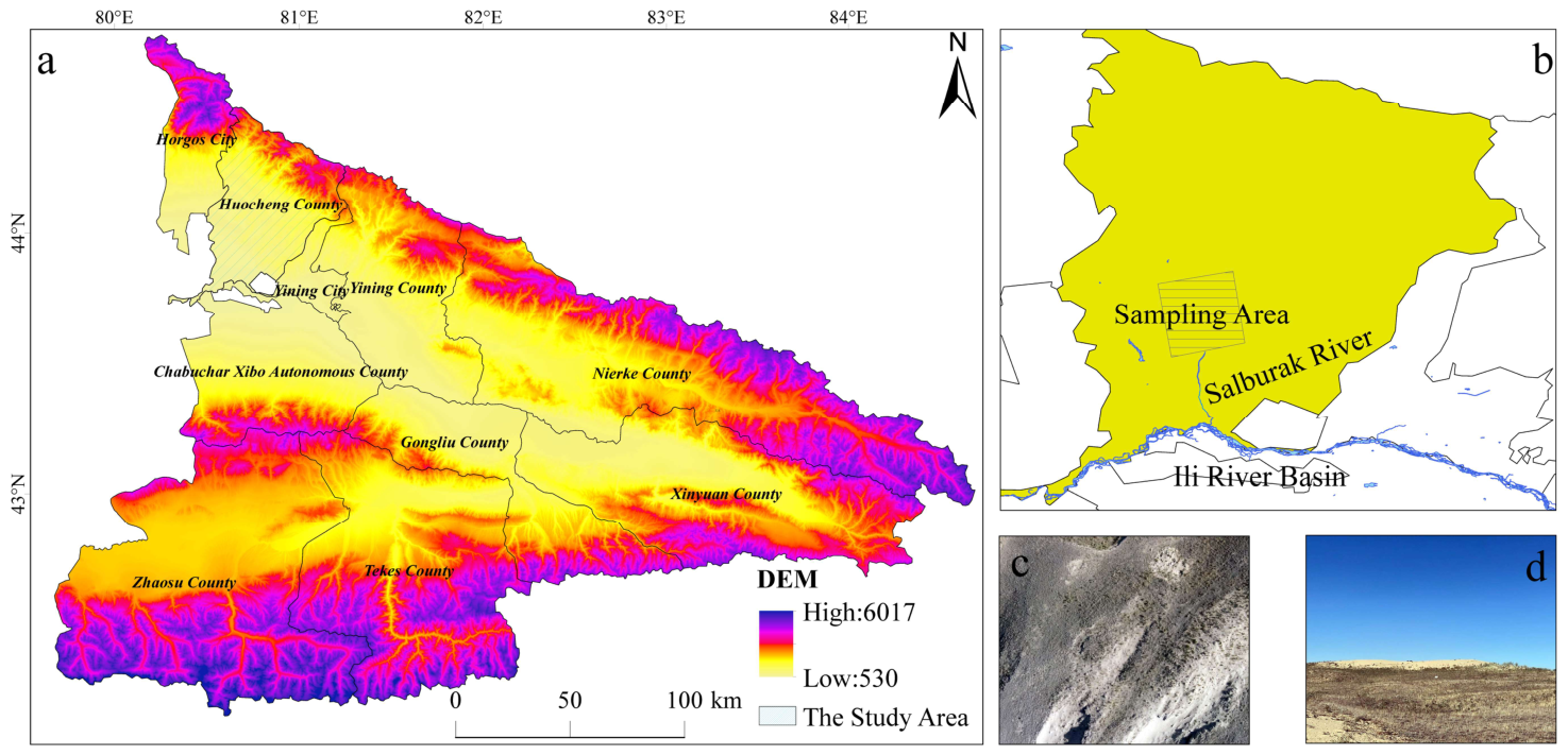
The Sarbulak River Basin is located on the southern slope of the Keguqin Mountain, a branch of the Tianshan Mountains, in the northeastern Huocheng County, Ili Kazakh Autonomous Prefecture, Xinjiang Uygur Autonomous Region, China (43°56′–44°27′ N, 80°50′–81°24′ E). Stretching approximately 59 km from north to south and 36 km from east to west, the basin is a first-order tributary among numerous streams in the Ili River Valley [30]. It is adjacent to the Piliqing River in the northeast and the Guozigou Valley in the northwest. Its northern boundary follows the watershed of the Keguqin Mountain, bordering Bole City of Bortala Mongolian Autonomous Prefecture, while the Ili River separates the basin from the main urban area of Huocheng County to the south (Figure 1). The study area features a temperate continental desert climate. The annual mean temperature is 9.1 °C, with an average diurnal temperature range of 13–15 °C. Annual precipitation ranges from 140 mm to 450 mm, annual evaporation reaches 1400–1900 mm, and annual sunshine duration varies between 2550 h and 3000 h. The annual average wind speed is around 5 m/s, with prevailing winds from the southwest and west–southwest directions [31]. With true north set as 0°, patch long-axis azimuths fall within 66.02–107.22° (mean = 85.06°), demonstrating a general northeast stretching pattern. It matches the characteristics of prevailing southwest and west–southwest valley wind circulation in the Sarbulak River Basin. This directional feature is consistent with the dominant southwest and west–southwest valley wind circulation across the Sarbulak River Basin. It should be noted that the regional annual average wind speed of approximately 5 m/s cited in this study is derived from long-term observations at the standard 10 m height of regional meteorological stations. The 1 km gridded wind speed product (National Cryosphere Desert Data Center, Lanzhou, China) adopted in this study simulates near-surface wind speed at 2 m above the ground. Due to frictional drag from the underlying surface, near-ground wind speed is markedly lower than observations at 10 m height. Accordingly, the value range of the gridded dataset is only 1.23–2.24 m/s. The wind speed interval of 2.10–2.15 m/s identified by the model as favorable for wind erosion also corresponds to the multi-year average wind speed at 2 m height. The discrepancy originates from different observation heights and statistical baselines, rather than data inconsistency. Aeolian landforms are dominated by wind erosion and wind accumulation types, and the desert area within this basin is continuously expanding [32].

2.2. Data Sources and Preprocessing

A close-range aerial survey of mountain sandy patches was carried out in October 2024 using a DJI Phantom 4 Pro UAV (SZ DJI Technology Co., Ltd., Shenzhen, China). Fully automated flight trajectories were pre-planned on the GS Pro flight control platform. All aerial surveys were conducted during clear, windless days with good visibility to ensure high-quality imagery. To generate centimeter-level high-precision topographic data, the relative flight altitude was set to 30 m, with an 80% forward overlap, 60% side overlap, and a flight speed of 5 m/s. Three to four ground control points (GCPs) were evenly distributed within each plot, covering typical landform units such as ridges and gullies. Black circular targets with a diameter of 40 cm were deployed as field markers for GCPs; the center of each target was taken as the reference position, and the precise geographic coordinates of each GCP were measured using a Trimble RTK receiver (Trimble Inc., Westminster, CO, USA). Aerial surveys were completed for four sample plots, yielding a total of 7925 high-resolution images. Agisoft Metashape 2.1.2 (Agisoft LLC, St. Petersburg, Russia, 2024) was adopted for post-processing, including image alignment, GCP registration, camera parameter optimization, dense point cloud generation, mesh construction, and texture mapping. Digital ortho mosaics (DOMs) and digital elevation models (DEMs) were finally produced, both with a consistent output resolution of 2.1 cm.

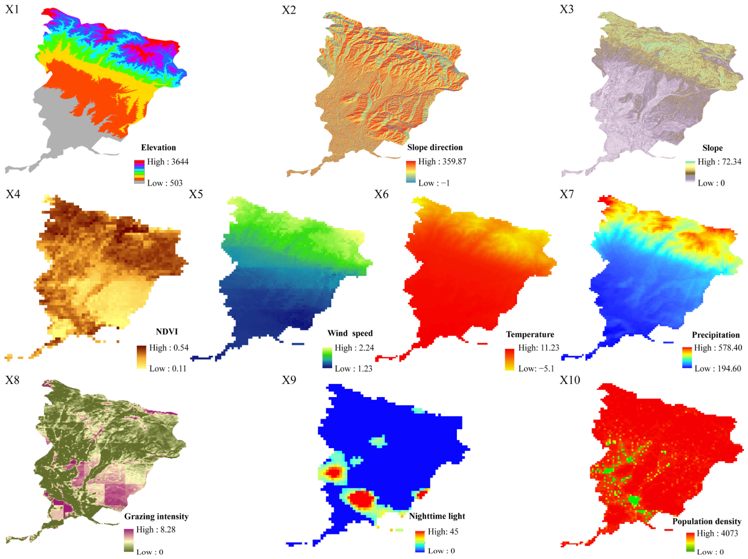
The dynamic evolution of mountain sandy patches is affected by the synergistic effects of multiple factors. The driving factors in this study are divided into two categories: natural elements and human activities, including variables such as topography, climate, grazing intensity, and nighttime light (

Table 2. Driving factors of the study area.

Data Type	Driving Factor	Code	Unit	Spatial Resolution
Topography	Elevation	X1	m	30 m
	Aspect	X2	°	30 m
	Slope	X3	°	30 m
Vegetation	NDVI	X4	-	1 km
Climate	Wind speed	X5	m/s	1 km
	Temperature	X6	°C	1 km
	Precipitation	X7	mm	1 km
Human Activities	Grazing intensity	X8	SU/ha	250 m
	Nighttime light	X9	-	1 km
	Population distribution	X10	Person	1 km

, Figure 2). Temperature and precipitation data were obtained as 1 km resolution raster products from the National Tibetan Plateau Data Center (https://data.tpdc.ac.cn/). The elevation data adopted the ASTER GDEM digital elevation model with a 30 m resolution (https://www.gscloud.cn), from which terrain slope and aspect data were extracted. NDVI data were derived from the MOD13A3 product provided by the National Aeronautics and Space Administration (NASA) (http://glovis.usgs.gov/), with a spatial resolution of 1 km. The nighttime light dataset was generated by integrating DMSP-OLS and SNPP-VIIRS data to produce calibrated DMSP-OLS-like data covering China at a 1 km spatial resolution [33]. Grazing intensity data with a 250 m spatial resolution were acquired from the Figshare platform (https://doi.org/10.6084/m9.figshare.26195684). Wind speed raster data were sourced from the National Cryosphere Desert Data Center (https://www.ncdc.ac.cn/). Population distribution data were obtained from Oak Ridge National Laboratory (ORNL), U.S. Department of Energy (https://landscan.ornl.gov). Field UAV surveys of mountain sandy patches were conducted in October 2024. August 2025 only represents the unified time for batch downloading multi-source raster datasets in this study, rather than the observation period of environmental covariates. To match the long-term wind erosion background of sandy patches and align with the temporal scale of field aerial surveys, unified rules for temporal matching and aggregation were formulated for all environmental factors. Daily raster datasets of temperature, precipitation, and wind speed were firstly aggregated into annual mean values, and then the arithmetic mean from 2018 to 2023 was calculated to construct multi-year climatic composite datasets. The Normalized Difference Vegetation Index (NDVI) was derived from monthly composite products during 2018–2023. Annual Maximum Value Composite (MVC) was adopted to obtain annual optimal vegetation information, followed by the calculation of the 6-year arithmetic mean to generate multi-year vegetation cover composite datasets. Nighttime light and population density data were obtained from annual raster products spanning 2018–2023, and the 6-year arithmetic mean was directly calculated to produce multi-year steady-state background datasets. Grazing intensity adopted the 2024 annual composite dataset, which is fully consistent with the year of UAV field surveys.

All raster datasets were preprocessed uniformly in ArcGIS 10.8, including clipping, resampling, and projection transformation. All data were projected to the Gauss–Krüger coordinate system based on the China Geodetic Coordinate System 2000 (CGCS2000) and resampled to a unified analytical resolution of 250 m. Among these datasets, NDVI, temperature, precipitation, wind speed, population density, and nighttime light have an original spatial resolution of 1 km. Interpolation-based resampling of coarse-resolution grids only achieves numerical smoothing and fitting and cannot generate authentic native spatial information at the 250 m scale. Resampling methods were selected according to variable types: bilinear interpolation was applied for continuous environmental variables, while the nearest neighbor assignment method was used for categorical topographic metrics including elevation, slope, and aspect.

After removing outliers and invalid observations, a total of 1240 mountain sandy patch samples were retained for modeling. Affected by scale mismatch, the four detailed UAV survey plots are far smaller than 1 km climatic raster cells. Numerous sandy patch points fall within the same climatic grid and share identical values of climatic and anthropogenic environmental variables, resulting in obvious spatial pseudo-replication bias. Statistical results indicate that the study area covers only 23 independent 1 km climatic pixels, and the number of unique environmental covariate combinations corresponding to all sampling points is merely 398. Therefore, the effective independent sample size is significantly lower than the total sample size used for modeling.

2.3. Research Methods

2.3.1. Delineating Boundaries of Mountain Sandy Patches

In this study, boundaries of mountain sandy patches were manually delineated via visual digitization in ArcGIS based on high-resolution unmanned aerial vehicle (UAV) digital ortho mosaics (DOMs). The discrimination among sandy patches, vegetation, and bedrock depended on bare sand tone, surface texture, and microtopography. A unified interpretation rule was formulated: only continuously exposed sandy surfaces were defined as sandy patches. Standard specifications were implemented during digitization. The minimum mapping unit was set to 0.5 m², and scattered sand patches smaller than this threshold were excluded. Spatially connected sandy areas were merged into an individual patch, and enclosed vegetation islands within patches were excluded from patch coverage. Moderate boundary smoothing was applied after digitization to eliminate jagged contours caused by manual tracing. To reduce human interpretation errors, quality control was conducted through independent digitization by two interpreters followed by mutual cross-checking. Random samples were selected for accuracy assessment, with field survey points and high-resolution ortho mosaics serving as reference data. Precision, Recall, Intersection over Union (IoU), and relative area error were adopted as evaluation metrics. The assessment yielded Precision = 0.92, Recall = 0.89, and IoU = 0.87. Statistical results for each sample are provided in

Table 3. Accuracy statistics of manually delineated sandy patch boundaries.

Sample ID	Reference Area (m2)	Digitized Area (m2)	Precision	Recall	IoU	Relative Area Error (%)
1	35.99	36.42	0.91	0.88	0.88	1.18
	26.83	26.48	0.92	0.91	0.87	1.28
	171.04	168.24	0.93	0.88	0.87	1.64
	17.86	17.91	0.91	0.88	0.88	0.31
2	75.82	76.82	0.91	0.90	0.86	1.32
	75.43	75.08	0.91	0.90	0.87	0.46
	159.6	164.21	0.94	0.89	0.86	2.88
3	28.12	28.43	0.94	0.88	0.84	1.11
	23.88	23.86	0.93	0.89	0.86	0.11
	58.51	58.13	0.93	0.9	0.88	0.65
4	9.31	9.22	0.93	0.88	0.88	0.94
	49.05	49.72	0.94	0.88	0.87	1.37
Mean	—	—	0.92	0.89	0.87	1.10

Precision = TP/(TP + FP); Recall = TP/(TP + FN); and IoU = TP/(TP + FP + FN). Relative area error = |Digitized area − Reference area|/Reference area × 100%. TP = overlapping area between manually digitized patches and reference data; FP = over-extracted area; and FN = omitted area.

.

2.3.2. Kruskal–Wallis H Test (Non-Parametric One-Way Analysis of Variance)

Inter-group difference tests were performed on morphological parameters of sandy patches. As the morphological parameters failed to meet the normality assumption, the Kruskal–Wallis H test (non-parametric one-way analysis of variance) was adopted, and its formula is expressed as:

$$\mathrm{H}={\displaystyle \frac{12}{N(N+1)}}{\sum }_{i=1}^k{\displaystyle \frac{R_i^2}{n_i}}-3(N+1)$$

(1)

where N is the total number of samples; k represents the number of groups; $n_i$ denotes the sample size of the i-th group; and $R_i$ is the sum of ranks for samples in the i-th group. A corrected formula was applied in the presence of tied ranks. If significant inter-group differences were detected, Dunn’s post hoc multiple comparisons with Bonferroni correction were conducted, and the effect size ${\eta }^2$ was calculated to quantify the magnitude of differences.

2.3.3. Extraction and Analysis of Morphological Characteristics

Drawing on previous studies on the extraction of morphological parameters of sand dunes [34], based on UAV orthophotos, eight morphological parameters of sandy patches, including length (L), width (W), height (H), perimeter (C), base area (S), surface area (U), volume (V), and length–width ratio (L/W), were calculated using ArcGIS. Considering the heavy workload, only representative mountain sandy patches within the four sampling plots were selected for parameter extraction. Specifically, 16 patches were obtained in Plot 1, 39 in Plot 2, 14 in Plot 3, and 23 in Plot 4, yielding a total of 92 independent geomorphic sandy patches. Based on statistical theory, SPSS 27.0 was adopted to conduct Pearson correlation analysis on the morphological parameters of mountain sandy patches, and significance tests were performed on correlation coefficients.

2.3.4. Principal Component Analysis

To eliminate multicollinearity inherent to geometric morphological metrics and unpack the intrinsic structural characteristics of sandy patches, principal component analysis (PCA) was conducted on eight morphological indicators: major axis length (L), width (W), height (H), perimeter (C), base area (S), surface area (U), volume (V), and length–width ratio (L/W).

All variables were standardized via Z-score transformation to eliminate dimensional disparities:

$$Z_{ij}={\displaystyle \frac{x_{ij}-{\overline{x}}_j}{{\sigma }_j}}$$

(2)

where $Z_{ij}$ is the standardized value of the j-th indicator for the i-th sandy patch; $x_{ij}$ is the raw observation; and ${\overline{x}}_j$ and ${\sigma }_j$ denote the mean and standard deviation of the j-th indicator, respectively.

Each principal component was defined as a linear weighted combination of standardized variables:

$${PC}_k=a_{k1}{z}_1+a_{k2}{z}_2+\cdots +a_{k8}{z}_8$$

(3)

in which ${PC}_k$ represents the k-th principal component; $a_{k1}$~$a_{k8}$ are eigenvector loadings; and $z_1$~$z_8$ are eight standardized morphological metrics.

The explanatory capacity of each component was quantified by variance contribution:

$$V_k={\displaystyle \frac{{\lambda }_k}{{\sum }_{j=1}^8{\lambda }_j}}\times 100\%, {CV}_k={\sum }_{i=1}^k{V}_i$$

(4)

where $V_k$ is the individual variance contribution rate of the k-th component; ${CV}_k$ is the cumulative variance contribution rate; and ${\lambda }_k$ stands for eigenvalue.

The KMO test and Bartlett’s sphericity test were implemented to verify dataset suitability for PCA. Principal components were extracted under the threshold of eigenvalue λ > 1, and loadings, eigenvalues, and variance explained ratios were exported. Notably, PCA was only utilized to interpret morphological differentiation patterns.

2.3.5. Spearman Rank Correlation Analysis

Environmental predictors contain extreme outliers and exhibit significantly skewed distributions, which fail to meet the assumptions of parametric tests; therefore, Spearman rank correlation was adopted for analysis. As a non-parametric test, Spearman rank correlation can effectively characterize monotonic associations between variables [35]. Importantly, this method only reflects monotonic statistical covariation within the sample dataset and cannot reflect real causal interactions between geomorphic variables, and its calculation formula is given as follows:

$$r_s=1-{\displaystyle \frac{6{\displaystyle {\sum }_{i=1}^n}{d}_i^2}{n\left(n^2-1\right)}}$$

(5)

where $r_s$ denotes the Spearman correlation coefficient; $n$ represents the sample size; and $d_i$ refers to the rank difference of paired observations between the two variables.

2.3.6. XGBoost Model

To reveal the nonlinear response relationships between the distribution of mountain sandy patches and topographic, climatic, vegetation, and human activity factors, this study adopted the XGBoost ensemble learning algorithm to construct a prediction model for quantitatively interpreting environmental responses of sandy patches. In this study, the presence or absence of mountain sandy patches was defined as the response variable Y to establish a binary classification model. Specifically, sampling points inside sandy patches were assigned (Y = 1) (presence), while control points outside sandy patches were assigned (Y = 0) (absence). All environmental predictors were averaged within a 5 m buffer surrounding each sampling point to ensure consistent spatial support between the response variable and environmental covariates. XGBoost is a scalable ensemble technique based on gradient boosting, which has been proven to be a reliable and efficient solver for machine learning tasks [36]. As an ensemble learning algorithm built on the gradient boosting framework, XGBoost delivers outstanding computational and predictive performance via multiple optimization strategies [37]. This algorithm integrates an efficient parallel computing mechanism and regularization methods, greatly improving model robustness while effectively mitigating overfitting [38]. For model reproducibility, the complete modeling workflow is elaborated as follows. Firstly, the standardized sample dataset was randomly split into a training set and a test set at a ratio of 7:3. The training subset was only used for hyperparameter tuning and was not adopted for final model evaluation or result interpretation. Secondly, grid search was implemented on the training subset to optimize key hyperparameters including learning rate, maximum tree depth, subsample ratio, and regularization coefficients, with the minimum root mean square error (RMSE) defined as the optimization objective. Formal model evaluation and subsequent analyses were conducted using leave-one-plot-out 5-fold spatial cross-validation to avoid spatial leakage. Under this validation scheme, all samples within a single plot were assigned to the same fold to eliminate bias induced by adjacent samples with similar environmental information.

To further objectively verify the predictive performance of the model, multiple benchmark models including multiple linear regression (MLR), generalized additive model (GAM), and random forest (RF) were constructed for comparative analysis under an identical spatial cross-validation framework. The prediction accuracy of each model is listed in

Table 4. Comparison of predictive performance among different models.

Model	Coefficient of Determination (R2)	Mean Squared Error (MSE)	Root Mean Squared Error (RMSE)
Random Forest (RF)	0.8921	0.2329	0.4826
XGBoost	0.8537	0.3456	0.5879
Generalized Additive Model (GAM)	0.6751	1.3194	1.1486
Multiple Linear Regression (MLR)	0.6124	1.9596	1.4

A higher R² (closer to 1) and lower values of MSE and RMSE indicate better model prediction accuracy. Model comparison metrics were calculated under an identical leave-one-plot 5-fold spatial cross-validation framework.

. The comparison results reveal that tree-based models (XGBoost and random forest) achieve substantially better predictive performance than conventional statistical models. Random forest yields the highest prediction accuracy, while XGBoost exhibits slightly lower accuracy yet favorable generalization ability. Compared with MLR and GAM, both tree-based models possess a stronger capacity to capture the nonlinear relationships between sandy patches and environmental factors. The objective function of the XGBoost model consists of a loss term and a structural regularization term, and the calculation formula of the loss term is expressed as:

$$\mathcal{L}\left(\mathrm{\varnothing }\right)={\displaystyle \sum _{i=1}^n}l\left(y_i,{\widehat{y}}_i\right)+{\displaystyle \sum _{k=1}^K}\Omega \left(f_k\right)$$

(6)

where n is the total number of samples; $y_i$ and ${\widehat{y}}_i$ are the true value and model-predicted value of the i-th sample, respectively; $l\left(y_i,{\widehat{y}}_i\right)$ denotes the loss function, which quantifies the error between predicted values and true values; K refers to the total number of decision trees in the model; $f_k$ represents the k-th decision tree; and $\Omega \left(f_k\right)$ is the structural regularization term for a single tree, which controls model complexity and suppresses overfitting.

The calculation formula of the regularization term is as follows:

$$\mathcal{L}\left(\varphi \right)=\gamma T+{\displaystyle \frac{1}{2}}\lambda {\displaystyle \sum _{j=1}^T}{\mathcal{W}}_j^2$$

(7)

where T is the number of leaf nodes in a single tree; ${\mathrm{W}}_{\mathrm{j}}$ denotes the output weight of the j-th leaf node; $\gamma$ represents the penalty coefficient for the number of leaf nodes; and $\lambda$ is the L2 regularization coefficient.

All modeling, hyperparameter optimization, and subsequent SHAP analysis were programmed with Python 3.10. Core package versions are specified for full reproducibility: XGBoost 1.7.6, SHAP 0.42.1, scikit-learn 1.3.0, NumPy 1.25.2, Pandas 2.0.3, and SciPy 1.11.3. GridSearchCV from scikit-learn was adopted for hyperparameter tuning, and bootstrap resampling functions were implemented via native NumPy codes to calculate 95% confidence intervals of SHAP thresholds.

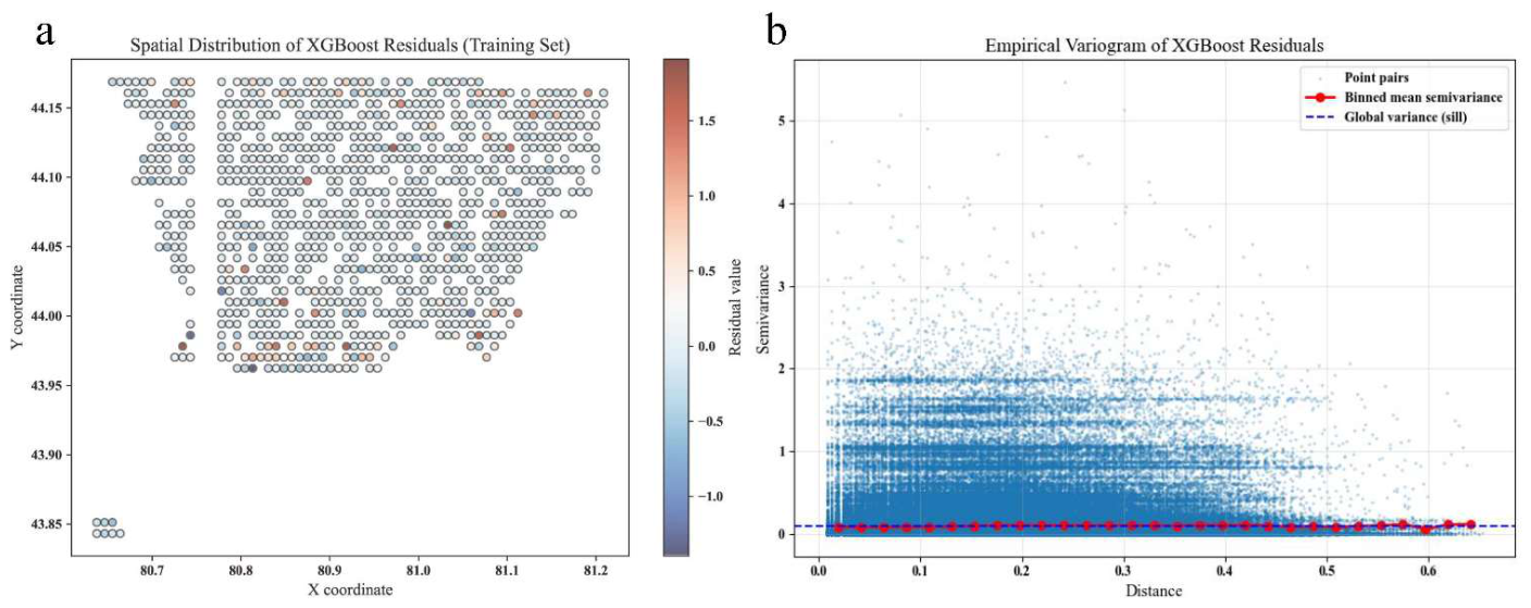
In addition, residual spatial autocorrelation diagnosis was implemented after model training. The global Moran’s I was calculated, and spatial distribution maps of residuals as well as empirical variograms were plotted (Figure 3) to identify potential unexplained spatial structures within the residual field. The spatial distribution map reveals that residuals are randomly distributed without obvious regional clustering. The empirical variogram indicates that the average semivariance does not exhibit a significant upward trend with increasing distance and fluctuates around the global variance. The global Moran’s I equals I = 0.186 with p = 0.117, which further confirms the spatial independence of residuals. These results demonstrate that the established XGBoost model has sufficiently captured spatial dependence embedded in the samples, and no additional spatial regression terms are required.

2.3.7. SHAP Interpretability Analysis

The SHapley Additive exPlanations (SHAP) framework was adopted to interpret the marginal effects of environmental factors in the XGBoost regression model. Normalized mean absolute SHAP values were used to quantify the relative predictive importance of each predictor. Notably, SHAP results only reflect statistical predictive contributions under the current dataset and model configuration and cannot directly represent causal driving proportions in ecological processes. SHAP is a model interpretability framework built based on the game-theoretic Shapley value, which is widely used to quantify the contribution of each feature to the prediction results in machine learning models [39]. This method can assign a corresponding importance score to each feature and clearly explain the internal correlation between input variables and model outputs. Its calculation formula is as follows:

$${\varnothing }_i={\sum }_{S\subseteq N\setminus \left\{i\right\}}{\displaystyle \frac{\left|S\right|!·\left(\left|N\right|-\left|S\right|-1\right)!}{\left|N\right|!}}\left(\upsilon \left(S\cup \left\{i\right\}\right)-\upsilon \left(S\right)\right)$$

(8)

where ${\varnothing }_i$ denotes the SHAP value corresponding to feature i, which characterizes the marginal contribution of this feature to model prediction; N stands for the set consisting of all features; S is the feature subset excluding the i-th feature; $\upsilon \left(S\right)$ represents the contribution of feature subset S to the model prediction output; and $\upsilon \left(S\cup \left\{i\right\}\right)$ refers to the predictive contribution after adding feature i into subset S.

To assess the uncertainty of SHAP importance rankings induced by multicollinearity, multi-layer stability validation was carried out. Hierarchical clustering based on Spearman correlation coefficients was performed to identify clusters of highly correlated variables. XGBoost models were reconstructed after sequentially removing a single variable from each collinear cluster to compare the rankings of relative predictive importance. A total of 100 bootstrap resampling runs with replacement were implemented to obtain the ranking distribution of each factor and the 95% confidence intervals of normalized mean absolute SHAP values. Permutation importance tests were further applied to cross-verify the robustness of rankings. All stability test results are shown in

Table 5. Stability tests of SHAP importance ranking and Bootstrap confidence intervals.

Predictive Features	Test1	Test2	Test3	Test4	Test5	Test6	Confidence Interval
X5	1	1	1	—	1	1	0.375–0.641
X7	2	2	2	2	2	2	0.181–0.370
X1	3	—	4	4	4	5	0.130–0.253
X6	4	3	3	1	4.5	3	0.092–0.262
X4	5	5	6	3	4.5	4	0.112–0.253
X8	6	4	5	5	5	6	0.109–0.249
X9	7	8	7	7	8	8	0.020–0.070
X10	8	6	8	6	7	7	0.022–0.121
X2	9	7	—	8	9	9	0.015–0.252
X3	10	9	9	9	10	10	0.009–0.028

Values in the table indicate the importance rank of predictors; smaller values correspond to higher relative predictive importance. The symbol “—” means the variable was excluded and not incorporated into the model. Test1: full-variable original model; Test2–Test4: modeling results after removing highly correlated variables; Test5: median importance rank derived from 100 bootstrap resampling runs; Test6: ranking based on permutation importance; and95% confidence interval of normalized mean absolute SHAP values (2.5th quantile–97.5th quantile). Wind speed and precipitation consistently occupy the top two ranks under all full-variable modeling scenarios. After removing wind speed, the predictive importance of temperature (highly collinear with wind speed) increases remarkably, indicating the redistribution of SHAP importance among collinear predictors. NDVI generally falls within the top 5 with minor fluctuations in ranking.

.

3. Results

3.1. Morphological Parameter Variations of Mountain Sandy Patches

3.1.1. Basic Information of Sample Plots

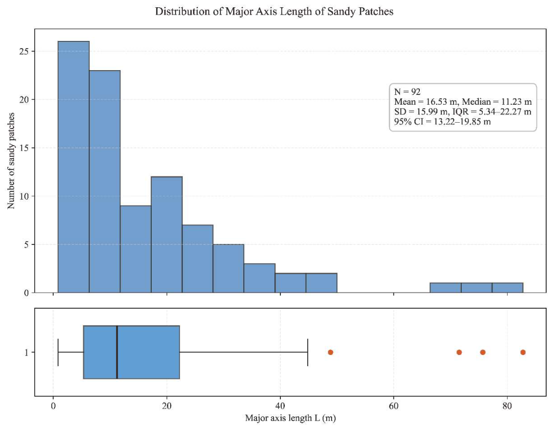
Global descriptive statistics of patch major axis length were calculated based on all 92 sandy patches: N = 92, mean = 16.53 m, median = 11.23, standard deviation = 15.99 m, and interquartile range = 5.34~22.27 m. The major axis length shows a prominent right-skewed distribution. Most sandy patches have relatively small major axis lengths, and a small number of oversized patches increase the arithmetic mean; the distribution characteristics are illustrated in Figure 4. Mountain sandy patches in the study area are predominantly distributed along the ridgelines of the Keguqin Mountains. Four sampling plots were arranged using stratified purposive sampling, covering low, medium, and high elevation gradients, gentle to steep slopes, and sunny and shady aspects, as well as different levels of NDVI and grazing intensity. The sampling plots cover two typical geomorphic units (ridges and gullies) to capture comprehensive environmental gradients across the watershed (

Table 6. Basic information of four sampling plots in the Sarbulak River Basin.

Sample Plot	1	2	3	4
Central Coordinates	44°6′6.834″ N	44°6′27.858″ N	44°6′43.529″ N	44°7′1.221″ N
	80°52′19.351″ E	80°52′35.918″ E	80°52′55.435″ E	80°52′57.937″ E
Sample Area/km2	0.028	0.533	0.054	0.075
Distribution Density (patches/km2)	563.98	73.17	257.03	307.23

Distribution density = number of mountain sandy patches per square kilometer. Coordinates adopt a WGS84 geographic coordinate system. Total sample size (n = 92) measured sandy patches across all plots.

). Constrained by field accessibility and the heavy workload of UAV aerial surveys, the area of each sampling plot is limited, which leads to sampling uncertainty when extrapolating the conclusions to the entire basin. The number of acquired UAV images is 305 for Plot 1, 4260 for Plot 2, 3055 for Plot 3, and 305 for Plot 4. Plot 2 possesses the largest spatial coverage, while Plot 1 has the highest distribution density of mountain sandy patches.

3.1.2. Spatial Morphology of Mountain Sandy Patches

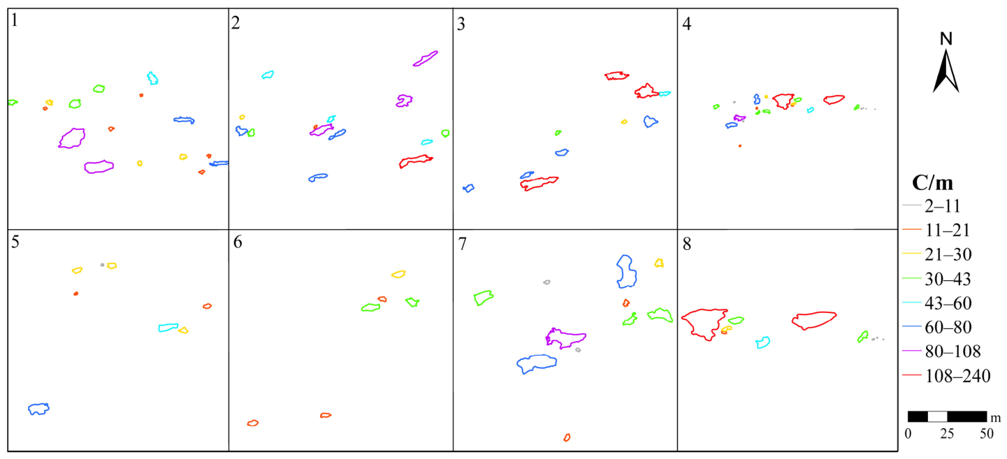
Based on the aerial orthophotos of the four sample plots, thematic maps of mountain sandy patches were produced (Figure 5). Given the varying distributions of mountain sandy patches across each plot, all patches were classified into eight groups. Group 1 corresponds to Sample Plot 1; Groups 2, 3, and 4 belong to Sample Plot 2; Groups 5 and 6 belong to Sample Plot 3; and Groups 7 and 8 belong to Sample Plot 4. In Sample Plot 1, mountain sandy patches are dominated by elliptical, circular, and elongated shapes with relatively concentrated distribution. Approximately 69% of the patches are elliptical and located adjacent to hills; about 29% occur on hilltops and mostly present an elongated shape. The perimeters of the sandy patches fluctuate slightly overall, ranging from a minimum of 2 m to a maximum of 90 m, with an average perimeter of 38.92 m. Sample Plot 2 contains the largest number and larger individual sizes of mountain sandy patches, exhibiting significantly better overall development than the other plots. The patches are mainly elongated and irregular polygons are predominantly distributed in the northeastern and northwestern parts of the plot, with sparse coverage in the central area. Around 31% of the patches feature irregular outlines, while the rest are elongated. Their perimeters vary from 11 m to 240 m, with an average of 75.64 m. In Sample Plot 3, mountain sandy patches are sparsely distributed and mostly situated beside hills, with only roughly 20% occurring in inter-hill depressions. Irregular shapes prevail here, yet the range of patch perimeters is the narrowest among all plots: the maximum perimeter is 60 m and the minimum is 11 m, yielding an average perimeter of 26.39 m. For Sample Plot 4, the perimeters of mountain sandy patches show substantial variation. Roughly 85% of patches lie on hills, and few are found in inter-hill zones. The patch perimeters span from 2 m up to 240 m, with an average value of 35.94 m.

The Kruskal–Wallis H test results (

Table 7. Test results of inter-plot differences in the morphological parameters of sandy patches.

Parameters	H	p	η2	Significance
L/m	22.689	<0.001	0.224	***
W/m	24.105	<0.001	0.24	***
H/m	9.342	0.025	0.072	*
C/m	25.512	<0.001	0.256	***
S/m2	24.300	<0.001	0.242	***
U/m2	23.410	<0.001	0.232	***
V/m3	19.268	<0.001	0.185	***
L/W	4.326	0.228	0.015	ns

*** (p < 0.001); * (p < 0.05); and ns indicates a non-significant difference (p ≥ 0.05).

) indicated that all morphological parameters exhibited significant inter-plot differences (p < 0.05), except for the length–width ratio (L/W). Perimeter (C), width (W), base area (S), surface area (U), major axis length (L), and volume (V) showed highly significant differences (p < 0.001), with effect sizes (η²) ranging from 0.185 to 0.256, representing large effects. Height (H) differed significantly among plots (p = 0.025), (η² = 0.072), corresponding to a moderate effect. No significant difference was detected for the length–width ratio (p = 0.228), η² = 0.015). Elongated shapes dominate mountain sandy patches across all four sample plots, while circular, elliptical, and irregular polygonal shapes appear in partial areas. Among all plots, Sample Plot 2 has the largest quantity and maximum perimeter of sandy patches, demonstrating the optimal development status compared with the other three plots. Sample Plot 1 covers the smallest area yet boasts the most concentrated distribution of sandy patches. Approximately 50% of all sandy patches of elongated, circular, elliptical, and irregular polygonal shapes are distributed on hills, 40% of patches with the same morphological types are located adjacent to hills, and the remaining 10% occur in inter-hill depressions.

3.1.3. Statistical Features of Morphological Parameters for Mountain Sandy Patches

Statistical results reveal significant differences in the morphological parameters of mountain sandy patches across the four sample plots (

Table 8. Morphological parameters of mountain sandy patches.

Sample Plot		L/m	W/m	H/m	C/m	S/m2	U/m2	V/m3	L/W
1	Maximum	32.93	20.01	3.96	90.61	448.62	455.47	286.94	8.96
	Minimum	1.98	2.10	0.02	11.42	5.08	4.31	0.16	0.46
	Mean	11.77	6.52	0.67	38.92	83.64	85.56	48.82	2.18
2	Maximum	82.78	28.70	3.94	240.72	1539.26	1577.18	1975.13	6.74
	Minimum	3.28	2.23	0.02	17.09	14.11	13.61	4.51	0.29
	Mean	24.68	10.51	1.19	75.64	255.82	270.81	339.42	2.58
3	Maximum	20.61	10.38	2.70	63.33	175.92	275.60	256.31	4.14
	Minimum	2.07	0.63	0.01	6.43	1.65	1.52	0.05	0.90
	Mean	8.89	4.48	0.79	26.39	41.21	49.69	47.83	2.20
4	Maximum	43.60	33.71	1.79	145.43	850.37	994.65	296.47	4.47
	Minimum	0.85	0.29	0.02	2.38	0.27	0.08	0.02	0.35
	Mean	10.69	5.95	0.56	35.94	100.40	107.89	56.32	2.07

L = length; W = width; H = height; C = perimeter; S = base area; U = surface area; and V = volume. All values are presented as raw extreme and mean values of measured patches; error terms of morphological parameters are standard deviation (SD).

). Except for L, W, and H, other morphological parameters fluctuate drastically within each plot. For instance, the average value of V in Sample Plot 2 reaches 339.42 m³, while the mean U value of Sample Plot 3 is only 49.69 m². Nevertheless, the average values of W, H, and L/W are relatively consistent among all sample plots.

3.1.4. Relationships Among Morphological Parameters of Mountain Sandy Patches

Pearson correlation analysis was conducted on the morphological parameters of 92 mountain sandy patches (

Table 9. Correlation analysis of morphological parameters of sandy patches.

	L/m	W/m	H/m	C/m	S/m2	U/m2	V/m3	L/W
L/m	1
W/m	0.619 **	1
H/m	0.169	0.243 *	1
C/m	0.945 **	0.772 **	0.240 *	1
S/m2	0.893 **	0.763 **	0.125	0.923 **	1
U/m2	0.886 **	0.772 **	0.121	0.926 **	0.996 **	1
V/m3	0.680 **	0.531 **	0.520 **	0.762 **	0.736 **	0.730 **	1
L/W	0.510 **	−0.158	0.013	0.352 **	0.213 *	0.208 *	0.185	1

** Indicates the correlation is significant at the 0.01 level (two-tailed) and * indicates the correlation is significant at the 0.05 level (two-tailed). n = 1240 independent sandy patch samples. L = length; W = width; H = height; C = perimeter; S = base area; U = surface area; and V = volume.

). The results show that most pairwise combinations of scale-related parameters, including major axis length (L), width (W), perimeter (C), base area (S), surface area (U), and volume (V), exhibit highly significant correlations at (p < 0.01). Height (H) presents generally weak correlations with other morphological indicators, whereas the length–width ratio (L/W) shows non-significant correlations with multiple parameters. Specifically, height has no significant correlation with major axis length, base area, and surface area, and is only significantly correlated with width and perimeter at (p < 0.05). The correlation pattern of the length–width ratio also displays obvious heterogeneity. It is not significantly correlated with width, height, and volume; it is highly significantly correlated with major axis length and perimeter at (p < 0.01), and significantly correlated with base area and surface area at (p < 0.05). A unified classification criterion for correlation strength was adopted: |r| < 0.3 denotes weak correlation, (0.3 ≤ |r| ≤ 0.7) moderate correlation, and |r| > 0.7 strong correlation. Under this criterion, the correlation coefficient between volume and major axis length (r = 0.680**) is defined as a moderate correlation, which revises the previous incorrect classification as a weak correlation. Major axis length, perimeter, base area, surface area, and volume are generally strongly intercorrelated. Such high covariation originates from the inherent mathematical coupling of geometric metrics, rather than evidence for geomorphic processes of synergistic expansion and balanced development of mountain sandy patches. To mitigate analytical interference caused by geometric multicollinearity and extract independent morphological dimensions of sandy patches, principal component analysis was further implemented in this study.

To clarify the intrinsic morphological structure of mountain sandy patches and eliminate multicollinearity among geometric indicators, principal component analysis (PCA) was performed on eight morphological parameters. The KMO test and Bartlett’s sphericity test verified the suitability of the dataset for PCA. Following the extraction criterion of eigenvalue > 1, three valid principal components were retained, with a cumulative explained variance of 93.3%, which sufficiently captured the core information of original morphological variables (

Table 10. Principal component analysis of the morphological parameters of mountain sandy patches.

Indicator	PC1	PC2	PC3
L/m	0.94	0.283	−0.008
W/m	0.791	−0.41	0.289
H/m	0.303	−0.489	−0.8
C/m	0.985	0.075	0.028
S/m2	0.967	0.017	0.199
U/m2	0.967	0.012	0.208
V/m3	0.827	−0.186	−0.336
L/W	0.304	0.85	−0.401
Eigenvalue	5.217	1.25	1.08
Variance explained (%)	64.51	15.46	13.35
Cumulative variance explained (%)	64.51	79.96	93.31

KMO = 0.715; Bartlett’s sphericity test: X² = 2925.75, p < 0.001. Principal components were extracted based on the criterion of eigenvalue > 1.

). The first principal component (PC1) exhibited high positive loadings on perimeter, base area, surface area, major axis length, volume, and width. As the primary dimension controlling morphological differentiation, PC1 represented the overall scale of sandy patches and accounted for 64.5% of total morphological variation. The second principal component (PC2) had a prominent positive loading on length–width ratio and negative loadings on width and height, reflecting planar contour features; higher scores of PC2 corresponded to more elongated patch shapes. The third principal component (PC3) carried a strong negative loading on height and characterized vertical development of sandy patches, with lower scores indicating more remarkable three-dimensional features. PCA separated three mutually independent morphological dimensions, namely patch scale, planar contour, and vertical development, and greatly reduced data redundancy induced by inherent mathematical coupling of geometric metrics, providing comprehensive independent indicators for morphological differentiation analysis. It should be noted that the extracted principal components were only adopted to interpret morphological differentiation rules, rather than incorporated into the subsequent XGBoost driving factor model; raw environmental and morphological variables were retained for modeling.

3.2. Analysis of Driving Factors

3.2.1. Accuracy Verification of XGBoost Model

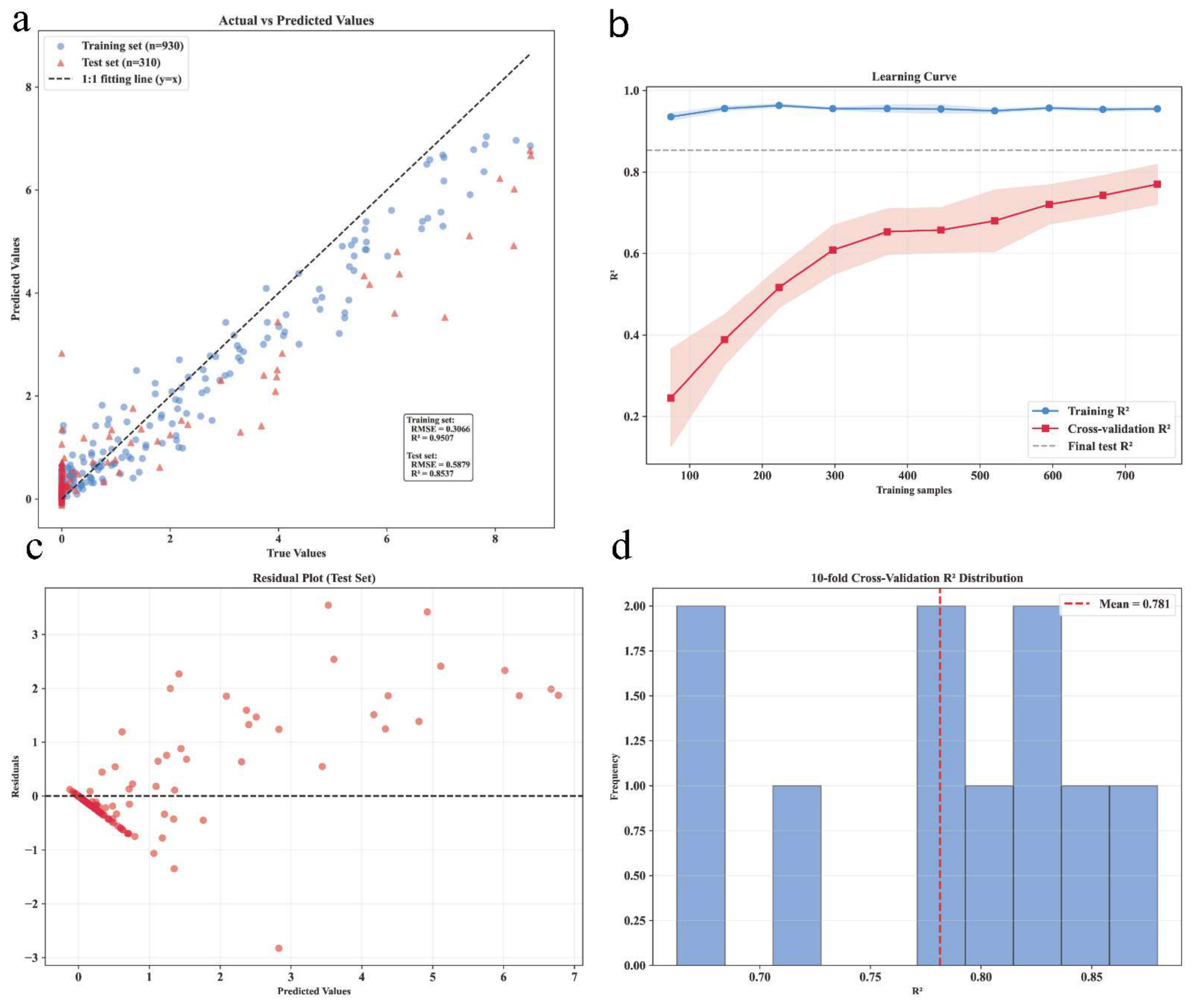
In this study, the XGBoost regression model was implemented based on Python. The dataset was split into a training set and a test set at a ratio of 7:3. Five-fold cross-validation combined with grid search was adopted to optimize hyperparameters, and an early stopping strategy was introduced to tune the number of iterations. The results are presented in Figure 6a. The final optimal parameters of the model are as follows: maximum tree depth of 7, learning rate of 0.01, iteration count of 300, subsample rate of 0.8, column sample rate of 0.8, L1 regularization coefficient of 0, and L2 regularization coefficient of 1. The test set yielded an R² of 0.8537 and an RMSE of 0.5879. Based on the results of leave-one-plot-out spatial cross-validation, the difference in R² between the training set and test set is 0.097, which is less than 0.1, and the standard deviation of cross-validated R² equals 0.072. Comprehensive diagnosis relying on learning curves, residual scatter plots, and cross-validation error histograms (Figure 6b–d) reveals slight model overfitting. Nevertheless, the model exhibits good overall generalization ability with relatively limited fluctuations in prediction accuracy. Overall, the model exhibits satisfactory fitting performance and can be applied for subsequent analysis.

3.2.2. Correlation Analysis Among Driving Factors

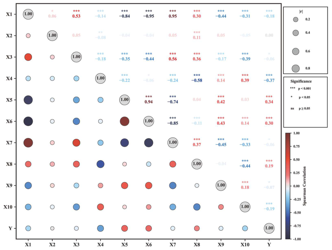
Spearman correlation analysis was adopted to explore the statistical correlation characteristics between each driving factor and mountain sandy patches (Figure 7). The results show that X5 and X6 have extremely significant positive correlations with mountain sandy patches, with correlation coefficients of 0.34 and 0.30, respectively. This indicates that higher wind speed and air temperature promote the development of mountain sandy patches. In contrast, X4 presents an extremely significant negative correlation with mountain sandy patches, with a correlation coefficient of −0.37, which reveals that NDVI exerts an obvious inhibitory effect on sandy patches.

3.2.3. Contribution of Driving Factors to Mountain Sandy Patches

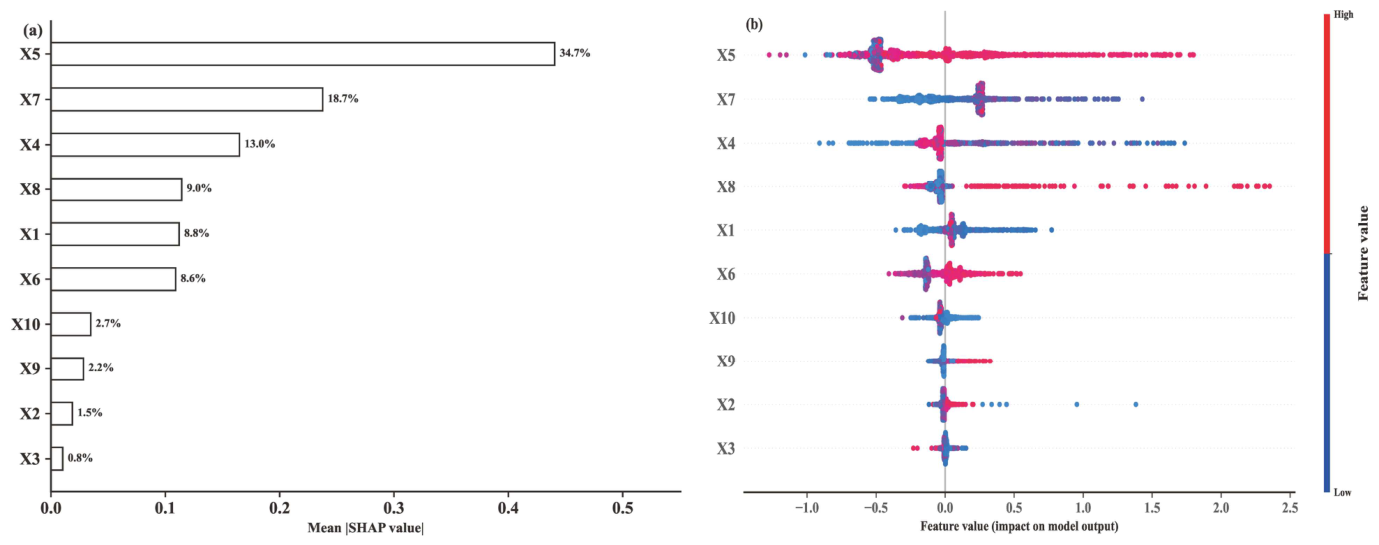
This study integrates the XGBoost model with the SHAP interpretability framework to quantify the magnitude and variation trends of environmental predictors affecting mountain sandy patches (Figure 8). Based on the ranking of normalized mean absolute SHAP values (Figure 8a), the influencing intensity of each factor in descending order is wind speed (X5), precipitation (X7), NDVI (X4), grazing intensity (X8), elevation (X1), temperature (X6), population distribution (X10), nighttime light (X9), aspect (X2), and slope (X3). Wind speed presents the highest relative predictive contribution, accounting for 34.7% of the total SHAP magnitude, followed by precipitation (18.7%) and NDVI (13.0%). Collectively, these three dominant predictors explain more than 66% of the model’s predictive variation.

To further clarify the marginal response characteristics of sandy patches to individual environmental factors, SHAP dependence analyses were performed for all samples (Figure 8b). Each scatter point represents an individual factor value, and the corresponding SHAP value reflects its positive or negative marginal effect on sandy patch development. In general, promoting factors exhibit a “blue-left and red-right” distribution pattern, whereas inhibitory factors show a “red-left and blue-right” pattern. Detailed interpretation indicates that wind speed, grazing intensity, and temperature exert predominant promoting effects on mountain sandy patches. By comparison, precipitation strongly restricts sandy patch development. NDVI shows bidirectional influences across different value ranges, with its regulatory effect shifting from inhibition to promotion along its gradient.

Considering that multicollinearity among environmental predictors may induce uncertainty in SHAP ranking, we conducted systematic stability validation to verify the robustness of the above results. Stability tests covering full-variable modeling, collinear variable exclusion, 100-times bootstrap resampling, and permutation importance evaluation demonstrate that wind speed and precipitation consistently rank as the top two predictors across most scenarios. NDVI stably maintains a top-five predictive importance (ranking 3–6) in all complete variable models. When highly collinear wind speed was excluded, temperature rose to the first rank and NDVI advanced to the third rank, indicating evident substitutable effects between wind speed and temperature. Integrating bootstrap median rankings and permutation importance results, wind speed and precipitation remain the most stable dominant predictors, while NDVI maintains steady predictive performance within the top five. Overall, the core variable rankings show good robustness against multicollinearity and model randomness (Table 5).

3.2.4. Threshold Analysis of Driving Factors

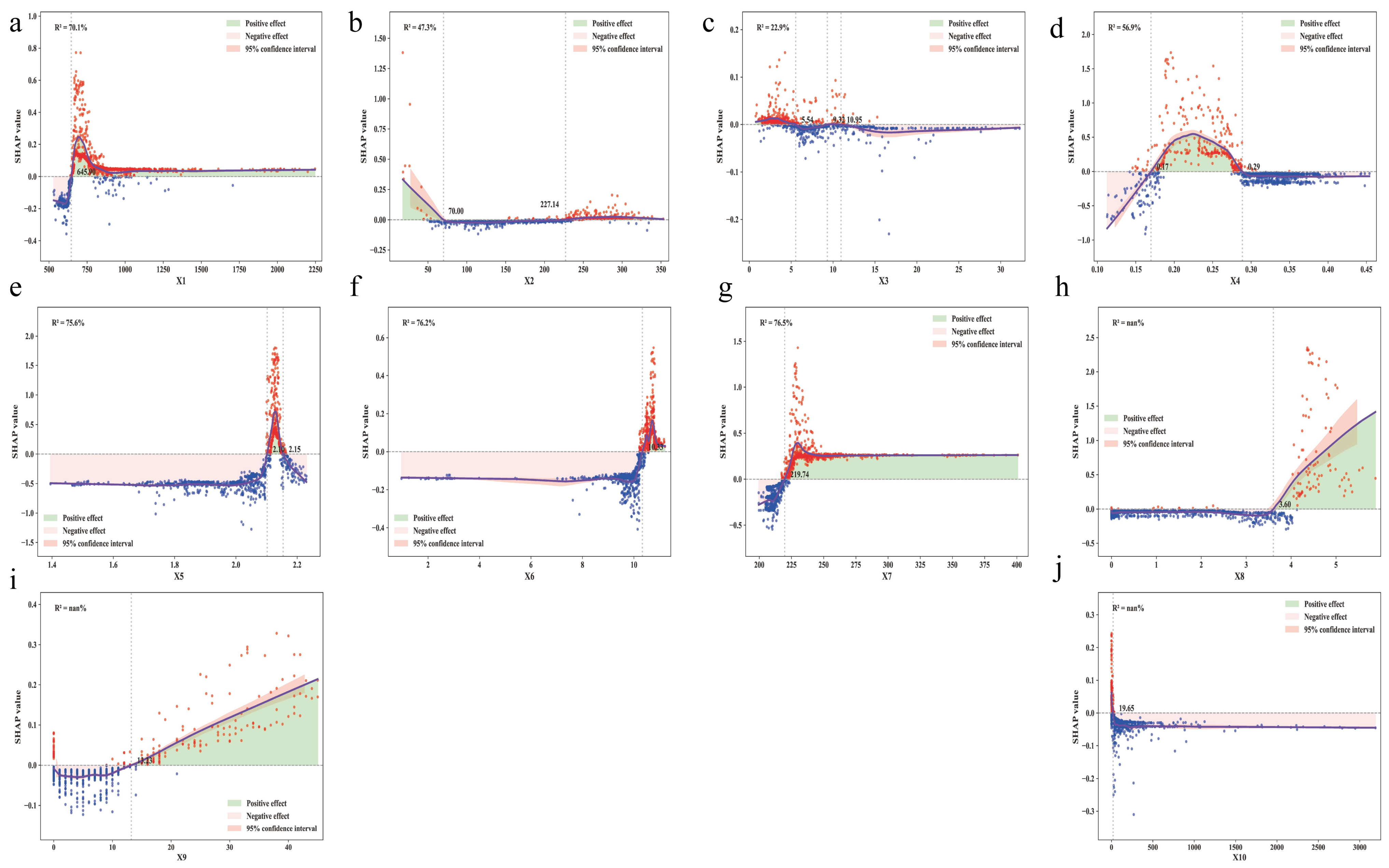
Based on threshold features extracted from SHAP dependence curves, this study analyzes the marginal association intervals between each predictor and mountain sandy patches, and identifies the nonlinear response patterns of all predictors (Figure 9). Each predictor exhibits distinct nonlinear responses, with no universal monotonic threshold transition pattern observed.

Elevation (X1) shows a positive marginal correlation with mountain sandy patches when exceeding the median threshold of 645.9 m (95% confidence interval [CI]: 632.4–658.7 m), and the correlation strength increases nonlinearly with rising elevation; negative marginal correlations dominate below this threshold. After cyclic sine–cosine transformation, aspect (X2) cannot be interpreted using continuous values ranging from 0° to 360°. It presents complex multi-peak response characteristics without a single critical threshold. Slope (X3) contains alternating response intervals: positive marginal correlations occur where gradients are below 5.5° (95% CI: 5.1–5.9°) and within the range of 9.3–11.0° (95% CI: 9.0–11.4°). NDVI (X4) only correlates positively with mountain sandy patches within the intermediate interval of 0.17–0.29 (95% CI: 0.16–0.31), while negative marginal associations prevail outside this range.

Among climatic predictors, wind speed (X5) maintains positive marginal correlations from 2.10 m/s to 2.15 m/s (95% CI: 2.03–2.24 m/s). Temperature (X6) tends to exert positive correlations above the threshold of 10.3 °C (95% CI: 9.8–10.9 °C), whereas negative associations dominate below this value. Annual precipitation (X7) is generally negatively correlated with the development of sandy patches when below 219.7 mm (95% CI: 212.5–228.3 mm).

For anthropogenic predictors, grazing intensity (X8), nighttime light intensity (X9), and population distribution (X10) shift to positive marginal correlations once surpassing their respective median thresholds (3.60, 13.23, and 19.65). The positive associations of grazing intensity and nighttime light intensity grow continuously after crossing their thresholds.

It should be emphasized that the statistical threshold intervals above are derived from piecewise linear regression, bootstrap resampling, and spatial block cross-validation, serving only as preliminary references under the constraints of this model. Restricted by sampling coverage, spatial resolution, and model uncertainty, these thresholds are not suitable to be directly adopted as rigid boundaries for regional management and control.

3.2.5. Interaction Effects of Driving Factors

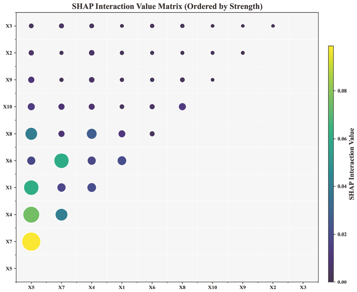
The SHAP interaction heatmap (Figure 10) can visually reflect the pairwise interaction intensity between each pair of driving factors. The results reveal that the variable combinations with the most significant interaction effects are X5 ∩ X7, X4 ∩ X5, X6 ∩ X7, X1 ∩ X5, X5 ∩ X8, and X4 ∩ X7, while the interaction intensities of the remaining variable combinations are generally weak.

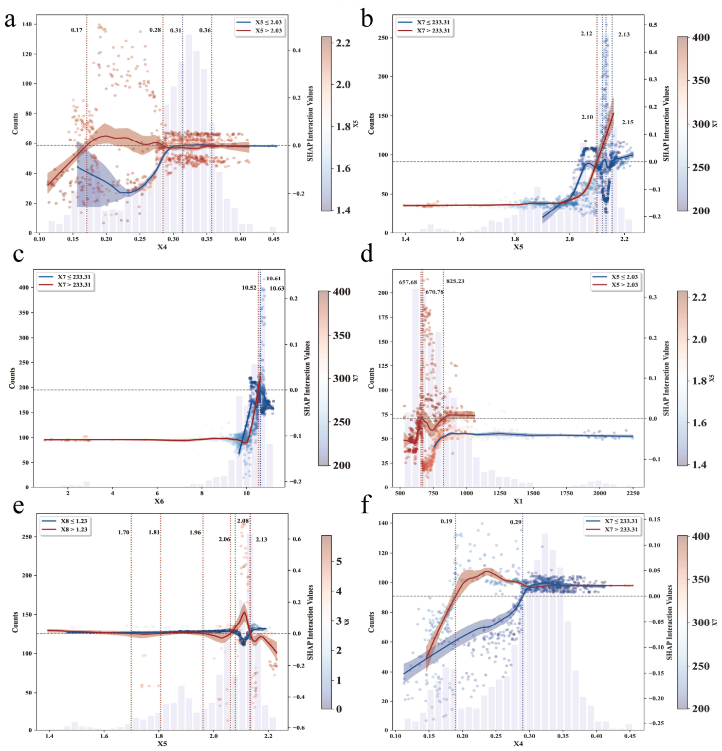
This study adopts SHAP interaction values to quantify the statistical associations between each predictive factor. To avoid subjective biases caused by relying solely on visual sorting, the top six variable combinations with the strongest interaction magnitudes were extracted, and their mean absolute SHAP interaction values were calculated. The 95% confidence intervals were constructed via 100 bootstrap resampling. Meanwhile, spatial block cross-validation datasets were utilized to test the stability of interaction magnitudes across distinct spatial partitions. Based on the above quantitative analyses, interaction plots of the six factor combinations with the highest interaction strengths were generated (Figure 11) to intuitively visualize the statistical relationships between variables.

Taking the SHAP interaction results of wind speed (X5) and precipitation (X7) (Figure 11b) as an example, X7 is observed to exert a moderating effect on the predictive process of X5. When X7 exceeds 233.31 mm, the SHAP interaction value rises continuously with the increase in X5, indicating a strong positive statistical association between the two variables, and their combined statistical signal imposes a positive influence on model outputs. By contrast, when X7 is below 233.31 mm, the SHAP interaction value only fluctuates slightly alongside X5, corresponding to weak interaction strength, and the joint association of the two variables exerts no obvious impact on model predictions.

It should be emphasized that SHAP interactions merely reflect the statistical fitting characteristics within the model and cannot directly verify the existence of real geomorphological physical coupling processes between variables. For the statistical interaction pattern between wind speed and precipitation, this paper provides reasonable geomorphological interpretations by referencing the existing literature on soil moisture content, sediment transport, vegetation coverage, and field wind erosion observations, without arbitrarily inferring causal relationships purely based on model statistical results.

4. Discussion

4.1. Morphological Characteristics of Mountain Sandy Patches

Patch area, perimeter, and shape index are core parameters for characterizing geomorphic features of sandy patches and reflecting regional landscape patterns and surface disturbance conditions, which are of great significance for revealing aeolian–geomorphic variations and ecological pattern differentiation [15]. Mountain active sandy patches in the study area exhibit obvious spatial differentiation in patch size and morphological structure, which are generally constrained by local topographic factors including elevation, slope gradient, and aspect. Statistical results show that patch area varies greatly among mountain sandy patches, and patch perimeter increases synchronously with the expansion of patch area. Shape index analysis indicates that elongated and stretched geometries dominate local sandy patches, whereas sub-circular and regular geometric patches account for a very small proportion. This reflects the unique geomorphic feature that sandy patches stretch along terrain gradients under topographic constraints of mountain slopes. Meanwhile, patch size and morphological structure vary distinctly across slope gradients, elevation zones, and aspects, highlighting the critical constraining effect of topographic setting on the spatial morphology of mountain sandy patches.

Compared with reactivated patches on fixed dunes at the southern fringe of the Tengger Desert [6], mountain active sandy patches in this study display distinctly different morphological traits. The mean major axis length of mountain sandy patches reaches 16.53 m with strong elongation. By contrast, reactivated patches in the southern Tengger Desert are dominated by small patches: over 90% of patches are less than 10 m in diameter, with an average diameter of only 5.8 m, and present highly irregular outlines. Such morphological discrepancies are mainly ascribed to the unique constraining effect of mountain slope gradient. Patch area generally tends to expand with increasing slope gradient, forming the elongated morphology that differs from flat-terrain desert landforms.

From the perspective of regional disturbance background and geomorphic context, habitat quality in the Ili River Valley continuously declined from 1980 to 2020, accompanied by substantial reduction in woodland, grassland, and cropland areas [40], which provides a macro-ecological background for the development of mountain sandy patches. Multiple human disturbances such as overgrazing and vehicle compaction are widespread across the study area, further increasing the potential probability for sandy patches to expand into larger patches. Although a small number of rodent burrows and hare traces were observed during field surveys, existing studies have confirmed that animal-derived disturbance intensity remains limited in this region and cannot exert notable influences on patch morphology and size variation [7]. Different from protective aeolian landforms such as root tube gravel veneers in the Taklamakan Desert, which can mitigate wind erosion and stabilize land surfaces [41], mountain active sandy patches represent degraded geomorphic signals caused by vegetation deterioration and intensified wind erosion disturbance. Considering geomorphic evidence, active sandy patches tend to occur on slopes and ridges subject to intensive wind erosion. Accordingly, sandy patches in our study area can be preliminarily classified as typical wind-eroded mountain sandy patches. Their morphological differentiation and spatial patterns show significant statistical associations with regional wind erosion intensity, vegetation degradation, and topographic constraints. The differentiated predictive contribution of various disturbance factors to patch morphology still requires verification by further fine-scale field monitoring.

4.2. Driving Factors of Mountain Sandy Patches

4.2.1. Interactive Statistical Characteristics of Core Predictors

SHAP interaction dependence plots (Figure 11) are adopted to interpret segmented marginal associations and threshold modulation effects of the six strongest variable pairs, with geomorphic literature cited to explain the superimposed statistical responses of multiple predictors: (a) NDVI and wind speed (X4 ∩ X5): The horizontal axis denotes NDVI values. Within the sensitive range of 0.17–0.29, SHAP interaction values rise remarkably, indicating strong positive synergies between wind and vegetation degradation. When NDVI exceeds 0.29, dense vegetation increases aerodynamic roughness and suppresses aeolian erosion, leading to weakened interactive effects. For NDVI below 0.17, the ground is fully bare with no extra superimposed responses to growing wind power, resulting in low interaction magnitudes. (b) Wind speed and precipitation (X5 ∩ X7): The horizontal axis represents near-surface wind speed. Blue dots correspond to samples with annual precipitation above 233.31 mm. Abundant runoff delivers loose erodible sediments; SHAP interaction values increase continuously with rising wind speed, jointly elevating the statistical likelihood of sandy patches. Under low precipitation (<233.31 mm), limited sediment supply restrains synergistic signals, and interaction curves fluctuate gently regardless of wind magnitude. (c) Temperature and precipitation (X6 ∩ X7): The horizontal axis shows annual mean temperature, while red dots mark samples with precipitation below 219.7 mm. High temperatures accelerate topsoil water loss under dry conditions, generating strong positive coupling that favors patch formation. Sufficient rainfall offsets thermal drought stress and diminishes interactive correlations, with fitted curves nearly overlapping the zero-effect baseline. (d) Elevation and wind speed (X1 ∩ X5): The horizontal axis stands for terrain elevation. Ridges above 645.9 m are unobstructed to valley winds, amplifying aeolian erosion and producing elevated SHAP interaction values. Valleys below this threshold are sheltered by surrounding terrain, weakening the combined statistical contribution of elevation and wind speed. (e) Wind speed and grazing intensity (X5 ∩ X8): The horizontal axis displays wind speed, and dark dots represent sites with grazing intensity over 3.60 SU/ha, which is a statistical turning point extracted from single-variable SHAP partial dependence curves. Overgrazing destroys vegetation and biological crusts, removing surface anti-wind barriers; interactive effects strengthen markedly as wind speed rises. Mild grazing retains intact ground cover and yields insignificant superimposed signals. (f) NDVI and precipitation (X4 ∩ X7): The horizontal axis is NDVI, and red dots indicate low-precipitation samples. Water scarcity confines NDVI to the sensitive interval of 0.17–0.29 and generates strong positive coupling. Adequate precipitation boosts vegetation coverage above 0.29, forming stable surface buffers and greatly reducing the interaction strength between NDVI and precipitation.

All factor pairs exhibit threshold-dependent superimposed statistical responses. No single predictor independently controls the spatial distribution of mountain sandy patches; the magnitude of marginal correlation relies on whether paired variables reach their respective critical thresholds. Such multi-factor coupling patterns collectively verify a wind–water–vegetation–grazing statistical association framework governing sandy patch occurrence in the watershed.

4.2.2. Thresholds and Synergistic Rules of Multi-Factor Interactions

To systematically disentangle the refined response patterns between mountain sandy patches and each predictive factor, this study performs a feature contribution analysis based on the XGBoost-SHAP framework. The results reveal that wind speed yields the strongest model predictive contribution among all climatic predictors to the development and evolution of mountain sandy patches. This statistical pattern aligns well with the regional geomorphic setting: mountain sandy patches are concentrated in the vicinity of wind gaps within the Ili River Valley. Under aeolian erosive forces, surfaces with damaged vegetation cover tend to develop sandy patches, which subsequently expand and coalesce. Statistically, this trend synchronizes with regional desertification expansion [42]. Aeolian sand transport capacity intensifies with rising wind speed [7]; nevertheless, surface properties (erodible/non-erodible, dry/moist) serve as critical regulators that directly modify aeolian sediment transport dynamics [9]. Therefore, mountain sandy patches exhibit greater model sensitivity to wind speed than vegetation coverage, and wind speed constitutes a core precondition for patch spatial development. Meanwhile, sandy patches represent the most dynamically responsive land units in vegetation ecosystems in terms of stability [43]. Collectively, sand patch activation arises from the combined statistical associations of multiple predictors, rather than the widespread generation of sandy patches driven by a single variable across the entire study domain.

Precipitation acts as a key predictive factor modulating mountain sandy patch dynamics by altering surface cover and hydrological conditions, thereby regulating patch expansion and vegetation rehabilitation [39]. Ecological restoration induced by precipitation increments exhibits pronounced time lags in arid zones, while minor precipitation declines rapidly correlate with desertification progression. This “slow recovery under wetting yet rapid degradation under drying” response pattern reflects the low-threshold vulnerability of arid ecosystems under reduced water availability [44], a feature also detected within this study area. When precipitation exceeds the critical threshold value, a positive statistical correlation with short-term sandy patch expansion emerges. A plausible statistical interpretation is that rainfall above this threshold predominantly generates surface runoff rather than infiltrating to replenish plant-available soil moisture; runoff transports substantial sediment to non-desert zones, which further facilitates sand patch development under subsequent aeolian processes [45]. However, this inference lacks supporting in situ hydrological and sediment monitoring data and cannot validate the underlying physical surface processes. An interpretation more consistent with the present dataset lies in the temporal mismatch between rainfall events, vegetation green-up, and topsoil moisture fluctuations. Annually composited remote sensing products fail to capture short-term soil moisture variations following discrete rainfall events, and the ecological benefits of rainfall infiltration manifest with notable delays. During the lag window before vegetation responds to water supplementation, bare sandy surfaces remain persistently exposed to wind erosion, driving continuous patch expansion. Future field hydrological monitoring is required to quantitatively partition the relative predictive contributions of runoff sediment transport and vegetation time-lag effects. Widespread precipitation scarcity characterizes arid regions of Northwest China [46], which directly shapes regional desertification severity. Previous research investigating desertification spatial patterns within the Takermohur Desert of the Ili River Valley has identified precipitation as a vital environmental predictor modulating desertification intensity [47].

Temperature accounts for merely 8.6% of the total model predictive contribution to mountain sandy patches, yet its influence cannot be overlooked despite being weaker than wind speed and precipitation. Annual mean temperatures across China’s arid zones display a distinct upward trend [48]. Warming and drying climatic conditions exhibit positive statistical associations with the spatial prevalence of mountain sandy patches within the study dataset. In terms of topographic predictors, elevations above 645.90 m exhibit positive statistical associations with mountain sandy patches, and the magnitude of this correlation rises nonlinearly with increasing elevation. Slope gradient shows distinct statistical correlations with mountain sandy patch occurrence. Within the dataset, steeper terrain coincides with higher runoff loss and lower topsoil moisture, which corresponds to an elevated statistical likelihood of mountain sandy patches [6]. Among anthropogenic predictive factors, grazing intensity delivers the highest model predictive contribution to mountain sandy patches, and distinct threshold response patterns exist between the two variables. Under low grazing intensity, SHAP values are predominantly positive, indicating no pronounced adverse statistical linkage between mild grazing and sandy patch occurrence. By contrast, sustained grazing intensification correlates with progressive sand patch development. Surface roughness is jointly modulated by aridity levels and grazing pressure [49]. Long-term overgrazing drastically reduces surface roughness length, enabling wind energy to directly interact with sandy grassland surfaces and indirectly raising the statistical likelihood of mountain sandy patch emergence [50]. Nighttime light intensity and population distribution contribute 2.2% and 2.7% to total model predictive importance, respectively; as anthropogenic disturbance intensity increases, the statistical correlation strength between natural predictors and desertification gradually attenuates [51].

In summary, grazing intensity constitutes the anthropogenic predictor with the highest predictive contribution to mountain sandy patches. Nighttime light and population exhibit low overall contribution magnitudes and are not core predictive variables, yet their positive statistical associations with sand patches continuously strengthen once each exceeds its respective threshold. This pattern is tied to the study area’s geographic location: the research sites are situated on the ridgelines of the Keguqin Mountains, approximately 30 km from the county seat, resulting in generally weak direct human disturbance across the watershed. Even so, their statistical linkages with mountain sandy patches remain worthy of consideration.

4.3. Limitations and Future Perspectives

It must be emphasized that this cross-sectional snapshot dataset only captures static spatial statistical correlations at a single time point and cannot identify temporal causal sequences or sequential geomorphic processes such as wind erosion initiation, soil moisture limitation, and grazing disturbance succession. All identified thresholds and association patterns are dataset-specific conceptual hypotheses requiring long-term multi-temporal field monitoring for further validation. The four sampling plots were selected via accessibility-stratified sampling rather than fully random sampling, leading to potential selection bias; the statistical patterns derived cannot be arbitrarily generalized to all mountain watersheds with distinct terrain and grazing regimes.

Based on UAV data, multi-source remote sensing datasets, and the interpretable machine learning framework of XGBoost-SHAP, this study systematically analyzes the morphological characteristics and driving factors of mountain sandy patches in the Sarbulak River Basin. It fills the research gaps regarding the morphological features and driving mechanisms of mountain sandy patches, and reveals the static spatial association pattern of patch distribution of mountain sandy patches in the study area characterized by “wind erosion dominance, precipitation regulation, grazing intensification and vegetation suppression” from the two dimensions of morphology and driving forces. The research findings can provide a scientific basis for ecological management and sustainable restoration of similar degraded patches in the Sarbulak River Basin and the Ili River Valley. Nevertheless, several limitations remain in this study. First, key covariates including soil texture, topsoil moisture, biological soil crusts, lithology, extreme wind events, seasonal snow cover, shallow groundwater, and historical fire records were not incorporated into the model, leading to evident omitted variable bias. Soil texture, lithology, and biological crusts jointly determine regional sediment supply and the baseline wind erosion resistance of land surfaces. As intermediate regulating factors linking precipitation and aeolian erosion, soil moisture, snow cover, and groundwater can substantially alter the stage-specific erodibility of topsoil. Extreme wind events and historical wildfires act as short-term intense disturbances that rapidly reshape surface cover and sediment transport conditions. This study only constructs the predictive model based on annual average climatic indices and macroscopic topographic metrics, and thus cannot isolate the potential confounding effects of the above missing variables. Uncertainties exist in the marginal association strength, interactive statistical characteristics, and response thresholds of all relevant predictive factors. The derived conclusions merely reflect statistical correlations within the current variable framework, and fail to capture heterogeneous geomorphological responses induced by extreme climatic conditions and inherent soil properties. The statistical thresholds obtained herein can only serve as preliminary references for watershed desertification research. Second, the selected field sample plots cover limited spatial extents, which cannot fully represent the overall spatial patterns of mountain active sandy patches. Meanwhile, the multi-source remote sensing datasets adopted in this work possess relatively coarse spatial resolution, restricting fine-scale analysis of the spatiotemporal dynamics of sandy patch distribution. Third, although the SHAP framework enhances model interpretability by quantifying the directional marginal association and relative predictive importance of each variable, this method cannot disentangle complex causal linkages between predictors or resolve the intrinsic processes of aeolian geomorphology and ecosystem evolution. Fourth, mountain active sandy patch boundaries were extracted through manual visual digitization. Standardized interpretation protocols and double-person cross-verification were implemented during mapping, yet positional uncertainty still persists for vector boundaries. Minor positional deviations will trigger error propagation and reduce the estimation precision of morphological metrics including patch area, perimeter, surface area, and volume. Corresponding improvements can be made in future research to address the above deficiencies. First, integrate high-resolution remote sensing data supplemented by field measured verification to improve the accuracy of characterizing patch occurrence mechanisms. Second, expand sampling plot coverage to obtain more morphological parameters and clarify the refined morphological traits of mountain sand activation. Restricted by research duration and field conditions, this paper only preliminarily explores the morphology and driving factors of mountain sandy patches. Many critical issues remain to be further investigated, including the ecological impacts induced by the progressive development of mountain sandy patches, sedimentary environments of sandy patches, and their spatiotemporal distribution patterns.

5. Conclusions

This study adopts UAV high-precision topographic data and the XGBoost-SHAP interpretive machine learning framework to explore the static spatial statistical relationships between mountain sandy patches and environmental predictors within the Sarbulak River Basin. Rather than reiterating detailed morphological metrics and predictor threshold statistics presented in the Abstract and Results (Section 3), this section emphasizes research limitations, follow-up monitoring schemes, and the applicable boundary of our quantitative statistical outputs.

First, prominent uncertainties exist within the current analytical framework. The dataset only contains single-period UAV cross-sectional observations captured in October 2024, which cannot capture sequential temporal geomorphic processes or distinguish causal sequences between environmental variables and sandy patch distribution. The four sampling plots were selected via accessibility-based stratified sampling instead of full random sampling, leading to inherent selection bias; the statistical thresholds and correlation patterns extracted from this dataset cannot be arbitrarily extrapolated to mountain watersheds with divergent terrain, grazing intensity, and climate backgrounds. In addition, several critical covariates including soil texture, biological crust coverage, near-surface soil moisture, and seasonal snow cover were not incorporated into the model, which inevitably introduces omitted variable bias and restricts the robustness of model outputs. Coarse 1 km original climate grids resampled to 250 m also create widespread spatial pseudo-replication across patch samples, further increasing uncertainty in SHAP-based predictive importance rankings. Moreover, SHAP outputs only reflect statistical covariation within the established model and cannot verify real physical coupling mechanisms among geomorphic factors. Second, targeted multi-temporal field monitoring is proposed for follow-up research to offset the above deficiencies. Future work will integrate annual repeated UAV surveys, in situ soil moisture, and wind erosion field measurements, and seasonal grazing tracking data to build long-term time-series datasets. Field sampling coverage will be expanded to cover more elevation and slope gradients across the whole basin with random transect layout, reducing sampling representativeness defects. Supplementary soil sediment and biological crust surveys will also be conducted to enrich environmental predictor systems and weaken omitted variable interference. Third, clear applicable boundaries must be clarified when applying the quantitative thresholds identified in this work to local ecological governance. All critical statistical intervals derived from SHAP dependence curves are dataset-specific reference values under the 2018–2023 multi-year average climate background of the Sarbulak River Basin, rather than universal rigid regulatory standards. When utilizing these thresholds for grazing adjustment and aeolian degradation risk warning, managers need to combine real-time annual climate fluctuations, seasonal vegetation variations, and local microtopographic conditions for comprehensive judgment. For watersheds with distinct substrate, wind field, and grazing regimes, repeated field surveys and localized model calibration are required before referencing the quantitative indicators proposed in this paper.

References

1. Zhu, Z.D. Concept, Cause and Control of Desertification in China. Quat. Sci. 1998, 18, 145–155. [Google Scholar]
2. Zhu, Z.D. Fragile Ecological Zones and Land Desertification in China. J. Desert Res. 1991, 11, 11. [Google Scholar]
3. Zhou, R.P. Zonation and Spatiotemporal Evolution of China’s Desertification. J. Geo-Inf. Sci. 2019, 21, 675–687. [Google Scholar]
4. Sun, Y.; Du, H.S.; Liu, M.P.; Hasi, E. Research Progress on Morphodynamics of Blowouts. Sci. Geogr. Sin. 2015, 35, 898–905. [Google Scholar]
5. Yu, Y.J.; Yu, Z.Y.; Lu, C.X. Preliminary Study on Activated Sand Patches in Artificial Vegetation Area of Shapotou. J. Desert Res. 1998, 18, 87–90. [Google Scholar]
6. Wu, Y.Z.; Lin, Q.G.; Huang, L.; Zhao, Y.; Zhang, Z.S. Spatial Distribution Characteristics of Activated Sand Patches on the Southern Margin of the Tengger Desert. J. Lanzhou Univ. (Nat. Sci.) 2018, 54, 776–782. [Google Scholar]
7. Dun, Y.-Q.; Qu, J.-J.; Kang, W.-Y.; Li, M.-L.; Liu, B.; Wang, T.; Shao, M. Formation and ecological response of sand patches in the protection system of Shapotou section of the Baotou-Lanzhou railway, China. J. Arid Land 2024, 16, 298–313. [Google Scholar] [CrossRef] [Scilit]
8. Levin, S.A. The Problem of Pattern and Scale in Ecology. Ecology 1992, 73, 1943–1967. [Google Scholar] [CrossRef] [Scilit]
9. Delorme, P.; Nield, J.M.; Wiggs, G.F.S.; Baddock, M.C.; Bristow, N.R.; Best, J.L.; Christensen, K.T.; Claudin, P. Field Evidence for the Initiation of Isolated Aeolian Sand Patches. Geophys. Res. Lett. 2023, 50, e2022GL101553. [Google Scholar] [CrossRef] [Scilit]
10. Lancaster, N. Field Studies of Sand Patch Initiation Processes on the Northern Margin of the Namib Sand Sea. Earth Surf. Process. Landf. 1996, 21, 947–954. [Google Scholar] [CrossRef]
11. Lopuch, M.; Sokołowski, R.J.; Jary, Z. Factors Controlling the Development of Cold-Climate Dune Fields within the Central Part of the European Sand Belt—Insights from Morphometry. Geomorphology 2023, 420, 108514. [Google Scholar] [CrossRef] [Scilit]
12. Larson, E.J.L. Topographic Effects on Titan’s Dune-Forming Winds. Atmosphere 2019, 10, 600. [Google Scholar] [CrossRef] [Scilit]
13. Cossitt, R.R. Aeolian Processes in the Seward Sand Hills, Saskatchewan, Canada; University of Regina: Regina, SK, Canada, 2002. [Google Scholar]
14. Kilibarda, Z.; Kilibarda, V. Seasonal Geomorphic Processes and Rates of Sand Movement at Mount Baldy Dune in Indiana, USA. Aeolian Res. 2016, 23, 103–114. [Google Scholar] [CrossRef] [Scilit]
15. Li, B.; Zhang, J.T. Index and Fractal Analysis of Grassland Landscape Patch Shape on the Loess Plateau. Acta Agrestia Sin. 2010, 18, 141–147. [Google Scholar]
16. Visser, N.; Botha, J.C.; Hardy, M.B. Re-Establishing Vegetation on Bare Patches in the Nama Karoo, South Africa. J. Arid. Environ. 2004, 57, 155–177. [Google Scholar] [CrossRef] [Scilit]
17. Sevink, J.; Wallinga, J.; Reimann, T.; van Geel, B.; Brinkkemper, O.; Jansen, B.; Romar, M.; Bakels, C. A Multi-Staged Drift Sand Geo-Archive from the Netherlands: New Evidence for the Impact of Prehistoric Land Use on the Geomorphic Stability, Soils, and Vegetation of Aeolian Sand Landscapes. Catena 2023, 224, 106969. [Google Scholar] [CrossRef] [Scilit]
18. Wei, X.; Li, S.; Yang, P.; Cheng, H. Soil Erosion and Vegetation Succession in Alpine Kobresia Steppe Meadow Caused by Plateau Pika—A Case Study of Nagqu County, Tibet. Chin. Geogr. Sci. 2007, 17, 75–81. [Google Scholar] [CrossRef] [Scilit]
19. Song, M.-H.; Cornelissen, J.H.C.; Li, Y.-K.; Xu, X.-L.; Zhou, H.-K.; Cui, X.-Y.; Wang, Y.-F.; Xu, R.-Y.; Feng, Q. Small-Scale Switch in Cover–Perimeter Relationships of Patches Indicates Shift of Dominant Species during Grassland Degradation. J. Plant Ecol. 2020, 13, 704–712. [Google Scholar] [CrossRef] [Scilit]
20. Fu, T.; Li, X. Evaluating the Stability of Artificial Sand-Binding Vegetation by Combining Statistical Methods and a Neural Network Model. Sci. Rep. 2023, 13, 6544. [Google Scholar] [CrossRef] [Scilit] [PubMed]
21. Zhang, J.; Liu, D.; Meng, B.; Chen, J.; Wang, X.; Jiang, H.; Yu, Y.; Yi, S. Using UAVs to Assess the Relationship between Alpine Meadow Bare Patches and Disturbance by Pikas in the Source Region of Yellow River on the Qinghai-Tibetan Plateau. Glob. Ecol. Conserv. 2021, 26, e01517. [Google Scholar] [CrossRef] [Scilit]
22. Sloey, T.M.; Willis, J.M.; Hester, M.W. Hydrologic and Edaphic Constraints on Schoenoplectus acutus, Schoenoplectus californicus, and Typha latifolia in Tidal Marsh Restoration. Restor. Ecol. 2015, 23, 430–438. [Google Scholar] [CrossRef] [Scilit]
23. Yao, X.; Wang, H.; Zhang, S.; Oosthuizen, M.; Huang, Y.; Wei, W. Impact of Plateau Pika Burrowing Activity on the Grass/Sedge Ratio in Alpine Sedge Meadows in China. Front. Plant Sci. 2022, 13, 1036438. [Google Scholar] [CrossRef] [Scilit] [PubMed]
24. Xia, C.X. Remote Sensing Dynamic Analysis of Land Desertification in Western Jilin Province. Master’s Thesis, Jilin University, Changchun, China, 2017. [Google Scholar]
25. Sun, T.; Wang, J.-H.; Liu, H.-J.; Ji, Y.-F.; Ding, F.; Yuan, H.-B. Analysis on Vegetation Characteristics of Activating Sand Dunes in the Oasis–Desert Ecotone. Res. Soil Water Conserv. 2009, 16, 174–178. [Google Scholar]
26. De Freitas, E.M.; Trevisan, R.; Schneider, Â.A.; Boldrini, I.I. Floristic Diversity in Areas of Sandy Soil Grasslands in Southwestern Rio Grande do Sul, Brazil. Rev. Bras. Biociênc. 2010, 8, 112. [Google Scholar]
27. Meng, T.T.; Ni, J.; Wang, G.H. Plant Functional Traits: Linkages with Environment and Ecosystem Function. J. Plant Ecol. 2007, 1, 150–165. [Google Scholar] [CrossRef] [Scilit]
28. Zhou, Y.; Hasi, E.; Wang, Z.; Qing, D.; Han, X.; Yin, J.; Wu, Z. Dynamics of Blowouts Indicating the Process of Grassland Desertification. Land Degrad. Dev. 2022, 33, 2885–2897. [Google Scholar] [CrossRef] [Scilit]
29. Bao, Z.X.; Wang, J.; Zhang, X.W. Spatial Differentiation of Blowouts and Their Vegetation Constraints in Hulunbuir Sandy Grassland. Arid. Zone Res. 2024, 41, 1422–1432. [Google Scholar]
30. Feng, R.; Aimaiti, A. Discussion on the Changes of Material Life and Folk Culture of Kazakh People in Xinjiang—A Case Survey of Sarbulak Township, Huocheng County, Ili. J. Northwest Minzu Univ. (Philos. Soc. Sci.) 2008, 3, 110–118. [Google Scholar]
31. Wang, P.; Ma, Q.; Zhu, Y.P. Grain Size Characteristics of Surface Sediments of Nebkhas on the Northern Margin of the Takermohur Desert, Xinjiang. J. Gansu Agric. Univ. 2021, 44, 1644–1653. [Google Scholar]
32. Li, X.B. Discussion on Large-Scale Enclosure for Sand Fixation, Forest and Grass Cultivation. Xinjiang Agric. Sci. Technol. 1987, 1, 44–45. [Google Scholar]
33. Wu, Y.Z.; Shi, K.F.; Chen, Z.Q.; Liu, S.R.; Chang, Z.J. An Improved Time-Series DMSP-OLS-Like Data (1992–2023) in China by Integrating DMSP-OLS and SNPP-VIIRS; Harvard Dataverse, V5. IEEE Trans. Geosci. Remote Sens. 2021, 60, 1–14. [Google Scholar] [CrossRef]
34. Kong, X.; Lai, F.B.; Chen, S.J.; Zhu, X. Morphological Characteristics and Spatial Pattern of Populus Euphratica Dune and Vortex Dune in Bilikum Desert. J. Sediment Res. 2020, 45, 59–65. [Google Scholar]
35. Liu, R.H.; Jiang, Y.; Chang, B.; Li, J.; Rong, C.; Liang, S.; Yang, R.; Liu, X.; Zeng, H.; Su, X.; et al. Interspecific Association and Correlation Analysis of Main Woody Plants of Pterocarya stenoptera Community in Lijiang River Riparian Zone. Acta Ecol. Sin. 2018, 38, 6881–6893. [Google Scholar] [CrossRef] [Scilit]
36. Bentéjac, C.; Csörgő, A.; Martínez-Muñoz, G. A Comparative Analysis of XGBoost. arXiv 2019, arXiv:1911.01914. [Google Scholar]
37. Fatima, S.; Hussain, A.; Amir, S.B.; Ahmed, S.H.; Aslam, S.M.H. XGBoost and Random Forest Algorithms: An in Depth Analysis. Pak. J. Sci. Res. 2023, 3, 26–31. [Google Scholar] [CrossRef] [Scilit]
38. Sun, D.L.; Wu, X.Q.; Wen, H.J.; Ma, X.L.; Zhang, F.T.; Ji, Q.; Zhang, J.L. Ecological Security Pattern Based on XGBoost-MCR Model: A Case Study of the Three Gorges Reservoir Region. J. Clean. Prod. 2024, 470, 143252. [Google Scholar] [CrossRef] [Scilit]
39. Van den Broeck, G.; Lykov, A.; Schleich, M.; Suciu, D. On the Tractability of SHAP Explanations. J. Artif. Intell. Res. 2022, 74, 851–886. [Google Scholar] [CrossRef] [Scilit]
40. Sui, L.; Yan, Z.M.; Li, K.F.; He, P.E.; Ma, Y.J.; Zhang, R.C. Prediction of Habitat Quality under the Influence of Human Activities and Climate Change in Ili River Valley. Arid. Land Geogr. 2024, 47, 104–116. [Google Scholar]
41. Luo, H.Y.; Lai, F.B.; Chen, S.J.; Zhu, X. Morphology and Distribution of Root Canal Gravel Curtain in Bilikum Desert, Taklamakan. J. Desert Res. 2019, 39, 200–208. [Google Scholar]
42. Li, X.R. Effects of Spatial Heterogeneity of Soil on Vegetation Restoration in Arid Sandy Regions. Sci. China Ser. D Earth Sci. 2005, 35, 361–370. [Google Scholar]
43. Huang, L.; Zhang, Z. The Stability of Revegetated Ecosystems in Sandy Areas: An Assessment and Prediction Index. Water 2015, 7, 1969–1990. [Google Scholar] [CrossRef] [Scilit]
44. Wei, W.S. Response and Feedback of Modern Deserts to Climate Change: A Case of Gurbantünggüt Desert. Chin. Sci. Bull. 2000, 45, 636–641. [Google Scholar]
45. Hua, T.; Wang, X.M. Research Progress on Mutual Feedback between Desertification and Climate Change in Arid and Semi-Arid Regions of East Asia. Prog. Geogr. 2014, 33, 841–852. [Google Scholar]
46. Liu, Y.Y.; Zhang, X.Q.; Sun, Y. Spatiotemporal Variation Characteristics of Precipitation in Rainy Season in Arid Northwest China under Global Warming. Adv. Clim. Change Res. 2011, 7, 97–103. [Google Scholar]
47. Song, Y.; Lai, F.B.; Huang, K.L.; Zhuang, X.P.; Zubaidai, W.A. Spatiotemporal Pattern Evolution and Influencing Factors of Desertified Land in Takermohur Desert over the Past 30 Years. Acta Sci. Nat. Univ. Sunyatseni 2025, 64, 149–159. [Google Scholar]
48. Zhang, X.Q.; Sun, Y.; Mao, W.Y.; Liu, Y.Y.; Ren, Y. Regional Response of Temperature Change to Global Warming in Arid Areas of China. Arid. Zone Res. 2010, 27, 592–599. [Google Scholar]
49. Sun, J.; Hou, G.; Liu, M.; Fu, G.; Zhan, T.; Zhou, H.; Tsunekawa, A.; Haregeweyn, N. Effects of Climatic and Grazing Changes on Desertification of Alpine Grasslands, Northern Tibet. Ecol. Indic. 2019, 107, 105647. [Google Scholar] [CrossRef] [Scilit]
50. Li, S.G.; Harazono, Y.; Oikawa, T.; Zhao, H.L.; He, Z.Y.; Chang, X.L. Grassland Desertification by Grazing and the Resulting Micrometeorological Changes in Inner Mongolia. Agric. For. Meteorol. 2000, 102, 125–137. [Google Scholar] [CrossRef] [Scilit]
51. Guo, B.; Wei, C.; Yu, Y.; Liu, Y.; Li, J.; Meng, C.; Cai, Y. The Dominant Influencing Factors of Desertification Changes in the Source Region of Yellow River: Climate Change or Human Activity? Sci. Total Environ. 2022, 813, 152512. [Google Scholar] [CrossRef] [Scilit] [PubMed]
Figure 1. Map of the study area: (a) elevation of the Ili River Valley; (b) study area and sampling plots; (c) oblique aerial photograph of mountain sandy patches; and (d) orthophoto of mountain sandy patches.
Sustainability 18 08649 g001
Figure 2. Spatial distribution of driving factors in the study area.
Sustainability 18 08649 g002
Figure 3. (a) Residual spatial scatter plot: The horizontal and vertical axes (X, Y) represent the geographic coordinates of sampling points. The color of each point denotes the residual value (observed value − predicted value) of the training sample at that location. (b) Empirical variogram of training residuals: Numerous light-colored dots illustrate the relationship between semivariance (half of the squared residual difference between two points) and geographic distance calculated for all pairs of sampling points. The red line represents the binned average semivariance, which reflects the overall trend. The blue dashed line denotes the variance of overall residuals (Sill) and serves as a reference line. Model comparison metrics were calculated under an identical leave-one-plot 5-fold spatial cross-validation framework.
Sustainability 18 08649 g003
Figure 4. Histogram and boxplot of major axis lengths for 92 mountain sandy patches. The upper subplot shows the frequency histogram of sandy-patch major-axis length. The lower subplot is a box-whisker plot, where the box covers the interquartile range (IQR, 25th–75th percentiles), the internal solid line represents the median, whiskers reach 1.5 × IQR, and orange dots denote outlier observations. N = 92 indicates the total number of sandy-patch samples.
Sustainability 18 08649 g004
Figure 5. Morphological characteristics and perimeter grading of mountain sandy patches across 8 grouped sampling plots (1 = Plot 1, 2–4 = Plot 2, 5–6 = Plot 3, and 7–8 = Plot 4). Contour lines with different colors represent the patch perimeter (C, unit: m): 2–11 (grey), 11–21 (orange), 21–30 (yellow), 30–43 (light green), 43–60 (blue), 60–80 (purple), 80–108 (pink), and 108–240 (red). The scale bar represents the horizontal distance in meters.
Sustainability 18 08649 g005
Figure 6. Overfitting diagnostic plots for the XGBoost regression model: (a) Scatter plot of observed versus predicted values for the XGBoost regression model. Blue circles = training set (n = 930); red triangles = test set (n = 310); and black dashed line = 1:1 perfect fitting line (y = x). Model evaluation metrics are annotated in the lower-right box: training set (R2 = 0.9507), RMSE = 0.3066; test set (R2 = 0.8537), RMSE = 0.5879. The model was built with a 7:3 train–test split and validated via 5-fold spatial block cross-validation combined with grid search hyperparameter tuning. (b) Learning curves of the XGBoost regression model. The curves illustrate the variation in RMSE for the training set and validation set with increasing training iterations, which is used to diagnose model overfitting. (c) Residual scatter plot of the XGBoost regression model. Residual values (observed value minus predicted value) are plotted against observed values to reveal systematic prediction bias. Orange dots are residual observations and the black dashed line marks the zero-residual baseline. (d) Histogram of prediction errors derived from leave-one-plot-out 5-fold spatial cross-validation, reflecting the overall fluctuation range of model prediction error.
Sustainability 18 08649 g006
Figure 7. Heatmap of correlations among driving factors: Circle size denotes absolute correlation magnitude; color gradient from blue (negative correlation) to red (positive correlation). Significance levels: *** p < 0.001, * p < 0.05, and ns = non-significant (p ≥ 0.05). X1 = elevation; X2 = aspect; X3 = slope; X4 = NDVI; X5 = wind speed; X6 = temperature; X7 = precipitation; X8 = grazing intensity; X9 = nighttime light; and X10 = population distribution.
Sustainability 18 08649 g007
Figure 8. (a) Summary plot of driving factor importance; (b) SHAP summary dot plot: the horizontal position of each dot represents the SHAP value; the vertical axis denotes different driving variables. The gradient from blue to red indicates low to high feature values. Points distributed on the right side of the horizontal zero line mean that the corresponding variable facilitates the development of sandy patches, while points on the left side indicate an inhibitory effect. X1 = elevation; X2 = aspect; X3 = slope; X4 = NDVI; X5 = wind speed; X6 = temperature; X7 = precipitation; X8 = grazing intensity; X9 = nighttime light; and X10 = population distribution.
Sustainability 18 08649 g008
Figure 9. SHAP dependence plots illustrating the nonlinear responses of mountain sandy patches to each individual predictive factor (subgraphs (aj) correspond to X1–X10 sequentially). The colored scattered dots denote individual sample observations (red for positive SHAP values, blue for negative SHAP values). The solid black line refers to the LOWESS locally weighted smoothing trend line, and the grey shaded band represents the 95% confidence interval calculated via 100 bootstrap resampling. The horizontal dashed line is the reference line at SHAP = 0, while vertical dotted lines mark the median thresholds (statistical inflection thresholds) of effect transitions extracted from the dataset. Green shaded areas indicate intervals of positive marginal association, and pink shaded areas represent intervals of negative marginal association. Variable definitions: X1 = elevation, X2 = aspect, X3 = slope, X4 = Normalized Difference Vegetation Index (NDVI), X5 = wind speed, X6 = temperature, X7 = precipitation, X8 = grazing intensity, X9 = nighttime light, and X10 = population distribution.
Sustainability 18 08649 g009
Figure 10. SHAP interaction value matrix of pairwise driving factor combinations, ordered by interaction strength. Dot color gradient from dark purple (low interaction value) to bright yellow (maximum interaction value). Horizontal and vertical axes represent the ten driving factors X1–X10. The color bar on the right quantifies the magnitude of SHAP interaction values. X1 = elevation; X2 = aspect; X3 = slope; X4 = NDVI; X5 = wind speed; X6 = temperature; X7 = precipitation; X8 = grazing intensity; X9 = nighttime light; and X10 = population distribution.
Sustainability 18 08649 g010
Figure 11. SHAP interaction dependence plots for six key factor pairs. Subplots: (a) NDVI–wind speed; (b) wind speed–precipitation; (c) temperature–precipitation; (d) elevation–wind speed; (e) wind speed–grazing intensity; and (f) NDVI–precipitation. Dot color denotes the magnitude of the paired variable. Black solid lines represent fitted SHAP interaction curves. Vertical dashed lines indicate statistically derived thresholds. Background histograms show sample distribution along the x-axis. Legends denote 95% bootstrap confidence intervals. SHAP interaction values > 0 indicate positive statistical contribution to sandy patch occurrence, whereas values < 0 indicate inhibitory effects. Note that SHAP interactions reflect statistical model-fitting patterns rather than proven geomorphological causal coupling. The horizontal dashed lines denote reference baselines. Colored shaded regions correspond to confidence intervals of fitted curves. Vertical dashed lines mark critical threshold values, and scattered dots represent individual sample observations.
Sustainability 18 08649 g011