Green-AI-Aware Smart Grid Stability Prediction Using Hybrid CNN, Random Forest, and XGBoost Fusion

Abstract

The increasing integration of renewable energy sources and smart grid (SG) technologies introduces significant challenges to power system stability due to the inherent variability and uncertainty of electricity generation and demand. While many machine learning and deep learning approaches have been proposed for stability prediction, various studies focus only on predictive performance and offer limited assessment of computational efficiency, statistical significance, and sustainability-related metrics. To address these gaps, this study suggests a hybrid fusion approach that combines Convolutional Neural Networks (CNNs), eXtreme Gradient Boosting (XGBoost), and Random Forest (RF) classifiers through a soft voting strategy for SG stability prediction. The CNN component automatically extracts representative features, while XGBoost and RF contribute complementary classification capabilities, reducing the need for manual feature engineering. In addition to predictive evaluation, a Green AI-oriented benchmarking framework is introduced to evaluate model performance using predictive accuracy, computational runtime, memory consumption, and estimated computational CO₂ emissions associated with model training and inference. The proposed framework is assessed on the UCI SG Stability dataset using stratified cross-validation and statistical significance testing, including Friedman and Nemenyi post hoc analyses. Experimental results demonstrate that the fusion model achieves 97.68% classification accuracy and an AUC of 0.991, exceeding several individual machine learning, deep learning, and ensemble baselines. Statistical analysis shows significant improvements over recurrent deep learning models such as LSTM and GRU. However, the differences from strong tree-based methods, including XGBoost and RF, are not statistically significant. Furthermore, the proposed model reaches a high sustainability score of 0.802, indicating a favorable balance between predictive performance and computational resource requirements. The findings show that the proposed framework is effective and computationally efficient to predict the stability of the smart grid on the UCI benchmark dataset and also serves as a transparent green AI benchmarking methodology for comparative studies in the future. The validation of the approach on real-world smart grid data under noisy, not fully complete, and heterogeneous operating conditions is another interesting research direction for future work.

1. Introduction

The significant technological development, combined with the current shift to smart cities around the world, has greatly raised the need to change the design of contemporary power systems. Conventional electrical systems were built on the traditional centralized generation model, in which generation is carried out in large plants and then transmitted over long distances to the final consumers [1]. These traditional systems are based on a unidirectional flow of power and communication that is insufficient to deal with the dynamic and complex energy needs of modern societies [2,3]. Reaching a balance in electricity supply and demand with reliability, at a lower cost, and without interruption is a basic issue in the operation of power systems. Grid stability occurs when the generated power is equal to consumption in real time, thus keeping the system frequency within acceptable limits. The increasing use of renewable energy sources, however, has introduced more complex problems in achieving grid stability. Recently, renewable energy technologies like solar, wind, and hydropower are being widely adopted, as decarbonization strategies to curb greenhouse gas emissions are being widely pursued in many countries. Although these sources contribute to more sustainability and energy security, their intermittency and variability pose a major challenge to grid management [4].

In response to these challenges, new power systems are developing into smart grid (SG) architectures. SGs use sophisticated sensing, communication, and control technology to facilitate two-way flow of energy and real-time measurement. These systems increase operational efficiency, minimize transmission losses, and enhance reliability by incorporating distributed energy resources and actively involving consumers. Smart sensors and intelligent monitoring systems can be deployed, and early fault detection and more responsive grid management are possible, which can significantly enhance the overall performance and reliability of SGs. The Decentral SG Control (DSGC) framework is one of the most researched methods of stabilizing SGs, as it uses grid frequency as a signal to stabilize demand and supply. In this regard, the higher the frequency, the more generation is in excess, and vice versa. Despite giving a mathematical perspective to the analysis of grid dynamics, DSGC is based on oversimplified assumptions and constant input parameters, which can restrict its usefulness in practice, particularly in real-world scenarios where grid conditions are variable and unpredictable. Moreover, the concerns of scalability, adaptability, and equity of distributed participants are also of great concern [5].

Considering these constraints, the interest in using data-driven methods, especially machine learning (ML) or deep learning (DL), to improve grid stability analysis and prediction is increasing. The capabilities of ML and DL models include the ability to learn about complex nonlinear relationships, evolve to changing conditions of the system, and handle large-scale data produced by the infrastructure of SGs. With the combination of the new learning algorithms with the old models of power systems, one can come up with more robust, accurate, and flexible solutions to stability assessment, which can lead to improved decision-making and enhanced reliability of SG operations [6].

1.1. Existing Systems

The transformation of traditional power grids into SGs signifies considerable progress in improving efficiency and sustainability in the energy sector. However, the integration of renewable energy sources and the complex network of networked devices has initiated additional challenges, particularly with grid stability, such as fluctuations in energy supply and demand that can produce power cuts or inefficiencies. Providing and upholding grid stability guarantees an uninterrupted electricity supply and averts possible disruptions. Many recent research projects focus on building a smart system based on ML techniques to detect and predict SG stability. In [7], Mohsen et al. presented an artificial neural network (ANN) to predict the stability of SGs for decentralized SG control (DSGC) systems. This neural network was used on a dataset built from simulations of grid stability conducted on a four-node network with a star topology, focusing on two categories of grid stability: stable and unstable. The Keras framework was employed to train the suggested neural network, and a hyperparameter optimization technique was implemented to attain high accuracy. Titz et al. proposed in [8] an integration of network science measurements and ML models to forecast the danger of desynchronization events. Network science offers measurements for critical characteristics of transmission lines, like redundancy and centrality. ML methods inherently pick features, thereby identifying critical elements that influence network robustness and vulnerability. They used simulated data from various synthetic test grids to train and evaluate these models.

In [9], Alsirhani et al. proposed a smart and available grid prediction system integrated with reliable mechanisms to meet the fluctuating energy demands. The engagement of consumers and producers was one of the many elements that may impact the grid’s stability. Alsirhani and his co-authors suggested a novel system for detecting stability statistics in SG systems based on a multi-layer perceptron–extreme learning machine (MLP-ELM) technique. Additionally, the principal component analysis (PCA) technique was used for extracting features. The authors in [10] proposed five distinct cascade methodologies for assessing the stability of SG systems and classifying the different SG stability types. In the preprocessing step, the SG dataset undergoes feature selection based on Relief, Correlation filtering technique, and a supervised attribute filter. After that, they applied the resampling method followed by Fuzzy C-Means Clustering-Based Feature Weighting (FCMFW). After that, three methodologies were applied before the classification algorithm: 5-fold cross-validation, 10-fold cross-validation, and hold-out (50–50%). Finally, five distinct classification algorithms were used to classify the SG dataset.

Allal et al. in [11] investigated the stability of the SG based on ML techniques. The authors framed the issue as a binary classification task by considering two possibilities (stable or unstable grid). They also attempted to estimate continuous values showing grid stability levels. These values were used later to predict grid stability based on a predetermined threshold. To handle data imbalance, the Synthetic Minority Over-sampling Technique (SMOTE) and K-means SMOTE were utilized. The investigation includes many regressors and classifiers, including tree-based models, boosting techniques, ensemble methods, and multi-layer perceptrons (MLPs). In [12], the authors proposed a method for enhancing the stability prediction of Internet of Things (IoT)-driven SGs using various ML models, such as Gradient Boosting (GB), K-Nearest Neighbor (KNN), Support Vector Machine (SVM), neural networks, and the decision tree classifier. They also investigated the efficacy of hyperparameter-optimized GB models in forecasting SG dynamic stability, which indicates the system’s ability to revert to a stable operating point after a disruption.

Ghazal et al. [13] suggested the development of an explainable hybrid forecasting model using Explainable AI and deep learning for predicting the stability of a four-node smart grid. The integration of accurate predictions and explainability made it possible to forecast the stability of the grid and detect component failure and poor power distribution. Nonetheless, the research did not take into account computational efficiency, memory usage, execution time, and carbon emissions. This highlights the need to use carbon-aware AI platforms that evaluate both prediction and carbon footprint simultaneously.

1.2. Gaps of Existing Models

Even recently, the detection of SG stability has received significant attention from researchers and industry, but many gaps still exist, as illustrated in

Table 1. Summary of the main gaps in existing work on SG stability prediction and the models used.

Ref	Key Techniques Used	Main Gaps
Mohsen [7]	ANN, Keras, hyperparameter tuning	Based on simple ANN (without deep/temporal modeling) Trained on simplified simulated grid data Focus only on binary stability classification No efficiency and sustainability analysis
Titz et al. [8]	Network metrics (centrality, redundancy) + supervised ML algorithms (ANN, Random Forest, SVM)	Based on engineered features (static features) only from power grid states (not time-series or dynamic signals) No deep learning or feature learning No hybrid architectures Focuses only on stability, not sustainability (efficiency/carbon reduction) No runtime or scalability evaluation
Alsirhani et al. [9]	MLP, Extreme Learning Machine (ELM), PCA	Based on hybrid models (MLP-ELM) with integration of PCA that may lose nonlinear feature interactions and physical interpretability No hybrid DL + boosting methods No sustainability or efficiency metrics No evaluation of carbon reduction impact or energy efficiency No integration with energy storage and demand-side management
Onder et al. [10]	Feature selection method (Relief and FCBF), clustering, SVM, KNN, Bagged Trees	Complex pipeline with heavy preprocessing that may lead to less scalability No automated feature selection No link between feature selection and sustainability outcomes Based on traditional classifiers (not deep/temporal models) Focus on accuracy only, not sustainability (efficiency/carbon impact) No environmental or computational cost analysis
Allal et al. [11]	Tree-based models (decision tree and Random Forest), boosting models (Gradient Boosting/ensemble boosting methods), MLP, SMOTE (data handling technique)	Work only on classical ML (limited DL use) No hybrid feature extraction frameworks Data balancing considered but no evaluation of efficiency/sustainability No statistical significance testing Focuses on accuracy and not sustainability (emissions/efficiency)
Alkenhal el al. [12]	GBM, SVM, KNN, NN, Decision Trees Dipper Throated Optimization (DTO) for hyperparameter tuning of GBM	Primarily ML-based (no deep sequence models) No hybrid DL that can benefit from ML characteristics Uses only Gradient Boosting, limited model comparison DTO optimizes accuracy and not sustainability goals No resource-awareness (memory, CO2, runtime) Limited evaluation beyond performance metrics

.

Thus, the main categorized gaps can be summarized as follows:

• Model design and architecture gaps

  ○

  Unavailability of lightweight DL models that can be deployed effectively.

  ○

  Lack of hybrid systems that integrate the benefits of DL models and boosting-based architectures.

  ○

  Little application of automatic feature extraction (representation learning).

• Evaluation and methodological gaps

  ○

  Excessive dependence on accuracy as the measurement and standard main evaluation metrics.

  ○

  Absence of statistically significant testing to confirm model improvements.

  ○

  Weak use of sound validation methods like cross-validation.

  ○

  Lack of a common benchmarking system in ML, DL, and hybrid models.

• Sustainability and resource awareness gaps

  ○

  No consideration of sustainability aspects, especially CO₂ emissions, energy consumption, and memory usage.

  ○

  Data and real-world deployment gaps.

  ○

  Most research papers rely on simulated datasets.

  ○

  While these challenges inspire the current work, the present study examines benchmarking predictive performance based on a simulated dataset, which is publicly available. The ability to make measurements in the presence of noise, missing sensor values, and heterogeneous, real-world data is reserved for future investigation.

1.3. Motivation of This Study and Main Contribution

Based on the above gaps, this study is motivated by the following reasons:

• Develop a more efficient, less costly-to-compute stability prediction framework for the SG that can be useful for real-world deployment after validation. Especially, the lack of lightweight models suitable for real-time environments raises the need for proposing computationally efficient DL architectures that preserve high predictive performance while minimizing resource consumption.
• Propose a hybrid model that benefits from the strengths of both DL and classical ML models. Rather than depending on end-to-end deep models or traditional algorithms, this paper uses deep neural networks as feature extractors, followed by a boosting model to improve classification and detection performance. This structure may improve representation learning while maintaining strong generalization capabilities.
• Propose automated feature learning that avoids dependence on manual or linear feature engineering techniques. By exploiting hidden representations learned from DL models, the proposed approach seeks to accurately capture complex nonlinear relationships inherent in SG data.
• Integration of sustainability-aware evaluation metrics into the proposed pipeline. Performance indicators, including accuracy and AUC, carbon emission estimation, memory usage, and runtime analysis, will be used to reflect the growing importance of green AI in smart energy systems.
• Introduce a multi-objective sustainability score to rank models comprehensively.
• Adopt stratified cross-validation along with statistical significance testing to permit a more rigorous comparison between models.

The main contributions can be summarized as follows:

• Development of a novel Hybrid Soft Voting System for predicting smart grid stability: This research contributes to the development of a hybrid framework that utilizes a combination of the predictions generated from multiple algorithms using a soft voting strategy.
• Development of a statistical validation approach: In order to establish that the enhancements achieved by using the proposed technique are significant and not simply a result of chance, the proposed framework is statistically validated apart from being evaluated on standard metrics.
• Development of a Green AI-oriented benchmarking methodology that jointly evaluates predictive performance, computational efficiency, and estimated environmental impact using a unified experimental protocol integrating AUC, runtime, memory consumption, estimated CO₂ emissions, and statistical significance testing.
• Extensive comparison with standalone machine learning and deep learning algorithms: The proposed technique is compared against existing techniques.

The paper is organized into four main sections. The proposed approach is explained in detail with the adopted dataset in Section 2. The results are presented and discussed in Section 3. The paper ends with a conclusion in Section 4.

2. Materials and Methods

In this section, a comprehensive sustainable hybrid DL approach designed for robust classification and detection based on SG stability is proposed. As illustrated in Algorithm 1, the hybrid models are integrated with a stratified K-fold cross-validation strategy to guarantee reliable and unbiased evaluation across all models. In addition, models are trained and evaluated based on both predictive performance metrics and computational sustainability indicators, including runtime, memory consumption, and estimated CO₂ emissions. Finally, a statistical significance test is applied to allow rigorous comparison and ranking of models based on both predictive effectiveness and sustainability performance.

2.1. Dataset

The dataset used in this paper is gathered from the UCI ML database [14], as detailed in [15]. Vadim Arzamasov of the Karlsruhe Institute of Technology generated and supplied the dataset, which is based on the simulation outcomes of the local stability analysis of a 4-node star configuration comprising three consumption nodes and one centralized generation node. The dataset has 10,000 samples, featuring 13 attributes and one target variable. The qualities include the reaction times of each node (“tau1”, “tau2”, “tau3”, and “tau4”), the nominal power produced (positive) or utilized (negative) by each node (“$p_1$”, “$p_2$”, “$p_3$”, and “$p_4$”), and the price elasticity coefficients for each node (“$g_1$”, “$g_2$”, “$g_3$”, and “$g_4$”). 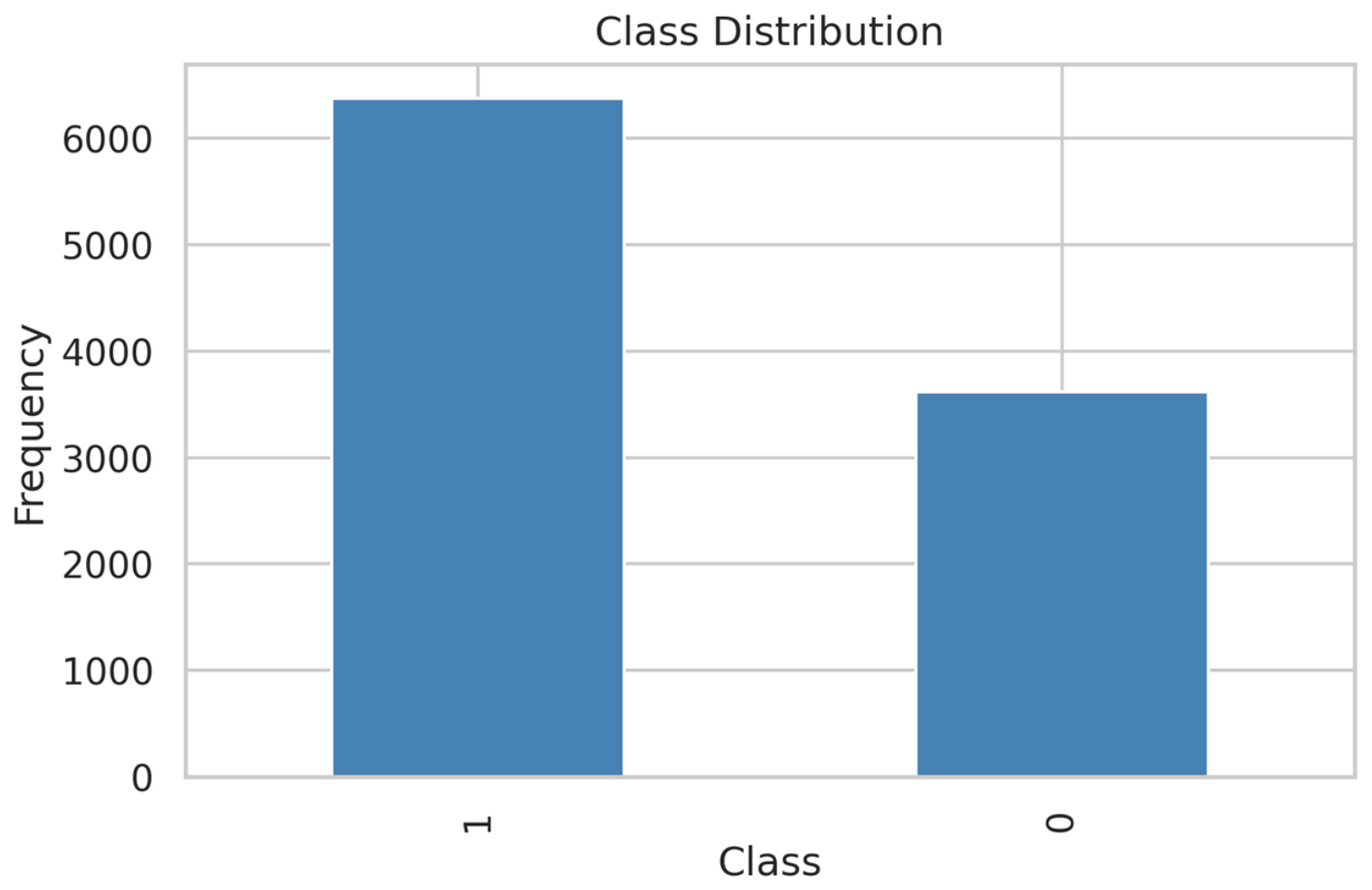The target value consists of the variable “stab,” which denotes the maximum real component of the characteristic equation root (a positive stab signifies linear instability). The dependent variable of this study is “stabf,” which classifies the system’s stability as either stable or unstable. 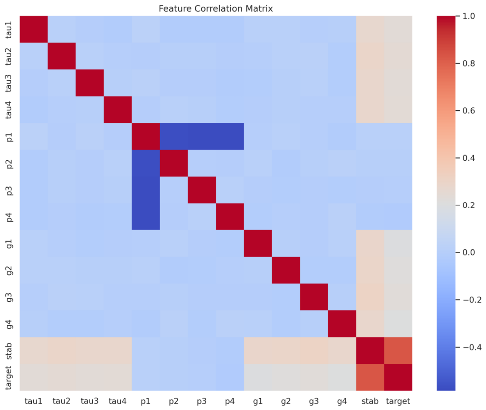The distribution of target variables exhibits a substantial imbalance, with 6380 instances in Class 1 and 3620 instances in Class 0, as depicted in Figure 1. Although the imbalance is not severe, it may nonetheless introduce bias favoring the majority class during model training if appropriate precautions are not included. A robust correlation is evident between ‘stab’ and ‘stabf’ (Refer to Figure 2). Consequently, the predictive attribute ‘stab’ was excluded from consideration as a predictive feature and dismissed.

Note that the UCI Smart Grid Stability dataset does not contain measurement noise, missing sensor data, communication failures, or concept drift, which may happen in a real smart grid. Thus, the focus of the present study is on the evaluation of the proposed framework in controlled environments, not in real deployment.

Algorithm 1: Sustainable hybrid deep learning framework with statistical validation

Input: Dataset ( D = {X, y} ), number of folds (K ), random seed ( S ) Output: Performance metrics, sustainability metrics, ROC curves, confusion matrices, statistical significance, ranked models Phase 1: Data Preprocessing       1: Set random seed ( s ) for reproducibility       2: Load dataset ( D )       3: Encode target variable ( y ) using label encoding       4: Remove irrelevant features from ( X )       5: Normalize ( X ) using Min-Max scaling       6: Reshape ( X ) into 3D tensor for deep learning models Phase 2: Model Definition and Initialization 7: Define Fusion Model Components:  ● eXtreme Gradient Boosting (XGBoost) as a strong gradient boosting classifier  ● Random Forest (RF) as a bagging-based robust learner  ● CNN as a deep feature extractor producing probabilistic outputs Phase 3: Fusion Model Training with Cross-Validation 8: Apply Stratified K-Fold Cross-Validation on dataset D 9: For each fold i = 1 to K do 10: Split dataset into training and testing sets 11: Standardize input features using Min-Max Scaler (fit only on training set) (A) Base Learner Training (Fusion Inputs) 12: Train base models on training data  ● XGBoost → learns gradient boosting decision boundaries  ● Random Forest → learns bagged tree ensembles  ● CNN → learns non-linear feature representation from reshaped input 13: Predict probabilities on test set for each model (B) Fusion Strategy (Core Contribution) 14: Compute fused probability using adaptive soft voting 15: Generate final prediction Phase 4: Aggregation, Statistical Validation and Final Evaluation 16: Compute overall performance metrics, sustainability scores and rank models based on performance and sustainability 17: Compare with basic and DL models using T-test.

2.2. Data Preprocessing

To guarantee reproducibility, numerical stability, and compatibility with DL architectures, a structured preprocessing pipeline is used in this paper. The preprocessing stage is intended to bring raw data to a normalized and model-ready format without losing any information about classes and by reducing biasing effects of scaling or encoding functions. First, a fixed random seed ($s = 42$) is used to make sure that all computational libraries (NumPy 2.0.2, TensorFlow 2.0, operating system environment, and others) use the same random seed. This ensures determinism in splitting data, weight initialization, and training processes. The dataset is organized into input features (X) and target labels (y). The target variable is converted to numeric values using a label encoder technique that transforms the categorical stability labels into binary numeric values [16]. After that, the input features are all normalized using a min-max scaling technique that standardizes each input feature to a value in the ([0, 1]) range, which guarantees numerical stability and speeds up the convergence of the gradient-based learning models [17]:

$$X^{\prime } ={\displaystyle \frac{X - X_{\mathrm{m}\mathrm{i}\mathrm{n}}}{X_{\mathrm{m}\mathrm{a}\mathrm{x}} - X_{\mathrm{m}\mathrm{i}\mathrm{n}}}}$$

(1)

where $X$ is the original value, $X_{\mathrm{m}\mathrm{i}\mathrm{n}}$ the minimum value in the dataset, $X_{\mathrm{m}\mathrm{a}\mathrm{x}}$ the maximum value in the dataset, and $X^{\prime }$ the scaled value in the range [0, 1].

In order to allow sequential processing in recurrent neural networks (RNNs), the normalized feature matrix is reshaped into a 3D-tensor representation $X_{Reshaped}\in {\mathbb{R}}^{N\times F\times 1}$, where

• N is the number of samples;
• F is the number of features;
• 1 is the single-channel input used by the CNN architecture.

This transformation gives the opportunity to each feature vector to be viewed as a sequential input that can be utilized in the temporal feature extraction.

The dataset consists of independent static attributes, but it was restructured into a dataset with three dimensions as part of the same preprocessing pipeline for all the deep learning models that were used in the comparison, namely CNN, LSTM, and GRU. The order of features in the imposed does not indicate the temporal dependencies or physical sequences. As a result, recurrent models can create artificial dependencies that can have a detrimental impact on performance. Likewise, the CNN should be viewed as a local feature interaction extractor and not a temporal model. In the future, permutation-invariant and tabular-specific deep learning architectures will be explored that do not require feature ordering.

2.3. Model Definition and Initialization

In this paper, a probabilistic fusion framework that incorporates classical ML and DL models under a unified decision-making architecture is proposed. The aim of this model is to improve predictive performance while maintaining computational efficiency and interpretability. Let the dataset be denoted by

$$D={\left\{x_i, y_i\right\}}_{i=1}^N, x_i\in {\mathbb{R}}^d, y_i\in \{0,1\}$$

(2)

where N represents the number of samples, and d is the feature dimensionality.

• Classical Machine Learning Models

In this model, two classical ML methods are used:

• eXtreme Gradient Boosting (XGBoost), which is considered an additive ensemble of K regression trees; the prediction for sample $i$, ${\widehat{y}}_i$, is given by [18]

  $${\widehat{y}}_i={\sum }_{k=1}^K{f}_k\left(x_i\right),f_k\in \mathrm{Ϝ}$$

  (3)

  where $\mathrm{Ϝ}$ is the space of decision trees. The regularized objective function is defined as

  $$L_{\theta }={\sum }_{i=1}^{N}l(y_i,{\widehat{y}}_i)+{\sum }_{k=1}^K{\mathsf{\Omega }}_{f_k}$$

  (4)

  where (l(.)) is a differentiable loss function (log-loss for binary classification), and the regularization term is

  $${\mathsf{\Omega }}_{\mathrm{f}}=\mathsf{{\rm Y}}T+{\displaystyle \frac{1}{2}}\lambda {\left|\mathrm{w}\right|}^2$$

  (5)

  where T is the number of leaves, w is the leaf weight vector, $\mathsf{{\rm Y}}$ is the complexity penalty, and $\lambda$ is the L2 regularization coefficient. This representation guarantees the control of the complexity of the XGBoost model and reduces the possibility of overfitting.
• Random Forest (RF), which consists of building an ensemble of M decision trees trained on bootstrap samples. The final prediction $\widehat{y}\left(x\right)$ is given as an average of all trees [19]:

  $$\widehat{y}\left(x\right)={\displaystyle \frac{1}{M}}{\sum }_{m=1}^M{T}_m\left(x\right)$$

  (6)

  where each tree ($T_m$) is trained independently using random feature selection, improving variance reduction and robustness.

B.

Deep Learning Model (CNN Feature Extractor)

The CNN works based on reshaped input $x\in {\mathbb{R}}^{d\times 1}$. The proposed CNN is composed of three parts:

• Convolutional Feature Extraction, formulated as [20,21]

  $$h^l=\sigma (W^l\ast x+b^l)$$

  (7)

  where $W^l$ is the convolution kernel, (*) is the convolution operator, $b$ is the bias, and $\sigma (.)$ is the nonlinear activation function.
• Feature Representation, which is obtained after the convolution and flattening steps, and it is formulated as

  $$z_{CNN}={\mathrm{\varnothing }}_{CNN}\left(x\right)$$

  (8)
• Classification Layer, in which the probability of the output is computed based on

$$P_{CNN}\left(y=1/x\right)=\sigma (W{z}_{CNN}+b)$$

(9)

Using this structure, the CNN model acts as a nonlinear feature extractor and a probabilistic classifier.

2.4. Fusion Model Training with Cross-Validation

The proposed fusion framework integrates different heterogeneous learners by aggregating probabilistic outputs in a late-fusion ensemble strategy that ensures robustness and interpretability [22]. First, each base model provides a posterior probability, such as $P_{XGBoost}(y=1|x),P_{RF}(y=1\left|x\right),\mathrm{a}\mathrm{n}\mathrm{d} P_{CNN}(y=1|x)$. These probabilities are assumed to be conditionally independent estimators of the true posterior distribution. The final prediction is computed based on a weighted convex combination [23]:

$$P_{Fusion}\left(y=1|x\right)={\sum }_{m=1}^M{w}_m{P}_m\left(\mathrm{y}=1|x\right), w_m\ge 0, {\sum }_{m=1}^M{w}_m=1$$

(10)

where $w_m$ is the weight assigned to the $m$-th model and represents its relative contribution to the final fused prediction, with $w_m\le 0$ and ${\sum }_{m=1}^M{w}_m=1$.

In this paper, $P_{Fusion}$ is computed based on

$$P_{Fusion}=w_1{P}_{XGBoost}+w_2{P}_{RF}+w_3{P}_{CNN}$$

(11)

The fusion weights are computed by maximizing validation AUC values.

The binary prediction is computed finally as

$$\widehat{y}=I\left(P_{Fusion}\le \tau \right),\tau =0.5$$

(12)

where $I(.)$ is the indicator function. The proposed fusion architecture is theoretically justified by the diversity principle of ensemble learning, where the combination of diverse learners improves overall generalization capability by leveraging different inductive biases. In particular, XGBoost provides strong decision boundaries through residual error minimization via Gradient Boosting, whereas RF increases model robustness by reducing variance through bootstrap aggregation and random feature selection. The CNN component offers deep feature extraction via nonlinear abstraction via hierarchical feature learning. As a result, the fusion mechanism brings these complementary advantages together into a collective predictive model, which can be formally described as the simultaneous reduction of bias (deep representation), variance (ensemble averaging), and improved feature expressiveness (nonlinear feature transformation). The proposed fusion model guarantees bias reduction, variance reduction, and representation learning.

The fusion weights were optimized by performing a validation-based grid search over the range of plausible convex combinations of weights ($w_i\ge 0, \sum w_i=1$). The validation set was used to test the candidate weight combinations for each fold of the stratified 5-fold cross-validation, and the one that achieved the highest mean AUC was kept. The final weights obtained were 0.4, 0.3, and 0.3 for XGBoost, Random Forest, and CNN, respectively. The optimized weights were then set in the test to provide an unbiased assessment. While the strategies for this benchmark dataset were effective, adaptive weight-learning strategies will be investigated in future work, which would improve robustness under dynamic real-world smart grid conditions.

2.5. Aggregation, Statistical Validation and Final Evaluation

In this paper, all performance metrics are calculated across all K folds. The mean and standard deviation are then computed. To produce robust evaluation and comparison, the Friedman and Nemenyi tests are used to compare the performance of the models pairwise. Thus, the performance differences between the models can be checked to see if they are statistically significant.

In each model m, the confusion matrix CMs of every fold ($i \in \{1,2,\dots ,K\}$) are averaged up to obtain a global CM [24]:

$$C{M}_{average}^m={\displaystyle \frac{1}{K}}{\sum }_{i=1}^{K}C{M}_i^m$$

(13)

where the CM is illustrated in

Table 2. Confusion matrix for binary classification summarizing true and false predictions after comparing the model predictions to the true labels.

	Predicted Positive	Predicted Negative
Actual Positive	TP (True Positive)	FN (False Negative)
Actual Negative	FP (False Positive)	TN (True Negative)

.

Table 3. Performance and sustainability metrics with their mathematical formulas and corresponding descriptions.

Metric Name	Mathematical Formula	Description
Accuracy (ACC)	$ACC={\displaystyle \frac{TP+TN}{TP+TN+FP+FN}}$	Computes the overall ratio of correctly classified samples between all samples.
Precision	$Precision={\displaystyle \frac{TP}{TP+FP}}$	Represents the part of correctly predicted positive instance between all predicted positives.
True Positive Rate (TPR)	$TPR={\displaystyle \frac{TP}{TP+FN}}$	Also called recall; evaluates the ability of the model to correctly identify positive instances.
F1-Score	$F1=2\times {\displaystyle \frac{precision\ast recall}{precision+recall}}$	Harmonic mean of Precision and Recall, offering a balance between both measures.
False Positive Rate (FPR)	$FPR={\displaystyle \frac{FP}{FP+TN}}$	Measures the ratio of negative instances incorrectly classified as positive by the model.
AUC (Area Under Curve)	$AUC={\int }_0^{1}TPR\left(FPR\right)d\left(FPR\right)$	Represents the overall ability of the model to discriminate between classes across all thresholds. AUC = 1 for perfect classifier.
$C{O}_2$ Emissions	$C{O}_2={\displaystyle \frac{P·t}{1000·3600}}\gamma$	Estimates the carbon footprint based on energy consumption during model training.
Memory Usage (MB)	$M=M_{after}-M_{before}$	Measures the memory consumed during model training and execution.
Runtime (s)	$T=t_{end}-t\_\left(start\right)$	Represents the computational time required to train the model.
Normalized AUC	$AU{C}_{norm}={\displaystyle \frac{AUC-{AUC}_{min}}{{AUC}_{max}-{AUC}_{min}}}$	Scales AUC values between 0 and 1 for fair comparison across models.
Normalized ${CO}_{2 }$	${CO}_{2 norm}={\displaystyle \frac{C{O}_{2max}-C{O}_2}{C{O}_{2max}-C{O}_{2min}}}$	Inverse normalization where lower emissions yield higher scores.
Normalized Memory	$M_{norm}={\displaystyle \frac{M_{max}-M}{M_{min}-M_{\mathrm{m}\mathrm{a}\mathrm{x}}}}$	Assigns higher scores to models with lower memory consumption.
Normalized Runtime	$T_{norm}={\displaystyle \frac{T_{max}-T}{T_{min}-T_{\mathrm{m}\mathrm{a}\mathrm{x}}}}$	Rewards models with faster execution time.
Sustainability Score	$S=0.4. AU{C}_{norm}+0.2· CO{2}_{norm}+0.2· M_{norm}+0.2· T_{norm}$	Composite metric balancing predictive performance and sustainability factors. The weights of the equation reflect a trade-off between maximizing the predictive performance represented by AUC and minimizing the environmental impact (CO2 emissions), model complexity, and execution time.

summarizes the main performance metrics used to evaluate the different models [25,26,27].

For computing the carbon emissions, Python’s time tool is used to calculate the running time, and a library called “psutil” is employed to track memory usage. All experiments are done on the same computer for fair comparison between models. Since direct power measurements were not available, carbon emissions were estimated based on the model execution time using a constant CPU emission factor [28]. Therefore, the provided CO₂ values refer to an estimate of relative carbon emissions in the same experimental situations instead of absolute carbon footprints corresponding to a particular electricity grid or energy mix.

The weights of the sustainability score (0.4 for normalized AUC and 0.2 for each of the normalized CO₂ emissions, memory usage, and runtime) were empirically determined to capture the main goal of achieving high predictive performance while raising the importance of the variables representing computational efficiency and environmental impact. The weighting scheme is not the result of an optimization algorithm but is based on the understanding that it represents a manageable compromise between predictive performance and Green AI goals. This heuristic weighting is suitable for the current benchmark study, but further research is needed to enable adaptive and data-driven weight estimation in various deployment scenarios through multi-objective optimization and multi-criteria decision-making techniques.

To conduct a robust comparison among the different models, the Friedman test is employed to assess whether statistically significant differences exist in model performance across cross-validation folds based on AUC scores. Unlike pairwise parametric tests, the Friedman test does not assume normal data distribution and is well-suited for comparing the performance of multiple classifiers across repeated experiments or cross-validation folds. For each fold $i$, models are ranked based on their AUC performance, where rank 1 is given to the best-performing model. The Friedman test statistic is computed as follows [29]:

$${\mathsf{{\rm X}}}_F^2={\displaystyle \frac{12K}{M(M+1)}}\left[{\sum }_{j=1}^M{R}_j^2-{\displaystyle \frac{M{\left(M+1\right)}^2}{4}}\right]$$

(14)

where K is the number of cross-validation folds, M represents the number of compared models, and $R_j$ illustrates the average rank of model j across all folds.

The null hypothesis $H_0$ assumes that all models have equivalent performance (average ranks are equal). The validation of $H_0$ means there is no significant difference between the $M$ models across the $K$ folds. The alternative hypothesis $H_1$ assumes at least one model performs significantly differently. Both hypotheses are defined as follows:

$$\left\{\begin{array}{cc}{H}_0:& R_1= R_2=\cdots =R_M\\ H_1:& \exists i\ne j {such that R}_i\ne R_j\end{array}\right.$$

(15)

The difference between two models is considered statistically significant if p < 0.05.

If the Friedman test rejects the null hypothesis ((p < 0.05)), a Nemenyi post hoc test is conducted to identify which pairs of models differ significantly in terms of their average ranks. The critical difference, CD, between two models is computed using [30]

$$CD=q_{\alpha }\sqrt{{\displaystyle \frac{M(M+1)}{6K}}}$$

(16)

where $q_{\alpha }$ is the critical value based on the Studentized range statistic at significance level $\alpha$.

Two models are considered significantly different if the absolute difference between their average ranks exceeds the critical difference:

$$\left|R_i-R_j|>CD\right.$$

(17)

For each model (m), the overall performance and sustainability metrics are computed using

$$AU{C}^m={\displaystyle \frac{1}{K}}{\sum }_{i=1}^{K}AU{C}_i^m$$

(18)

$$AC{C}^m={\displaystyle \frac{1}{K}}{\sum }_{i=1}^{K}AC{C}_i^m$$

(19)

$${F1}^m={\displaystyle \frac{1}{K}}{\sum }_{i=1}^K{F1}_i^m$$

(20)

$${CO}_2^m={\displaystyle \frac{1}{K}}{\sum }_{i=1}^K{C{O}_2}_i^m$$

(21)

$$M^m={\displaystyle \frac{1}{K}}{\sum }_{i=1}^K{M}_i^m$$

(22)

$$T^m={\displaystyle \frac{1}{K}}{\sum }_{i=1}^K{T}_i^m$$

(23)

Unlike traditional evaluation techniques that focus solely on predictive performance, this benchmark study combines statistical validation with a Green AI-oriented assessment method that jointly evaluates AUC, runtime, memory usage, and estimated computational CO₂ emissions. This evaluation allows the selection of models that offer an effective balance between predictive accuracy and computational efficiency.

3. Results

This section shows and analyzes the outcomes of applying the methodology presented in Section 2 on the UCI dataset (described in Section 2.1). The results from the suggested prediction model are illustrated, discussed, and compared with fundamental ML and DL models. The experiment is performed on a workstation equipped with an Intel Core i7 processor (3.6 GHz), 32 GB of RAM, and an NVIDIA RTX 3060 graphics card. The fusion model CNN–RF–XGBoost proposed in this paper was implemented in Python 3.12.12. Deep learning models were created with TensorFlow 2.19.0/Keras, and classical machine learning with the scikit-learn and XGBoost libraries. The experiments were repeated using a fixed random seed (seed = 42) to improve repeatability. All ML models in this section are assessed using the identical data partition and common cross-validation folds to ensure a fair and consistent comparison.

LSTM and GRU models have been added only as a reference baseline to make a thorough comparison with the recurrent neural models. They are not part of the proposed fusion framework, which includes only CNN, XGBoost, and Random Forest. A unified preprocessing pipeline was used for all deep learning models to provide a fair comparison between models and to show that recurrent sequence models are not well suited for this tabular smart grid dataset.

The proposed CNN architecture consists of an input layer, as well as a 1D convolution layer made up of 16 filters with a kernel size of two, along with the ReLU activation function. The feature maps that were produced are then processed with the fully connected layer containing 16 neurons using the ReLU activation function. The output layer consists of a single neuron with the sigmoid activation function, allowing for binary classification of smart grid stability. The model was trained using the Adam optimizer, with a learning rate of 0.001, binary cross-entropy loss, a batch size of 32, and 50 training epochs. The training of the model followed the same data preprocessing and 5-fold stratified cross-validation as used for the models evaluated. The total number of parameters makes it a lightweight CNN architecture. The overall design of the proposed architecture was simplified to ease the computational complexity without losing predictive capabilities and thereby achieving the Green AI goals set by the study.

In order to conduct a reliable and systematic comparison among the assessed models of machine learning, hyperparameter tuning was carried out using GridSearchCV on the training data according to the stratified 5-fold cross-validation method. The combinations of hyperparameters produced candidates that were evaluated by means of cross-validation, having selected the combination that showed the highest average validation performance for the final model. Finally, the chosen hyperparameters were used in all experiments described in the work. When developing deep learning systems (CNN, LSTM, and GRU), the approach employed the same training configuration, where three and 50 epochs of training and the Adam optimizer, along with all the preprocessing, were identical to provide homogeneity to the resulting models.

3.1. Confusion Matrix and Performance Metrics

The parameters used for each model are illustrated in

Table 4. Hyperparameter settings for the different ML and DL models.

Model	Hyperparameter
Common Settings	5-Fold Cross-Validation, Random Seed = 42, Classification Threshold = 0.5, Feature Scaling = StandardScaler
XGBoost	Number of Trees = [120, 500], Maximum Depth = 4, Evaluation Metric = Logloss, Learning Rate = 0.3
Random Forest	Number of Trees (n_estimators) = [100, 500], Split Criterion = Gini, Maximum Depth = Default
CNN	Conv1D Filters = 16, Kernel Size = 2, Dense Units = 8, Activation = ReLU, Output Activation = Sigmoid, Optimizer = Adam, Epochs = [3, 50]
LSTM	LSTM Units = 16, Dense Units = 8, Activation = ReLU, Output Activation = Sigmoid, Optimizer = Adam, Epochs = [3, 50]
GRU	GRU Units = 16, Dense Units = 8, Activation = ReLU, Output Activation = Sigmoid, Optimizer = Adam, Epochs = [3, 50]
Fusion Model	Weighted Averaging (XGB = 0.4, RF = 0.3, CNN = 0.3), Decision Threshold = 0.5

. The average values of the confusion matrix from the five folds of the stratified cross-validation are shown in Table 4. For each model, the numbers of TP, TN, FP, and FN were calculated independently on each fold and then averaged over the five folds (

Table 5. Average confusion matrix values across the 5-fold stratified cross-validation for all evaluated models under two different configurations (XGB, RF, CNN, LSTM, GRU, and FUSION).

Configuration A: XGB (Number of Trees = 120), RF (Number of Trees = 100) Epochs = 3 (CNN, LSTM and GRU)					Configuration B: XGB (Number of Trees = 500), RF (Number of Trees = 500) Epochs = 50 (CNN, LSTM and GRU)
Model	TN	FP	FN	TP	TP	FP	FN	TP
XGB	225.8	25.4	14.4	234.4	292.8	7	4.4	295.8
RF	225.8	25.4	13.4	235.4	291.8	8	5	295.2
CNN	222.6	28.6	15.4	233.4	289.8	10	9.2	291.0
LSTM	171.6	79.6	80.8	168.0	281.4	18.4	10.4	289.8
GRU	171.8	79.4	90.2	158.6	289.0	10.8	7.4	292.8
FUSION	243.4	7.4	4.2	244.9	294.2	5.6	3.2	296.8

). As such, the reported values are decimal numbers, not integer counts, of the means. For the first configuration (XGB (Number of Trees = 120), RF (Number of trees = 100), Epochs = 3 (CNN, LSTM and GRU)), the proposed fusion model shows the most desirable balance between the true positive and negative cases, with a high number of true positives (TP = 244.9) and true negatives (TN = 243.4) and low false negatives (FN = 4.2) and false positives (FP = 7.4). This suggests its strong ability to correctly classify both positive and negative instances with low classification errors. Other traditional ensemble approaches (XGBoost and RF) also show promising and balanced classification capability, with high TP and TN values, although they still incur slightly greater errors than the fusion model. Conversely, CNN demonstrates moderate classification performance with higher FPs, while the sequential DL models (LSTM and GRU) show much lower performance with higher FPs and FNs, suggesting poor capabilities in identifying discriminative features. Overall, these findings demonstrate that while stand-alone DL models may suffer from stability and misclassification issues, ensemble-based approaches, particularly the proposed fusion model, offer a better, more balanced, and reliable decision-making system for classification.

There was significant improvement in all the evaluated models in configuration B (XGB (Number of Trees = 500), RF (Number of trees = 500) and Epochs = 50 (CNN, LSTM and GRU)) that resulted from adding more trees to the ensemble classifiers and from increasing the number of epochs being used to train the deep learning models from three to 50 epochs. In addition, the extra training solved some false positives and false negatives for all the models, more specifically for LSTM and GRU models, showing that the lack of training caused their performance to drop significantly before the additional training. XGBoost was consistently the most powerful single classification model, with Random Forest providing similar performance. However, all the baselines were improved, and the proposed fusion model always had superior classification accuracy, with 294.2 TN, 296.8 TP, 5.6 FP, and 3.2 FN, which represented the minimum overall misclassification rates. These results highlight the ability of the fusion framework to align the complementary power of the machine learning and deep learning models and to keep predictive ability at a high level, even in a more challenging and fair training setting (see Table 5).

Table 6. Performance comparison of the proposed model and the basic ML and DL models based on key evaluation metrics.

Configuration A: XGB (Number of Trees = 120), RF (Number of Trees = 100) Epochs = 3 (CNN, LSTM and GRU)						Configuration B: XGB (Number of Trees = 500), RF (Number of Trees = 500) Epochs = 50 (CNN, LSTM and GRU)
Model	Accuracy	F1-score	Precision	Recall	AUC	Accuracy	F1-score	Precision	Recall	AUC
XGB	0.9204	0.9217	0.9023	0.9421	0.9692	0.9810	0.9814	0.9769	0.9854	0.9956
RF	0.9224	0.9239	0.9027	0.9461	0.9683	0.9783	0.9788	0.9736	0.9840	0.9949
CNN	0.9120	0.9139	0.8911	0.9381	0.9609	0.9677	0.9684	0.9668	0.9700	0.9888
LSTM	0.6792	0.6753	0.6793	0.6753	0.7435	0.9510	0.9518	0.9402	0.9634	0.9816
GRU	0.6608	0.6505	0.6684	0.6375	0.7320	0.9682	0.9689	0.9644	0.9734	0.9897
CNN + RF	0.9219	0.9217	0.8991	0.9405	0.9687	0.9654	0.9782	0.9752	0.9812	0.9899
CNN + XGB	0.9180	0.9199	0.8989	0.9401	0.9653	0.9710	0.9755	0.9711	0.9801	0.9905
RF + XGB	0.9212	0.9228	0.9027	0.9444	0.9688	0.9800	0.9801	0.9755	0.9849	0.9950
FUSION	0.9768	0.9766	0.9859	0.9811	0.991	0.9849	0.9853	0.9815	0.9893	0.9978

illustrates the performance metrics of the proposed fusion models compared to the basic ML and DL models under the two configurations (A and B). For the first configuration, the findings clearly show that the proposed fusion model outperforms other models, with an accuracy of 0.9768, a precision of 0.9766, a recall of 0.9859, and an F1-score of 0.9811, showing high classification accuracy, high sensitivity, and a low misclassification rate. This demonstrates the value of creating an ensemble of diverse learners to effectively control both FP and FN rates. The traditional ensemble methods, XGBoost and RF, also perform well and consistently. RF performs slightly better than XGBoost in terms of accuracy (0.9224 vs. 0.9204) and F1-score (0.9240 vs. 0.9216), but XGBoost achieves competitive recall (0.9421), thus being able to capture positive instances. The CNN model performs reasonably well, with similar precision and recall, delivering an accuracy of 0.9120 and an F1-score of 0.9140, but is still outmatched by ensemble methods. However, the recurrent DL models (LSTM and GRU) demonstrate limited predictive performance, with accuracies of 0.6792 and 0.6608, respectively. This is reflected in their lower levels of precision, recall, and F1-scores, suggesting that they are not as effective in handling tabular data without feature engineering or ensemble learning.

Table 6 also shows that the performance of all classifiers improves with a higher number of trees for the ensemble models and with longer deep learning training (50 epochs)—this is configuration B. XGBoost was the best single model, with an accuracy of 98.10% and an AUC of 99.56%, with Random Forest also performing well. The CNN, LSTM, and GRU models also performed significantly better, especially LSTM and GRU, which are recurrent models, highlighting the need for proper training of deep learning models. Nevertheless, the proposed fusion model consistently achieved the best overall results, with an accuracy of 98.49%, F1-score of 98.53%, precision of 98.15%, recall of 98.93%, and AUC of 99.78%. The results indicate that the ensemble learning and deep feature extraction models are able to complement each other to achieve better prediction performance and robustness than each of them alone.

Table 6 demonstrates the effectiveness of the proposed fusion framework compared with standalone models (RF, XGBoost, and CNN) and simpler hybrid approaches (RF + CNN, RF + XGBoost, and CNN + XGBoost). For Configuration A, all models provide almost similar performance (approximately 92% accuracy), indicating that limited feature learning restricted accurate prediction. However, the fusion model outperforms all the standalone and hybrid models by reaching an accuracy of 97%. In Configuration B, increasing the CNN training to 50 epochs and expanding the ensemble models to 500 trees significantly improved all methods. The proposed fusion framework also achieved the best performance by reaching an accuracy of 98.53%. These results demonstrate that integrating CNN-extracted deep features with both RF and XGBoost effectively enhances model capability and results in a more accurate, robust, and reliable predictive model.

The underperformance of LSTM and GRU models is mainly due to their mismatch with the characteristics of the dataset, which is inherently tabular and non-sequential rather than time-series. However, these recurrent architectures are trained to capture temporal dependencies, which is not applicable in this context. Thus, they are inefficient in learning features. Furthermore, these models are more architecturally complex, which adds unnecessary parameters to the training network and creates instability during training without providing any advantages in discrimination. Tree-based ensemble techniques like XGBoost and Random Forest, however, work better with tabular data, as they tend to be more robust and capture nonlinear feature interactions more effectively, hence the performance difference with LSTM and GRU.

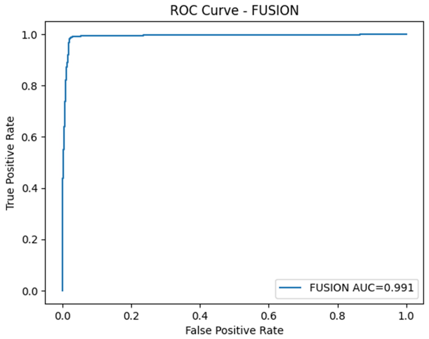
Figure 3 represents the ROC curve of the fusion model tested on the 5-fold cross-validation under Configuration A. The Area Under the Curve (AUC = 0.991) is large, demonstrating that the model has excellent discriminative ability between two classes. The curve is steeply increasing towards the top left, indicating that the model achieves a high true positive rate, even at extraordinarily low false positive rates, which is advantageous when accurate classification is required in highly important situations.

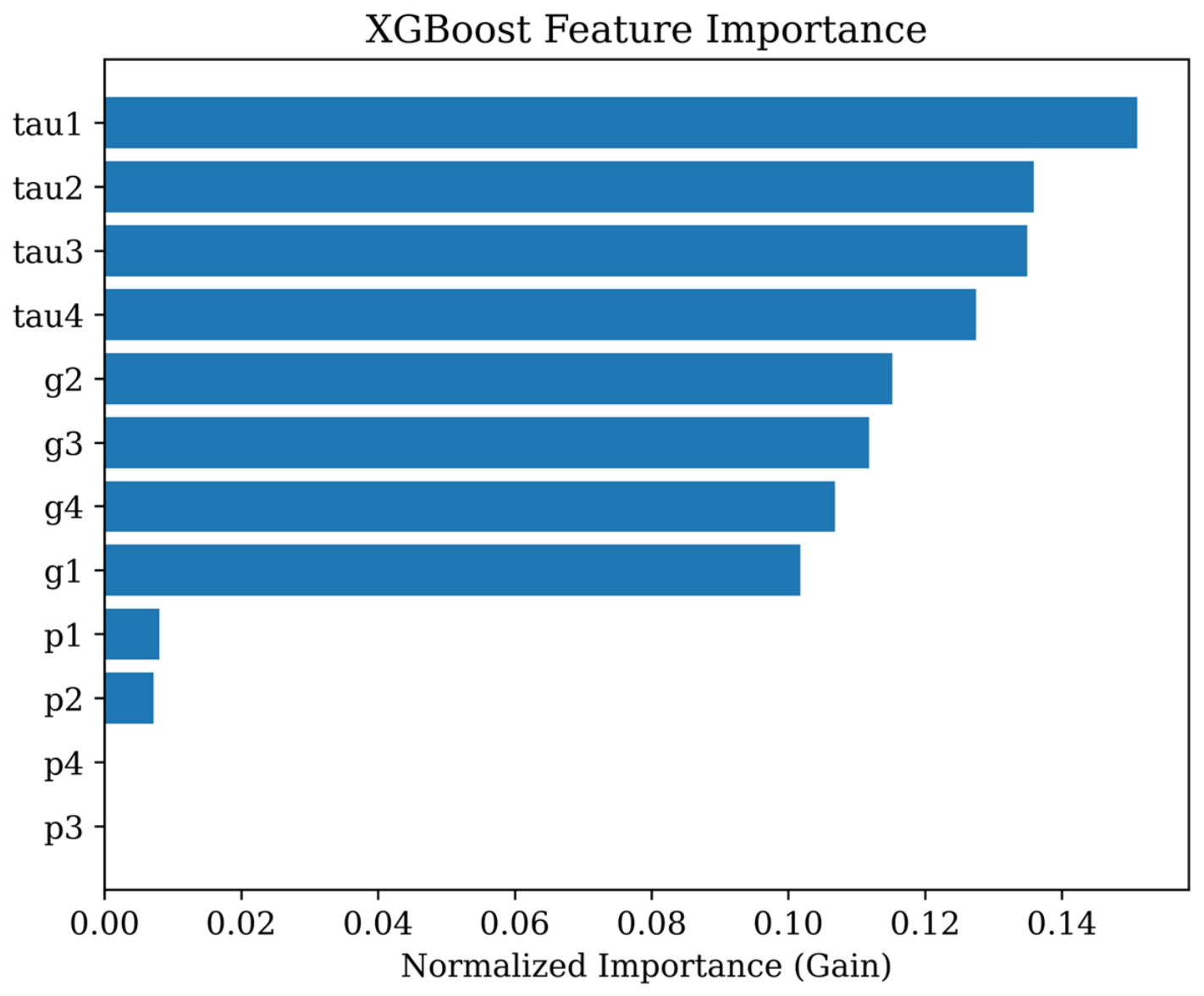
Figure 4 shows the feature values of the XGBoost in terms of normalized gain values that represent the relative contributions of each input variable to the predictive power of the model. The results show that the time-related characteristics (tau1–tau4) are the most significant, showing that the dynamics of time are dominant in determining the stability of the system. The other variables are less important since they are the generation-related variables (g2, g3, g4, and g1) and thus have a secondary but still significant influence on the decisions made by the model. The power-related attributes (p1, p2, p3, and p4), on the other hand, are of insignificant importance, implying less impact on the classification outcome in this case.

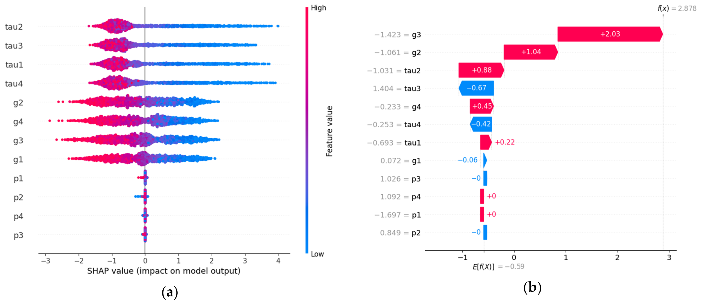
From the SHAP summary plot (see Figure 5a), it can be seen that the synchronization time constants (tau2, tau3, tau1, and tau4) and generator gain parameters (g2, g4, g3, and g1) are the most impactful variables influencing the XGBoost model predictions, whereas the active power parameters (p1–p4) show negligible impact, as the SHAP values are centered around zero. From the color distribution, it is possible to conclude that smaller values of the tau parameters contribute to the probability of system instability, while larger values tend to have a smaller contribution due to the nonlinear dependencies captured by the model. As can be seen from the SHAP waterfall plot (see Figure 5b), g3, g2, and tau2 are the main variables that drive the prediction towards the stable class and increase the model output score, while tau3 and tau4 somewhat oppose this tendency and decrease the prediction score. Other features have only small effects on the prediction outcome. The achieved explainability of the model proves that the proposed XGBoost classifier takes into account physical features of the electrical grid and thus increases the interpretability of the model.

3.2. Sustainability Evaluation

Table 7. Comparison of sustainability metrics between fusion and all models.

Configuration A	Model	Norm AUC	Norm CO2	Norm Memory	Norm Runtime	Sustainability Score
	XGBoost	0.969	0.827	0.200	0.750	0.783
	RF	0.968	0.000	0.000	0.880	0.563
	CNN	0.961	0.015	1.000	0.820	0.787
	LSTM	0.744	0.015	0.7132	0.3554	0.311
	GRU	0.732	0.015	0.520	0.000	0.400
	FUSION	0.991	1.000	0.030	0.998	0.802
Configuration B	XGBoost	0.998	0.620	0.150	0.420	0.637
	RF	0.997	0.580	0.120	0.390	0.617
	CNN	0.989	0.350	0.850	0.520	0.720
	LSTM	0.982	0.280	0.600	0.310	0.631
	GRU	0.987	0.280	0.515	0.289	0.611
	Fusion	0.997	0.7	0.585	0.595	0.775

offers a comparative sustainability assessment, indicating clear trade-offs between predictive performance and computational efficiency across the proposed and basic models. The proposed fusion model achieves the highest sustainability score (0.802). Compared with XGBoost (0.783), it provides an improvement of approximately 2.4% while also outperforming the remaining benchmark models and demonstrates a significant improvement of 37.4% over RF, 50.6% over LSTM, and 93.5% over GRU. This gain is primarily driven by its superior normalized AUC (0.991) combined with the best CO₂ efficiency (1.000) and near-optimal runtime (0.998), despite its relatively low memory efficiency (0.030). While CNN (0.751) shows competitive sustainability, its advantage is largely attributable to perfect memory efficiency (1.000), which mitigates its weak CO₂ performance (0.015). These values indicate a structural imbalance, as the model appears sustainable primarily due to one favorable metric rather than a genuinely efficient overall design. However, XGBoost (0.743) shows a well-balanced profile, with strong CO₂ efficiency (0.827) and high AUC (0.969), but its sustainability is limited by moderate memory efficiency (0.200), demonstrating its sensitivity to the overall score of resource utilization. The RF model (0.563) performs rather poorly and scores roughly 27.3% lower on sustainability than the fusion model. Even though it yields a similar AUC score (0.968), its much lower CO₂ and memory efficiency scores (0.000 for both) indicate that the ensemble approach requires more energy and computation and is less suitable for sustainable usage. Additionally, the individual DL models suffer significantly from inefficiencies. While the LSTM and GRU scores of 0.514 and 0.400, respectively, are 33.6% and 48.3% lower than the fusion score, this is mainly due to their higher running times and resource usages (0.355 normalized running time for LSTM and 0.000 for GRU). In spite of achieving adequate predictive performances (AUC of 0.744 and 0.732), their poor sustainability is largely attributed to these deficits, suggesting that a satisfactory AUC score alone does not outweigh the higher computational cost.

In general, these results point to the fact that individual DL models cannot efficiently perform both accurate prediction and sustainable usage simultaneously. The fusion model, on the other hand, shows that combining models can make them more accurate and efficient. Nonetheless, we must acknowledge that the fusion model still possesses low memory efficiency, meaning that there are more optimizations to be made to reduce resource utilization, such as implementing more efficient algorithms or reducing model complexity.

For ensemble models, there was a clear increase in predictive ability, with an increase in the number of trees and with deep learning training extended to 50 epochs in Configuration B. The sustainability scores of XGBoost (0.637) and RF (0.617) were reduced due to the increase in computational complexity, although they had the highest AUC. The two models trained for longer, CNN and LSTM, performed better with higher AUC values and better overall performance. The fusion model demonstrated the best predictive performance (AUC = 0.997) and sustainability (0.775), showing a favorable compromise between prediction and computation. In summary, the results demonstrate that optimized fusion schemes can yield better prediction accuracy than single models, without compromising on sustainability.

3.3. Statistical Significance Analysis Using Friedman and Nemenyi Tests

In this subsection, Configuration A will be used for all the models. The average values of AUC and the corresponding 95% confidence intervals are illustrated in

Table 8. Mean AUC with 95% confidence intervals across 5-fold cross-validation.

Model	AUC	95% Confidence Interval
XGBoost	0.9692	[0.9878, 0.9979]
Random Forest	0.9683	[0.9828, 0.9992]
CNN	0.9609	[0.9813, 0.9965]
LSTM	0.7435	[0.5228, 1.0279]
GRU	0.7320	[0.4728, 0.5148]
Fusion	0.991	[0.9864, 0.9983]

, as obtained through five-fold cross-validation. The fusion model showed a lot of potential, achieving an AUC of 0.991, much higher than the scores achieved by other machine learning techniques such as XGBoost (0.9692) and Random Forest (0.9683), as well as deep learning approaches, including CNN (0.9609), LSTM (0.7435), and GRU (0.7320). The variability of the models can be estimated from the confidence intervals, while the result of the fusion model indicates that combining classifiers makes the system more reliable and recognizable.

As illustrated in

Table 9. Fold-wise AUC results of all models. The Friedman test indicates statistically significant differences among models (χ² = 22.49, p = 0.00042 < 0.05). The Nemenyi post hoc test uses a critical difference (CD = 3.37) to determine pairwise significance.

Fold	XGB	RF	CNN	LSTM	GRU	FUSION
1	0.9658	0.9663	0.9601	0.7322	0.7045	0.9868
2	0.9627	0.9614	0.9521	0.7547	0.7543	0.9900
3	0.9694	0.9708	0.9591	0.7310	0.5332	0.9911
4	0.9750	0.9772	0.9677	0.7621	0.7396	0.9888
5	0.9729	0.9646	0.9627	0.7567	0.7507	0.9924

, the proposed fusion model achieves the higher AUC value across all folds (0.9868–0.9924) as compared to XGBoost and RF by approximately 1.5–2.5%. The CNN model’s performance is excellent and reaches a higher AUC than LSTM and GRU. The non-parametric test, the Friedman test, confirms overall significant differences (p < 0.05) among the models’ performances without assuming data normality. However, the Nemenyi analysis indicates that the fusion model is only statistically superior to LSTM and GRU (see

Table 10. Nemenyi post hoc pairwise comparison (CD = 3.37).

Comparison	ΔRank	Significant Difference
FUSION vs. XGB	0.60	No
FUSION vs. RF	0.60	No
FUSION vs. CNN	2.40	No
FUSION vs. LSTM	3.40	Yes
FUSION vs. GRU	4.40	Yes
XGB vs. RF	0.00	No
XGB vs. CNN	1.80	No
XGB vs. LSTM	2.80	No
XGB vs. GRU	3.80	Yes
RF vs. CNN	1.80	No
RF vs. LSTM	2.80	No
RF vs. GRU	3.80	Yes
CNN vs. LSTM	1.00	No
CNN vs. GRU	2.00	No
LSTM vs. GRU	1.00	No

), while the differences with XGBoost, Random Forest, and CNN are not statistically significant. The results are aligned with the sustainability analysis performed, where the fusion model achieves the top sustainability score, as it balances predicted performance and computational resources, as well as environmental aspects, more optimally, making it a suitable choice.

Table 11. Effect size (Cohen’s d) between the proposed fusion model and baseline models. Effect size interpretation follows Cohen’s guidelines: negligible (<0.20), small (0.20–0.49), medium (0.50–0.79), and large (≥0.80).

Comparison	Cohen’s d	Effect Size Interpretation
Fusion vs. XGBoost	−0.111	Negligible
Fusion vs. Random Forest	0.229	Small
Fusion vs. CNN	0.630	Medium
Fusion vs. LSTM	1.508	Large
Fusion vs. GRU	40.065	Extremely Large

, specified in the eleventh section, shows the effect size of performance difference based on Cohen’s d. The fusion model reported significant improvement when compared to representation models like CNN, LSTM and GRU. However, the effect size in comparison with XGBoost was found to be insignificant.

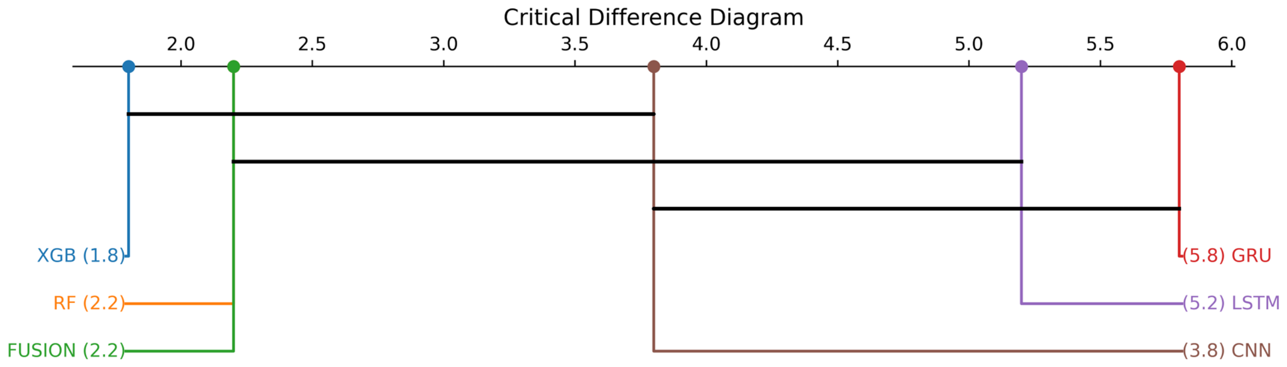
The critical difference (CD) plot obtained from the Friedman test and the Nemenyi post hoc comparison can be seen in Figure 6. Based on this figure, the suggested fusion model showed one of the highest average ranks and belonged to the same group as XGBoost and Random Forest, implying no performance differences among these models. In contrast, CNN, LSTM, and GRU were classified into groups with lower ranks, reflecting weaker prediction ability. These findings corroborate the results derived from the AUC analysis and prove the efficacy of the suggested fusion approach in terms of performance.

3.4. Complexity and Scalability Analysis

The complexity and scalability of the proposed CNN–RF–XGBoost fusion network are also taken into account, aside from predictive performance evaluation. The proposed architecture is a combination of three models having complementary computational features. The computational cost of the CNN component is primarily related to the number of convolutional filters, kernel size, input feature dimensions, and number of training samples. The adopted CNN architecture is lightweight, so it has a linear computational complexity during training and inference as the size of the data grows. The complexity of the Random Forest component is primarily determined by the number and depth of the trees ($O(M N log N)),$ with M being the number of trees and N being the number of samples. Likewise, the complexity of XGBoost is related to the number of boosting trees (K), depth of the boosting trees (d), and size of the training dataset (N) and is estimated as $O(K N log N).$ The overall computational cost of the proposed fusion strategy is roughly the sum of the computation cost of individual models because the predictions of the separately trained models are fused.

As for scalability, the proposed framework can perform efficiently with larger datasets, as the CNN, RF, and XGBoost components are able to process the samples independently and can also be parallelized. The experimental results on UCI Smart Grid Stability data (10,000 samples and 12 predictive features) show that the model obtains a good balance between its predictive capabilities and computational demands by using runtime, memory usage, estimated CO₂ emissions, and sustainability score. The proposed lightweight CNN feature extractor and efficient tree-based ensemble learners not only preserve high classification performance but also reduce computational overhead. But the large-scale deployment scenarios, such as high-frequency measurements, smart grid stream data, and heterogeneous sensor network generation, can present further computational difficulties. To increase scalability for real-time smart grid applications, future work will explore additional ways to optimize, such as model compression, online learning, and distributed implementations.

3.5. Discussion and Comparison

The comparative results in

Table 12. Comparison of the proposed FUSION approach with existing models.

Study	ML Models	Accuracy (%)
Aziz et al. in [31]	Ensemble Bagging Technique	90.16
Ibrar et al. in [32]	XGBoost	96.8
Wang et al. [33]	CatBoost	94.4
Chahal et al. [34]	ANN	97.27
Alsirhani et al. [9]	MLP	95.8
Khaleefah et al. [35]	LSTM	96.73
Proposed Fusion approach	Soft Voting: CNN, RF, XGBoost	98.49

indicate that ensemble-based approaches remain the most effective for power system stability prediction; however, the findings no longer support the dominance of a single model such as XGBoost. As shown in Table 9, the proposed fusion approach (CNN + RF + XGBoost) achieves the highest accuracy of 97.68%, outperforming both the standalone XGBoost model (96.8%) and earlier ensemble methods such as bagging (90.16%) reported in prior studies. This corresponds to an improvement of approximately +1.2% over XGBoost and +7.8% over traditional ensemble techniques, highlighting the benefit of combining heterogeneous learners. While XGBoost remains a strong and reliable baseline due to its high precision and robustness, the results demonstrate that its performance can be further enhanced through model fusion. The fusion strategy effectively integrates complementary strengths: CNN contributes feature extraction capability, RF improves variance reduction, and XGBoost provides strong boosting-based generalization. This synergy explains the consistent performance gains observed across folds. Additionally, the proposed voting fusion model outperforms traditional MLP, ANN, LSTM, and CatBoost-based approaches, indicating the superiority of hybrid ensemble learning in catching complementary feature representations compared to individual DL and gradient-boosting frameworks.

The results obtained with the proposed fusion framework are better than any of the others in terms of prediction accuracy and sustainability on the benchmark dataset; however, the results are not considered to have been obtained in a robust manner in the practical deployment conditions. The current evaluation is just one simulated dataset and hence does not measure resilience to sensor noise, missing data, communication noise, concept drift, and distribution shifts among various power systems. These conditions need to be validated experimentally to justify practical deployment.

3.6. Limitations

While the proposed Green-AI-aware fusion framework exhibits excellent predictive effectiveness, there are a number of limitations that should be recognized. The framework has only been tested on one benchmark dataset obtained by simulation of a four-node smart grid. Thus, the ability of the proposed method to be generalized to various smart grid topologies and operating environments in real-world conditions has not yet been proven. Moreover, the dataset is free from noisy sensor measurements, data loss, communication failures, and concept drift, which makes it impossible to evaluate the robustness of the proposed framework under realistic operating conditions.

Second, while the sustainability indicators include runtime and memory usage as well as estimated CO₂ emissions, these are indirect estimates and not measurements of the energy emitted by the hardware or a real carbon footprint in different computing scenarios. Third, the fusion approach is based on a pre-defined or empirically determined weight, compromising adaptability in dynamic and evolving grid conditions. Fourth, statistical significance testing (Friedman and Nemenyi) ensures the robustness of comparison, but a deeper uncertainty quantification analysis and confidence interval estimation for model predictions are not performed, and they are limited to classical non-parametric methods. Finally, the existing framework does not take into account real-time streaming data, concept drift, and deployment requirements in distributed smart grids and edge environments, which are important for the practical deployment of the industrial grid.

The weights were chosen to achieve high predictive accuracy along with computational efficiency and sustainability. Since there is importance in accurately predicting the stability of the smart grid, AUC was given more weight (0.4) in the evaluation process. All other criteria, including normalized carbon emissions, memory usage, and processing speed, were given equal weights (0.2) to balance and compare environmental impact and costs of the computation process. Despite the appropriateness of the weight scheme for practical evaluations, it does not claim to be the best possible scheme. Different applications can utilize different weights. That is why future research aims to carry out sensitivity analysis and apply some multi-criteria decision-making methods such as AHP or TOPSIS to search for proper weights for specific purposes and compare evaluation results with those achieved with the proposed weights above.

The feasibility of the proposed CNN–RF–XGBoost fusion framework is also explored in real-time smart grid applications. For stability prediction systems, inference latency is a key factor since a quick decision is crucial to avoid possible disturbances. After the training, inference can be done quickly thanks to the proposed architecture, which consists of a light CNN model for automatic feature extraction and efficient ensemble classifiers. Furthermore, the number of input features is relatively small, and the relatively compact model structure allows for lightweight deployment of the framework, such as on edge gateways or local monitoring devices. For highly constrained edge platforms, however, further optimization is needed to meet stringent latency and energy constraints, such as model pruning, quantization, knowledge distillation, and hardware acceleration. The proposed assessment considering Green AI is an initial indicator of computational suitability based on runtime, memory usage, and CO₂ emission analysis, although the evaluation is conducted on an open benchmark dataset. Future research will include testing the proposed framework in more practical settings. A series of experiments on robustness will be conducted using synthetic sensor noises, missing data scenarios, outlier contamination, and concept drift. Additionally, the framework is to be tested with larger real-world smart grid datasets and with a variety of datasets to check the generalization ability of the framework. These investigations will lead to more conclusive evidence of the appropriateness of the proposed solution for use in actual smart grid applications.

4. Conclusions

The rise in electricity demand resulting from technology breakthroughs and smart cities jeopardizes the stability of electrical systems. A reliable grid is essential for uninterrupted electricity supply, particularly as countries shift towards renewable energy sources such as solar, wind, and hydropower. The inconsistency in various sources hinders grid stability, leading researchers to suggest ways for evaluating SG stability. This paper proposes a Green AI-aware heterogeneous fusion framework that combines CNN, Random Forest, and XGBoost using validation-optimized soft-voting weights and evaluates the resulting model through a unified sustainability assessment that jointly considers predictive performance, execution time, memory usage, and carbon emissions. Soft voting is applied to combine the results of the Convolutional Neural Network with the XGBoost and Random Forest models. Also, the paper investigated the effectiveness of ML, DL, and hybrid approaches for power system stability prediction, with a special focus on performance, robustness, and sustainability. The proposed approach is tested and compared with a basic model using the UCI dataset. The experimental results demonstrate that the ensemble-based approaches, overall, perform better than stand-alone deep learning models. The proposed CNN–RF–XGBoost fusion approach is able to achieve competitive predictive performance with an accuracy of 98.0% and an AUC of 0.991 and to provide computational sustainability and a good balance between predictive power and sustainability.

The fusion model was found to achieve an accuracy of 98.0%, which is only slightly better than the accuracy of the individual baseline model and indicates the value of using a combination of the heterogeneous learners. Based on statistics, however, there is no statistical difference between the performance of the fusion model, XGBoost, and Random Forest, indicating that this improvement is considered to be a good enhancement and not a breakthrough in performance. Also, the fold-wise and statistical analyses further confirm that the proposed approach offers consistent and stable performance while significantly outperforming basic DL models such as LSTM and GRU. However, the absence of statistically significant differences between the fusion model and strong baselines like XGBoost and RF suggests that the improvement should be interpreted as a robust enhancement rather than a definitive breakthrough.

Furthermore, the sustainability assessment points out the trade-off between prediction accuracy and computation efficiency. Despite being highly efficient, XGBoost, the fusion model, demonstrates an improved balance of performance and resource utilization and thereby has a strong prospect of being applied to actual power systems in practice.

In conclusion, the results suggest that combining heterogeneous models with a fusion strategy provides a trustworthy and powerful approach for power system stability prediction. Future work can address larger-scale datasets, improved fusion techniques, and real-time deployment situations to validate and extend the presented framework to other domains. Several directions can be explored to further enhance the proposed framework. First, future studies should evaluate the model on larger and more diverse real-world power system datasets to improve generalizability and validate robustness under different operating conditions. Second, more advanced fusion strategies—such as adaptive weighting, stacking, or attention-based ensembles—could be investigated to further optimize the contribution of each base learner. In addition, integrating temporal and spatiotemporal features may improve the performance of deep learning components, particularly for dynamic stability scenarios. The use of automated hyperparameter optimization and neural architecture search could also enhance model performance while maintaining efficiency. From a sustainability perspective, future work should incorporate energy-aware training, model compression, and lightweight architectures to further reduce computational cost and environmental impact.

The proposed hybrid fusion framework is shown to have good predictive accuracy and computational efficiency on the benchmark UCI Smart Grid Stability dataset. But the present evaluation only involves controlled simulated data. Thus, although the framework has good potential for use in practical smart grid applications, further validation with noisy, incomplete, and real-world data is needed before it can be confidently backed up by deployment claims.