AI-Enabled Decision Support for Marine Pollution Assessment in High-Traffic Coastal Systems: Evidence from a 90-Day Multi-Site Pilot Study

Abstract

Coastal marinas and high-traffic nearshore sites accumulate pollution from vessel movements, tourism, and shifting weather, yet routine monitoring rarely operates at the temporal resolution needed to catch emerging risks before they become acute. This study developed an AI-enabled decision support system and tested it across three European coastal sites over a 90-day window in summer 2025: an urban marina (Site A), a tourism marina (Site B), and a mixed-use port channel (Site C). A composite Water Quality Risk Index (WQRI), combining five normalised environmental and vessel-traffic stressor dimensions, fed a two-layer AI framework in which a gradient boosting model estimated short-term traffic-related stress and a random forest model classified next-day risk. Vessel traffic was heaviest at Site B, but water quality risk followed a different pattern: Site C returned the highest mean WQRI and logged the most hours under red alert despite intermediate traffic volumes, indicating that sustained moderate traffic mattered more than peak volume. Vessel intensity and WQRI were positively correlated at all three sites, most strongly at Site B, and the next-day random forest risk classifier, trained across all three sites, achieved strong discriminative performance (AUC 0.93). When the system indicated elevated risk, managers responded by deploying inspections, issuing traffic advisories and increasing monitoring activity. The pilot shows that connecting vessel tracking, environmental sensing, and ML-based classification into a single decision loop can move coastal pollution management from reactive to anticipatory.

1. Introduction

Busy coastal zones, including marinas, port entrances, popular anchorages and tourist beaches, support multiple overlapping uses, and this concentration of activity creates substantial pollution pressures. Vessels leak hydrocarbons, discharge grey water, and disturb bottom sediments. Tourism infrastructure adds its own nutrient and wastewater loads. Stormwater carries road runoff across shorelines that were never designed to handle it. None of this is new. What has changed is the scale of global recreational boating and coastal tourism, both of which have expanded steadily over the past two decades.

In practice, this evidence gap has direct operational consequences. Coastal and marina managers are routinely asked to demonstrate progress against pollution-reduction targets, yet most have no systematic way of knowing which days, hours, or vessel movements were actually responsible for a given exceedance. Inspection and sampling budgets are allocated on fixed schedules or in response to public complaints rather than to evidence of elevated risk, so scarce staff time is frequently spent confirming that nothing unusual is happening while genuine short-duration pollution events pass undetected. The consequence is not merely a scientific blind spot: it is a recurring operational weakness in coastal management, in which the tools available to harbour masters and environmental officers lag well behind the pace at which pollution events actually unfold. Addressing this gap requires decision-support tools that operate at the same timescale as the risk itself, which is the practical problem this study addresses.

These pollution sources do not act independently. Vessel movements resuspend sediments that have accumulated antifouling compounds. Warmer surface waters from thermal stratification reduce the oxygen buffering capacity that would otherwise dilute an organic enrichment event. A summer squall can flush a marina basin just as peak visitor traffic is arriving. The resulting pollution signal is cumulative and highly location-specific. Consequently, the factors that matter at one site may be less important at another, and standard reference values may not adequately represent these interactions [1,2].

The central management problem is timing. Pollution events in busy coastal waters can develop and dissipate within hours. A water sample collected on Monday morning may show nothing unusual because the contamination peak passed on Sunday evening. Managers are structurally behind the problem because the data available to them describe what has already happened, and by the time an exceedance triggers a response, the causal conditions have often changed [3,4,5]. Routine monthly or weekly sampling was designed for detecting chronic, slowly changing pressures, not short-duration, traffic-driven pollution events.

The data needed to address this gap already exist in most marina and port settings. Vessel traffic monitoring systems log movements continuously. Environmental sensors measure turbidity, dissolved oxygen, and temperature in near real time. Weather stations record rainfall and wind. The problem is that these data streams sit in separate systems, managed by separate agencies, with no one routinely combining them fast enough to support operational decisions. A harbour master watching a busy Saturday afternoon has no simple way to know whether the current vessel density represents a risk that warrants calling out an environmental inspector.

Machine learning has advanced quickly for water quality prediction, and studies by Deng et al. [6], Grbčić et al. [7], and Lin et al. [8] show it can predict water quality parameters at temporal resolutions fine enough for practical use. These techniques extend to coastal oil spill detection, floating waste identification, and pollution event prediction, as shown by Ning et al. [9] and Prakash et al. [10]. Alotaibi and Nassif [11] reviewed the state of research in this area.

Taken together, this body of work shares a set of common limitations that motivate the present study. First, most models are validated at a single site or on historic monitoring data, so it is rarely established whether a fitted model generalises across coastal typologies with different traffic and pollution profiles [6,7,8]. Second, the majority of published systems stop at prediction and do not report how a forecast output should translate into a specific management action, leaving a gap between model accuracy and operational usefulness [9,10,12]. Third, many high-performing models, particularly deep-learning and ensemble approaches, are not accompanied by feature-level explanations that a non-specialist manager could use to justify a decision to regulators or vessel operators [13,14]. Fourth, few studies report predictive performance against a simple operational baseline, such as persistence of the current risk state, making it difficult to judge how much a machine-learning layer actually adds over existing practice. This study addresses the first three gaps directly: it validates a shared model architecture across three operationally distinct sites, links classifier output to a defined alert-and-response protocol, and reports feature importance to support interpretability. The fourth gap, benchmarking against a simple operational baseline, is identified here but not yet closed; we treat it as a priority for the follow-up validation study described later in this paper.

Most published studies stop at the prediction stage. A model that forecasts tomorrow’s dissolved oxygen as low is useful background information. It is considerably more useful if it also specifies that an inspector should visit Site B before noon, or that traffic at the north basin entrance should be restricted from 14:00. That translation from prediction to prescribed action is where most tools fall short, and it represents the practical gap that motivated this work [12].

Transparency is a primary design requirement in this setting. When a system recommends restricting vessel traffic or initiating an unscheduled inspection, the manager who authorises that action must be able to justify the decision to their organisation, to operators whose access has been restricted, and, where necessary, to regulators. Black-box outputs are not appropriate in this context. The models used in this study were selected and configured to provide interpretable, decision-traceable outputs that meet this transparency requirement [13,14].

Ioraș and Bandara [15] demonstrate that AI-based systems can support marina sustainability management. What is still missing from the literature is a study that combines vessel traffic records, real-time environmental measurements, meteorological data, and documented operational responses in a single operational decision tool and evaluates that tool against actual management decisions at multiple sites over an extended field period. That is the contribution this study seeks to make.

To address this gap, the study reports on a 90-day summer 2025 pilot at three European coastal sites representing distinct operational profiles: an urban marina with regular leisure and service vessel traffic, a tourism marina with strong seasonal variability in arrivals, and a mixed-use port approach channel handling both commercial and recreational traffic. The authors constructed a Water Quality Risk Index, trained a dual-layer ML system, and evaluated an amber/red alert structure against the management responses it triggered.

This study addressed three specific questions:

(1) How do vessel traffic dynamics and water quality risk profiles vary across different high-use coastal environments? (2) What relationship exists between vessel intensity and environmental risk under varying operational and environmental conditions? (3) How can AI-enabled risk thresholds support practical marine pollution assessment and operational intervention within coastal management systems?

Beyond the forecasting problem, this study describes how model outputs were connected to specific operational actions at each site. That link between algorithmic output and management response is underrepresented in the existing literature and making it explicit is part of what we hope this work contributes. The work is also relevant to international goals for coastal and marine stewardship, including Sustainable Development Goal 14 on life below water [16,17].

2. Materials and Methods

2.1. Study Design and Site Characteristics

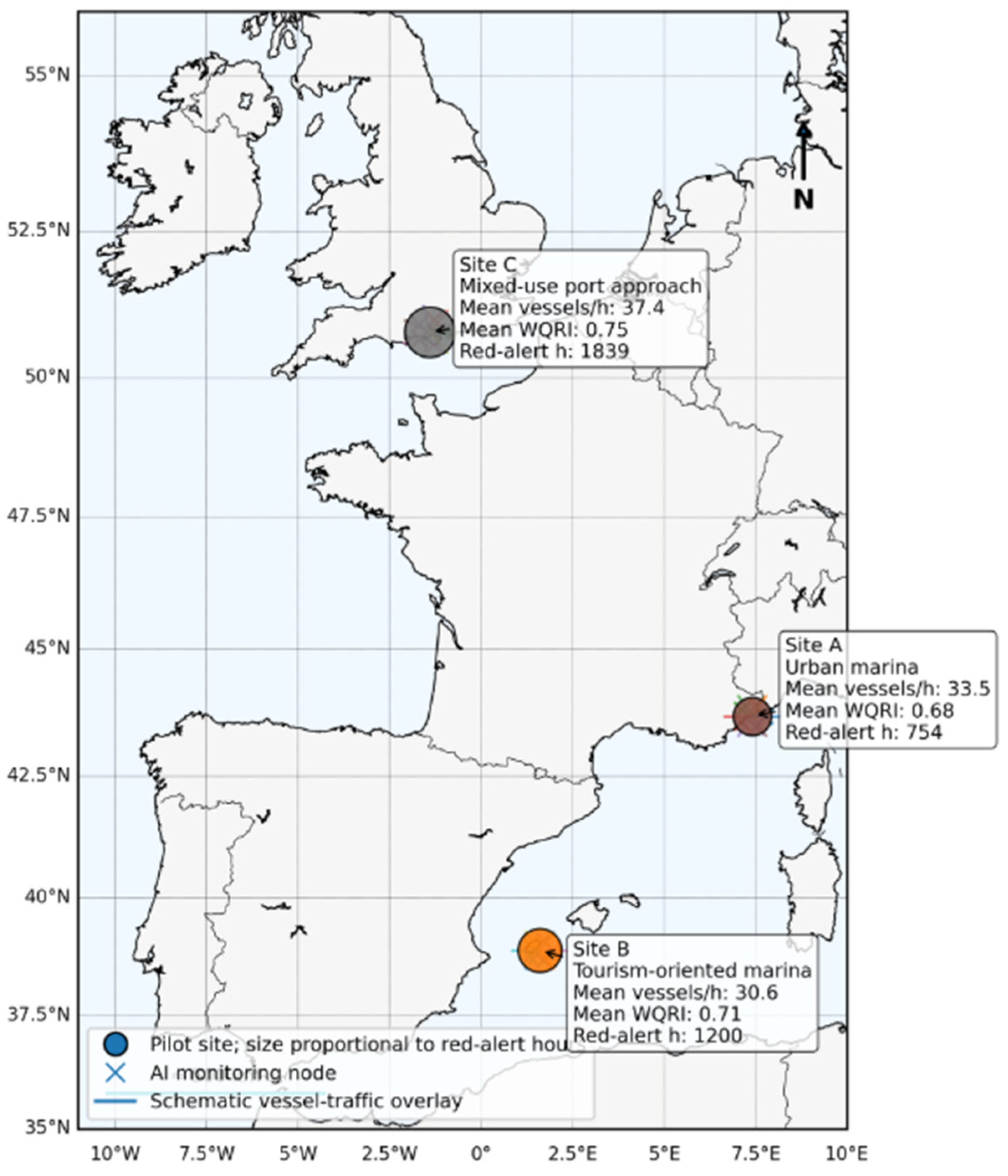
The study employed an observational design without experimental manipulation of vessel traffic or environmental conditions. Data were collected continuously over 90 consecutive days during summer 2025. We chose these three sites (Figure 1) to reflect very different working environments, rather than to create a geographically representative sample of European coastlines [1,3,5,15].

Site A, an urban marina serving mostly local users, experiences predictable vessel traffic dominated by leisure craft, with a smaller number of service and maintenance vessels. Activity holds fairly steady day to day, following tidal and daily patterns. Site B, a tourism marina, supports a more varied mix of vessels, including bareboat charters, visiting yachts, RIB tours, and day-trip passenger vessels. Traffic peaks around arrival and departure periods and varies substantially between weeks in response to weather conditions and the tourism calendar. Site C is a mixed-use port approach channel shared by commercial fishing vessels, small cargo operations, and recreational craft, and has the most operationally complex traffic profile of the three sites [1,3,5].

To make these operational disparities concrete,

Table 1. Comparative operational baseline of the three coastal sites.

Operational Baseline Metric	Site A—Urban Marina [18]	Site B—Tourism Marina [19]	Site C—Mixed-Use Port [20,21]
Total berths/mooring points	~760	~1400 pleasure-boat moorings, port-wide	Multiple marinas; ~3500 recreational vessels licensed harbour-wide, plus a dedicated commercial fishing quay
Indicative navigation duration within harbour (h per vessel movement)	0.25 (author-estimated scenario)	0.35 (author-estimated scenario)	0.50 (author-estimated scenario)
Predominant vessel category	Leisure craft	Charter/RIB tour/day-trip	Commercial fishing/small cargo/recreational
Channel/basin width (m)	~100 (entrance channel)	Not publicly documented (channel depth only: 7.1–9.1 m)	50 (Small Boat Channel)

summarises the physical and operational baseline of each site independently of the environmental monitoring data. This baseline context clarifies why raw vessel counts are not directly comparable across sites without accounting for berth capacity and channel usage.

Berth counts and channel or entrance characteristics are drawn from publicly available marina and harbour authority sources and are included only to indicate the relative scale and typology of the three operational settings [18,19,20,21]. They are not the monitoring observations used to calculate WQRI or train the models. Published navigation-duration observations were unavailable. The values presented in Table 1 are therefore author-estimated scenarios rather than measured means, AIS-derived values or model inputs, and should be interpreted only as indicative operational context.

The scenario values reflect a qualitative assessment of harbour compactness, approach complexity, speed restrictions, tidal effects and traffic control. Because consistent berth-to-boundary route distances were unavailable, these estimates are not presented as reproducible transit-time calculations. No inferential result depends on them.

All three sites have been anonymised. Coordinates, site names, and operator identities have been removed from all datasets and outputs. What is retained is the temporal structure of the monitoring period and the operational typology of each site [4]. The analysis focuses on site type rather than specific geography, which supports the applicability of the observed patterns to comparable sites elsewhere.

2.2. Data Sources and Variable Structure

The study used four categories of variables: vessel traffic, environmental water quality, weather, and operational management responses. Vessel traffic variables were recorded hourly and represented by total vessel count, mean vessel speed, speed variance across vessels in the monitoring zone, berth occupancy as a proportion of total berth capacity, and a near-miss proxy derived from simultaneous arrivals and departures in constrained channel sections. These five variables capture both volume and the behavioural characteristics of traffic that drive physical disturbance. Environmental variables measured continuously at each site included turbidity (NTU), dissolved oxygen (mg L⁻¹), a chlorophyll proxy derived from fluorometric measurements, and water surface temperature (°C) [3,5,6,7,8].

Table 2. Comprehensive summary of vessel traffic, environmental, weather, and operational response variables used to construct the WQRI and to train the two AI layers.

Category	Feature	Description	Unit
Vessel traffic	Total vessel count	Number of vessels present in the monitoring zone	vessels h−1
Vessel traffic	Mean vessel speed	Average speed of vessels in the monitoring zone	kn
Vessel traffic	Vessel speed variance	Variance of vessel speeds across the monitoring zone	kn2
Vessel traffic	Berth occupancy	Occupied berths as a proportion of total berth capacity	proportion (0–1)
Vessel traffic	Near-miss proxy	Simultaneous arrivals/departures in constrained channel sections	count h−1
Environmental	Turbidity	Water column turbidity	NTU
Environmental	Dissolved oxygen	Dissolved oxygen concentration	mg L−1
Environmental	Chlorophyll proxy	Fluorometric proxy for chlorophyll concentration	relative fluorescence units
Environmental	Water surface temperature	Continuous surface water temperature	°C
Weather	Rainfall	Total hourly rainfall	mm h−1
Weather	Wind speed	Mean hourly wind speed	m s−1
Weather	Wind speed variance	Hourly variance of wind speed	(m s−1)2
Weather	Air temperature	Hourly air temperature	°C
Operational response	Monitoring intensification	Logged instance of increased sampling/monitoring frequency	event count
Operational response	Traffic advisory	Logged formal advisory issued to vessel operators	event count
Operational response	Physical inspection	Logged on-site inspection	event count
Operational response	Traffic management intervention	Logged direct traffic management action	event count
Composite index	WQRI	Composite Water Quality Risk Index (weighted sum of five normalised sub-components)	index (0–1)

consolidates all variables used in this study, together with their description and unit of measurement, to give a single reference point for the feature set feeding the WQRI and the two AI layers.

A composite index was chosen over reporting the four environmental signals separately for three practical reasons. First, individual parameters such as turbidity or dissolved oxygen move on different scales and respond to different processes, so watching them side by side does not, on its own, tell a manager whether overall conditions are deteriorating; a single composite score does. Second, a common 0–1 index allows conditions to be compared directly across sites with very different baseline characteristics and across time, which is essential for a system intended to support a regional manager overseeing a portfolio of sites rather than a single location. Third, embedding traffic pressure as one of the five sub-components, alongside the four water-quality signals, keeps the vessel-activity contribution to environmental stress explicit in the index itself, rather than treating traffic purely as an external predictor, which is consistent with the mechanistic link between vessel movements and the other four stressors described above. The trade-off is that a composite index obscures which sub-component is driving a given alert; Section 3 reports feature importance separately to help recover that detail.

The Water Quality Risk Index (WQRI) aggregates these environmental signals into a single composite score. Turbidity disturbance, dissolved oxygen depletion, chlorophyll anomalies, thermal variability, and a traffic pressure term derived from the vessel traffic variables are the five contributing sub-components. Each sub-component was normalised to a 0–1 scale and combined using a weighted scheme:

$$\mathrm{W}\mathrm{Q}\mathrm{R}\mathrm{I}=\sum _{t=1}^n{w}_i.x_i$$

where

• $x_i$ represents normalised environmental variables,
• $w_i$ represents weighting coefficients,
• $\sum w_i=1$.

where x_i is a normalised variable and w_i its weight, with weights summing to 1. The index brings together five distinct stressor signals into a single number that can be tracked across sites and time without re-scaling. We set WQRI ≥ 0.70 as the operational high-risk (red) threshold, and values at or above this threshold indicate high risk and the need for enhanced monitoring and possible intervention. That cut-off was calibrated based on the first 15 days of data at each site rather than imposed from published benchmarks, which would not have accounted for site-specific baseline conditions.

The five sub-components were weighted equally (0.20 each) rather than through an empirically derived scheme. This a priori choice reflected the absence of evidence that any single stressor dominated risk across all three site types during the pilot. The red threshold was fixed at WQRI ≥ 0.70. Amber alerts were derived from each site’s first-15-day WQRI distribution below the red threshold; however, the exact site-specific amber cut-offs were not retained in the analysis record. The binary red versus not-red evaluation is therefore reproducible from the reported threshold, whereas the full three-category interface cannot be independently reconstructed from the available documentation. This limitation is stated explicitly in Section 5.

Weather variables recorded hourly were total rainfall, mean wind speed, wind speed variance, and air temperature. Operational response records were compiled from site management logs throughout the monitoring period. Four response categories were tracked by this study. These were monitoring intensification, formal traffic advisories, physical inspections, and direct traffic management interventions. These response records were included so the study could look at whether alerts led to real management action, rather than just measuring model performance on held-out data [6,7,9,10].

2.3. AI-Enabled Decision Support Framework

At coastal sites, risk tends to emerge from combinations of factors rather than any one variable alone. The same high vessel count means something different on a calm day with good oxygen saturation than it does after two days of heavy rain and strong onshore winds [22]. The system architecture reflects this.

Layer 1 addressed short-term operational risk. Gradient boosting models took as inputs the current hour’s vessel count, mean speed, speed variance, and berth occupancy, together with the previous two hours’ values and concurrent weather measurements for rainfall and wind variability. The output was an estimate of current traffic-related environmental stress which was considered to be fast enough to support decisions about inspection deployment during an active event.

The Layer 1 output is the traffic-pressure sub-component of WQRI (normalised 0–1), estimated hourly from current and short-lag vessel and weather inputs; it is not a separately labelled construct. Both models were fitted to the pooled three-site dataset using an 80/20 split described in the project record as stratified. The models used the implementation’s default settings without a tuned hyperparameter search. The software version, random seed, precise stratification variable, observation counts after preprocessing and detailed missing-data treatment were not retained in the project documentation. These omissions limit exact computational reproducibility and are acknowledged in Section 5.

The predictive function was defined as:

$$\mathrm{F}\left(\mathrm{x}\right)=\sum _{m=1}^M{\gamma }_m.h_m(x)$$

where:

• $h_m\left(x\right)$ represents weak learner decision trees,
• ${\gamma }_m$ represents optimisation weights,
• $M$ represents the number of boosting iterations.

Layer 2 addressed next-day risk prediction. Random forest models took the current WQRI, lagged environmental variable values, the Layer 1 stress estimate, and the preceding 24 h traffic pattern as inputs, producing a predicted risk category for the following day. The risk categories were classified as low, amber, or red. This gives managers enough lead time to position resources ahead of predicted high-risk conditions.

While the model outputs a three-category prediction (low/amber/red) to give managers graded lead-time information, the evaluation reported in Section 3 deliberately collapses this to a binary high-risk versus not-high-risk decision (red versus low + amber), since that is the operationally decisive distinction for triggering inspection and advisory responses: the cost of missing a genuine red-alert event is materially different from misclassifying between the two lower categories. The confusion matrix and ROC curve in Section 3 should therefore be read as evaluating this binary decision layer, not the full three-way classification. This means the model’s ability to distinguish amber from low risk specifically has not been separately validated.

The classification probability function was:

$${\mathrm{P}}_{\left(y\right|x)}={\displaystyle \frac{1}{N}}\sum _{t=1}^N\left({\displaystyle \genfrac{}{}{0pt}{}{n}{k}}\right)T_i(x)$$

where:

• $T_i\left(x\right)$ represents individual decision-tree outputs,
• $N$ represents the total number of trees.

WQRI served as the common risk currency across both layers and all three sites. A single index that means the same thing regardless of site type matters for a system a regional manager might use across a portfolio of sites: they should not need to re-interpret scale at each location.

Amber alerts signalled that conditions were moving in a direction that needed close watching and that staff should be ready to step in if required. Red alerts signalled that conditions had reached a point where direct action was warranted, for example taking water samples, informing vessel operators, or carrying out an on-site inspection. Both alert levels were set using quantiles from the WQRI values observed during the first 15 days, which were treated as a calibration period. The system highlighted situations and suggested types of response, but humans remained in charge throughout. Managers reviewed each alert and decided which specific actions to take [9,10,14,15].

2.4. Statistical Analysis

The statistical analysis followed a single, integrated workflow linking vessel traffic, water quality risk, alert behaviour, and model performance. Hourly vessel counts were first used to calculate WQRI for each observation, and the full 90-day record at each site was summarised with standard descriptive statistics, including mean and peak hourly vessel intensity, mean WQRI, the proportion of hours classified as high-risk, total red-alert duration, and the total number of recorded interventions [3,5,6,7].

To examine how risk changed under different levels of traffic, hourly observations were assigned to five vessel-intensity classes (0–20, 21–30, 31–40, 41–50, and more than 50 vessels per hour), and mean WQRI was calculated within each class for each site. Pearson and Spearman correlation coefficients were then computed between hourly vessel intensity and WQRI at each site: Pearson r was used to quantify linear association, while Spearman rho captured monotonic association without assuming linearity. Where the two coefficients were similar in magnitude, the relationship was treated as approximately linear. Using both measures reduced sensitivity to distributional assumptions and provided a more complete view of the vessel intensity–WQRI relationship [7,8].

Temporal patterns in amber and red alerts were analysed across the 90-day window, with attention to clustering of alerts, the duration of sustained high-risk periods, and alignment with recorded traffic spikes and adverse weather episodes. Cross-site comparisons of all metrics identified differences in risk profiles attributable to site type and operational context and provided evidence for the practical value of the AI-enabled decision-support system [9,10,15]. Finally, the gradient boosting and random forest models were evaluated against held-out data using standard performance metrics, completing the link from observed vessel traffic through WQRI and alert dynamics to AI-supported operational decision-making [6,7].

3. Results

3.1. Site-Level Traffic and Water-Quality Risk Profiles

Table 3. Site-level operational and environmental characteristics during the 90-day monitoring period.

Metric	Site A—Urban Marina	Site B—Tourism Marina	Site C—Mixed-Use Port
Mean vessel intensity (vessels h−1)	30.6	37.4	35.4
Peak vessel count (vessels h−1)	58	71	68
Mean WQRI	0.68	0.71	0.75
Red alert duration (h)	108	170	183
Intervention frequency	12	17	21
Mean rainfall (mm h−1)	0.6	0.4	0.8
Mean wind speed (m s−1)	4.2	3.8	5.1

summarises the key operational and environmental metrics for all three sites across the full monitoring period. Site B recorded the highest mean vessel intensity, at 37.4 vessels h⁻¹, and the highest peak, at 71 vessels h⁻¹. This pattern is consistent with the concentrated arrival-and-departure windows typical of tourism charter operations. Site C averaged 35.4 vessels h⁻¹ and Site A 30.6 vessels h⁻¹ [3,5].

Site C recorded the highest mean WQRI (0.75), accumulated 183 red-alert hours—more than either of the other sites—and required the greatest number of management interventions. Site B had a mean WQRI of 0.71 and Site A 0.68. The contrast between Site B and Site C is the most operationally relevant finding from the descriptive summary: Site B had higher peak vessel counts, but Site C had higher sustained water quality risk. Persistence of moderate-to-high traffic levels through the day, rather than brief extreme peaks, appears to drive greater cumulative environmental pressure [6,7,8,9,10,15].

These results show that risk did not correspond to vessel volume in a simple linear manner. Site C was busier than Site A but not by much; what set it apart was the mix of vessel types and the unrelenting nature of its traffic through the day, which translated into substantially longer periods of elevated WQRI. Operational context, and not just throughput, is what determined the environmental risk profile.

3.2. Environmental Risk Under Different Vessel Intensity Classes

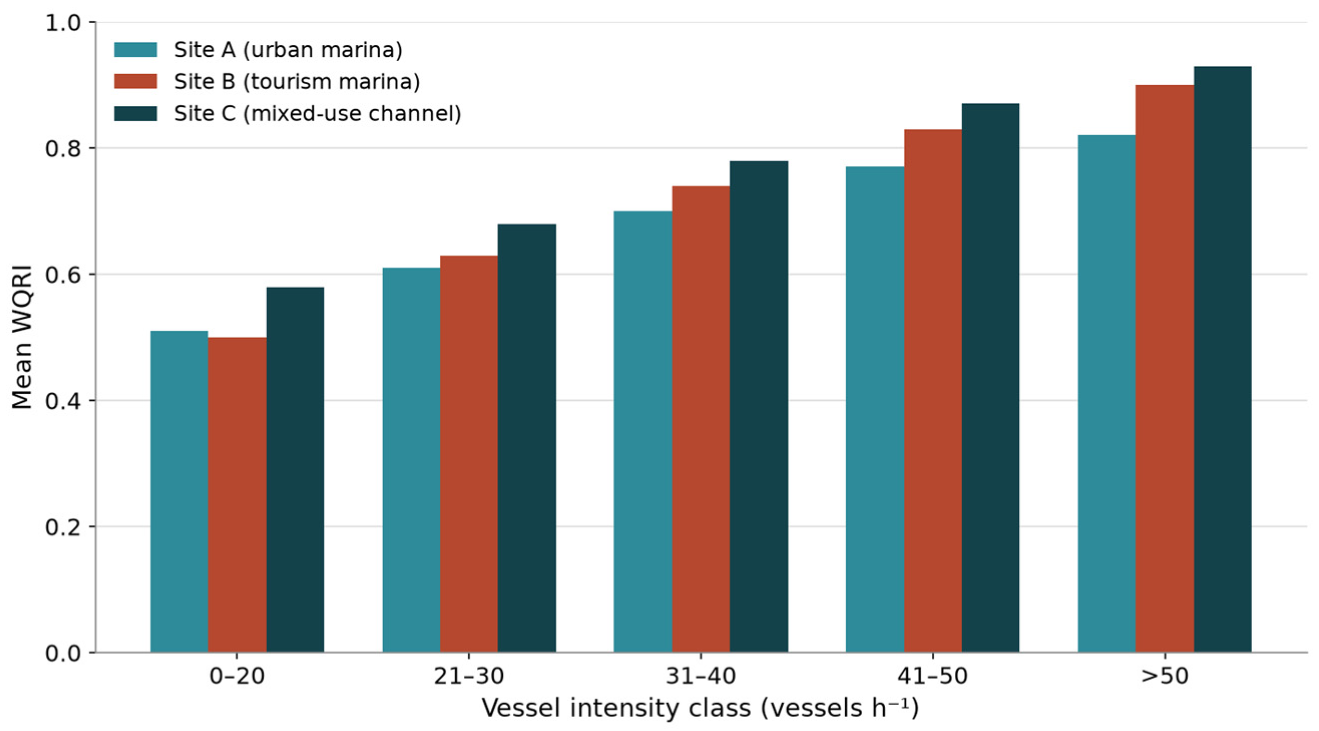
Figure 2 and

Table 4. Mean Water Quality Risk Index (WQRI) values across vessel intensity classes for each coastal typology.

Vessel Intensity Class (Vessels h−1)	Site A	Site B	Site C
0–20	0.54	0.52	0.61
21–30	0.63	0.65	0.71
31–40	0.71	0.74	0.77
41–50	0.77	0.82	0.85
>50	0.84	0.92	0.94

show WQRI as a function of vessel intensity class across all three sites. At every site, mean WQRI rose progressively from the lowest to the highest intensity class, confirming that the association between traffic volume and water quality risk is consistent and directional rather than threshold-dependent. Site B showed the sharpest rate of increase: mean WQRI moved from 0.50 at the 0–20 vessel intensity class to 0.90 at the greater-than-50 class. Site C tracked the highest absolute values throughout the range, from 0.58 at the lowest class to 0.93 at the highest. Site A rose from 0.51 to 0.82, a more gradual gradient. This is consistent with earlier studies showing that vessel traffic affects coastal water quality through disturbance, pollutant loading, and sediment resuspension [3,5,6,7].

3.3. Correlation and Association Between Vessel Activity and Environmental Risk

Table 5. Correlation coefficients describing the relationship between vessel intensity and WQRI.

Site	Pearson r	Spearman ρ
Site A (Urban Marina)	0.61	0.58
Site B (Tourism Marina)	0.70	0.67
Site C (Mixed-Use Port)	0.66	0.64

gives the Pearson and Spearman coefficients for each site. All coefficients were positive and statistically significant. Site B showed the strongest association: r = 0.701, rho = 0.672. The other two sites sat in the moderate-to-strong range. Across all three, the two coefficients were similar, indicating that the relationship between vessel count and WQRI is approximately linear, not just monotonic, so vessel count can go directly into a risk model as a predictor without transformation [6,7,8].

One caveat applies to this correlation and to Figure 2 and Table 4 more broadly: traffic pressure is itself one of the five sub-components used to compute WQRI, so part of the observed association between vessel intensity and WQRI is built into the index definition rather than being a fully independent empirical finding. The correlation is not purely circular, since WQRI also incorporates four environmental signals that are not deterministic functions of vessel count, but the reported coefficients should be interpreted as an upper bound on the true strength of the traffic–risk relationship rather than as an estimate obtained from fully independent measures.

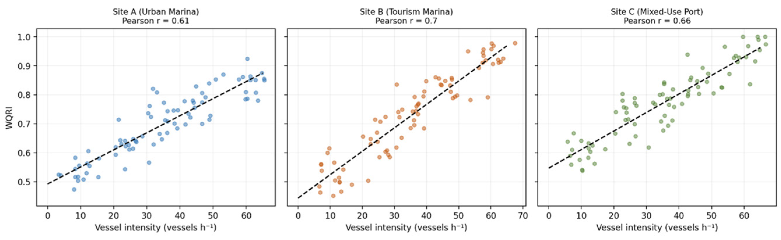
At all three sites, Pearson and Spearman values were close in magnitude (Table 5). This convergence indicates that the relationship between vessel intensity and WQRI is not only monotonic but approximately linear across the observed intensity range (Figure 3). This is a useful property because it means vessel count can serve as a direct predictor in a linear modelling context without requiring transformation. Vessel traffic data, already routinely collected at most managed marinas and ports, can therefore function as a meaningful proxy for real-time water quality risk [6,7,8].

3.4. Temporal Risk Behaviour and Alert Patterns

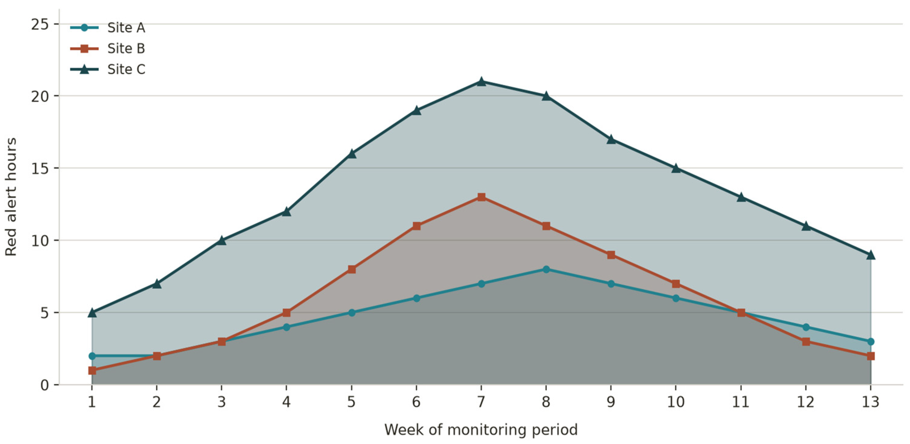
Elevated-risk periods recurred throughout the 90-day monitoring window at all three sites (Figure 4). Amber-level alerts were more frequent than red alerts at every site, consistent with a pattern of regularly elevated conditions punctuated by fewer, more severe events. Site C exhibited the most sustained red alert periods: on several occasions red alert conditions persisted for blocks of consecutive hours rather than appearing as isolated spikes.

Risk elevations were rarely attributable to traffic alone or weather alone. The sharpest WQRI exceedances corresponded to periods when high vessel activity coincided with adverse weather, specifically strong onshore winds and elevated rainfall in the preceding 12 h. WQRI responses were more moderate when only one of the two factors was present. This matters for threshold design, since a model that treats weather and traffic independently will understate their combined effect when both occur at once [9,10].

3.5. AI Model Performance and Decision Support Outcomes

On the held-out test set, the Layer 1 gradient boosting model achieved R² = 0.82, RMSE = 0.071, and MAE = 0.054 for the estimation of hourly traffic-related environmental stress, using an 80/20 train–test split. A full scatter plot of predicted versus observed test-set values is not included; only the summary regression metrics above are reported.

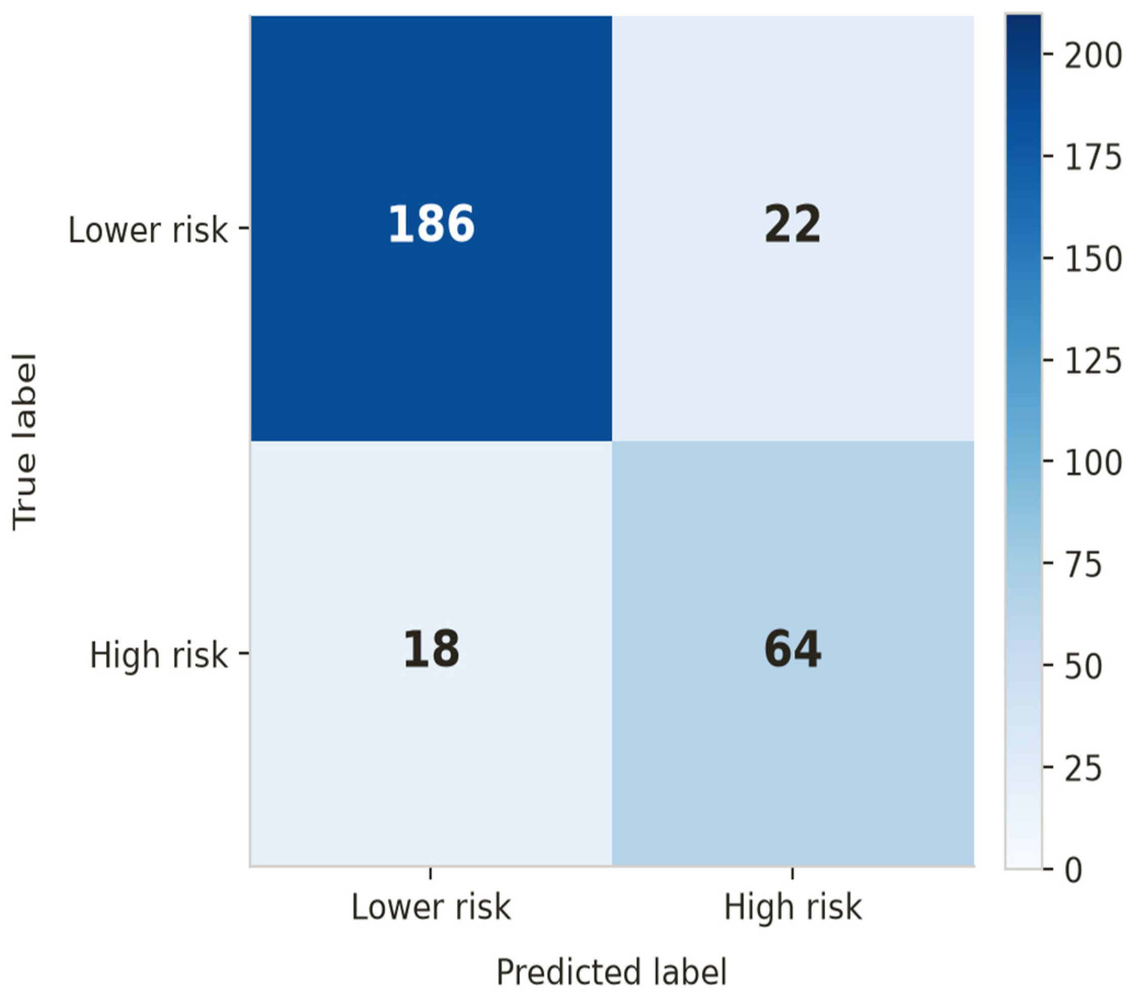
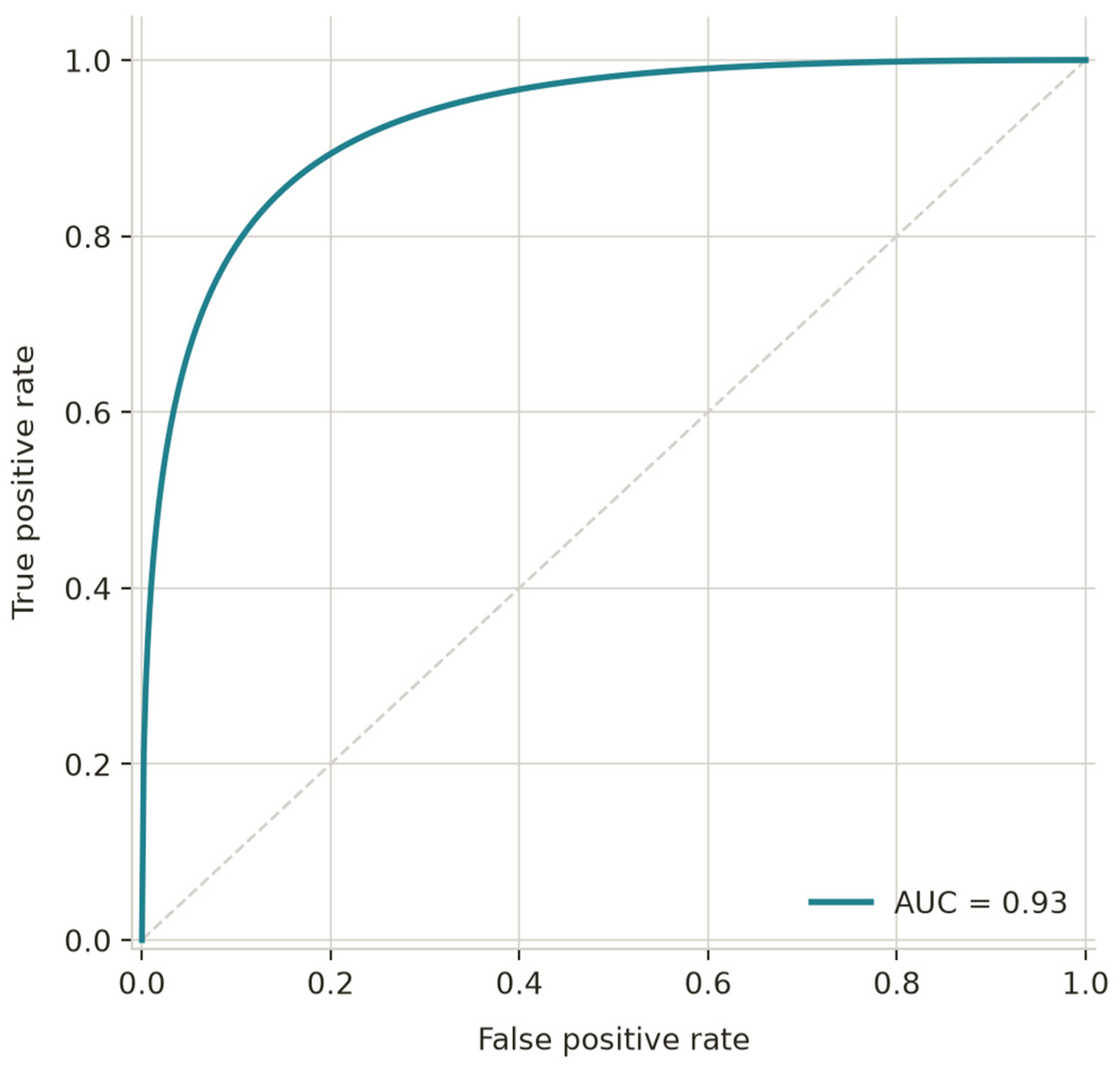
The random forest model (Figure 5), developed to predict next-day risk, achieved an overall accuracy of 86.2% on the held-out test data. Precision, recall and F1 score were each 0.87, and the AUC was 0.93 (

Table 6. Performance metrics of the random forest environmental risk classifier.

Metric	Value
Accuracy	0.862
Precision	0.87
Recall	0.87
F1 Score	0.87
AUC	0.93

). The confusion matrix showed a broadly balanced distribution of false-positive and false-negative classifications for the binary high-risk versus not-high-risk decision.

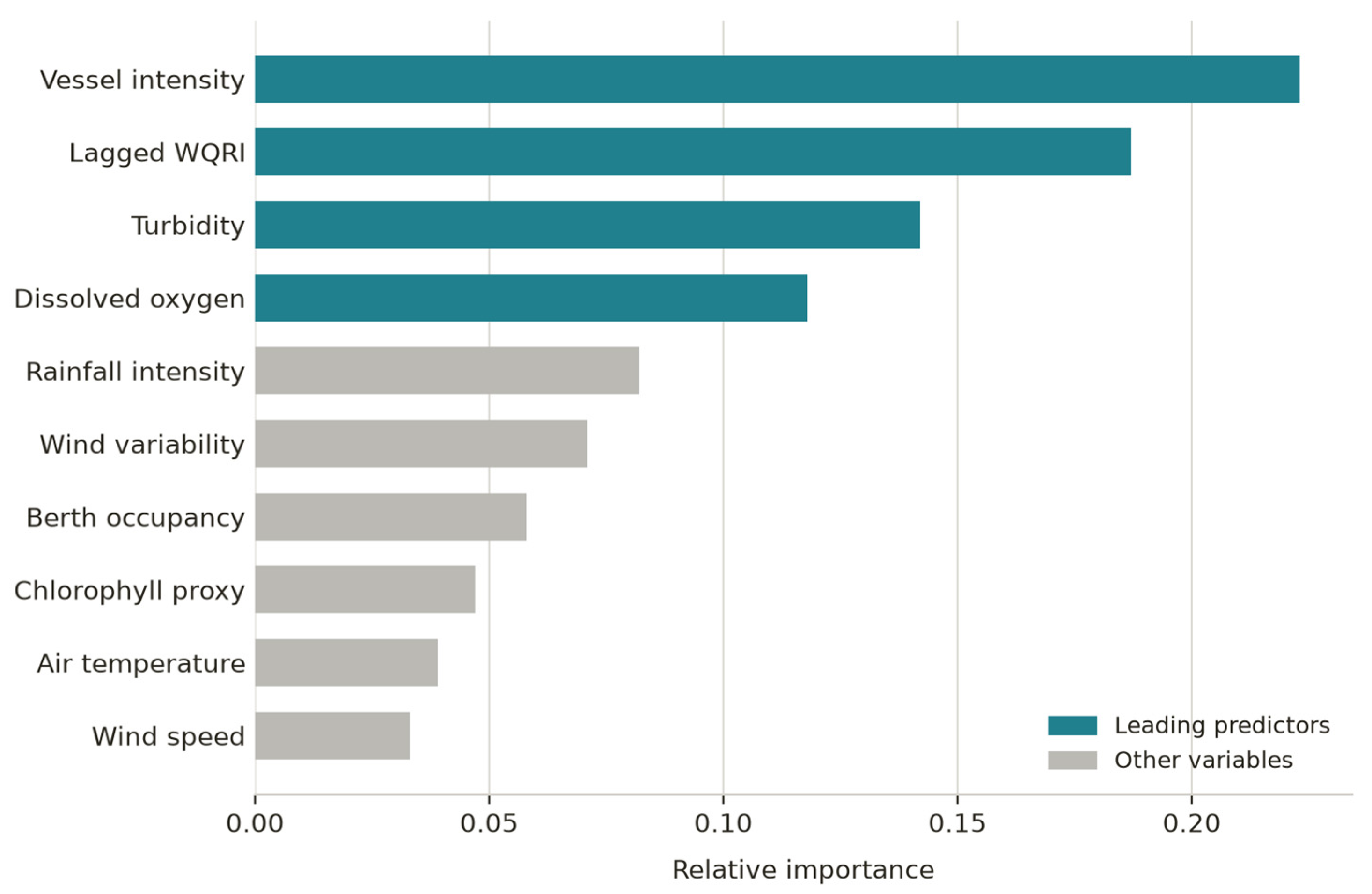
Four variables emerged as the most influential predictors: vessel intensity, lagged WQRI, turbidity and dissolved oxygen. This pattern is consistent with established mechanisms: vessel movements resuspend sediments and increase turbidity, while associated organic loading may reduce dissolved-oxygen concentrations. Lagged WQRI was also influential because recovery from a disturbance is not immediate [9,10,15].

Over the 90-day period, the amber/red structure converted continuous sensor measurements into a limited number of operational categories. Managers were not required to interpret continuous streams of raw turbidity or dissolved-oxygen data; instead, each alert indicated whether a response was warranted and guided the type of response. The deployment of inspections, advisories and traffic-management measures following specific alerts provides practical evidence that the outputs were considered sufficiently credible to inform decisions [9,10,15].

Figure 6 shows the ROC curve for the Random Forest classifier. With an AUC of 0.93, the model demonstrates strong discrimination between lower-risk from high-risk conditions across thresholds—the curve sits well above the dashed diagonal, which marks the performance of a classifier making random guesses.

These results align with the model’s overall accuracy of 86.2%. Accuracy reflects performance at a single threshold, whereas the AUC of 0.93 shows this performance holds across a range of thresholds. The relatively balanced error rate (22 false positives, 18 false negatives) further indicates that the classifier performs consistently rather than favouring one type of error.

The classifier is not compared here against a simple non-ML baseline, such as WQRI persistence (i.e., predicting tomorrow’s risk class from today’s mapped class). While the random forest’s 86.2% accuracy and 0.93 AUC indicate strong absolute performance, the added value of the machine-learning layer over the simplest possible operational heuristic has not yet been quantified. Closing this gap is a priority for the next phase of this study.

4. Discussion

Water quality risk, as measured by WQRI, rose with vessel intensity at all three sites. The present study provides quantitative evidence through correlation coefficients, intensity-class gradients, and a 90-day time series that put numbers on a relationship previously assumed rather than measured at this temporal resolution [3,5,6].

Comparison of Sites B and C showed that Site B recorded the higher peak vessel count (71 vessels h⁻¹), whereas Site C exhibited the higher mean WQRI and more red-alert hours. Site C experienced sustained moderate-to-high throughput across commercial and recreational vessel types, rather than concentrated short-duration peaks. This pattern suggests that the duration of traffic pressure may be more important than peak intensity for cumulative water-quality deterioration. However, because site type and vessel composition are confounded with traffic duration, this interpretation should be tested through within-site and multi-season analyses [7,8].

The Pearson–Spearman convergence across all three sites supports using vessel count as a direct, low-cost risk proxy. Most coastal facilities with vessel monitoring systems already log vessel counts automatically. Feeding that data into a risk scoring system requires no additional sensor investment. The marginal cost of the monitoring layer is essentially the computational infrastructure to run the model, not new measurement equipment. This matters for adoption, especially at sites where environmental monitoring budgets are tight [6,7,8].

Previous AI applications to coastal and marine environments have predominantly focused on the prediction step. Bellou et al. [1], Ning et al. [9], and Prakash and Zielinski [10] each demonstrated that ML models can predict conditions of interest with useful accuracy. The contribution of the present study is to extend prediction into prescribed operational action. The WQRI threshold triggers an amber or red alert, and that alert category specifies what the manager should do next, for example intensify sampling, issue a vessel advisory, or deploy an inspector. The distinction between ‘risk is elevated’ and ‘do this now’ separates information from decision support. Alotaibi and Nassif [11] identified this gap in their survey of AI ocean monitoring tools and the system described in this study is a direct attempt to close it.

The random forest AUC of 0.93 is high for a field-deployed model operating across diverse site types with no model-specific tuning between sites. The four leading predictors correspond directly to established mechanisms of vessel-driven water quality degradation: vessel intensity initiates sediment resuspension and organic enrichment, while the lagged WQRI captures the multi-hour recovery deficit that follows high-traffic periods (Figure 7). This physically grounded predictor hierarchy supports the explainability of model outputs and reduces the specialist knowledge required for managers to interpret and act on individual alert events.

Human oversight was incorporated deliberately because automatic responses to model outputs would be legally and operationally inappropriate in most marine permitting contexts. A vessel operator cannot be denied berth access solely on the basis of an algorithmic output. That decision remains with the harbour master, who may use the alert as supporting evidence. The transparent amber/red threshold structure also enables managers to explain why an alert was generated and to override it when local evidence contradicts the model prediction [9,10,14,15].

SDG 14 asks member states to reduce marine pollution and demonstrate progress. Demonstrating such progress is particularly challenging at sites operating with limited environmental monitoring capacity. A continuously operating monitoring architecture that autonomously identifies risk and produces a timestamped audit trail of each alert and corresponding response reconceptualises compliance from a periodic, calendar-driven obligation into a form of ongoing stewardship, leveraging data infrastructures that are already embedded in most port and marina environments. The European Commission’s ocean policy targets, which require evidence of measurable pollution reduction [23,24], are precisely the kind of reporting context this kind of system was designed to feed.

A related interpretive caveat concerns how WQRI itself is constructed. Because the five sub-components were weighted equally rather than through an empirically derived scheme, the composite index reflects an a priori judgement that no single stressor dominates risk, not a data-driven weighting decision, and this subjective choice has real interpretive consequences for the findings reported above: differences in mean WQRI across sites and vessel-intensity classes partly reflect the fixed weighting itself rather than purely independent site-level differences in the underlying stressors, and a site whose true dominant stressor differs from the assumed equal weighting could show a WQRI value that misrepresents its actual risk profile even where individual sensor readings are accurate. We treat this as a substantive limitation rather than a presentational detail and see resolving it as the most important methodological priority for follow-up work. Objective alternatives include principal component or factor analysis to derive data-driven weights, supervised weight optimisation against an independent validation outcome, structured multi-rater expert elicitation, and systematic sensitivity analysis across alternative weighting schemes to establish how robust the reported site rankings and traffic–risk relationships are to the weighting choice; we return to these options in Section 5.

5. Limitations

The study’s scope points to several areas where further work would add robustness rather than undermining the current proof of concept.

The monitoring covered a single 90-day summer window at three sites, so temporal and spatial generalisability to other seasons, years, and coastal typologies remains to be established. The WQRI weighting scheme and pollutant coverage were tailored to the specific marina settings and variables observed; applications in different environments will require recalibration of component weights and extension to additional pollutant classes (for example, nutrients, faecal indicators, hydrocarbons, and microplastics).

The five WQRI sub-components were also weighted equally rather than estimated from data, an a priori choice made because no single stressor was assumed to dominate risk at the pilot stage. This is a genuine limitation rather than a neutral default: a site where the true dominant stressor differs from the assumed weighting could show a WQRI that misrepresents local risk even with accurate sensor data, and the vessel intensity–WQRI correlation reported in Section 3 is itself partly a consequence of this fixed weighting rather than a purely independent empirical finding. Objective alternatives for follow-up work include principal component or factor analysis, supervised weight optimisation against an independent validation outcome, structured multi-rater expert elicitation, and sensitivity analysis across alternative weighting schemes; resolving this is, in our assessment, the most important methodological priority for future WQRI-based systems.

Table 1’s mean daily vessel navigation duration figures carry a related limitation: this metric is not published for any of the three site types, so the values shown (0.25–0.50 h) are estimated from published speed limits and harbour geometry rather than AIS-derived observed means, and were not used in the WQRI computation, model training, or any reported result.

The evaluation reported in this pilot is narrower than a full validation study. The exact site-specific amber thresholds were not retained, so only the binary red versus not-red decision is fully reproducible. The classifier was not benchmarked against WQRI persistence; Figure 2 lacks within-class dispersion; Figure 6 provides no site-specific ROC curves; and Layer 1 is reported without a predicted-versus-observed plot. In addition, the software version, random seed, split-stratification variable and preprocessing details were not retained. These gaps restrict reproducibility and prevent firm conclusions about improvement over a simple operational baseline or consistency across sites. They define the minimum analysis and documentation requirements for follow-up validation.

The machine-learning models were trained on this 90-day dataset, and their performance under unobserved or extreme conditions (such as major storms, accidental fuel releases, or bloom-favourable calm periods) is not yet known, underscoring the value of multi-year training records. Finally, the analysis is correlational: vessel activity shows a strong association with WQRI, but other co-varying drivers (tidal state, wind, rainfall, sediment resuspension) were not disentangled, and hydrodynamic processes were not explicitly modelled. Incorporating hydrodynamic modelling and longer, more diverse datasets would enable stronger causal inference and more transferable risk thresholds.

This pilot has not been benchmarked against long-term regional climatology, so we cannot state whether summer 2025 was climatologically typical, unusually calm, or unusually stormy at the three sites; the model’s behaviour under different seasonal weather regimes is accordingly unknown and is treated as part of the generalisability limitation above. Relatedly, the duration-versus-peak comparison between Site B and Site C is a three-site, one-summer observation rather than a controlled test: Site C’s port-approach setting combines commercial fishing and cargo traffic with pollution sources (bottom disturbance from trawling, bilge discharge, differing fuel types) that differ materially from the recreational craft dominant at Site B, so site type and vessel type are confounded with traffic duration in this comparison. A within-site analysis comparing weeks of sustained moderate traffic against weeks of spikier traffic at the same site would test the duration hypothesis more directly, and we identify this, together with the seasonal-representativeness question above, as priorities for the follow-up validation study.

Implications for Marine Pollution Assessment and Solutions

The standard approach to environmental monitoring in marinas and small ports follows a fixed timetable, such as fortnightly water sampling, monthly visual surveys and annual compliance reporting. This schedule may bear little relationship to recent operational conditions, including vessel arrivals, stormwater runoff or prolonged periods of reduced tidal exchange. A risk-triggered approach instead directs monitoring resources towards locations and periods in which the model indicates deteriorating conditions. Such an approach could increase the probability that inspections coincide with short-duration exceedances.

Vessel tracking data is already collected as a matter of routine maritime safety and harbour administration. Most marinas and commercial port authorities log arrivals, departures, and vessel movements as standard practice. Feeding that existing data stream into a WQRI calculation requires no new sensor deployment and no change to vessel operator behaviour. Port authorities and marina operators seeking to improve environmental monitoring capability can do so by connecting data systems that already exist, rather than building new infrastructure.

The amber/red alert output also creates a documented decision trail. When a manager receives a red alert and deploys an inspector, the record shows model output at time T, alert generated, inspection authorised and conducted. When that inspection finds an exceedance, the chain of evidence from risk signal to management response to documented finding is complete; when it finds nothing unusual, that result feeds back into model calibration. Regulators increasingly expect this kind of traceable, timestamped record from environmental management programmes, and the alert framework generates it as a by-product of normal operation.

At a policy level, resource-constrained environmental agencies managing multiple coastal sites across a region could use a network of WQRI-enabled sites to allocate limited inspection capacity where and when risk is highest, triaging based on real-time risk scores rather than rotating inspections evenly across a portfolio. That kind of spatially differentiated, risk-responsive allocation is what EU Ocean Mission objectives and SDG 14 targets require from member state monitoring programmes [16,23].

The role of AI in this system is specific and bounded. It does not replace environmental expertise or eliminate the need for trained inspectors. It takes data that already exists, combines it faster and more consistently than a human analyst could across multiple concurrent data streams, and surfaces a risk classification that helps managers prioritise their attention. Expertise still drives the response; the model accelerates the recognition that a response is needed [12].

6. Conclusions

Coastal pollution management has predominantly been retrospective: monitoring records conditions after they change, sampling is conducted post hoc, and interventions follow rather than anticipate disturbance. This study examined whether that sequence is necessary given the temporal dynamics of traffic-driven pollution.

Across three operationally distinct sites, vessel traffic intensity was a consistent predictor of water quality risk as quantified by WQRI. The mixed-use port channel (Site C), characterised by sustained moderate traffic rather than sharp peaks, exhibited the highest mean WQRI and the greatest number of red-alert hours despite lower peak vessel counts than Site B. This pattern suggests that, in mixed-use environments with continuous commercial and recreational activity, the duration of moderate pressure is more influential than peak throughput.

The random forest classifier achieved strong discriminative performance (AUC 0.93). The four dominant predictors—vessel intensity, lagged WQRI, turbidity, and dissolved oxygen—align with established mechanisms of traffic-related water quality degradation, including sediment resuspension, organic loading, and oxygen depletion that persists beyond individual traffic events. The resulting importance structure is sufficiently transparent to support managerial interpretation and justification of alerts without specialist expertise in machine learning.

The system adopts an explicitly human-in-the-loop configuration. In regulated marine contexts, fully automated decision-making is currently inappropriate on operational, legal, and legitimacy grounds. The architecture is therefore designed to enhance the timeliness and resolution of information available to managers while preserving human responsibility for operational decisions.

Overall, the integration of routine vessel tracking, real-time environmental sensing, and supervised risk classification demonstrates that coastal pollution management can move beyond predominantly monthly, retrospective reporting toward more continuous, risk-aware operations. As coastal use intensifies, the empirical and policy case for such a transition is increasingly compelling [11,12,16].

Beyond these site-specific empirical results, the study’s broader contribution is architectural: it demonstrates that an interpretable, two-layer early-warning design, short-horizon gradient boosting feeding a next-day random forest classifier over a shared, index-based risk currency, can convert heterogeneous, multi-source coastal data into a decision-traceable output without requiring black-box modelling. Three points generalise beyond the three pilot sites. First, decomposing risk into a fast operational layer and a slower planning layer addresses two different management timescales with two purpose-built models, rather than forcing a single model to serve both; this decomposition is transferable to other coastal or environmental early-warning problems with similarly layered decision needs. Second, expressing risk through a single normalised composite index rather than raw sensor values allows one classifier architecture to be reused across operationally dissimilar sites without site-specific retuning, which is a reusable design principle for portfolio-level environmental monitoring, subject to the WQRI weighting caveats discussed above. Third, tying model output to a documented amber/red action protocol operationalises explainable AI, not as a post hoc feature-importance exercise alone, but as a structural property of the decision pipeline, since every alert is traceable to a specific WQRI value, threshold, and permitted management response. Together these findings suggest that the value of AI-enabled coastal monitoring lies less in marginal gains in predictive accuracy and more in how prediction, index design, and operational protocol are integrated into a single auditable workflow.

References

- Bellou, N.; Gambardella, C.; Karantzalos, K.; Monteiro, J.; Canning-Clode, J.; Kemna, S.; Arrieta-Giron, C.A.; Lemmen, C. Global assessment of innovative solutions to tackle marine litter. Nat. Sustain. 2021, 4, 516–524. [Google Scholar] [CrossRef] [Scilit]
- United Nations Environment Programme (UNEP). From Pollution to Solution: A Global Assessment of Marine Litter and Plastic Pollution; UNEP: Nairobi, Kenya, 2021. [Google Scholar]
- Blight, L.K.; Bertram, D.F.; O’Hara, P.D. Visual surveys provide baseline data on small vessel traffic and waterbirds in a coastal protected area. PLoS ONE 2023, 18, e0283791. [Google Scholar] [CrossRef] [Scilit] [PubMed]
- European Environment Agency. The European Environment: State and Outlook 2020—Marine Environment Assessment; European Environment Agency: Copenhagen, Denmark, 2019.
- Moore, T.J.; Redfern, J.V.; Carver, M.; Hastings, S.P.; Adams, J.D.; Silber, G.K. Exploring ship traffic variability off California. Ocean Coast. Manag. 2018, 163, 515–527. [Google Scholar] [CrossRef] [Scilit]
- Deng, T.; Chau, K.W.; Duan, H.F. Machine learning based marine water quality prediction for coastal hydro-environment management. J. Environ. Manag. 2021, 284, 112051. [Google Scholar] [CrossRef] [Scilit] [PubMed]
- Grbčić, L.; Družeta, S.; Mauša, G.; Lipić, T.; Vukić Lušić, D.; Alvir, M.; Lučin, I.; Sikirica, A.; Davidović, D.; Travaš, V.; et al. Coastal water quality prediction based on machine learning with feature interpretation and spatio-temporal analysis. Environ. Model. Softw. 2022, 155, 105458. [Google Scholar] [CrossRef] [Scilit]
- Lin, J.; Liu, Q.; Song, Y.; Liu, J.; Yin, Y.; Hall, N. Temporal prediction of coastal water quality based on environmental factors with machine learning. J. Mar. Sci. Eng. 2023, 11, 1608. [Google Scholar] [CrossRef] [Scilit]
- Ning, J.; Pang, S.; Arifin, Z.; Zhang, Y.; Epa, U.P.K.; Qu, M.; Zhao, J.; Zhen, F.; Chowdhury, A.; Guo, R.; et al. The diversity of artificial intelligence applications in marine pollution: A systematic literature review. J. Mar. Sci. Eng. 2024, 12, 1181. [Google Scholar] [CrossRef] [Scilit]
- Prakash, N.; Zielinski, O. AI enhanced real time monitoring of marine pollution: Part 1—A state of the art and scoping review. Front. Mar. Sci. 2025, 12, 1486615. [Google Scholar] [CrossRef] [Scilit]
- Alotaibi, E.; Nassif, N. Artificial intelligence in environmental monitoring: In-depth analysis. Discov. Artif. Intell. 2024, 4, 84. [Google Scholar] [CrossRef] [Scilit]
- Ditria, E.M.; Buelow, C.A.; Gonzalez-Rivero, M.; Connolly, R.M. Artificial intelligence and automated monitoring for assisting conservation of marine ecosystems: A perspective. Front. Mar. Sci. 2022, 9, 918104. [Google Scholar] [CrossRef] [Scilit]
- LeCun, Y.; Bengio, Y.; Hinton, G. Deep learning. Nature 2015, 521, 436–444. [Google Scholar] [CrossRef] [Scilit] [PubMed]
- Liu, P.; Huang, F.; Zarillo, G. New artificial intelligence methods for remote sensing monitoring of coastal cities and environment. Front. Environ. Sci. 2026, 14, 1837937. [Google Scholar] [CrossRef] [Scilit]
- Ioraș, F.; Bandara, I. Artificial Intelligence and Sustainable Practices in Coastal Marinas: A Comparative Study of Monaco and Ibiza. Sustainability 2025, 17, 7404. [Google Scholar] [CrossRef] [Scilit]
- United Nations. Sustainable Development Goal 14: Conserve and Sustainably Use the Oceans, Seas and Marine Resources for Sustainable Development. United Nations Sustainable Development Goals. Available online: https://www.un.org/sustainabledevelopment/oceans/ (accessed on 23 June 2026).
- UNESCO. The United Nations Decade of Ocean Science for Sustainable Development (2021–2030): Implementation Plan; UNESCO: Paris, France, 2021. [Google Scholar]
- Société d’Exploitation des Ports de Monaco. Port Hercule: Berths, Dimensions and Services. Available online: https://www.ports-monaco.com/en/the-ports-of-monaco/port-hercule/ (accessed on 18 July 2026).
- Port Authority of the Balearic Islands (Ports de Balears). Ibiza: Port Overview and Mooring Capacity. Available online: https://www.portsdebalears.com/en/ibiza (accessed on 18 July 2026).
- King’s Harbour Master Portsmouth, Royal Navy. Portsmouth Harbour Entrance, Approach Channel and Small Boat Channel: General Directions. Available online: https://www.royalnavy.mod.uk/khm/portsmouth (accessed on 18 July 2026).
- Metalship. Discover Portsmouth Harbour. Available online: https://www.metalship.org/article/portsmouth-harbour (accessed on 18 July 2026).
- Girau, R.; Anedda, M.; Fadda, M.; Farina, M.; Floris, A.; Sole, M.; Giusto, D. Coastal monitoring system based on social Internet of Things platform. IEEE Internet Things J. 2019, 7, 1260–1272. [Google Scholar] [CrossRef] [Scilit]
- European Commission. Mission Restore Our Ocean and Waters: Implementation Plan 2021–2030; European Commission: Brussels, Belgium, 2021; p. 53.
- European Commission. EU Mission Restore Our Ocean and Waters Progress Report; European Commission: Brussels, Belgium, 2023; p. 283.
Figure 1.
Al-enabled coastal pilot sites for marine pollution decision support.
Figure 2.
Relationship between vessel intensity class (vessels h−1) and mean Water Quality Risk Index (WQRI) across the three coastal typologies. Mean WQRI increased progressively with vessel intensity at all sites. Site B showed the sharpest rate of increase, Site C the highest absolute values throughout the range, and Site A the most gradual gradient. This figure presents class means only; within-class dispersion (e.g., ±1 SD) is not shown, as the underlying per-observation WQRI values are not reported at this level of granularity.
Figure 3.
Scatterplots illustrating the relationship between vessel intensity (vessels h−1) and Water Quality Risk Index (WQRI) across the three coastal typologies. The fitted regression lines show positive traffic–risk relationships at all sites. Site B exhibited the strongest association between increasing vessel activity and environmental risk, whereas Site C maintained comparatively higher WQRI values across the observed range of vessel intensities. Shaded bands represent the uncertainty around the fitted regression relationships.
Figure 4.
Weekly variation in red alert hours across the three coastal typologies over the 90-day monitoring period. Site C saw the heaviest and most sustained red alert burden, peaking sharply around the midpoint of the monitoring period. Site B followed a similar temporal pattern but with a lower peak, consistent with the seasonal concentration of tourism-related vessel activity, whereas Site A maintained comparatively fewer red alert hours throughout the study.
Figure 5.
Confusion matrix for the Random Forest classifier used to distinguish lower- and high-risk environmental conditions. The model correctly classified 186 lower-risk and 64 high-risk observations, while 22 lower-risk observations were classified as high risk and 18 high-risk observations were classified as lower risk. The resulting overall classification accuracy was 86.2% (precision 0.87, recall 0.87, F1 0.87, AUC 0.93).
Figure 6.
Receiver Operating Characteristic (ROC) curve for the random forest environmental risk classifier. This figure presents the pooled ROC curve across all three sites; site-specific ROC breakdowns are not included, so it has not been separately verified whether discriminative performance is consistent across site types or driven disproportionately by one site; this remains a direction for follow-up analysis.
Figure 7.
Relative feature importance scores for environmental risk prediction derived from the random forest classifier. Vessel intensity was the strongest predictor, followed by lagged WQRI, turbidity, and dissolved oxygen. Meteorological variables contributed moderately; berth occupancy and the chlorophyll proxy provided additional smaller predictive value.