Green Growth and the Persistence of Severe Food Insecurity: Temporal Dynamics and Income-Level Heterogeneity in 78 Countries, 2010–2024

Abstract

Severe food insecurity, the level of the Food Insecurity Experience Scale at which people go an entire day without eating, remains above pre-pandemic levels: in 2024, 673 million people (8.2% of the global population) faced hunger and 2.3 billion experienced moderate or severe food insecurity. We examine whether progress in green growth is associated with reductions in severe food insecurity, and over what horizon, using a balanced panel of 78 countries from 2010 to 2024. A dynamic autoregressive model with two-way fixed effects and Driscoll-Kraay standard errors introduces the four dimensions of the Global Green Growth Index (GGGI) as lagged predictors at one, two, and three years. Severe food insecurity is highly persistent: the autoregressive coefficient is 0.941, implying a half-life of at least 11.4 years, and a bias-corrected estimate of 0.970 suggests even greater inertia. Associations with green growth emerge with a delay: Green Economic Opportunities after two years, Efficient and Sustainable Resource Use after three years, while Natural Capital Protection displays a short-run adverse association that dissipates by the third year. Heterogeneity across income levels is confirmed formally, and the protective association of Social Inclusion is confined to low-income countries.

1. Introduction

Severe food insecurity is defined as an inability to access adequate food to the point of going a day or more without eating. In 2024, 673 million people faced hunger, and 2.3 billion experienced moderate or severe food insecurity, 336 million more than before the pandemic [1]. Severe food insecurity remains above pre-pandemic levels despite substantial policy commitment to sustainable development. The COVID-19 pandemic, recurring climate shocks, and commodity price volatility compounded structural deficits in food systems, particularly in Sub-Saharan Africa and South Asia.

Much of the debate on development policies is based on the premise that green growth strategies, investments in social inclusion, protection of natural capital, green economic opportunities, and efficient resource use can simultaneously reduce food insecurity and limit environmental degradation [2,3]. The Global Green Growth Index (GGGI) operationalizes this premise through four composite dimensions that measure countries’ progress along each of these policy fronts. However, empirical evidence on whether improvements in the GGGI dimensions reduce food insecurity remains controversial, with some studies finding no effect as frequently as beneficial effects [4].

Regarding the efficient and sustainable use of resources, this implies optimizing economic value while minimizing environmental impact. It is a circular model that ensures the conservation of raw materials, arable land, energy, and water, rather than simply extending their use to the maximum. The three main concepts considered in this approach are: (1) prioritizing reduced consumption, reusing items to extend their life cycle, and recycling materials to conserve virgin resources, arable land, and energy; (2) designing products and processes that reduce waste, utilize renewable energy, and focus on reparability, remanufacturing, and ecodesign; and (3) assessing a product’s total environmental footprint, from the initial extraction of raw materials to transportation, on-site use, and subsequent disposal. Therefore, the efficient use of resources is essential to address climate change, reduce biodiversity loss, and mitigate resource depletion. Furthermore, it is highly beneficial for green growth, as it reduces production costs and ensures long-term security of supply [5].

We argue that this controversial record has a common source: temporal misspecification. Most existing studies test contemporaneous effects, implicitly assuming that green growth policies produce food security improvements within the same year they are implemented, an assumption that holds poorly for infrastructure-intensive investments and institutional capacity-building [6]. Clean energy deployment reduces agricultural input costs, but physical infrastructure takes time to be installed. Conservation policies that restrict land use can reduce smallholder food production in the short term, before any ecosystem service benefit has time to offset those losses.

A second and less visible problem is the structural persistence of food insecurity itself. Countries with high food insecurity rates today had high rates ten years ago. This path dependence limits the speed at which any marginal policy improvement, however genuine, can move aggregate outcomes. A well-known bias in standard fixed-effects panel estimators [7] has obscured how severe this persistence actually is; with short panels, the within-group estimator systematically underestimates autoregressive coefficients, making food insecurity appear more tractable than the evidence warrants.

We address both of the aforementioned problems within the same framework. Using a balanced panel of 78 countries from 2010 to 2024, we estimate a dynamic autoregressive model with two-way fixed effects and Driscoll-Kraay standard errors [8], which are robust to serial correlation and cross-sectional dependence. We introduce GGGI dimensions as predetermined lagged predictors at horizons of one, two, and three years to test whether policy effects emerge progressively over time.

This paper is organized as follows: Section 2 presents a short literature review; Section 3 states the theoretical framework; Section 4 presents the econometric methodology and the nature of the data; Section 5 provides the empirical results; Section 6 deals with a discussion of the results obtained; finally, Section 7 gives the conclusions.

2. Literature Review

2.1. Food Insecurity: Trends, Measurement, and Persistence

Measuring food insecurity at a national scale is more demanding than it appears. The Food Insecurity Experience Scale (FIES), developed and validated by FAO [9] through cross-country household surveys, captures subjective food access deprivation rather than caloric availability. At the country level, the severe prevalence indicator (the most extreme severity level in FIES) records the share of the population that went a full day without eating, making it arguably the most direct measure of acute deprivation available across countries, though one that remains self-reported and sensitive to cultural norms around disclosing hunger. Likewise, FAO et al. [1] document a persistent upward trend in severe food insecurity since 2014, with the sharpest increases concentrated in low-income and lower-middle-income countries between 2020 and 2022. That divergence by income group runs consistently through the data and points toward something structural rather than cyclical; countries at the bottom of the development ladder have not shared proportionally in global economic growth.

The structural character of the problem shows up in econometric work as well. For instance, Mohamed et al. [10] analyze a panel of Maghreb countries (the North African region comprising Morocco, Algeria, Tunisia, Libya, and Mauritania), finding that lagged food insecurity dominates current outcomes, consistent with a poverty trap mechanism where past deprivation erodes the capacity to invest in food production. Moreover, Cruz-Sánchez et al. [11] report similar persistence at the subnational level in Mexico. Surprisingly few studies, however, explicitly model this autoregressive structure. Most of these studies rely on standard fixed-effects estimators, for which Nickell [7] shows a downward bias in the autoregressive coefficient when T is short; with T = 15, the first-order approximation of that bias is $1/T \approx 0.067$. Studies that estimate the dynamics of food insecurity without addressing this problem will understate its persistence, and few report bias-corrected estimates.

2.2. Green Growth and Food Security: Where the Evidence Disagrees

The empirical record on green growth and food security does not settle on a clear answer. He et al. [2] analyze 37 Sub-Saharan African countries from 2005 to 2022 using System GMM, finding that green economic growth and renewable energy improve food security, though effect sizes vary across sub-regions. Also, Aali-Bujari et al. [5] examine the impact of climate change (measured as carbon dioxide, nitrous oxide, and methane emissions, as well as temperatures), arable land, and sustainable development (measured as Adjusted Net National Income, ANNI) on the Food Security Index (FSI) in 86 countries during 2012–2020. Their main empirical findings from panel data are that climate change has a negative effect on food security and ANNI has a positive impact on FSI. Finally, Osabohien et al. [3] reach a broadly similar conclusion across 37 African countries over 2005–2019, estimating that a 1% improvement in green environment indicators is associated with a 0.8% food security gain, with social protection mediating the relationship.

On the other hand, Ajeigbe and Ganda [4] complicate this picture considerably. In a broader, multi-continental sample, several GGGI dimensions show null or weakly negative effects when specifications are contemporaneous. Their results differ from those of He et al. [2] not because the underlying relationships are different, but because the two studies measure the effects at different points in the transmission timeline. Likewise, Li et al. [12] study inclusive green growth across the Asia-Pacific and find that country clustering by development stage tracks how intensely green growth benefits materialize, a result that anticipates the income-group heterogeneity documented in Section 5.4.

Two methodological characteristics limit the comparability between the studies mentioned above, and both are important for how their results should be interpreted. Nearly all assume that GGGI improvements at time t produce food security changes within that same year, an assumption that sits uneasily with the infrastructure gestation and institutional capacity-building timelines that green growth investment typically involves. Beyond that, standard OLS or fixed-effects estimators without correction for cross-dependence produce overly narrow standard errors and consequently inflated significance levels, a problem explicitly noted by Chang et al. [13] in the renewable energy and growth literature.

2.3. Temporal Dynamics in Environmental Panel Studies

The idea that environmental-economic relationships involve meaningful transmission lags has a longer history in the energy and emissions literature than in food security research. Chang et al. [13] identify significant lag structures in the renewable energy-growth nexus across heterogeneous panels of G7 countries. Likewise, Ceesay and Ndiaye [14], applying ARDL and error-correction models to food security in the Gambia, find that short-run and long-run effects of agricultural variables on food outcomes differ not just in magnitude but sometimes in sign, which has direct implications for how single-period studies should be interpreted.

The question of which estimator to use for temporal dynamics in sustainability panels is a recognized methodological problem: Hoechle [15] shows that the Driscoll-Kraay estimator addresses heteroskedasticity, serial correlation, and cross-sectional dependence within a single correction, which makes it defensible when T is moderate and cross-sectional dependence is present in the data. That recommendation is taken up by Pal et al. [16], who show across 41 developing countries that the choice of covariance estimator substantially changes which policy variables appear significant. Bodirsky et al. [17] offer perhaps the most direct precedent for the non-monotonic pattern we observe with Natural Capital Protection: their food-system transformation simulations under a 1.5 °C climate target show that individual conservation measures create short-run trade-offs that attenuate only when policies are bundled and given multi-year implementation windows.

2.4. Research Gaps

Three gaps in the existing literature motivate the design of this study. To the best of our knowledge, no prior work has traced the temporal profile of GGGI effects on food insecurity at the lag depth needed to capture two- to three-year transmission horizons in a global panel; most studies stop at contemporaneous effects or at most a single lag year. The persistence of food insecurity as a panel outcome has not been rigorously estimated with joint attention to dynamic panel bias and error dependence: the former biases the autoregressive coefficient downward, the latter distorts inference about it, and both have substantive consequences for policy conclusions. Finally, the dimension- and income-group-specific heterogeneity of GGGI effects has been noted descriptively in regional studies but never tested within a unified framework that controls for common confounders across all income groups. This paper is designed to address all three gaps, and the sections that follow lay out how.

3. Theoretical Framework

3.1. The Green Growth Hypothesis and Food Security

Green growth theory holds that economic expansion can decouple from environmental degradation through institutional reform, resource efficiency, and technological change [18]. When the argument extends to hunger, it acquires practical force: each GGGI dimension opens a different route through which policy progress could reduce food insecurity. Social inclusion works directly on the demand side: income support, health access, and education together strengthen the capacity of households to obtain adequate food.

The remaining three dimensions work through production. NCP sustains the ecological foundations of agriculture, namely soil fertility, water regulation and pollination, without which farming becomes progressively more costly and fragile. Green Economic Opportunities (GEO) widen clean energy access and promote technology adoption, cutting production input costs in the process. Finally, Efficient and Sustainable Resource Use (ESRU) lowers the material intensity of food production, and over time those efficiency gains feed through to consumer prices.

On the other hand, Osabohien et al. [19] formalize these linkages in a conceptual model where green environment principles mediate the growth-food security relationship through production efficiency, reduced food waste and biodiversity conservation. He et al. [2] take that argument further by treating industrialization as an active confound: industrial expansion generates emissions that depress food production, while green economic growth works against both pressures at once. Our analysis draws on both frameworks. Neither framework, however, addresses the timing question that we regard as central: at what point in the policy cycle do these effects actually appear.

3.2. The Temporal Transmission Mechanism

Timing matters because the four GGGI dimensions operate on fundamentally different gestation structures. In our view, the core methodological error behind much of the conflicting evidence in the literature lies precisely in treating all four as though their effects materialize within the same calendar year. Among the four dimensions, social inclusion has the shortest transmission timeline. A conditional cash transfer or a school feeding program reaches households within the year of implementation, and the mechanism is direct. GEO works differently: rural electrification reduces irrigation and storage costs, but the path from policy to outcome runs through utility construction, grid extension, household connection, and behavioral adaptation, a sequence that rarely closes in twelve months. ESRU demands firm-level changes such as precision fertilization, water-efficient irrigation, and energy audits. Capital outlay and worker training are prerequisites for each, with payback periods that typically extend across two to three years.

NCP presents the most complex transmission case. Conservation policies constrain agricultural land expansion, and that constraint can depress smallholder food production well before any ecosystem service benefit has had time to materialize. Over a medium horizon of two to four years, water regulation, soil stabilization, and pollination services begin to lift productivity for farms already in operation. Food insecurity first rises as production constraints bind; ecosystem service benefits begin to offset those losses only over a medium horizon of two to four years. In this regard, Bodirsky et al. [17] document an analogous dynamic in food system transformation simulations under a 1.5 °C climate target.

These gestation structures generate testable predictions about lag profiles and about the income conditioning of each dimension. Section 3.4 states them as formal hypotheses linked to the specifications that test them.

3.3. Food Insecurity Persistence: The Structural Trap

The transmission mechanisms described above operate within an outcome that is itself highly persistent. Food insecurity is not a variable that fluctuates around a stable mean; it is path-dependent. Current deprivation erodes the assets, health, and cognitive capacity that households would need to escape future deprivation. In econometric terms, this dynamic takes the form of an autoregressive process with coefficient $\rho$ close to unity. If $\rho \approx 0.94$, a one-unit shock to severe food insecurity today carries an expected residual of 0.94 units next year, 0.88 after two years, and 0.83 after three. Placed against that background, a GGGI coefficient at $t - 3$ of roughly −0.018 per index unit is a relatively small number. Green growth progress is associated with genuine year-to-year changes in food insecurity, but the autoregressive inertia documented here dwarfs any individual policy coefficient by a substantial margin.

Moreover, Li et al. [12] make a related observation: green growth performs best where complementary institutional capacity allows policies to interact with existing economic structures. In low-income contexts, conflict exposure, climate vulnerability and thin financial markets all compound the persistence mechanism, and the marginal effect of a one-point GGGI improvement tends to be smaller there than in an upper-middle-income economy where absorptive capacity is greater. Green growth effectiveness simply cannot be assessed against a one-year benchmark. The transmission mechanism and the autoregressive dynamics of the outcome together require multi-year evaluation windows, and studies that ignore this requirement produce estimates that fall short of what these policies actually achieve over time.

3.4. Testable Hypotheses

The transmission mechanisms of Section 3.2 and the persistence argument of Section 3.3 yield four hypotheses that the econometric analysis tests directly.

H1. 

Severe food insecurity prevalence exhibits high persistence: the autoregressive coefficient is large and close to, although below, unity. H1 is tested through the estimator sequence M1 to M4 and the bias-corrected estimate of Section 5.1.

H2. 

The GGGI dimensions display heterogeneous lag profiles: the associations of GEO and ESRU with severe food insecurity materialize at horizons of two to three years, while NCP displays a short-run adverse association that attenuates by the third lag. H2 is tested through the lag-profile specifications of Section 5.3.

H3. 

The association between Social Inclusion and severe food insecurity is conditional on income level and strongest in low-income countries, where the consumption channel binds. H3 is tested through the interaction model and the joint Wald tests of Section 5.4.

H4. 

The short-run association of Natural Capital Protection differs across income groups. H4 is tested through the same interaction model.

4. Econometric Methodology

4.1. Data and Variables

4.1.1. Sample

The dataset covers 78 countries observed annually from 2010 to 2024, producing a balanced panel of 1170 country-year observations. The sample results from two selection criteria applied to the 154 countries for which the Global Green Growth Institute publishes complete Green Growth Index scores [20]: a country enters the panel if it has (i) a complete series for the four GGGI dimensions and (ii) a complete severe food insecurity (AB2) series in FAOSTAT over 2010–2024. The balanced structure that results is a requirement of the two-way fixed-effects estimator rather than a choice made on substantive grounds. The 78 countries that satisfy both criteria, listed in Appendix A by income group, include 13 low-income, 35 lower-middle-income, 24 upper-middle-income, and 6 high-income economies, covering all World Bank income categories. Countries that could not be included because of incomplete data are disproportionately those with weaker statistical institutions and less stable reporting systems; consequently, the external validity of the findings is strongest for economies whose reporting infrastructure resembles that of the countries included.

4.1.2. Dependent Variable

The dependent variable is severe food insecurity prevalence, identified as AB2 (severe cases) in the Food Insecurity Experience Scale and sourced from FAOSTAT. AB2 records the share of the population that went a full day without eating, which makes it a more direct measure of acute deprivation than caloric availability indicators [1]. In the sample, values range from 1.3% to 43.9%, with a mean of 12.4% and a standard deviation of 8.3%.

4.1.3. Independent Variables

The main independent variables are the 4 GGGI dimensions: Social Inclusion (SI), Natural Capital Protection (NCP), Green Economic Opportunities (GEO), and Efficient and Sustainable Resource Use (ESRU), all sourced from the Global Green Growth Institute [20] and scaled from 0 to 100. Descriptive statistics appear in

Table 1. Descriptive statistics. Balanced panel: 78 countries, 2010–2024 (N = 1170).

Variable	N	Mean	SD	Min	Max
AB2	1170	12.394	8.311	1.300	43.900
SI	1170	65.643	18.010	21.290	96.740
NCP	1170	60.252	10.146	28.680	87.010
GEO	1170	22.661	6.867	7.930	49.070
ESRU	1170	48.487	9.671	21.470	71.780

AB2 = severe food insecurity prevalence (%). GGGI dimensions scaled 0–100. Source: FAOSTAT; GGGI [20].

. It can be observed that SI displays the widest dispersion in the sample, with a mean of 65.6 and a standard deviation of 18.0; NCP averages 60.3 (SD = 10.1), ESRU 48.5 (SD = 9.7), and GEO 22.7 (SD = 6.9). Variation is substantial both within and across countries for all four dimensions, a desirable feature that the fixed effects estimator requires to identify policy effects.

4.2. Model Specification

The empirical framework is a dynamic autoregressive panel model with two-way fixed effects. Rather than assuming that green growth policies produce food security changes within the year of implementation, GGGI dimensions enter the model as predetermined lagged predictors at horizons of one, two, and three years. The baseline specification is given by:

$${AB2}_{it}=\rho \times {AB2}_{i,t-1}+X_{it}^{\prime }\beta +{\mu }_i+{\lambda }_t+{\epsilon }_{it}$$

(1)

In this expression, ${AB2}_{it}$ denotes severe food insecurity prevalence in country $i$ at time $t$. The coefficient $\rho$ captures persistence through the first-order autoregressive term; $X_{it}$ is a vector of the four GGGI dimensions; ${\mu }_i$ and ${\lambda }_t$ are country and year fixed effects, respectively, absorbing time-invariant heterogeneity and global shocks common to all countries; and ${\epsilon }_{it}$ is the idiosyncratic error. The primary identification strategy replaces contemporaneous GGGI values with lagged predictors:

$${AB2}_{it}=\rho \times {AB2}_{i,t-1}+X_{i,t}-k^{\prime {\beta }_k}+{\mu }_i+{\lambda }_t+{\epsilon }_{it}, k=1, 2, 3$$

(2)

Each lag $k$ is estimated in a separate regression to avoid multicollinearity between consecutive GGGI values. Because lagged GGGI values are predetermined relative to the current error ${\epsilon }_{it}$, simultaneity bias is mitigated without the need for external exclusion restrictions, although predetermined regressors do not guarantee exogeneity in the presence of anticipated policy responses or serially correlated omitted shocks; countries experiencing deteriorating food security may, in particular, adjust green growth policies with a lag, a feedback that attenuation by lagging does not eliminate.

The lag depth is capped at k = 3 for two reasons. Substantively, the gestation mechanisms of Section 3.2 operate on horizons of one to four years, so three lags span the theoretically relevant window; statistically, each additional lag removes one cross-section of 78 observations and shortens the effective panel, an increasingly costly trade-off with T = 15. A full autoregressive distributed lag specification with simultaneous lag polynomials for the four dimensions is a natural alternative, but it would require estimating a much larger parameter set on the same short panel; we therefore adopt the single-lag profile design and note ARDL modeling as an extension for longer panels.

Estimation proceeds in levels rather than first differences, since differencing amplifies measurement error in short panels and discards cross-sectional variation that is informative about long-run relationships [7].

4.3. Diagnostic Tests

Pre-estimation tests informed the choice of covariance estimator. The Wooldridge [21] test yielded ${\chi }^2\left(14\right)=350.73 (p<0.001)$, indicating strong serial correlation in the idiosyncratic errors. The Pesaran [22] CD test on fixed-effects residuals provides $z=-1.737$ $(p=0.082)$, so cross-sectional independence is rejected only at the 10% level; we treat the evidence for cross-sectional dependence as marginal.

For panel unit roots, Im-Pesaran-Shin [23] gives $W_t = -4.66 (p<0.001)$ and Maddala-Wu [24] provides χ²(156) = 401.81 (p < 0.001), both favoring stationarity, while Hadri [25] gives $z=49.28 (p<0.001),$ rejecting stationarity. Because these first-generation tests assume cross-sectional independence, we complement them with Pesaran’s CIPS test [26], which is robust to cross-sectional dependence: the statistics are −1.693 with an intercept and −2.227 with intercept and trend, and in neither case is the unit root null rejected at conventional levels. The combined evidence, with first-generation tests rejecting a unit root and the second-generation test failing to reject it, is characteristic of a highly persistent, near-integrated process. Estimation in levels remains appropriate for such a process without requiring a cointegration correction [27], although we refrain from reporting long-run multipliers, which are unreliable this close to the unit circle (

Table 2. Pre-estimation diagnostic tests. 78 countries, 2010–2024. Unit root tests include individual intercepts, lag = 1. First-generation tests (IPS, Maddala-Wu) reject a unit root, Hadri rejects stationarity, and the second-generation CIPS test fails to reject a unit root, a combination consistent with near-integrated dynamics.

Test	Null Hypothesis	Statistic	p-Value	Decision
Wooldridge [22]	No serial correlation	${\chi }^2$(14) = 350.73	<0.001	Reject H0
Pesaran CD [21]	Cross-sectional independence	z = −1.737	0.082	Not rejected at 5%
Im-Pesaran-Shin [23]	Unit root (all panels)	$W_t$= −4.664	<0.001	Reject H0
Maddala-Wu [24]	Unit root (all panels)	${\chi }^2$(156) = 401.81	<0.001	Reject H0
Hadri [25]	Stationarity	z = 49.275	<0.001	Reject H0
Pesaran CIPS [26], intercept	Unit root (all panels)	CIPS = −1.693	>0.10	Not rejected
Pesaran CIPS [26], intercept + trend	Unit root (all panels)	CIPS = −2.227	>0.10	Not rejected

).

4.4. Estimation

In panels of this structure, with global coverage, moderate T, and heterogeneous units, three problems tend to arise together: cross-sectional dependence from common shocks, serial correlation within country series, and heteroskedasticity across units. Most covariance estimators are designed to handle only one of these at a time, which is precisely why standard errors from simpler procedures are too narrow in this setting. Hoechle [15] demonstrates that the Driscoll-Kraay [8] estimator addresses all three within a single correction, making it well suited to the data at hand. Here the dominant problem is serial correlation, whose consequences are not trivial: standard errors shrink artificially, null hypotheses get rejected too often, and apparent significance levels overstate what the data actually support. Robustness to the marginal cross-sectional dependence detected by the CD test is a secondary benefit of the same correction.

The baseline bandwidth is maxlag = 4, consistent with the rule of thumb $T^{(1/3)}\approx 2.47$ for T = 15. Sensitivity analyses with maxlag = 2, 3, and 5 produced virtually identical point estimates and inference. All lagged variables, including the lagged dependent variable, are constructed within country panels prior to estimation, so that no lag crosses a country boundary (In an earlier version of the manuscript, Models 1 to 3 were affected by an error in the construction of the lagged dependent variable, in which lags crossed country boundaries. All estimates reported here use correctly constructed lags; Model 4 and the lag-profile models were unaffected). Because Driscoll-Kraay standard errors correct inference but do not address the dynamic panel bias induced by the lagged dependent variable, we quantify that bias with a half-panel jackknife correction [28] reported alongside the main estimates. Difference and system GMM alternatives were also estimated; their overidentification diagnostics fail in this panel, and Appendix B reports the estimates and test statistics in full.

4.5. Estimation Models

Seven specifications are estimated. The first four decompose the contribution of each methodological choice, and the remaining three assess sensitivity to outlying and influential units; see

Table 3. Model specifications summary. Specifications with GGGI at t − 2 and t − 3 additionally estimated to trace the full temporal profile. HC3 = heteroskedasticity-consistent errors; DK = Driscoll-Kraay robust errors.

Model	Estimator	GGGI Timing	SE Correction	Purpose
M1	OLS Pooled	Contemporaneous (t)	HC3	Upper-bound persistence (benchmark)
M2	Two-way FE	Contemporaneous (t)	HC3	Within-estimator benchmark
M3	Two-way FE + Driscoll-Kraay	Contemporaneous (t)	DK (maxlag = 4)	GGGI contemporaneous effects
M4	Two-way FE + Driscoll-Kraay	Lagged (t − 1)	DK (maxlag = 4)	Main specification
M5	Two-way FE + Driscoll-Kraay	Lagged (t − 1), excl. RMSE outlier countries	DK (maxlag = 4)	Robustness: outlier countries
M6a	Two-way FE + Driscoll-Kraay	Lagged (t − 1), excl. influential observations	DK (maxlag = 4)	Robustness: influential observations
M6b	Two-way FE + Driscoll-Kraay	Lagged (t − 1), excl. ten most influential countries	DK (maxlag = 4)	Robustness: influential countries

.

4.6. Influence Analysis

Influence is assessed at two levels. At the observation level, Cook’s distance was computed from an OLS specification with country and year dummies, which recovers identical coefficient estimates as within-group fixed effects. Observations with Cook’s D > 4/n (threshold = 0.00366 for n = 1092) were flagged as potentially influential: 57 observations in 19 countries exceed the threshold, with the largest values concentrated in Uganda, Mozambique, Kenya, and Rwanda. At the country level, we flag countries whose residual root mean squared error under M3 exceeds the cross-country mean by more than two standard deviations, a criterion that identifies poorly fitted units; residual means are uninformative for this purpose because, in a two-way specification with a full set of country and year dummies, the within-country averages of the residuals are mechanically close to zero, so a criterion based on them has little power to identify influential units. The RMSE criterion identifies Uganda, Mozambique, Rwanda, and Kenya. Model M5 excludes these four countries, Model M6a excludes all 57 influential observations, and Model M6b excludes the ten countries with the highest maximum Cook’s distance, so that core results are shown not to depend on outlying or influential units at either level.

4.7. Heterogeneity Analysis by Income Level

To test whether GGGI effects differ across development stages, heterogeneity is examined formally with a fully interacted version of M4 estimated on the complete panel: the four lagged GGGI dimensions are interacted with World Bank income level, with low-income countries as the reference category, and joint Wald tests based on the Driscoll-Kraay covariance matrix evaluate, for each dimension, the null hypothesis that its association is homogeneous across income groups. As complementary descriptive evidence, M4 is also re-estimated separately for each income category using the same estimator with maxlag = 3, adjusted for smaller within-group samples. The four subgroups are low-income (13 countries), lower-middle-income (35), upper-middle-income (24), and high-income (6); results from the high-income subsample are interpreted cautiously given limited degrees of freedom, and inference rests on the interaction model rather than on subsample comparisons.

5. Empirical Results

5.1. Persistence of Food Insecurity Across Estimators

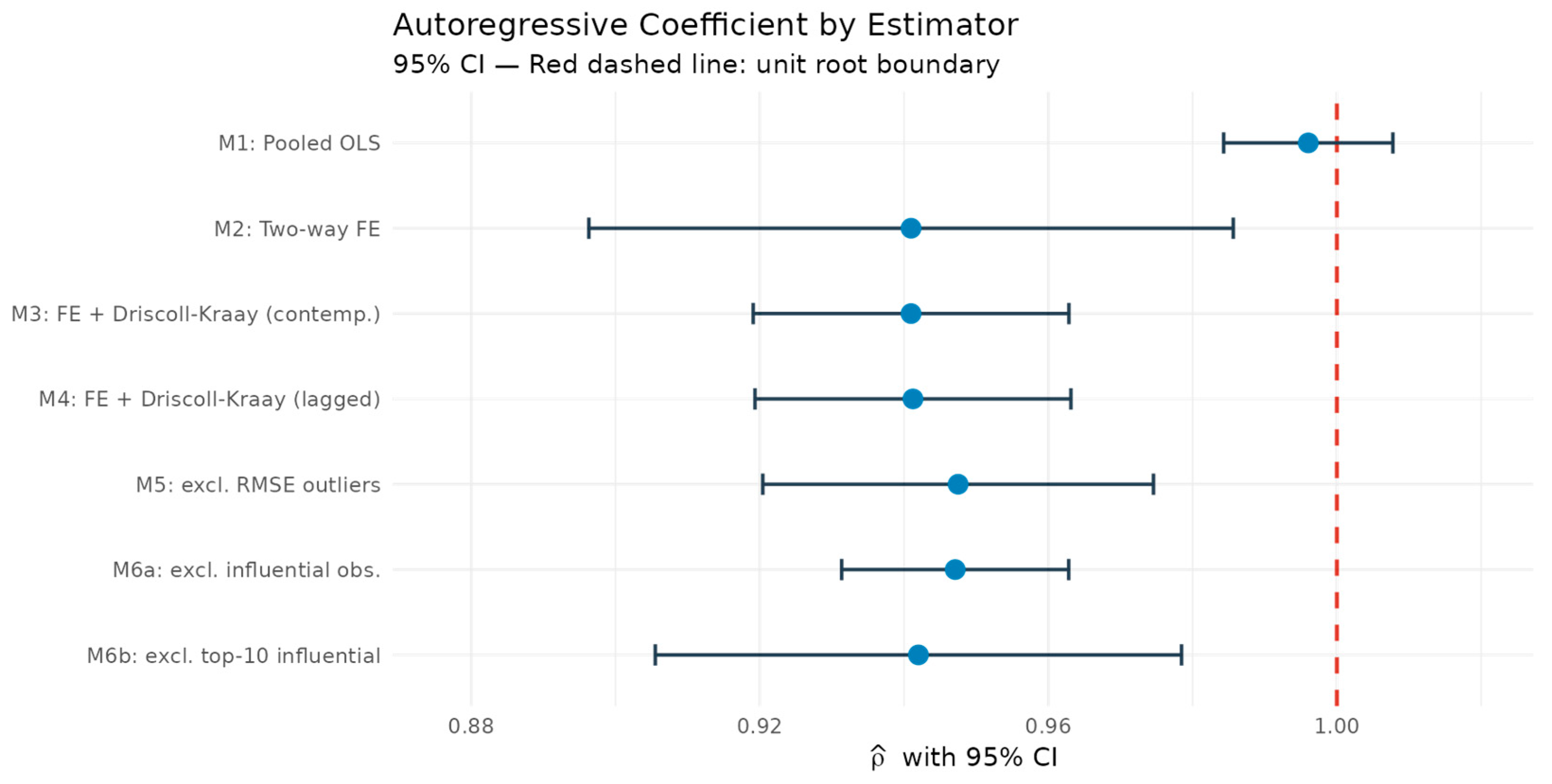
Estimates of food insecurity persistence are remarkably stable across estimators, as

Table 4. Autoregressive coefficient across estimators. 78 countries, 2010–2024.

Model	$\mathit{\rho }$	SE	95% CI	p-Value	Half-Life (yr)	DK Correction
M1: OLS Pooled	0.996	0.006	[0.984, 1.008]	<0.001	—	No
M2: FE Two-way	0.941	0.023	[0.896, 0.986]	<0.001	11.4	No
M3: FE + DK, contemp.	0.941	0.011	[0.919, 0.963]	<0.001	11.4	Yes
M4: FE + DK, lagged GGGI (t − 1)	0.941	0.011	[0.919, 0.963]	<0.001	11.4	Yes
M5: FE + DK, lagged, excl. RMSE outliers	0.947	0.014	[0.920, 0.975]	<0.001	12.9	Yes
M6a: FE + DK, lagged, excl. influential obs.	0.947	0.008	[0.931, 0.963]	<0.001	12.7	Yes
M6b: FE + DK, lagged, excl. top-10 influential	0.942	0.019	[0.906, 0.978]	<0.001	11.6	Yes

Source: authors’ own elaboration based on FAOSTAT (FIES severe food insecurity prevalence) and Global Green Growth Institute data. The bold row corresponds to the main specification. Half-life = ln(0.5)/ln($\rho$), computed only when the 95% CI excludes unity. DK = Driscoll-Kraay robust errors (maxlag = 4). The half-panel jackknife bias-corrected estimate for M4 is $\rho = 0.970$ (half-life of 22.9 years), so within-estimator half-lives are lower bounds.

shows. OLS pooled estimation (M1) yields $\rho = 0.996$ (SE = 0.006), an upper bound whose confidence interval includes unity: pooled estimation confounds true persistence with unobserved country heterogeneity, pushing the coefficient toward a unit root. The two-way FE estimator (M2) removes that heterogeneity and recovers $\rho = 0.941$ (SE = 0.023). The gap between M1 and M2 is the signature of heterogeneity bias, while the downward Nickell [7] bias of the within estimator is quantified below through a bias-corrected estimate.

M3 applies the Driscoll-Kraay correction to the same contemporaneous specification. The point estimate is unchanged ($\rho = 0.941$) and the standard error falls to 0.011, so the coefficient is estimated with high precision under the covariance structure that the diagnostics of Section 4.3 indicate.

The main specification is M4. With GGGI dimensions lagged one period, $\rho = 0.941$ (SE = 0.011, 95% CI [0.919, 0.963]), essentially identical to M2 and M3: the timing of the GGGI regressors leaves the persistence estimate unchanged, which indicates that the autoregressive component is not an artifact of regressor specification. The implied half-life is 11.4 years, and the confidence interval excludes both zero and unity. Because the within estimator understates $\rho$ in short panels, we also compute a half-panel jackknife bias-corrected estimate following Dhaene and Jochmans [28], which yields $\rho = 0.970$ and a half-life of roughly 23 years; the 11.4-year figure should therefore be read as a lower bound. The robustness variants M5, M6a, and M6b, detailed in Section 5.5, place $\rho$ between 0.942 and 0.947. Figure 1 displays all seven estimates graphically.

The dashed red line marks the unit root boundary ($\rho =1.0$). The M1 interval includes unity, reflecting a heterogeneity bias; the fixed-effects estimates cluster tightly between 0.941 and 0.947 (Table 4).

5.2. Contemporaneous Effects of GGGI Dimensions (M3)

Under the contemporaneous specification, once persistence is absorbed by the lagged dependent variable, only NCP reaches statistical significance, with a positive coefficient of 0.012 (SE = 0.005, p = 0.010); GEO is negative and marginal (−0.013, SE = 0.007, p = 0.066), while SI and ESRU are not significant. Contemporaneous associations between green growth dimensions and severe food insecurity are therefore weak, which is consistent with the transmission lags described in Section 3.2 and motivates the lagged specifications that Section 5.3 examines.

5.3. Lagged Effects: Temporal Profile of Green Growth Policies

Table 5. Temporal profile of GGGI effects on severe food insecurity. Two-way FE + Driscoll-Kraay (maxlag = 4). Dependent variable: AB2t. Lag structures are estimated independently.

Variable	t − 1 $\mathit{\beta }$	t − 1 SE	t − 2 $\mathit{\beta }$	t − 2 SE	t − 3 $\mathit{\beta }$	t − 3 SE
AB2t − 1	0.941 ***	0.011	0.932 ***	0.009	0.925 ***	0.010
SI_lagk	0.013	0.012	0.019	0.014	0.024	0.017
NCP_lagk	0.016 ***	0.004	0.010 *	0.004	0.008	0.008
GEO_lagk	−0.015	0.010	−0.013 *	0.006	−0.018 ***	0.005
ESRU_lagk	−0.023	0.023	−0.027 a	0.015	−0.034 **	0.011

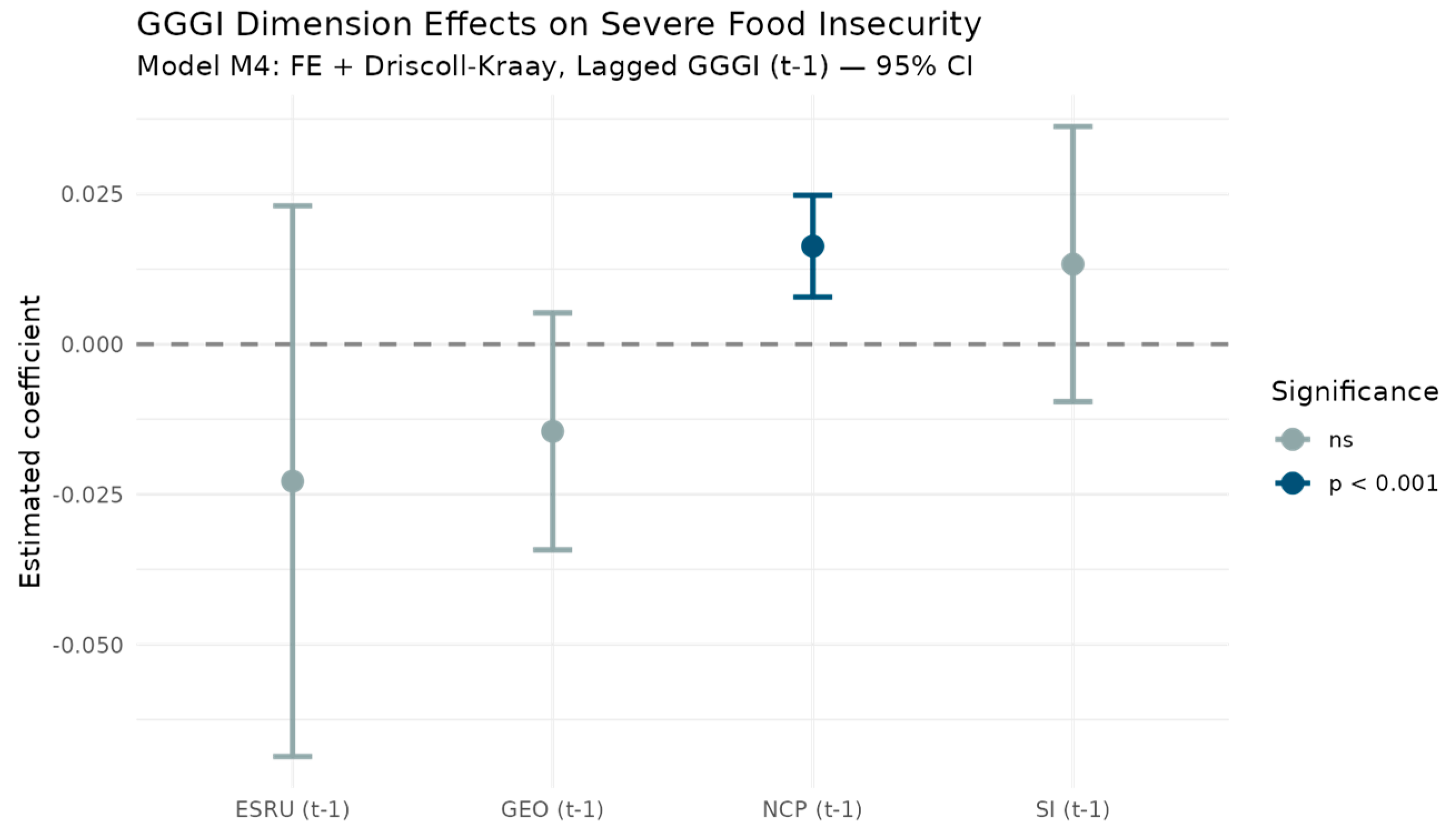
*** p < 0.001, ** p < 0.01, * p < 0.05, a p < 0.10. The lag profile shows that resource-use and green-opportunity associations materialize at longer horizons (t − 3), while natural capital protection displays a short-run association; Section 6.1 discusses the mechanisms underlying this temporal progression.

reports the GGGI dimension coefficients across three lag horizons. At $t-1$, only NCP is statistically significant, with a positive coefficient of 0.016 (SE = 0.004, p < 0.001). Countries that increased NCP scores in year $t-1$ experienced higher severe food insecurity in year t. GEO, SI, and ESRU at $t - 1$ are not significant (Figure 2). Section 5.5 examines the sensitivity of the NCP coefficient to influential units and to macroeconomic controls.

By $t-2$, the pattern begins to shift. GEO turns significant and negative: −0.013 (SE = 0.006, p = 0.033). NCP remains positive and significant (0.010, SE = 0.004, p = 0.019), while ESRU approaches significance (−0.027, SE = 0.015, p = 0.084). SI remains non-significant. At $t-3$, two dimensions show precisely estimated beneficial effects. GEO strengthens to −0.018 (SE = 0.005, p < 0.001) and ESRU becomes significant at −0.034 (SE = 0.011, p = 0.002). NCP loses significance entirely (0.008, SE = 0.008, p = 0.349). SI shows no significant coefficient at $t-1$, $t-2$, or $t-3$.

5.4. Heterogeneity by Income Level

Formal inference on heterogeneity rests on the fully interacted model described in Section 4.7, reported in

Table 6. Income-level heterogeneity: fully interacted model. Two-way FE + Driscoll-Kraay (maxlag = 4). Dependent variable: AB2t. Reference category: low-income countries.

Coefficient	Estimate	SE	Coefficient	Estimate	SE
AB2t − 1	0.951 ***	0.014	NCP_lag1 × High	−0.011	0.020
SI_lag1 (low income)	−0.122 *	0.052	NCP_lag1 × Lower-middle	0.058 ***	0.016
NCP_lag1 (low income)	−0.017	0.012	NCP_lag1 × Upper-middle	0.019	0.020
GEO_lag1 (low income)	−0.002	0.050	GEO_lag1 × High	−0.008	0.072
ESRU_lag1 (low income)	0.042	0.038	GEO_lag1 × Lower-middle	−0.006	0.056
SI_lag1 × High	0.147 *	0.062	GEO_lag1 × Upper-middle	−0.020	0.053
SI_lag1 × Lower-middle	0.165 **	0.063	ESRU_lag1 × High	−0.055	0.048
SI_lag1 × Upper-middle	0.145 **	0.051	ESRU_lag1 × Lower-middle	−0.044	0.037
			ESRU_lag1 × Upper-middle	−0.004	0.050

*** p < 0.001, ** p < 0.01, * p < 0.05. Joint Wald tests of homogeneity: SI ${\chi }^2\left(3\right) = 9.11$ (p = 0.028); NCP ${\chi }^2\left(3\right) = 18.97$ (p < 0.001); GEO ${\chi }^2\left(3\right) = 1.28$ (p = 0.735); ESRU ${\chi }^2\left(3\right) = 35.66$ (p < 0.001).

. The joint Wald tests reject effect homogeneity for three of the four dimensions: Social Inclusion (${\chi }^2\left(3\right) = 9.11$, p = 0.028), Natural Capital Protection (${\chi }^2\left(3\right) = 18.97$, p < 0.001), and ESRU (${\chi }^2\left(3\right) = 35.66$, p < 0.001); for GEO, homogeneity is not rejected (${\chi }^2\left(3\right) = 1.28$, p = 0.735).

The interaction structure is informative about where each association operates. For Social Inclusion, the coefficient for the low-income reference group is negative and significant (−0.122, SE = 0.052, p = 0.019), while the interaction terms for the three remaining income groups are positive, of almost exactly offsetting magnitude (0.145 to 0.165), and individually significant: the protective association of social inclusion is confined to low-income countries and averages out to zero in the pooled sample. For NCP, the adverse short-run association is concentrated in lower-middle-income countries (interaction 0.058, SE = 0.016, p < 0.001). For ESRU, heterogeneity is significant jointly although no individual contrast is precisely estimated, so we do not interpret specific pairwise differences.

The descriptive subsample estimates in

Table 7. Subgroup analysis: GGGI lagged effects by income level. Two-way FE + Driscoll-Kraay (maxlag = 3). Dependent variable: AB2t.

Coefficient	Low Income (n = 13)	Lower-Middle (n = 35)	Upper-Middle (n = 24)	High Income (n = 6)
$\rho$	0.904 ***	0.984 ***	0.900 ***	0.933 ***
SI_lag1	−0.124 a	0.034 a	0.020 a	0.025
NCP_lag1	0.044	0.030 ***	0.000	−0.028 *
GEO_lag1	−0.031	0.005	−0.032 ***	−0.014
ESRU_lag1	0.039	−0.012	0.032	−0.025

*** p < 0.001, * p < 0.05, a p < 0.10.

are consistent with the interaction results and show that no single GGGI dimension dominates across development stages. In low-income countries, Social Inclusion is the only dimension approaching significance, with a coefficient of $-$0.124 (p = 0.076); the remaining three dimensions fall well short of conventional thresholds. The lower-middle-income subsample tells a different story: NCP is positive and significant at 0.030 (SE = 0.009, p < 0.001), and it is this group that drives the pooled NCP result. Among upper-middle-income economies, GEO emerges as the dominant dimension, with a coefficient of $-$0.032 (SE = 0.006, p < 0.001) that actually exceeds the pooled estimate in absolute terms, suggesting that absorptive capacity moderates how effectively clean energy investment translates into food security gains. In high-income countries, NCP at $t-1$ is the only significant coefficient, estimated at $-$0.028 (SE = 0.014, p = 0.049), and notably its sign is negative, the reverse of what lower-middle-income economies show. Given that only six high-income countries are included, this subsample estimate is descriptive; formal inference rests on Table 6.

5.5. Robustness

The main findings hold under an expanded set of robustness checks, summarized in

Table 8. Robustness of Model M4 across Samples and Specifications. Two-way FE + Driscoll-Kraay (maxlag = 4). Dependent variable: AB2t. Coefficients with standard errors in parentheses.

Variable	M4	M5 Excl. RMSE	M6a Excl. obs.	M6b Excl. Top-10	Excl. 2020–2021	+log GDPpc	+log GDPpc, Infl.
AB2t − 1	0.941 *** (0.011)	0.947 *** (0.014)	0.947 *** (0.008)	0.942 *** (0.019)	0.953 *** (0.012)	0.935 *** (0.013)	0.939 *** (0.013)
SI_lag1	0.013 (0.012)	0.020 ** (0.007)	0.011 (0.007)	0.017 *** (0.005)	0.013 (0.016)	0.011 (0.012)	0.007 (0.013)
NCP_lag1	0.016 *** (0.004)	0.005 (0.006)	0.005 (0.004)	−0.010 (0.007)	0.008 *** (0.002)	0.017 *** (0.005)	0.015 ** (0.006)
GEO_lag1	−0.015 (0.010)	−0.010 (0.008)	−0.008 (0.008)	−0.002 (0.008)	−0.007 (0.007)	−0.015 (0.010)	−0.015 (0.010)
ESRU_lag1	−0.023 (0.023)	−0.002 (0.019)	−0.008 (0.014)	−0.008 (0.013)	−0.016 (0.025)	−0.033 (0.026)	−0.029 (0.027)
log GDPpc	—	—	—	—	—	−0.358 (0.372)	−0.516 (0.416)
Inflation (CPI)	—	—	—	—	—	—	−0.004 * (0.002)

*** p < 0.001, ** p < 0.01, * p < 0.05. M5 excludes Uganda, Mozambique, Rwanda, and Kenya (RMSE criterion); M6a excludes the 57 observations with Cook’s D > 4/n; M6b excludes the ten countries with the highest maximum Cook’s distance. Controls from World Bank WDI.

. Varying the Driscoll-Kraay bandwidth across maxlag = 2, 3, and 5 shifts point estimates by no more than 0.002 in any specification. Excluding the four RMSE outlier countries (M5), all 57 influential observations (M6a), or the ten most influential countries (M6b) leaves the autoregressive coefficient between 0.942 and 0.947; excluding the pandemic years 2020 and 2021 yields $\rho$ = 0.953, and the specifications augmented with log GDP per capita and CPI inflation yield 0.935 and 0.939. Persistence is therefore invariant to influential units, crisis periods, and macroeconomic controls.

The GGGI coefficients respond to sample composition in an informative way. The NCP association at t − 1 survives the exclusion of the pandemic years (0.008, p < 0.001) and both control specifications (0.017, p < 0.001; 0.015, p = 0.007), but attenuates when the high food insecurity countries identified by the influence diagnostics are excluded, while the SI coefficient turns positive and significant in those same subsamples (M5: 0.020, p = 0.002; M6b: 0.017, p < 0.001). This pattern is what the interaction model of Section 5.4 predicts: the identifying variation for the low-income SI association and for the lower-middle-income NCP association is concentrated precisely in the high-prevalence countries, so removing them shifts the pooled coefficients toward the values of the remaining income groups. We read the attenuation as composition, not fragility, and Section 6.3 develops this point.

6. Discussion of the Results Obtained

6.1. The Temporal Mismatch

What emerges from the analysis is that green growth progress is associated with food security outcomes, but on a timeline that differs from what most evaluations assume. GEO and ESRU show no statistically detectable effects at one year. By the second year, GEO turns negative and significant; by the third, both dimensions do. The pattern is consistent with the gestation periods described in Section 3.2.

In economic terms, the associations at $t-3$ imply that a ten-point improvement in ESRU, roughly one standard deviation, is associated with about 0.34 percentage points lower severe food insecurity prevalence, and the equivalent figure for GEO is about 0.18 points; against a sample mean of 12.4 percent, these are modest single-year magnitudes, which is precisely why the persistence result dominates the policy reading.

On the other hand, He et al. [2] report positive effects of using System GMM over a fifteen-year panel of Sub-Saharan African countries. Ajeigbe and Ganda [4], working with contemporaneous specifications across a broader sample, find mixed or null results. Studies with longer panels capture the delayed effects that contemporaneous designs miss; the disagreement traces back to where each study sits on the transmission timeline.

Finally, NCP behaves differently, and we read its pattern as a sequencing problem rather than a permanent trade-off. The coefficient is positive and significant at one and two years, then becomes indistinguishable from zero by year three. Hickel and Kallis [18] raise the possibility that green growth contains inherent contradictions. The data point to a more specific mechanism: policies that restrict land use can reduce agricultural access for smallholders and disrupt local food supply chains before ecosystem service benefits (pollination, water regulation, and soil stabilization) begin to offset those losses.

6.2. Persistence as Structural Constraint

The autoregressive coefficient of 0.941 implies a half-life of 11.4 years, and the half-panel jackknife correction indicates that even this figure understates the inertia: the bias-corrected estimate of 0.970 corresponds to a half-life of roughly 23 years. A country at the 75th percentile of the food insecurity distribution would need, absent structural intervention, well over a decade to halve the gap to the cross-country mean. Against that inertia, the strongest estimated GGGI association at three years is ESRU at −0.034 per index point. The mixed unit root evidence of Section 4.3, with first-generation tests rejecting a unit root and CIPS failing to reject it, reinforces this reading: severe food insecurity behaves as a near-integrated process in which shocks and policy gains alike dissipate very slowly. This is the econometric signature of a structural trap.

6.3. Income Heterogeneity and Absorptive Capacity

The interaction model confirms formally that the operative GGGI dimension depends on development stage: joint Wald tests reject homogeneity for Social Inclusion, Natural Capital Protection, and ESRU. In low-income countries, Social Inclusion is protective, and the offsetting interaction terms for the remaining income groups explain why its pooled coefficient is indistinguishable from zero: the prediction that social inclusion transmits fastest through household consumption (H3) is supported precisely where that channel binds.

When poverty is extreme, direct transfers, school meals, and health access move outcomes faster than green technology or resource efficiency, which remain downstream problems requiring infrastructure that may not yet exist. Lower-middle-income countries drive the pooled NCP result. Conservation policy, without complementary support, appears to increase food insecurity in the short run. Upper-middle-income economies show the opposite pattern. GEO is negative and significant, and its coefficient exceeds the pooled estimate, suggesting that absorptive capacity allows clean energy investment and green technology adoption to translate into productivity gains within a year. Among high-income countries, only NCP turns negative, inverting the sign found in lower-middle-income economies. Only six countries, so caution is warranted; but the sign flip points toward a level-of-development moderator for the NCP-food security relationship that Li et al. [12] and Sun et al. [29] document in other regional contexts. Green growth effectiveness is conditional on the institutional and economic infrastructure that determines whether policy translates into outcomes at all.

6.4. Limitations

Five limitations deserve explicit statement. (1) Identification. Lagged GGGI predictors improve on contemporaneous specifications but do not provide exogenous instruments. If a country experiences a multi-year shock (conflict, drought, terms-of-trade collapse) that simultaneously depresses both food security and green investment, the lagged values remain correlated with the error; as Angrist and Pischke [30] emphasize, lag structure alone does not guarantee strict exogeneity, and the estimates reported here are conditional dynamic associations rather than treatment effects. (2) Remaining unobserved confounders. Two-way fixed effects absorb time-invariant heterogeneity and common shocks, and the control specifications of Section 5.5 address income and price dynamics, but country-specific climate shocks and conflict exposure on two- to three-year cycles could bias coefficients toward zero; the associations at three years are best read as lower bounds. (3) Near-integration of the dependent variable. With the CIPS test unable to reject a unit root, statistics that depend on $1/(1-\rho )$, such as long-run multipliers, are unreliable, which is why the analysis reports impact associations and treats half-lives as lower bounds. (4) Measurement floor. FAO reports severe food insecurity prevalence with limited variation at very low levels, so several high-income series are nearly constant; this compresses within-country variation precisely where prevalence is lowest and is one reason inference for the high-income group rests on the interaction model. (5) Composite indices and sample coverage. GGGI dimensions are composites: two countries can score identically on GEO through very different policy mixes with different transmission times, and the balanced panel excludes countries with weaker statistical systems, so external validity is strongest for economies resembling those included. The observation window also includes the 2011 food price spike, the 2015–2016 El Niño, COVID-19, and the 2022 price crisis; year fixed effects absorb common components, but country-specific responses could contaminate the estimates, as Perego et al. [31] document for Central America.

7. Conclusions

Two questions structured this paper: how persistent is severe food insecurity, and over what horizon is green growth progress associated with it? On the first, severe food insecurity behaves as a near-integrated process. The autoregressive coefficient of 0.941 is a lower bound; the bias-corrected estimate reaches 0.970, and shocks dissipate over decades rather than years. Second, the associations are real but delayed and income-conditional: Green Economic Opportunities emerge at two years and strengthen at three, Efficient and Sustainable Resource Use at three, and Natural Capital Protection displays a short-run adverse association, concentrated in lower-middle-income countries, that dissipates by the third year. Social Inclusion is protective only in low-income countries, where the consumption channel binds.

Two implications follow for policy. Development agencies and national governments that assess green growth programs against annual outcome metrics will systematically understate their returns; GEO- and ESRU-oriented investment requires evaluation windows of at least three years. And because the operative dimension depends on income level, portfolio composition should differ by development stage: social inclusion instruments where structural poverty binds, green economic opportunities where productive capacity can absorb clean technology, and complementary support wherever conservation policy temporarily constrains smallholder production.

Three directions for future work follow. Identification rests on predetermined GGGI values; plausibly exogenous variation, such as international climate finance commitments that differentially affect GGGI investment by dimension, could move from conditional associations toward causal estimates. Nonlinear or threshold specifications conditional on institutional quality would extend the linear framework. Finally, the transition cost associated with Natural Capital Protection is an average across lower-middle-income contexts; program-level analysis of specific conservation interventions (national park expansions, protected area designations, wetland restoration) would allow direct testing of the mechanism.

References

1. FAO; IFAD; UNICEF; WFP; WHO. The State of Food Security and Nutrition in the World 2025; FAO: Rome, Italy, 2025. [Google Scholar] [CrossRef]
2. He, J.; Osabohien, R.; Yin, W.; Adeleke, O.K.; Uduma, K.; Agene, D.; Su, F. Green economic growth, renewable energy and food security in Sub-Saharan Africa. Energy Strategy Rev. 2024, 55, 101503. [Google Scholar] [CrossRef]
3. Osabohien, R.; Karakara, A.A.; Ashraf, J.; Matthew, O.; Osabuohien, E.; Onolade, O.; Waheed, N. Green economy and food security in Africa. Environ. Dev. Sustain. 2025, 27, 28873–28889. [Google Scholar] [CrossRef]
4. Ajeigbe, K.B.; Ganda, F. Leveraging food security and environmental sustainability in achieving sustainable development goals: Evidence from a global perspective. Sustainability 2024, 16, 7969. [Google Scholar] [CrossRef]
5. Aali-Bujari, A.; Jiménez-Preciado, A.L.; Venegas-Martínez, F. Effects of CO2, N2O, CH4 emissions and adjusted net national income on food security in 86 countries. Int. J. Energy Econ. Policy 2026, 16, 1003–1019. [Google Scholar] [CrossRef]
6. Aguilar-Rivera, N. Sustainable biofuels. Strategy for growth and energy security. Rev. Mex. Econ. Finanz. 2022, 17, e498. [Google Scholar] [CrossRef]
7. Nickell, S. Biases in dynamic models with fixed effects. Econometrica 1981, 49, 1417–1426. [Google Scholar] [CrossRef]
8. Driscoll, J.C.; Kraay, A.C. Consistent covariance matrix estimation with spatially dependent panel data. Rev. Econ. Stat. 1998, 80, 549–560. [Google Scholar] [CrossRef]
9. FAO. Measuring Hunger, Food Security and Food Consumption. Access to Food. Available online: https://www.fao.org/measuring-hunger/access-to-food/en (accessed on 31 January 2026).
10. Mohamed, G.; Chiad, F.; Abdesslam, M.; Omar, B.; AL-Absy, M.S.M. Identifying determinants of food security using panel data analysis: Evidence from Maghreb countries. Economies 2024, 12, 91. [Google Scholar] [CrossRef]
11. Cruz-Sánchez, Y.; Aguilar-Estrada, A.; Baca-del Moral, J.; Monterroso-Rivas, A.I. The availability of food in Mexico: An approach to measuring food security. Agric. Food Secur. 2024, 13, 35. [Google Scholar] [CrossRef]
12. Li, M.; Zhang, Y.; Fan, Z.; Chen, H. Evaluation and research on the level of inclusive green growth in Asia-Pacific region. Sustainability 2021, 13, 7482. [Google Scholar] [CrossRef]
13. Chang, T.; Gupta, R.; Inglesi-Lotz, R.; Simo-Kengne, B.; Smithers, D.; Trembling, A. Renewable energy and growth: Evidence from heterogeneous panel of G7 countries using Granger causality. Renew. Sustain. Energy Rev. 2015, 52, 1405–1412. [Google Scholar] [CrossRef]
14. Ceesay, E.K.; Ndiaye, M.B.O. Climate change, food security and economic growth nexus in the Gambia: Evidence from an econometrics analysis. Res. Glob. 2022, 5, 100089. [Google Scholar] [CrossRef]
15. Hoechle, D. Robust standard errors for panel regressions with cross-sectional dependence. Stata J. 2007, 7, 281–312. [Google Scholar] [CrossRef]
16. Pal, S.; Lean, H.H.; Villanthenkodath, M.A. Achieving sustainable food security: Integrating environmental and governance issues. J. Environ. Stud. Sci. 2026, 16, 283–297. [Google Scholar] [CrossRef]
17. Bodirsky, B.L.; Beier, F.; Humpenöder, F.; Leip, D.; Crawford, M.S.; Chen, D.M.-C.; von Jeetze, P.; Springmann, M.; Soergel, B.; Nicholls, Z.; et al. A food system transformation pathway reconciles 1.5 °C global warming with improved health, environment and social inclusion. Nat. Food 2025, 6, 1133–1152. [Google Scholar] [CrossRef] [PubMed]
18. Hickel, J.; Kallis, G. Is green growth possible? New Polit. Econ. 2020, 25, 469–486. [Google Scholar] [CrossRef]
19. Osabohien, R.; Karakara, A.A.; Ashraf, J.; Al-Faryan, M.A.S. Green environment–social protection interaction and food security in Africa. Environ. Manag. 2023, 71, 835–846. [Google Scholar] [CrossRef] [PubMed]
20. Global Green Growth Institute. Global Green Growth Index Dataset; Global Green Growth Institute: Seoul, Republic of Korea, 2024; Available online: https://gggi.org/global-green-growth-index/ (accessed on 31 January 2026).
21. Wooldridge, J.M. Econometric Analysis of Cross Section and Panel Data; MIT Press: Cambridge, MA, USA, 2002. [Google Scholar]
22. Pesaran, M.H. General Diagnostic Tests for Cross Section Dependence in Panels; CESifo Working Paper No. 1229; Social Science Research Network: Rochester, NY, USA, 2004. [Google Scholar] [CrossRef]
23. Im, K.S.; Pesaran, M.H.; Shin, Y. Testing for unit roots in heterogeneous panels. J. Econom. 2003, 115, 53–74. [Google Scholar] [CrossRef]
24. Maddala, G.S.; Wu, S. A comparative study of unit root tests with panel data and a new simple test. Oxf. Bull. Econ. Stat. 1999, 61, 631–652. [Google Scholar] [CrossRef]
25. Hadri, K. Testing for stationarity in heterogeneous panel data. Econom. J. 2000, 3, 148–161. [Google Scholar] [CrossRef]
26. Pesaran, M.H. A simple panel unit root test in the presence of cross-section dependence. J. Appl. Econom. 2007, 22, 265–312. [Google Scholar] [CrossRef]
27. Elliott, G.; Rothenberg, T.J.; Stock, J.H. Efficient tests for an autoregressive unit root. Econometrica 1996, 64, 813–836. [Google Scholar] [CrossRef]
28. Dhaene, G.; Jochmans, K. Split-panel jackknife estimation of fixed-effect models. Rev. Econ. Stud. 2015, 82, 991–1030. [Google Scholar] [CrossRef]
29. Sun, Y.; Ding, W.; Yang, Z.; Yang, G.; Du, J. Measuring China’s regional inclusive green growth. Sci. Total Environ. 2020, 713, 136367. [Google Scholar] [CrossRef] [PubMed]
30. Angrist, J.D.; Pischke, J.S. Mostly Harmless Econometrics: An Empiricist’s Companion; Princeton University Press: Princeton, NJ, USA, 2009. [Google Scholar]
31. Perego, V.M.E.; Brown, M.; Ceballos, F.; Hernández, M.; Berrospi, M.L.; Pereira, L.D.; Salcedo, S.; Benjamin, M.P.; Flores, L.; Mora, E. Precios Internacionales y Seguridad Alimentaria: Un Análisis de la Transmisión de los Precios de los Alimentos y Fertilizantes en América Central; World Bank: Washington, DC, USA, 2024. [Google Scholar]
Figure 1. Autoregressive coefficient by estimator (95% CI).
Sustainability 18 07557 g001
Figure 2. GGGI dimension coefficients, Model M4: FE + Driscoll-Kraay, Lagged t 1 (95% CI). Dark blue point = significant at p < 0.001. Gray points = not significant. NCP ( t 1 ) is the only dimension with a statistically precise estimate at this lag. Source: authors’ own elaboration based on FAOSTAT and Global Green Growth Institute data.
Sustainability 18 07557 g002