Industrial Structure Optimization for Improving Multidimensional Land Use Performance: A Spatial Empirical Study of Zhejiang Province, China

Abstract

Land and industrial systems form the cornerstone of regional sustainable development. Widespread misuse of land often accompanies industrial structure evolution (ISE), making the promotion of comprehensive land use benefits (LUB) a pivotal obstacle to regional sustainability. This study establishes an integrated framework to evaluate the dynamic characteristics of ISE and its interactive responses to multidimensional (ecological, social, and economic) LUB. The ISE assessment covers long-term changes in industrial investment, employment, and economic output, while LUB systematically integrates the ecological, social, and economic values of land resources. Combined with an enhanced genetic algorithm, a multi-objective optimization model is constructed and applied to 33 counties in Zhejiang Province, China. The results indicate that regional LUB exhibits obvious spatial heterogeneity and staged evolution from 2000 to 2020, with the regional industrial structure transforming from industrial-driven to service-oriented. The proposed model formulates targeted industrial adjustment pathways to resolve tertiary industry overinvestment and unbalanced secondary industry development. The optimization effectively promotes comprehensive land use sustainability, realizing differentiated regional progress including economic upgrading in the east, multidimensional coordination in the south, social benefit improvement in the north, and ecological sustainability promotion in the west. This study provides theoretical and practical references for high-quality regional sustainable development.

1. Introduction

Land and industry are the bedrock of regional development. However, the traditional growth model, characterized by extensive factor inputs, is increasingly unsustainable due to its high resource consumption and environmental pressures. Imbalanced industrial structures trigger unregulated expansion of industrial layouts and land use, which creates compound developmental conflicts covering resources, ecology and society. Uncontrolled non-agricultural construction occupies vast woodland, high-quality cultivated land and ecological corridors. This permanently fragments habitat connectivity and degrades the integrity of natural ecosystems, leading to irreversible losses of critical ecosystem services including carbon sequestration and oxygen release, soil and water conservation, biodiversity conservation, and food provision. Meanwhile, blind expansion of low-end service industries and structural distortions in secondary industries generate extensive, low-efficiency land use practices. Such practices intensify resource depletion and exacerbate surface runoff, soil erosion and water exploitation pressure, forming a vicious cycle. Misallocated production factors drive unplanned land sprawl; in turn, continuous degradation of ecosystem services restricts the coordinated and sustainable improvement of economic and social benefits from land use.

This limitation underscores the imperative for structural transformation and efficiency enhancement to foster a more resilient and advanced economic structure. New Structural Economics posits that economic growth is fundamentally structure-driven, with the optimization and upgrading of industrial structure serving as key engines for sustained regional socioeconomic development [1]. China currently navigates a critical juncture of new urbanization and economic paradigm shifts that is marked by tightening resource constraints and evolving growth dynamics, which presents both a vital window for industrial restructuring and an opportunity to effectively surmount growth bottlenecks, fundamentally alter development paradigms, and steadfastly elevate quality of life. However, persistent issues of “pseudo-advancement” and “insufficient rationalization” within China’s industrial structure lead to challenges like inefficient land use and declining social and ecological benefits [2]. Consequently, optimizing industrial structure allocation and comprehensively enhancing land use benefits are not only practical necessities for regional land management but also pivotal pathways for transitioning from scale-driven expansion to quality-oriented growth. Building on this foundation, the present study investigates land use benefits through the lens of industrial structure optimization, considering internal investment, employment, and output. We develop a multi-objective optimization model employing an enhanced genetic algorithm to integrate economic, social, and ecological benefit dimensions, thus moving beyond the limitations of previous single-objective studies. Focusing on county-level units, this research developed tailored industrial structure adaptation strategies by analyzing the disparities between the optimal and actual proportions of various industrial factors. This analysis helped identify the potential for boosting economic, social, and ecological benefits in different counties.

Research on the evolution of industrial structure can be traced back to the 17th century. Scholars first observed, from a macro perspective, the phenomenon of labor shifting from agriculture to industry and commerce in pursuit of higher returns, gradually establishing the three-sector model and laying the empirical foundation for evolutionary theory [3,4,5]. In the field of industrial structure evaluation, international research has established assessment methodologies, such as the Shift-Share Analysis (SSM) proposed by Kuznets [6], as well as subsequent derivatives including the structural deviation and competitive deviation components [7]. Subsequent studies have placed greater emphasis on the diversity of evaluation subjects and the systematicity of dimensions. The scope of research not only encompasses macro-level overall structures but also extends to specific industrial types, integrating multiple perspectives such as sustainable development theory, input–output models, and spatial correlation analysis for empirical investigation [8,9,10]. These efforts have significantly enhanced the applicability and scientific rigor of the evaluation system. Regarding influencing factors, earlier international studies have focused on macro-level elements such as resource allocation, consumer demand, and technological innovation [11,12]. In contrast, domestic research has placed greater emphasis on empirical analysis. For example, Li et al. [13] observed that the information services industry exhibits an indirect relationship with the secondary industry, while its connections with the tertiary industry are primarily economic. Gou [14] found that urbanization and investment in science and technology promote industrial transformation, whereas foreign investment exhibits an inhibitory effect. Kang et al. [15] demonstrated that extensive growth and fiscal imbalances exacerbate structural distortions, while financial development and social investment can mitigate such distortions. The research spans multiple scales, from national to provincial and municipal levels, reflecting the increasing depth of domestic studies in integrating theoretical and empirical approaches, as well as bridging macro- and micro-level perspectives.

In the field of land use benefit, international studies on economic benefits began relatively early. Baffour Awuah et al. [16] highlighted that scientific planning can significantly enhance the economic benefits of land use, while Deines et al. [17] cautioned against overlooking land suitability, which may lead to an overestimation of returns. Domestic research, although initiated relatively later, has developed rapidly and encompasses multiple spatial scales. For instance, Yang et al. [18] employed a coupling coordination model to analyze the spatial differentiation of economic benefits in Zhejiang Province; Cai [19] examined the economic mechanisms of rural land use from the perspective of rural tourism; and He [20] validated a positive correlation between urban scale and economic benefits. In the realm of social benefit research, a unified framework has not yet converged internationally, while domestic studies remain in an exploratory phase. For example, Chen et al. [21] established an evaluation system based on equity and livelihood; Liu et al. [22] compared the net social benefits of different land use types; and Zhou et al. [23] applied TOPSIS and gray models to evaluate and predict social benefits. In terms of ecological benefits, international research early focused on the concept and assessment of ecosystem service value. For instance, Daily [24] and Costanza et al. [25] systematically defined and classified this theory, while Brauman et al. [26] simulated ecological benefits under different scenarios using dynamic models. Domestic studies have been extensively conducted at various scales such as watersheds, provinces, and cities [27,28,29]. The research methods primarily fall into two categories: one involves constructing indicator systems using AHP, the entropy method, or comprehensive evaluation approaches [30,31], while the other employs quantitative assessments through models such as ecological footprint and green equivalent. The research scope has also expanded to include perspectives like carbon storage and ecological conservation redlines [32,33], significantly enhancing the systematic nature and practicality of ecological benefit research.

Scholarly inquiry into the relationship between industrial structure and land use benefit generally proceeds from three theoretical perspectives. Firstly, the industrial determinism perspective posits that regional industrial structure and its developmental level constrain the allocation and efficiency of land resources. Industrial structures formed at different stages of economic development exhibit significant variations in land use demands, with diverse and complex response mechanisms [34,35]. Some studies indicate that industrial structure change is the decisive factor in land use pattern shifts, though the magnitude of change in the two may not necessarily be synchronous [36]. Other scholars contend that the direction and timing of change in both are fundamentally consistent, with only the rate differing [37]. Furthermore, research moving beyond the “dual-structure” framework has approached the issue from an industrial planning perspective, proposing that industrial development should guide land strategies and resource allocation [38].

A second perspective, termed land determinism, asserts that the rational configuration of land use forms the indispensable foundation and prerequisite for industrial upgrading and broader socioeconomic development. Under this framework, land use structure not only provides the material underpinning for industrial growth but also functions as a crucial impetus for structural adjustment [39,40]. Utilizing econometric modeling, Zhang et al. [41] empirically demonstrated that the alignment of land use structures with economic systems is conducive to enhanced land use benefits and the successful realization of macro-policy objectives. Further empirical investigations reveal that distinct variations in land use structure exert differential influences on the pattern, trajectory, and pace of regional economic development [42].

A third perspective from coordination theory emphasizes creating synergy between industrial structure and land use. It contends that such coupling is essential for enhancing land use benefits and industrial optimization. Land serves as a spatial foundation for industries, supporting their development through its productive, living, and ecological functions. Conversely, industrial allocation realizes land value, while industrial activities shape land use patterns and benefits [43]. Empirical evidence confirms this reciprocity. Meng [44] found industrial restructuring intensified land use in Beijing, with land policies guiding industrial transformation. Ma [45] examined urban industrial–land coupling, highlighting coordinated strategies to boost benefits and reduce land consumption. Similarly, Fan [46] advocated scientific planning of industrial types and layouts to promote regional coordination through suitability evaluation.

Although extensive research has been devoted to the relationship and causal identification between industrial structure and land use benefits, the dynamic interactions between the two, as well as systematic approaches to diagnosing industrial structural imbalances and identifying potential for improving land use benefits, remain understudied. Furthermore, the input–output models commonly used in existing research are suitable for rapid economically oriented assessments at a macro scale and mainly describe sectoral interdependence. This paper centers on the allocation optimization of nine internal industrial factors, making the two lines of research complementary to each other. County-level regions, serving as fundamental units for industrial transformation and land resource allocation, often represent weak links in regional coordinated development. They commonly face challenges such as insufficient industrial efficiency and low land use productivity.

Based on this, the study analyses how the optimization of industrial structure affects the multidimensional benefits of land use and how this relationship can be optimized at the district level. It should be clarified that this study focuses on one of the core dimensions of sustainability, namely economic sustainability. Specifically, it explores the impact pathways of multidimensional industrial features (internal investment structure, employment allocation and output efficiency) on land use benefits from the perspective of industrial restructuring. This research develops an improved genetic algorithm optimization model to coordinate economic, social and ecological benefits, which addresses the limitations of conventional single-objective models. Taking counties as basic research units, this paper proposes targeted regulation strategies for industrial structure adjustment, quantifies the room for growth of each county in terms of economic, social and ecological benefits, and supports regional sustainable development during economic transition.

2. Materials and Methods

2.1. Case Study

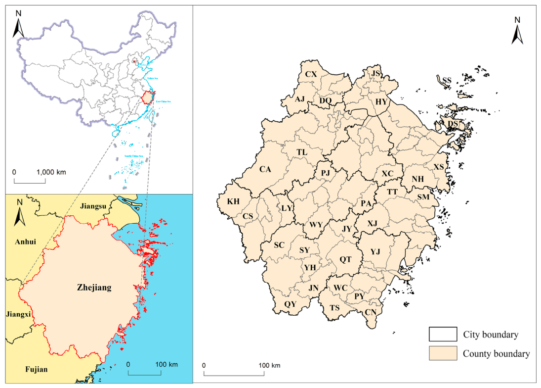
Situated along China’s southeastern coast, Zhejiang Province (118°01′–123°10′ E, 27°06′–31°11′ N) is a pivotal economic, cultural and transportation hub comprising 11 major cities. In 2021, it represented 4.1% of China’s population and generated a substantial regional GDP of 6.5 trillion yuan, a testament to its national economic importance [47]. However, administrative reorganizations frequently introduce inconsistencies into regional data. Therefore, to facilitate a robust analysis of regional development challenges, this study concentrates on 33 historically stable and traditional counties, which provide a more dependable basis for investigation (

Table 1. List of narrowly defined counties in Zhejiang Province.

Region	Prefecture-Level City	County (Abbreviation)
Eastern Coastal	Ningbo	XS, NH
	Shaoxing	XS
	Zhoushan	DS, SS
Southern Coastal	Wenzhou	YJ, PY, CN, WC, TS
	Taizhou	SM, TT, XJ
Central-Western	Jinhua	WY, PJ, PA
	Quzhou	CS, KH, LY
Southwestern	Lishui	QT, JY, SC, SY, YH, QY, JN
Northern	Hangzhou	TL, CA
	Jiaxing	JS, HY
	Huzhou	DQ, CX, AJ

and Figure 1). To improve recognition in images, the names of counties have been abbreviated.

Table 2. The corresponding abbreviations for the 33 sampled counties.

Counties	Abbreviations	Counties	Abbreviations	Counties	Abbreviations
Xiangshan	XS	Ninghai	NH	Xinchang	XC
Daishan	DS	Shengsi	SS	Yongjia	YJ
Pingyang	PY	Cangnan	CN	Wencheng	WC
Taishun	TS	Sanmen	SM	Tiantai	TT
Xianju	XJ	Wuyi	WY	Pujiang	PJ
Panan	PA	Changshan	CS	Kaihua	KH
Longyou	LY	Qingtian	QT	Jinyun	JY
Suichang	SC	Songyang	SY	Yunhe	YH
Qingyuan	QY	Jingning	JN	Tonglu	TL
Chunan	CA	Jiashan	JS	Haiyan	HY
Deqing	DQ	Changxing	CX	Anji	AJ

shows the corresponding abbreviations for each county.

2.2. Data Acquisition

Data on industrial development and socioeconomic indicators were primarily obtained from the China Statistical Yearbook, the Zhejiang Statistical Yearbook, and statistical yearbooks and government statistical bulletins of various cities, counties, and districts from 2000 to 2020. Data on land use status and ecological environment indicators were mainly sourced from the Institute of Geographic Sciences and Natural Resources Research, Chinese Academy of Sciences, the China Land and Resources Statistical Yearbook, the China Environmental Statistical Yearbook, and the Zhejiang Provincial Ecological and Environmental Status Bulletin. Missing values were supplemented using linear interpolation.

3. Methodology

3.1. Establishing Evaluation System

3.1.1. Comprehensive Evaluation System for LUB

Land use benefit (LUB) studies exhibit indicator bias, following either a two-dimensional input–output framework [48] or an economic–social–ecological framework [49]. Based on existing studies and this research’s theoretical framework, a three-dimensional indicator system was constructed for evaluating LUB, as detailed in

Table 3. Evaluation index system of LUB.

Target Layer	Criteria Layer	Index Layer	Unit	Direction	Weight
LUB	Social benefit	Population density	capita/km2	−	0.0065
		Annual disposable income of urban residents	104 Yuan/capita	+	0.0268
		Urban built-up area per capita	m2/capita	+	0.0207
		Road areas per capita	m2/capita	+	0.0273
		Number of hospital beds per ten thousand persons	Bed/104 people	+	0.0197
		Total retail sales of consumer goods per unit land area	104 Yuan/km2	+	0.0694
		Number of employed persons at year-end per unit land area	capita/km2	+	0.0380
	Ecological benefit	Grassland coverage rate	%	+	0.0064
		Park green space area per 10,000 persons	Km2/104 persons	+	0.0245
		Intensity of industrial smoke and dust emission	t/km2	−	0.0026
		Intensity of industrial SO2 emission	t/km2	−	0.0026
		Nitrogen oxides emissions per unit land area	t/km2	−	0.0024
		(Comprehensive Surface) Runoff Coefficient	Dimensionless	−	0.0054
		Impervious Surface Coverage Rate	%	−	0.0041
		Water Resources Exploitation and Utilization Intensity	%	−	0.0028
	Economic benefit	GDP per unit land area	104 Yuan/km2	+	0.0730
		Fiscal revenue per unit land area	104 Yuan/km2	+	0.0809
		Year-end deposit balance of financial institutions per unit land area	104 Yuan/km2	+	0.0755
		Actual use of foreign capital per unit land area	104 Yuan/km2	+	0.0895
		Intensity of investment in fixed assets	104 Yuan/km2	+	0.1564
		Intensity of gross output of primary industry	104 Yuan/km2	+	0.1156
		Intensity of gross output of secondary industry	104 Yuan/km2	+	0.0730
		Intensity of gross output of tertiary industry	104 Yuan/km2	+	0.0770

.

3.1.2. Comprehensive Assessment System for ISE

During urban development, industrial structure is reflected in its corresponding investment, employment, and output structures. These represent the allocation of production factors across development stages, with different combinations exhibiting distinct characteristics [50,51]. Accordingly, this study constructs an industrial structure evolution (ISE) assessment system based on these three dimensions (

Table 4. Assessment index system of ISE.

Target Level	Criteria Layer	Index Layer	Unit	Direction	Weight
ISE	Employment structure	Percentage of employment in primary industry	%	+	0.11915
		Percentage of employment in secondary industry	%	+	0.03429
		Percentage of employment in tertiary industry	%	+	0.03048
	Investment structure	Percentage of investment in primary industry	%	+	0.40036
		Percentage of investment in secondary industry	%	+	0.07486
		Percentage of investment in tertiary industry	%	+	0.08994
	Output structure	Percentage of output value of primary industry	%	+	0.13813
		Percentage of output value of secondary industry	%	+	0.05048
		Percentage of output value of tertiary industry	%	+	0.06232

).

3.1.3. Data Processing

We adopted the entropy method for objective weighting to avoid the potential biases of subjective approaches. This method is particularly suited for our study, as it retains original indicator information, is less sensitive to data distribution, and handles large-scale indicator systems effectively—matching our data characteristics and evaluation needs. Addressing this, we first standardized all indicators, including the multidimensional LUB indicator, to eliminate any potential bias in weight assignment arising from differences in units, currencies, or volatility. This ensures the reliability of the entropy-based weights. The detailed calculation steps are as follows:

$$X=\left[\begin{array}{lll}{x}_{1,1}\hfill & \dots \hfill & x_{1,j}\hfill \\ ⋮\hfill & \ddots \hfill & ⋮\hfill \\ x_{1,j}\hfill & \dots \hfill & x_{i,j}\hfill \end{array}\right]$$

(1)

$$V_{ij}={\displaystyle \frac{x_{ij}-x_{\min }}{x_{\max }-x_{\min }}}$$

(2)

$$p_{ij}={\displaystyle \frac{V_{ij}}{{\displaystyle {\sum }_{i=1}^n{V}_{ij}}}}$$

(3)

$$\begin{array}{l}{E}_j=-{\displaystyle \frac{1}{\ln n}}{\displaystyle \sum _{i=1}^n{p}_{ij}}\times \ln p_{ij}\\ (i=1,2,3,\dots n;j=1,2,3,\dots ,m)\end{array}$$

(4)

$$g_j=1-E_j(j=1,2,3,\dots ,m)$$

(5)

$${\omega }_j={\displaystyle \frac{g_j}{{\displaystyle {\sum }_{j=1}^m{g}_j}}}(j=1,2,3,\dots ,m)$$

(6)

$$W={({\omega }_1,{\omega }_2,\dots ,{\omega }_m)}^T$$

(7)

Equations (1) and (2) mean the data normalization, Equation (3) represents the index normalization, Equation (4) describes the entropy value calculation of each indicator, and Equations (5)–(7) correspond to the weight calculation. x represents the indicator matrix for the 33 counties in Zhejiang, v_ij denotes the normalized result of the j-th indicator for the i-th county, x_ij denotes the original value of the j-th indicator for the i-th county, x_max represents the maximum original value of the indicator across all regions, x_min represents the minimum original value of the indicator. p_ij represents the probability of the j-th indicator for the i-th county, E_j represents the information entropy value for the j-th indicator, g_j represents the information utility value for the j-th indicator, ω_j stands for the weight of the indicator, and W is the objective weight vector for all indicators.

After determining the weights of each indicator, the LUB index and ISE index for each county were computed using a weighted method.

$$E_t={\displaystyle \sum _{j=1}^m{\omega }_j\times V_{ij}}(t=L,I)$$

(8)

EL and EI represent the level of LUB and ISE, respectively.

3.2. Multi-Objective Optimization Model

3.2.1. Multi-Objective Optimization Strategy

Based on the previous theoretical analysis of the correlation mechanism between ISE and LUB above, this study employs Spearman correlation analysis to reveal the characteristics of the relationship between ISE and LUB across 33 counties over a twenty-year period, as shown in

Table 5. Spearman’s correlation coefficient (ρ) and statistical significance (P) between ISE and LUB.

	Economic Benefit (a)	Social Benefit (b)	Ecological Benefit (c)
Industrial structure evolution (ISE)	−0.66 (0.000 ***)	−0.61 (0.000 ***)	−0.39 (0.000 ***)

Note: Absolute value of ρ: 0.00–0.19 indicates extremely weak or no correlation; 0.20–0.39 denotes weak correlation; 0.40–0.69 signifies moderate correlation; ≥0.70 represents strong correlation. ***, **, and * denote significance levels of 1%, 5%, and 10%, respectively.

.

As shown in Table 5, the ISE level of the 33 counties exhibits a moderate negative correlation with economic and social benefit levels and a weak negative correlation with ecological benefit levels. All correlation coefficients are statistically significant at the 1% level. The results demonstrate a significant statistical association between the two variables, suggesting a probable nonlinear relationship.

Spatial heterogeneity exists across counties in terms of industrial development stages, resource endowments and land use development patterns. Global correlation analysis can only reflect the overall statistical correlation between variables and fails to characterize the nonlinear evolutionary characteristics within individual counties. Therefore, a county-level polynomial regression model was adopted in this study [52,53]. For each of the 33 counties and each of the three benefit variables (economic, social, and ecological), we constructed first-, second-, and third-order polynomial models. The models were systematically compared using adjusted R², AIC, and BIC as the core metrics. The significance of the coefficient of the highest-order term (p < 0.1) was also used as a constraint to exclude higher-order models that might otherwise be selected solely because of improved goodness of fit despite an insignificant highest-order term. Among the candidate models satisfying the significance constraint, the model order with the lowest BIC was selected as the final order. Compared with AIC, BIC imposes a stronger penalty on the number of parameters and is therefore more suitable for the small-sample setting of this study, thereby effectively curbing overfitting. The specific model specifications are presented as follows:

$$\begin{array}{l}{a}_i=k_{a_0,i}+k_{a_1,i}{s}_i+\dots +k_{a_n,i}{s}_i^n\\ b_i=k_{b_0,i}+k_{b_1,i}{s}_i+\dots +k_{b_n,i}{s}_i^n\\ c_i=k_{c_0,i}+k_{c_1,i}{s}_i+\dots +k_{c_n,i}{s}_i^n(n=1,2,3;i=1,2,\dots 33)\end{array}$$

(9)

In Equation (9) above, a_i, b_i, and c_i represent the economic, social, and ecological benefit levels of the i-th county, respectively; k_an,i, k_bn,i, and k_cn,i, indicate the coefficients of economic, social, and ecological benefits for the i-th county, respectively; n represents the polynomial degree; and s_i denotes the ISE level of the i-th county:

$$s_i=x_{1,i}+x_{2,i}+x_{3,i}+x_{4,i}+x_{5,i}+x_{6,i}+x_{7,i}+x_{8,i}+x_{9,i}$$

(10)

where x_1,i, x_2,i, and x_3,i denote the share levels of the primary, secondary, and tertiary industries in the output structure of the i-th county, respectively. x_4,i, x_5,i, and x_6,i represent the share levels of the primary, secondary, and tertiary industries in the employment structure of the i-th county, respectively. And x_7,i, x_8,i, and x_9,i indicate the share levels of the primary, secondary, and tertiary industries in the investment structure of the i-th county, respectively.

Our objective function aims to simultaneously maximize the levels of economic benefit (a_i), social benefit (b_i), and ecological benefit (c_i):

$$\max \left\{a_i+b_i+c_i\right\}$$

(11)

In the experimental section, key parameters are set as follows: the population size is 100, and the maximum number of generations is 2000. The algorithm demonstrates excellent performance in both convergence speed and solution accuracy. Detailed parameters are shown in Appendix A.

3.2.2. Variable Settings for the Model

The variables are denoted as x_1,i to x_9,i, where x_1,i, x_2,i, and x_3,i denote the share levels of the primary, secondary, and tertiary industries in the output structure of the i-th county, respectively. x_4,i, x_5,i, and x_6,i represent the share levels of the primary, secondary, and tertiary industries in the employment structure of the i-th county, respectively. And x_7,i, x_8,i, and x_9,i indicate the share levels of the primary, secondary, and tertiary industries in the investment structure of the i-th county, respectively.

3.2.3. Determination of Constraints and Optimization Strategies

$$\begin{array}{l}{x}_{1,i}/{\omega }_{1,i}+x_{2,i}/{\omega }_{2,i}+x_{3,i}/{\omega }_{3,i}=1\\ x_{4,i}/{\omega }_{4,i}+x_{5,i}/{\omega }_{5,i}+x_{6,i}/{\omega }_{6,i}=1\\ x_{7,i}/{\omega }_{7,i}+x_{8,i}/{\omega }_{8,i}+x_{9,i}/{\omega }_{9,i}=1\end{array}$$

(12)

ω_i stands for the weight of the indicator. At different stages of urban development, the industrial structure corresponds to specific investment, employment, and output-value structures. This essentially reflects variations in the types and quantities of production factors invested during different developmental periods, and different combinations of these factors will exhibit distinct characteristics in the evolution of the industrial structure. However, no matter how the combination changes, the sum of the proportions of the three different industrial types always equals 1 (100%).

To establish reasonable constraints for industrial structure adjustment, this study first established an empirical basis using historical data, noting that the average variation range of industrial structure across the 33 counties during the study period was between −26.03% and 24.59%. To further calibrate the thresholds, we selected county samples representing high-, medium-, and low-level development and systematically evaluated the optimization benefits under six different constraint ranges, from ±5% to ±30%. The results indicate that a ±20% constraint not only ensures significant optimization effects but also aligns with the transition cost theory emphasized by Wang et al. [54] and the practical industrial transformation goals of the counties, thereby ensuring strategic relevance and practical feasibility of the planning scheme. Consequently, this study ultimately adopted the constraint that the change in the proportion of each industrial sector relative to the base year (2020) should not exceed ±20%. Under this constraint, the optimal decision-making solution was determined by maximizing the sum of a_i, b_i, and c_i.

3.3. Response Model

To quantitatively characterize the interactive relationship between land use benefit and industrial structure evolution, this study introduces the concept of “response intensity”. This concept aims to measure the sensitivity and feedback magnitude of changes in one aspect to changes in the other. Specifically, the evolution of the industrial structure drives changes in land use benefit, while changes in land use benefit can be viewed as a response to the influence of industrial structure evolution. To quantitatively assess the degree and characteristics of this response, drawing on relevant research [51], a response intensity model of land use benefit to industrial structure evolution was developed. This model consists of two core components: a response index model and a response intensity model.

$$\eta =\left(d{E}_L/d{E}_I\right)\times \left(E_L/E_I\right)$$

(13)

$$\mu =\left|\eta \right|$$

(14)

η denotes the response index of urban land use efficiency to industrial structure evolution; EL and EI represent the level of land use benefit (LUB) and industrial structure evolution (ISE), respectively, where d_EL/d_EI represents the derivative of industrial structure evolution with respect to urban land use benefit. µ indicates the responsiveness of urban land use efficiency to industrial structure changes. A higher value of µ suggests a stronger response of land use benefit to industrial structure evolution, and conversely, a lower value implies a weaker response. Both η and µ are dimensionless.

3.4. Spatial Autocorrelation Analysis

This study quantitatively analyzes the spatial clustering of comprehensive benefits at the county level. We construct a K-nearest neighbor spatial weight matrix and conduct spatial statistical tests with Global Moran’s I and Local Indicators of Spatial Association (LISA). We also test different neighborhood parameters to verify the robustness of our findings. Certain counties in the research area are geographically isolated without shared boundaries with adjacent units. To address this problem, we use a symmetric 4-nearest neighbor weight matrix and standardize its rows. Statistical significance is assessed via 9999 permutation tests (p < 0.05). Global Moran’s I quantifies the overall degree of spatial clustering across the entire study region, while Moran scatter plots visually display local spatial correlations. LISA classifies local spatial units into four cluster categories: high-high, low-low, high-low and low-high. These quantitative outputs serve as solid evidence for interpreting spatial patterns and establish a full analytical workflow.

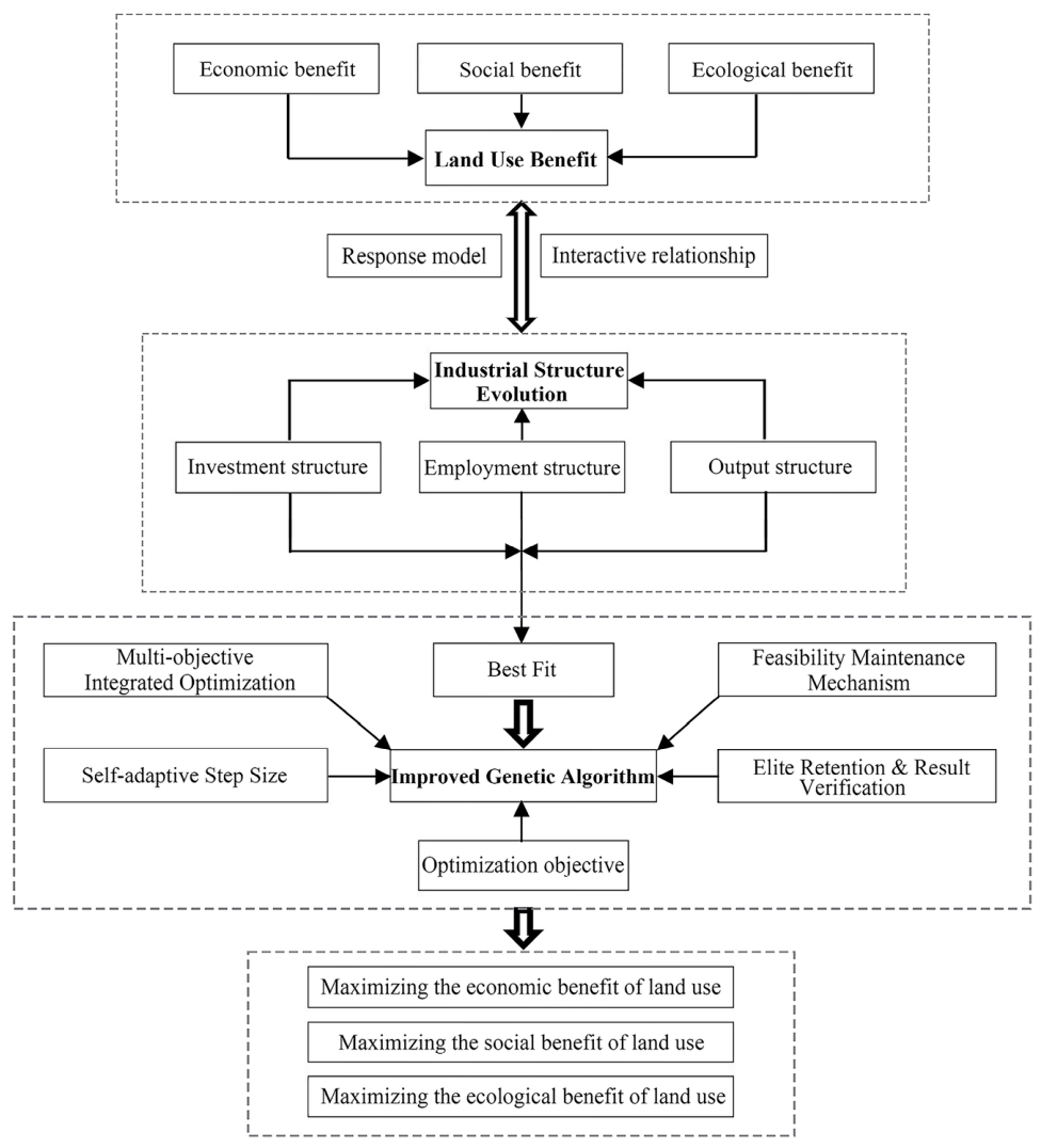
Based on the research methodologies outlined in Section 3.1, Section 3.2, Section 3.3 and Section 3.4 above, the overall research framework constructed in this study is illustrated in Figure 2.

4. Results

4.1. Global and Local Spatiotemporal Autocorrelation of Economic, Social and Ecological Benefits

4.1.1. Temporal Evolution of Global Spatial Autocorrelation

Table 6. Global Moran’s I for economic, social, and ecological benefits, 2000–2020.

Year	Economic Benefits	Social Benefits	Ecological Benefits
2000	0.533 ***	0.441 ***	−0.094 ns
2005	0.563 ***	0.643 ***	0.144 *
2008	0.560 ***	0.611 ***	0.308 **
2010	0.582 ***	0.649 ***	0.336 ***
2015	0.618 ***	0.575 ***	0.330 ***
2018	0.608 ***	0.495 ***	0.369 ***
2020	0.623 ***	0.529 ***	0.417 ***

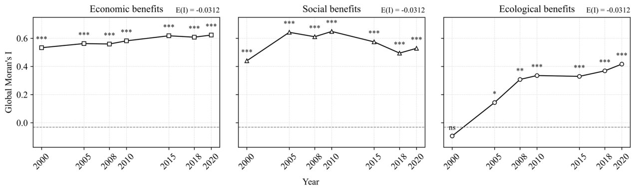
Note: *, **, and *** denote permutation-test significance at p < 0.05, p < 0.01, and p < 0.001, respectively; ns denotes non-significance. The expected value under spatial randomness is E(I) = −0.03125.

and Figure 3 illustrate the Global Moran’s I values and their temporal variations in county-level economic, social and ecological benefits across the study period. Economic benefits exhibited strong and consistently significant positive spatial autocorrelation throughout the study period. Global Moran’s I increased from 0.533 in 2000 to 0.623 in 2020, with only minor short-term fluctuations between 2005 and 2008 and between 2015 and 2018. The overall increase indicates a gradual strengthening of spatial sorting: counties with relatively high economic benefits became increasingly surrounded by other high-value counties, whereas low-value counties tended to remain adjacent to similarly low-value neighbors. The persistence of Moran’s I above 0.53 in every year demonstrates that the economic pattern was not a temporary configuration but a stable regional structure.

Social benefits also displayed pronounced positive spatial dependence, although their temporal trajectory was less monotonic. Moran’s I rose sharply from 0.441 in 2000 to 0.643 in 2005, reached its maximum of 0.649 in 2010, and subsequently declined to 0.495 in 2018 before recovering modestly to 0.529 in 2020. Thus, the spatial concentration of social benefits was strongest during approximately 2005–2010 and weakened thereafter, while remaining highly significant in all years. This pattern suggests that the spatial organization of social benefits was more temporally responsive than that of economic benefits but still retained a clear regional clustering structure.

Ecological benefits followed a fundamentally different trajectory. In 2000, Moran’s I was negative and statistically non-significant (I = −0.094, p = 0.242), indicating that the county-level distribution did not depart systematically from spatial randomness. A weak but significant positive association emerged in 2005 (I = 0.144, p = 0.044), after which the index increased to 0.308 in 2008, 0.336 in 2010, and 0.417 in 2020. The transition from a non-significant pattern to moderate positive autocorrelation indicates the progressive formation and consolidation of ecological benefit clusters. In other words, ecological differentiation became increasingly spatially organized over time rather than remaining a set of isolated county-level variations.

4.1.2. Moran Scatter Plots and the Structure of Local Spatial Association

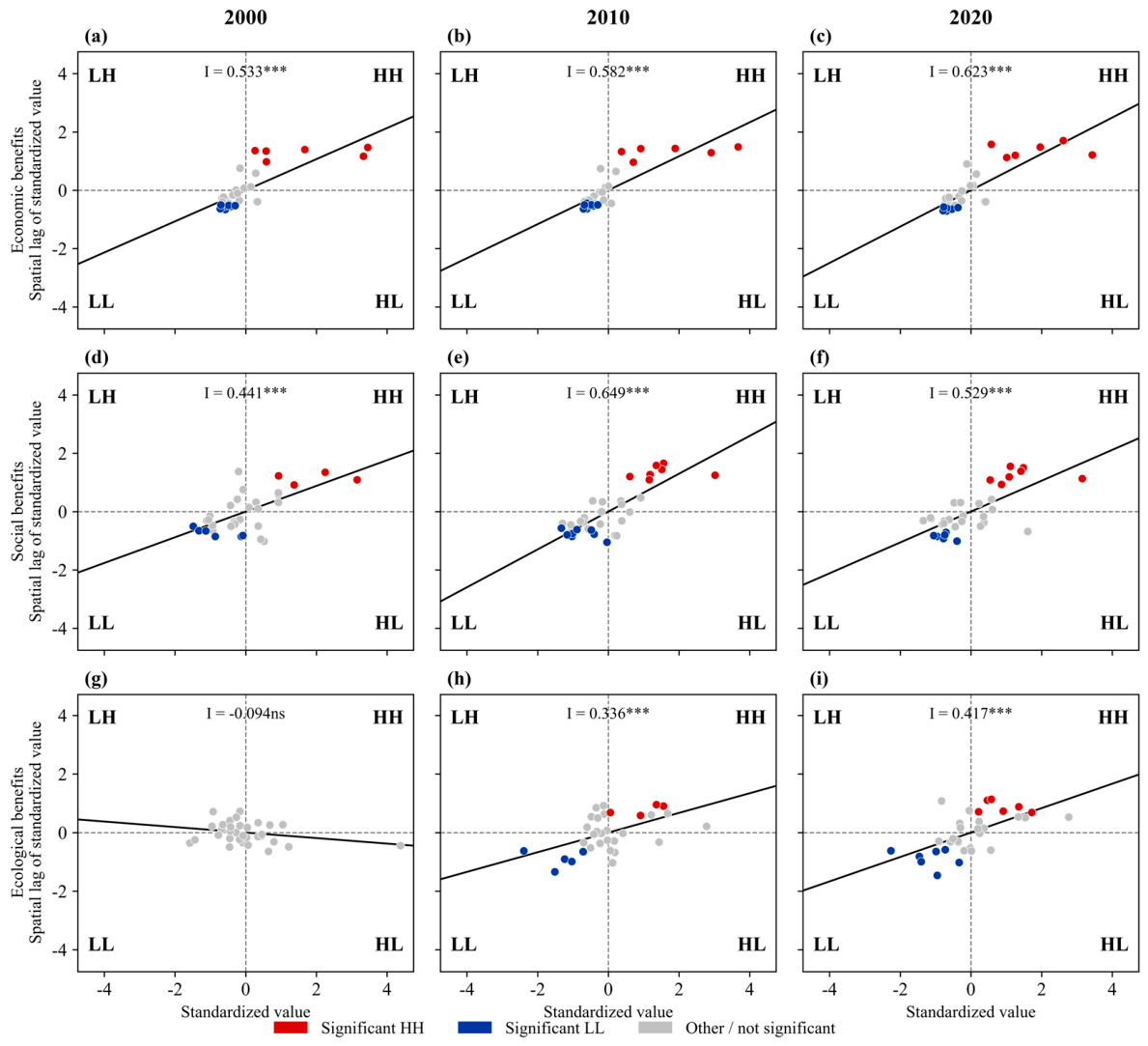
The Moran scatter plots corroborate the global statistics while revealing the composition of the spatial association (Figure 4). For economic benefits, the regression line is positive and becomes progressively steeper from 2000 to 2020. Significant observations are concentrated mainly in the high–high (HH) and low–low (LL) quadrants, whereas high–low (HL) outliers are virtually absent. This configuration indicates a relatively coherent core–periphery pattern in which high- and low-value counties form internally consistent regional regimes, with few counties displaying values that sharply contradict those of their neighbors.

The social benefit scatter plots similarly show positive spatial association, but they contain more local outliers in 2000 and 2010. These HL observations represent counties with relatively high social benefits embedded within lower-value neighborhoods and therefore identify transitional or locally exceptional units. By 2020, the disappearance of significant HL and LH outliers and the continued presence of HH and LL groups indicate a reduction in local discontinuities and a clearer separation between high-value and low-value spatial regimes. Nevertheless, the lower slope in 2020 relative to 2010 confirms that the overall strength of clustering weakened after its earlier peak.

The ecological benefit scatter plot for 2000 is nearly horizontal and dominated by non-significant observations around the origin, consistent with the absence of global spatial autocorrelation. By 2010 and 2020, observations extend more clearly into the HH and LL quadrants and the fitted slope becomes positive, demonstrating the emergence of spatially coherent ecological regimes. The simultaneous presence of HH, LL, HL, and LH counties also indicates that ecological benefits developed a more heterogeneous local structure than economic benefits, including both stable clusters and spatial transition zones.

4.1.3. Evolution of LISA Clusters

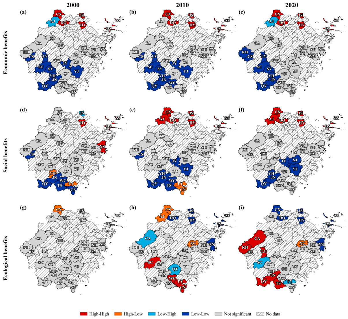
Figure 5 presents the LISA cluster maps reflecting county-level economic, social, and ecological benefits in 2000, 2010 and 2020;

Table 7. Overall LISA cluster composition in selected years (%).

Indicator	Year	HH	HL	LH	LL	NS
Economic benefits	2000	18.2	0.0	3.0	27.3	51.5
Economic benefits	2010	18.2	0.0	0.0	30.3	51.5
Economic benefits	2020	18.2	0.0	3.0	24.2	54.5
Social benefits	2000	12.1	6.1	3.0	18.2	60.6
Social benefits	2010	21.2	6.1	0.0	24.2	48.5
Social benefits	2020	21.2	0.0	0.0	18.2	60.6
Ecological benefits	2000	0.0	3.0	0.0	0.0	97.0
Ecological benefits	2010	12.1	9.1	6.1	18.2	54.5
Ecological benefits	2020	18.2	3.0	6.1	21.2	51.5

further quantifies the overall composition of LISA clusters in the selected years (unit: %).

The Economic benefit maps reveal the most stable spatial configuration among the three dimensions. The HH cluster remained anchored in the northern region—particularly JS, DQ, HY, and CX—and in the eastern island counties of DS and SS. These six counties accounted for 18.2% of the study units in each benchmark year, indicating a persistent high-value core rather than a temporary concentration. In contrast, LL clusters were concentrated in the southwestern and central-western regions. The southwestern LL share was 85.7% in both 2000 and 2010 and remained high at 71.4% in 2020, while the central-western LL share increased from 33.3% in 2000 and 2010 to 50.0% in 2020. This pattern quantitatively supports a broad high-value concentration in northern/eastern counties and a low-value concentration in western and southwestern counties.

The spatial organization of social benefits changed more substantially over time. In 2000, the eastern coastal region contained the principal HH concentration, with 60.0% of its counties classified as HH, whereas only 14.3% of northern counties belonged to this category. By 2010, the northern HH share had expanded to 71.4% and remained at this level in 2020, while the eastern coastal HH share stabilized at 40.0%. This shift indicates that the dominant high-social-benefit core consolidated in northern Zhejiang, particularly in JS, HY and AJ, while DS and SS formed a smaller eastern coastal HH cluster. Low-social-benefit clustering was concentrated mainly in the southwest and, to a lesser extent, the southern coastal region.

Ecological benefits exhibited the clearest spatial restructuring. In 2000, 97.0% of counties were not significant, and CX was the only significant spatial outlier. By 2010, a differentiated pattern had emerged: 37.5% of southern coastal counties were classified as HH, while 60.0% of eastern coastal counties and 42.9% of northern counties were classified as LL. The simultaneous occurrence of HH clusters in the south and LL clusters in the north and east represents a spatial configuration that contrasts sharply with the economic and social dimensions. By 2020, ecological HH clusters had expanded and become more geographically dispersed. They included 33.3% of central-western counties, 28.6% of southwestern counties, 12.5% of southern coastal counties, and 14.3% of northern counties. At the same time, LL clusters remained prominent in the eastern coastal region (60.0%) and strengthened in the north (57.1%). This redistribution indicates that ecological high-value areas increasingly emerged in inland and southwestern counties, whereas several northern and eastern counties formed persistent low-value ecological clusters.

4.2. Evolution Characteristics of ISE

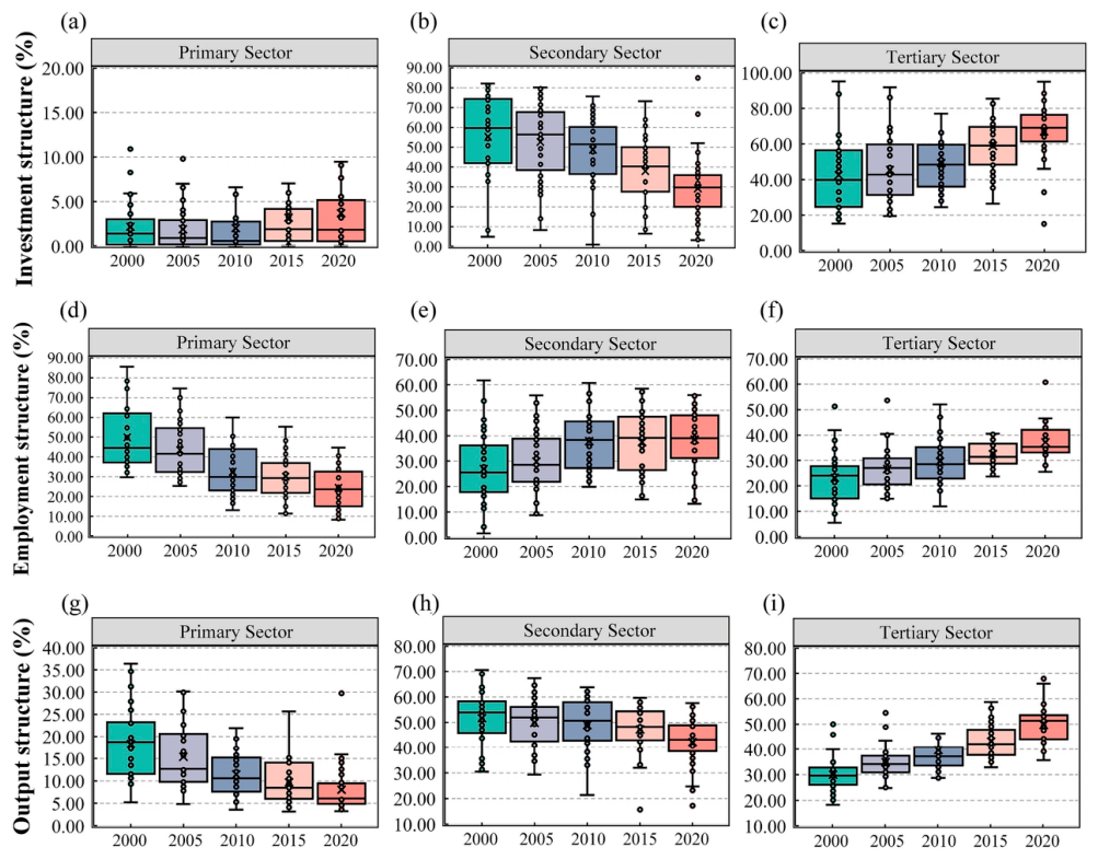
Figure 6a–c analyzes Zhejiang’s county-level investment structure (2000–2020). The primary sector remained marginal (<3% median), but its interquartile range (IQR) expanded post-2015, indicating growing disparities. The secondary sector declined steadily (median ~60% to ~30%), with a contracting IQR signaling industrial concentration. The tertiary sector became dominant (median ~40% to ~70%), and its tightening IQR after 2010 reveals strong convergence towards a service-based economy.

Figure 6d–f illustrates employment structure evolution. Primary-sector employment declined markedly (median ~40% to ~20%), with a narrowing IQR suggesting reduced inter-county disparities. The secondary sector expanded (median ~25% to ~40%), becoming dominant by 2020, though its wide IQR indicates persistent regional differences. The tertiary sector increased gradually (26% to ~35%), with a shortening IQR signifying more coordinated development.

Figure 6g–i shows output-value structure. The primary sector’s median share dropped sharply (~20% to ~5%). The secondary sector remained stable near 50% pre-2010, then gradually declined to ~45%, with enduring regional heterogeneity. The tertiary sector grew steadily (~30% to >50%), becoming the dominant contributor, with a shortening box length indicating spatial convergence. Overall, the primary sector diminished, the secondary sector declined with imbalances, and the tertiary sector emerged as the new, robust leading force.

4.3. Evolution Characteristics of Response Degree

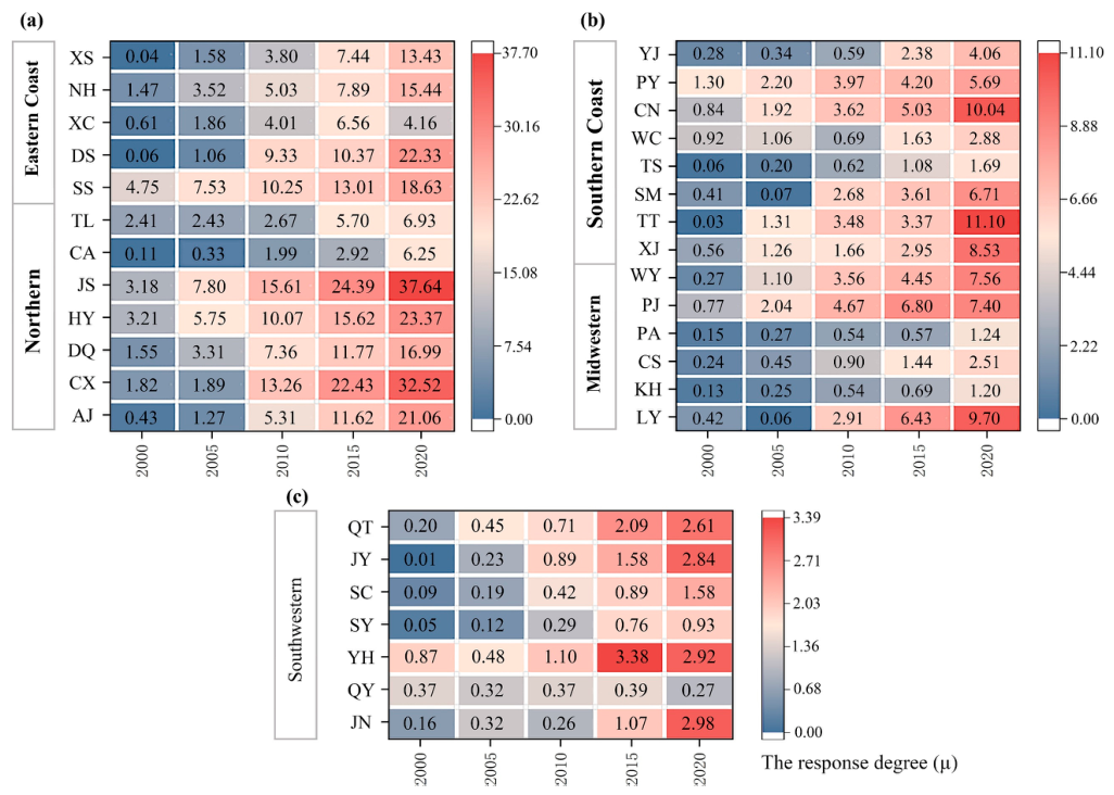
As shown in Figure 7, the responsiveness of land use benefits to industrial structure evolution in Zhejiang’s counties showed a consistent increasing trend over time, with notable spatiotemporal heterogeneity across development stages. The eastern coastal and northern regions exhibited significantly higher overall responsiveness, with initial values in 2000 ranging from 0.04 to 4.75. By 2020, these areas had formed a distinct high-responsiveness core zone. The southern coastal and central-western regions displayed a multipolar development pattern, reflecting the pronounced influence of industrial restructuring on land use efficiency. However, certain counties—including TS in the southern coastal area and PA and KH in the central-western region—still recorded low responsiveness levels (<1.69) as of 2020. The southwestern region lagged behind overall, with most areas remaining below 3.0. In general, the sensitivity of land use benefits to industrial transformation has risen markedly, particularly since 2010, highlighting its growing relevance as a critical dimension in regional development studies.

5. Discussion

5.1. Optimization Strategies for the Investment, Employment and Output Structure of Primary, Secondary, and Tertiary Industries

Table 8. Differences between optimized and actual shares of the primary, secondary and tertiary industries in terms of investment, employment and output structure.

Region		Investment Structure (%)			Employment Structure (%)			Output Structure (%)
		Primary	Secondary	Tertiary	Primary	Secondary	Tertiary	Primary	Secondary	Tertiary
Eastern Coastal	XS	−0.05	−1.95	−2.05	−1.40	−8.23	6.89	−2.50	8.66	−7.59
	NH	−0.21	−2.25	−8.34	−1.37	−8.63	8.02	−1.31	9.82	−8.72
	XC	1.57	−4.79	3.22	−0.10	3.00	−7.10	0.97	−9.91	9.01
	DS	0.00	3.01	−3.01	−3.44	−6.65	8.65	−3.10	9.69	−6.95
	SS	0.00	−1.19	−9.25	−4.92	−2.92	7.84	−5.95	3.39	2.57
Southern Coastal	YJ	1.53	−2.68	1.15	4.99	2.06	−7.08	0.61	−8.63	8.94
	PY	1.11	−3.31	2.20	4.57	2.02	−6.59	0.64	−8.97	9.05
	CN	0.24	−4.15	5.65	3.36	3.64	−7.00	0.86	−8.21	8.48
	WC	1.82	−1.25	−0.56	5.88	2.24	−8.12	1.21	−4.63	4.40
	TS	2.50	−0.66	−3.96	6.04	−1.20	−5.01	1.08	−6.71	7.29
	SM	−0.07	−9.40	6.56	−4.72	−1.02	5.69	−2.24	8.69	−7.85
	TT	−0.34	7.83	−9.62	−4.53	−5.56	8.62	−0.86	8.22	−9.18
	XJ	−0.03	6.36	−9.33	−5.91	−0.68	6.59	−1.12	8.75	−8.97
Central-Western	WY	−0.02	−4.65	−7.97	−2.64	3.28	−0.64	−1.18	9.86	−8.67
	PJ	−0.03	−2.21	−4.62	−2.40	−7.04	6.50	−0.83	8.28	−9.22
	PA	−0.16	4.07	−7.19	−5.16	−1.44	6.60	−1.68	7.64	−8.24
	CS	−0.93	6.94	−7.22	−2.76	−6.91	6.98	−0.92	8.38	−9.14
	KH	−0.46	5.14	−8.00	−8.23	1.79	6.43	−1.41	7.14	−8.33
	LY	−0.27	9.20	−8.37	−6.77	−0.14	6.92	−1.06	8.42	−9.01
Southwestern	QT	−0.20	6.32	−9.14	−6.22	−0.61	6.87	−0.69	8.59	−9.39
	JY	−0.11	4.91	−8.13	−7.38	1.71	5.65	−0.92	9.16	−9.18
	SC	−0.62	6.00	−8.51	−7.13	0.48	6.66	−1.56	7.78	−8.39
	SY	−0.30	6.41	−9.09	−8.35	2.72	5.61	−1.92	8.13	−8.10
	YH	2.88	−4.29	1.41	4.36	4.22	−8.58	1.17	−9.23	8.06
	QY	−1.90	3.72	−1.77	−8.94	1.87	7.07	−1.38	7.54	−8.49
	JN	−0.19	2.24	−4.51	−8.38	0.73	7.62	−1.02	4.94	−7.25
Northern	TL	0.41	−6.53	7.82	3.68	4.97	−8.64	1.17	−9.19	8.60
	CA	−0.35	0.64	−0.33	−8.10	−1.09	9.22	−1.99	6.13	−7.22
	JS	−0.02	2.16	−4.22	−1.33	−8.39	7.11	−0.74	9.45	−8.70
	HY	−0.38	−3.59	−5.20	−1.83	−7.88	7.06	−0.66	8.48	−7.82
	DQ	−0.31	−1.36	−9.75	−1.82	−8.18	7.99	−0.92	8.74	−7.82
	CX	−2.78	4.74	−8.84	−2.24	0.59	1.66	−1.11	9.89	−8.98
	AJ	0.00	6.96	−5.66	−1.99	−8.06	8.25	−1.09	9.02	−9.02

presents the differences between the optimized and current structures of the primary, secondary, and tertiary sectors in terms of investment, employment, and output across 33 counties in Zhejiang. Positive values indicate a deficit in factor inputs, while negative values indicate surplus factor inputs. In the investment dimension, the mismatch is most serious in the counties of central and western Zhejiang. These counties generally face insufficient investment in the secondary sector (with deviations of +9.20% for LY and +6.94% for CS) and excessive investment in the tertiary sector (with a deviation of −9.14% for QT). Across the province, the absolute deviation in primary-sector investment is below 2.88% in every county, showing that the overall structure is well coordinated. The investment structures of southern coastal Zhejiang and northern Zhejiang show complex patterns of differentiation, with widespread misallocation of tertiary-sector investment. Different policies are therefore needed for different areas: central and western Zhejiang should address the shortfall in industrial investment, guide capital towards advanced manufacturing and the real economy, and reduce inefficient tertiary-sector investment; southern and northern Zhejiang should make targeted adjustments based on their resource endowments, cut investment in sectors with excess input, and strengthen weak areas; agricultural investment should remain stable throughout the province.

In the employment dimension, primary-sector labor is generally in surplus across the province, except in southern coastal Zhejiang, where the situation is polarized: TS and YJ face shortages of agricultural labor, so farming subsidies may be introduced to attract people with agricultural skills; SM and TT have surplus agricultural labor, which can be absorbed by agricultural product processing, rural tourism, and the service sector. The supply of industrial jobs is insufficient in central and southwestern Zhejiang, while labor concentration has reached saturation in traditional industrial counties along the eastern coast and in northern Zhejiang. There is a significant employment gap in the tertiary sector across the province, and a cross-county labor matching platform could be established to expand service-sector jobs.

In the output-value dimension, central Zhejiang, southwestern Zhejiang, and northern Zhejiang share a common pattern: the shares of output value from the primary and tertiary sectors are too high, while secondary-sector output is insufficient. Internal structures vary significantly within the eastern and southern coastal areas. Some counties have weak industry and an oversized service sector, while others have excess industrial capacity and lagging service-sector development. Different types of transformation are needed: areas with excess industrial capacity should make better use of existing assets and develop modern service industries; areas with weak industry should increase efforts to attract manufacturing investment and balance the proportions of the three sectors.

The county-level sectoral regulation measures proposed in this paper have strong practical and implementation value. As the core units of policy implementation, counties can develop detailed guidelines for sectoral investment and employment based on local resource endowments and precisely regulate the scale of factor inputs in the primary, secondary, and tertiary sectors. At the township level, efforts should focus on improving agricultural quality, developing rural cultural tourism, and ensuring that local labor needs are met, while undertaking county-assigned tasks such as labor transfer and the development of specialty agriculture. From the perspective of cross-regional application, this industrial optimization framework has the basic conditions needed for replication and use in other provinces. The model takes the comprehensive economic, social, and ecological benefits of land use as its core objective and is built using a general genetic algorithm and county-level spatial statistical methods. It is not constrained by the policy system of any single province and can provide a useful analytical approach for county-level industrial upgrading and improved land use benefits in multiple provinces across China.

5.2. Improvement in Benefits from Industrial Structure Optimization

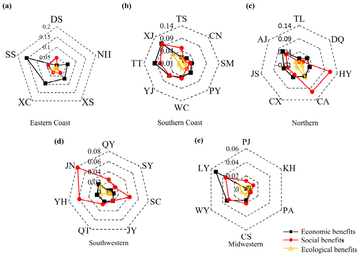
Figure 8 presents simulated land use benefit improvements across Zhejiang following county-level industrial structure optimization. All counties registered gains. Eastern coastal areas—notably SS (0.147), XC (0.09), and XS (0.05)—recorded the strongest economic improvements, averaging a 0.07 increase, outperforming social (0.03) and ecological (0.01) gains. The southern coastal region exhibited multidimensional progress, with counties like XJ (0.12, 0.09, 0.04) and TT (0.10, 0.09) achieving high-value, balanced development. Others, including YJ, WC, showed coordinated growth in at least two benefit categories. The south’s average ecological benefit increase was nearly 53% higher than the east’s, indicating a more balanced model. Northern regions led in social benefit growth (avg. 0.06), driven by CA (0.10) and HY (0.11). The midwestern and southwestern regions of Zhejiang saw improvements across all three benefit dimensions, with the southwestern region recording a notable rise in social benefits.

6. Conclusions

Optimizing industrial structure is crucial for regional development; while past research focused on macro input–output, this study explores internal dynamics: investment, employment, and output over time. An evaluation system reveals developmental status and evolutionary traits by analyzing response mechanisms. Importantly, a multi-objective optimization model, integrating economic, social and environmental benefits with an improved genetic algorithm, moves beyond single-objective economic models. Applied to 33 Zhejiang counties, it offers targeted strategies for industrial adaptation to boost land use benefits.

6.1. Evolutionary Characteristics of LUB and ISE from 2000 to 2020

Land use economic and social benefits follow an east-high and west-low spatial gradient, while ecological benefits show the opposite pattern with high values in inland areas and low values in northern coastal zones. The spatial clustering patterns of all three benefit dimensions are robust across different K-nearest-neighbor spatial weight matrices. The province underwent a marked sectoral shift. The primary sector contracted sharply in output (20% to 5%) and employment (40% to 20%). The secondary sector declined post-2010 but remained the largest employer (median 40%), with falling investment (60% to 30%). The tertiary sector became dominant, contributing over half the output and seeing a surge in investment (around 70%). This transition aligns with classical theories [55], yet county-level analysis reveals significant heterogeneity in pace and structure, alongside persistent challenges like inefficient investment, uneven industrial employment, and lagging agricultural modernization.

6.2. Targeted Strategies in Industrial Structure Optimization

This study identifies the inherent differences between two modes of unregulated service-sector expansion. Rodrik’s (2016) theory of premature deindustrialization illustrates that low-income economies with weak industrial bases witness a steady drop in secondary industry investment shares before full industrialization, alongside unruly growth of low-end services that distorts the whole industrial transformation process [56]. As an affluent coastal province in China, Zhejiang has entered the post-industrial era overall. Still, some counties ignore their local manufacturing foundations and overinvest in real estate and low-end cultural tourism. Insufficient producer service support thus triggers inefficient service expansion and distorted capital allocation at the county level. Recent cutting-edge studies focusing on China’s Yangtze River Delta also verify such regional heterogeneity [57,58]. Counties along the coast frequently suffer from identical service investment and skewed industrial ratios. Many local governments inflate their service sectors by relying on land finance, leaving a severe shortage of producer services and hindering the upgrading of manufacturing value chains. For counties that recklessly expand low-end services without solid manufacturing backing, authorities should set differentiated access thresholds for service investment matching local industrial endowments and adopt classified regulation to rationalize industrial composition.

Secondary-sector investment displays an inland deficit-coastal surplus pattern, while primary-sector deviations are minimal (<2.8%). Employment optimization reveals an industrial surplus coexisting with a tertiary sector deficit in eastern coastal and northern counties. Central-western and southwestern regions require agricultural labor transfer, industrial enhancement, and service-sector development. Southern coastal counties need targeted policies due to diversified structures. The main output optimization challenge is the secondary industry’s spatial imbalance: inland counties need manufacturing augmentation, while coastal areas require customized adjustments based on local deviation patterns.

6.3. Enhanced Benefits from Optimization

Simulation results indicate that county-level differentiated industrial optimization substantially improved land use benefits across all counties. These broad findings are largely consistent with Liu et al. [59], who find that province-level optimization of industrial structure (especially upgrading + rationalization) significantly increases urban land use benefits in China. However, our county-level results show much greater regional variation, emphasizing the need for finer spatial resolution. Eastern coastal areas realized an average economic benefit of 0.07. Southern coastal regions achieved multidimensional coordinated development, simultaneously advancing economic, social, and ecological benefits. Northern regions observed a breakthrough in social benefits, with an average increase of 0.06. Furthermore, central-western and southwestern regions exhibited steady, incremental improvements across all three dimensions, signifying their potential for robust sustainable development. This study provides theoretical and practical support for promoting rational industrial development and maximizing land use benefits.

6.4. Limitations

This study adopts the entropy weight method to assign objective weights based on data dispersion and fills missing data for certain years via linear interpolation, which introduces certain errors in measurement and evaluation results. In terms of sample selection, this study conducts a county-level empirical analysis in only one province. Although this effectively avoids interference caused by complex and inconsistent data definitions and policy systems across provinces and enables a precise focus on the actual association patterns between industrial structure and land use benefits at the county level, this sampling approach also has certain limitations. Moreover, to ensure consistent definitions and stable research units for the long-time-series analysis, the study did not include municipal districts created through county-to-district conversion or other administrative boundary adjustments. Therefore, the conclusions of this study apply only to county-level units with stable administrative divisions, and their generalizability and broader applicability are subject to certain constraints. It should also be clarified that this study mainly centers on economic sustainability, which is one core dimension of overall sustainability.

Future research can address these limitations in two ways: first, by improving the methodological framework and replacing static regression models with dynamic econometric models; and second, by refining the sampling framework, establishing a separate analytical system for municipal districts, harmonizing the statistical definitions of urban time-series data, and further enriching the research findings and expanding the applicability and generalizability of the conclusions.

References

1. Liu, H.F.; Bi, R.T. Research on externality and social benefits of collective profit-oriented construction land transfer: An empirical analysis of Zezhou County, Shanxi Province. Soft Sci. 2017, 31, 90–94. [Google Scholar] [CrossRef]
2. Zhuang, L.; Ye, C. Changing imbalance: Spatial production of national high-tech industrial development zones in China (1988–2018). Land Use Policy 2020, 94, 104512. [Google Scholar] [CrossRef] [Scilit]
3. Arndt, H.W. Colin Clark as a development economist. World Dev. 1990, 18, 1045–1050. [Google Scholar] [CrossRef] [Scilit]
4. Aspromourgos, T. On the origins of classical economics: Distribution and value from William Petty to Adam Smith. Cap. Cl. 1998, 22, 142–143. [Google Scholar] [CrossRef] [Scilit]
5. Kuznets, S. Economic Growth of Nations: Total Output and Productive Structure; Harvard University Press: Cambridge, MA, USA, 1971. [Google Scholar] [CrossRef] [Scilit]
6. Fagerberg, J. Technological progress, structural change and productivity growth: A comparative study. Struct. Change Econ. Dyn. 2000, 11, 393–411. [Google Scholar] [CrossRef] [Scilit]
7. Knudsen, D.C. Shift-share analysis: Further examination of models for the description of economic change. Socio-Econ. Plan. Sci. 2000, 34, 177–198. [Google Scholar] [CrossRef] [Scilit]
8. Feng, M. Global industrial transfer and upgrading China’s industrial structure level. Manag. World 2009, 5, 172–173. [Google Scholar] [CrossRef]
9. Ye, Q.L.; Duan, L.L.; Zhu, W.X. Measurement and influencing factors of China’s exhibition industry structure level. Stat. Decis. 2022, 38, 67–71. [Google Scholar] [CrossRef]
10. Zhou, D.; Cheng, H.P. Distribution dynamics and spatial dependence of China’s industrial structure level. Econ. Surv. 2015, 32, 79–84. [Google Scholar] [CrossRef]
11. Acemoglu, D.; Guerrieri, V. Capital deepening and nonbalanced economic growth. J. Political Econ. 2008, 116, 467–498. [Google Scholar] [CrossRef] [Scilit]
12. Foellmi, R.; Zweimüller, J. Structural change, Engel’s consumption cycles and Kaldor’s facts of economic growth. J. Monet. Econ. 2008, 55, 1317–1328. [Google Scholar] [CrossRef] [Scilit]
13. Li, H.M.; Yang, X.; Wu, X.L.; Jia, Y.H. Carbon emission effects of industrial structure evolution in energy-intensive industries from a spatio-temporal perspective. Acta Sci. Circumstantiae 2021, 41, 2018–2028. [Google Scholar] [CrossRef]
14. Gou, L.M. Measurement of the speed of transformation and upgrading of China’s industrial structure, spatio-temporal evolution and influencing factors. J. Ind. Technol. Econ. 2022, 41, 59–67. [Google Scholar] [CrossRef]
15. Kang, K.; Guo, P. Spatial characteristics and influencing factors of urban industrial structure distortion in China. Stat. Decis. 2023, 39, 120–124. [Google Scholar] [CrossRef]
16. Baffour Awuah, K.G.; Hammond, F.N.; Lamond, J.E.; Booth, C. Benefits of urban land use planning in Ghana. Geoforum 2014, 51, 37–46. [Google Scholar] [CrossRef] [Scilit]
17. Deines, J.M.; Schipanski, M.E.; Golden, B.; Zipper, S.C.; Nozari, S.; Rottler, C.; Guerrero, B.; Sharda, V. Transitions from irrigated to dryland agriculture in the Ogallala Aquifer: Land use suitability and regional economic impacts. Agric. Water Manag. 2020, 233, 106061. [Google Scholar] [CrossRef] [Scilit]
18. Yang, L.X.; Xia, H.; Yuan, S.F. Based on coupling coordination degree analysis of spatial differences in land use economic efficiency: A case study of Zhejiang Province. China Land Sci. 2015, 29, 83–88. [Google Scholar]
19. Cai, L.J. Research on the coupling mechanism and linkage path of rural tourism and rural land use economic benefit. Agric. Econ. 2016, 3, 51–52. [Google Scholar]
20. He, K. Economic benefit analysis of urban land use in China based on scale. Rural Econ. Sci.-Technol. 2021, 32, 51–54. [Google Scholar]
21. Chen, S.Y.; Chen, A.Z.; Zhou, F. Study on social benefits and spatio-temporal characteristics of regional land use. Resour. Dev. Mark. 2008, 11, 975–978. [Google Scholar]
22. Lin, Y.F. Industrial policy and China’s economic development: A perspective of new structural economics. Fudan Univ. J. (Soc. Sci.) 2017, 2, 148–153. [Google Scholar]
23. Zhou, K.; Wang, F.H. Study on social benefit evaluation of land use system: A case study of Banan District, Chongqing. China. Popul. Resour. Environ. 2017, 27, 166–169. [Google Scholar] [CrossRef] [Scilit]
24. Daily, G.C. Nature’s Services: Societal Dependence on Natural Ecosystems; Island Press: Washington, DC, USA, 1997. [Google Scholar] [CrossRef] [Scilit]
25. Costanza, R.; de Groot, R.; Sutton, P.; van der Ploeg, S.; Anderson, S.J.; Kubiszewski, I.; Farber, S.; Turner, R.K. Changes in the global value of ecosystem services. Glob. Environ. Change 2014, 26, 152–158. [Google Scholar] [CrossRef] [Scilit]
26. Brauman, K.A.; Daily, G.C.; Duarte, T.K.; Mooney, H.A. The nature and value of ecosystem services: An overview highlighting hydrologic services. Annu. Rev. Environ. Resour. 2007, 32, 67–98. [Google Scholar] [CrossRef] [Scilit]
27. Luo, P.; Zhou, S. Impact of land use change on ecological benefits in suburban agricultural areas: A case study of Gaoping District of Nanchong City, Sichuan Province. J. Ecol. Rural Environ. 2007, 4, 6–10. [Google Scholar]
28. Sun, L.; Zhang, B.; Zhang, J.; Jin, S.; Ma, Z. Inland river basin land use/cover change ecological benefit evaluation: A case study of the middle and lower reaches of the Shule River. Arid. Land Resour. Environ. 2013, 27, 80–85. [Google Scholar] [CrossRef]
29. Wang, J.; Wei, Z. Analysis on eco-environmental benefits under different land use patterns in the west dump of Fushun West Open-pit Mine. China Land Sci. 2012, 26, 74–79. [Google Scholar] [CrossRef]
30. Cui, D.; Song, G. Research on land ecological benefit evaluation of coal cities in Heilongjiang Province: A case study of Hegang City. Bull. Soil Water Conserv. 2010, 17, 114–117. [Google Scholar]
31. Yan, Y.; Lei, G.; Xie, Y. Research on land use ecological benefit based on AHP and entropy weight method. Bull. Soil Water Conserv. 2014, 21, 134–139. [Google Scholar] [CrossRef]
32. Chu, Z.; Xu, C.; Luo, Y.; Sun, Q. Land use simulation and ecological benefit evaluation in the Tarim River Basin based on ecological protection red line management. Acta Ecol. Sin. 2021, 41, 7380–7392. [Google Scholar] [CrossRef] [Scilit]
33. Guo, X.; Chang, Q.; Liu, X.; Bao, H.; Sun, Y.; Lv, C.; Zhang, Y. Urban land use patterns and ecological benefit differentiation from a carbon storage perspective. China Land Sci. 2017, 31, 61–70. [Google Scholar] [CrossRef]
34. Lu, C.; Yang, Q.; Jin, D.; Li, X.; Wen, F. An empirical study on the correlation between urban land use structure and industrial structure: A case study of Chongqing. Urban Dev. Stud. 2010, 1, 102–107. [Google Scholar]
35. Lu, X.; Jiang, X.; Gong, M. How land transfer marketization influence on green total factor productivity from the approach of industrial structure? Evidence from China. Land Use Policy 2020, 95, 104610. [Google Scholar] [CrossRef] [Scilit]
36. Dan, C.; Xiong, H. Research on the relationship between land use structure and industrial development in Hainan. Resour. Sci. 2010, 32, 718–723. [Google Scholar]
37. Zhang, H.; Ju, Z.; Zhang, F. Correlation analysis between socio-economic structure and land use structure changes in China. China Land Sci. 2007, 21, 12–17. [Google Scholar] [CrossRef]
38. Cao, Z.; Hao, J.; Guo, L. Strategic model discussion on industrial and land spatial agglomeration development in the Huang-Huai-Hai region. Resour. Sci. 2010, 32, 2145–2151. [Google Scholar]
39. Yin, Y.; Liu, Z.; Dunford, M.; Liu, W. The 798 Art District: Multi-scalar drivers of land use succession and industrial restructuring in Beijing. Habitat Int. 2015, 46, 147–155. [Google Scholar] [CrossRef] [Scilit] [PubMed]
40. Yang, Y.; Jiang, G.; Zheng, Q.; Zhou, D.; Li, Y. Does the land use structure change conform to the evolution law of industrial structure? An empirical study of Anxi Province, China. Land Use Policy 2019, 81, 657–667. [Google Scholar] [CrossRef] [Scilit]
41. Zhang, Y.; Wang, Q.; Wang, W. An empirical study on the interrelationship between industrial structure and land use structure in China. China Land Sci. 2007, 21, 4–11. [Google Scholar] [CrossRef]
42. Zhang, Q.; Li, J. Analysis of the relationship between land use structure and economic structure in Handan City. J. Hebei Norm. Univ. (Nat. Sci.) 2000, 24, 129–132. [Google Scholar] [CrossRef]
43. Jin, Q.; Deng, X.; Wang, Z.; Shi, C.; Li, X. Analysis and projection of the relationship between industrial structure and land use structure in China. Sustainability 2014, 6, 9343–9370. [Google Scholar] [CrossRef] [Scilit]
44. Meng, Y.; Zhang, F.; Jiang, G.; Chen, T. Study on the relationship between industrial structure and land use structure in Beijing. Areal Res. Dev. 2011, 30, 108–111. [Google Scholar]
45. Ma, A.; Li, C.; Liu, S. Study on the coupling relationship between urban industrial structure and land use: A case study of Shenyang City. J. Shanxi Univ. Financ. Econ. 2012, 34, 29–31. [Google Scholar] [CrossRef]
46. Fan, S.; Liu, Y.; Zhang, H.; Hou, C.; Chang, D. Spatial suitability evaluation of land for undertaking transferred industries based on hierarchical fuzzy matter-element model. Trans. Chin. Soc. Agric. Eng. 2015, 31, 266–276. [Google Scholar]
47. Wu, Y.; Zhou, C.; Lai, X.; Li, Y.; Miao, L.; Yu, H. Spatio-temporal characteristics and decoupling relationship of new-type urbanization and carbon emissions at the county Level: A case study of Zhejiang Province, China. Ecol. Indic. 2024, 160, 111793. [Google Scholar] [CrossRef] [Scilit]
48. Zhu, X.; Zhang, P.; Wei, Y.; Li, Y.; Zhao, H. Measuring the efficiency and driving factors of urban land use based on the DEA method and the PLS-SEM model—A case study of 35 large and medium-sized cities in China. Sustain. Cities Soc. 2019, 50, 101646. [Google Scholar] [CrossRef] [Scilit]
49. Wang, G.; Liu, Y.; Fang, F. Comprehensive measurement and spatial differentiation of land use benefits in the Bohai Rim region. Prog. Geogr. 2013, 32, 649–656. [Google Scholar] [CrossRef]
50. Cui, M. Eco-environmental effects of industrial structure evolution in Anhui Province. Econ. Geogr. 2020, 40, 131–137. [Google Scholar] [CrossRef]
51. Jiao, H.; Yang, X. Coupling relationship between industrial structure evolution and spatial form evolution in coal resource-based cities: A case study of Huainan City in Anhui Province. Acta Geogr. Sin. 2016, 71, 998–1009. [Google Scholar] [CrossRef]
52. Jiang, M.; Zhao, P. Research on the impact of industrial land structure on production space utilization efficiency: Based on the perspective of land price ratio imbalance and industrial upgrading. Nankai Econ. Stud. 2025, 1, 162–182. [Google Scholar] [CrossRef]
53. Lu, J.; Fang, B.; Li, X. Research on the optimal intensity of land use in Jiangsu Province based on Pareto optimality. Chin. J. Agric. Resour. Reg. Plan. 2019, 40, 136–145. [Google Scholar]
54. Wang, H.Y.; Gao, P.C.; Xie, Y.R.; Song, C.Q.; Cheng, C.X.; Ye, S.J. Multi-objective optimization of land use in Xining City based on improved NSGA-II. Geogr. Geo-Inf. Sci. 2020, 36, 84–89. [Google Scholar] [CrossRef]
55. Herrendorf, B.; Rogerson, R.; Valentinyi, Á. Growth and structural transformation. Handb. Econ. Growth 2014, 2, 855–941. [Google Scholar] [CrossRef] [Scilit]
56. Rodrik, D. Premature deindustrialization. J. Econ. Growth 2016, 21, 1–33. [Google Scholar] [CrossRef] [Scilit]
57. Fang, P.; Cao, X.; Huang, Y.; Chen, Y. How Does the Platform Economy Affect Urban System: Evidence from Business-to-Business (B2B) E-Commerce Enterprises in China. Buildings 2025, 15, 1687. [Google Scholar] [CrossRef] [Scilit]
58. Fang, P.; Wang, Z.; Huang, Y.; Chen, Y.; Cao, X. Administrative Fragmentation and Functional Integration: Quantifying Urban Interstice Dynamics in Jurong Using Mobile Origin–Destination (OD) Flows. Appl. Sci. 2025, 15, 5675. [Google Scholar] [CrossRef] [Scilit]
59. Liu, J.; Hou, X.; Wang, Z.; Shen, Y. Study the effect of industrial structure optimization on urban land-use efficiency in China. Land Use Policy 2021, 105, 105390. [Google Scholar] [CrossRef] [Scilit]
Figure 1. Location and study area. (This figure is based on the standard map service website of the Ministry of Natural Resources with the map approval number of GS (2019)1651).
Sustainability 18 07555 g001
Figure 2. Methodological framework.
Sustainability 18 07555 g002
Figure 3. Temporal evolution of Global Moran’s I for county−level economic, social, and ecological benefits. The dashed horizontal line denotes the expected value under spatial randomness. *, **, and *** denote permutation-test significance at p < 0.05, p < 0.01, and p < 0.001, respectively; ns denotes non-significance.
Sustainability 18 07555 g003
Figure 4. Moran scatter plots for economic (ac), social (df), and ecological (gi) benefits in 2000, 2010, and 2020. The slope of the fitted line equals Global Moran’s I. Red and blue points denote significant high−high and low−low counties, respectively; gray points denote spatial outliers or non-significant counties. *** denotes permutation-test significance at p < 0.001; ns denotes non-significance.
Sustainability 18 07555 g004
Figure 5. LISA cluster maps for county–level economic (ac), social (df), and ecological (gi) benefits in 2000, 2010, and 2020. Hatched polygons indicate counties without study data and are not included in the spatial-statistical calculations.
Sustainability 18 07555 g005
Figure 6. Evolution of the investment (ac), employment (df), and output (gi) structures of primary, secondary, and tertiary industries in county-level regions of Zhejiang Province, 2000–2020.
Sustainability 18 07555 g006
Figure 7. The response degree of land use benefit to industrial structure evolution: (a) Eastern Coast and Northern Zhejiang; (b) Southern Coast and Midwestern Zhejiang; (c) Southwestern Zhejiang.
Sustainability 18 07555 g007
Figure 8. Simulated optimization gains in economic, social and ecological benefits across county−level regions of Zhejiang Province: (a) Eastern Coast; (b) Southern Coast; (c) Northern Zhejiang; (d) Southwestern Zhejiang; (e) Midwestern Zhejiang.
Sustainability 18 07555 g008