CFD-Based Analysis of Construction Dust Dispersion and the Height-Dependent Performance of Dust Control Fences in Surrounding Environments

Abstract

Construction dust is a major contributor to urban inhalable particulate matter (PM₁₀) pollution, posing severe respiratory and cardiovascular health risks to construction workers and nearby residents, severely undermining urban environmental sustainability. Construction fences are widely adopted as a primary dust mitigation measure, yet their underlying dispersion mechanisms and comprehensive impacts on vertical air quality remain poorly understood due to the limitations of traditional field monitoring and empirical models, creating critical barriers to site-level pollution control and long-term urban sustainability. In this study, a reliable computational fluid dynamics (CFD) method was developed to investigate the spatial distribution of construction dust and quantify the dust suppression performance of fences with heights ranging from 0 to 3 m. Three mainstream k-ε turbulence models (Standard, RNG, and Realizable) were evaluated using on-site measurement data, and the RNG k-ε model was found to provide the best agreement with field observations, with statistical metrics of q = 1, FB = 0.052, and NMSE = 0.028. The results show that construction fences effectively reduce dust dispersion into the surrounding environment, particularly in the pedestrian breathing zone (z < 1.5 m). Increasing the fence height from 1.5 m to 3 m improves the breathing-zone dust reduction rate from 39% to 55%, with the most significant mitigation effect observed within 50 m downwind of the fence. However, a critical dual effect was identified: while fences suppress near-ground pollution, they induce strong upward airflow and turbulence, leading to elevated dust concentrations in the upper part of the near-ground region (z = 1.5–9 m), a phenomenon absent in the no-fence scenario. These findings provide practical implications for urban construction site management, suggesting that fence height and configuration should be carefully designed not only to reduce pedestrian-level exposure but also to avoid unintended pollutant accumulation aloft, thereby improving overall air quality control strategies and delivering balanced, long-term environmental sustainability at construction sites.

1. Introduction

Construction dust, generated during building and infrastructure development, has become a globally recognized contributor to urban air pollution, particularly in the form of inhalable particulate matter (PM10) [1,2,3,4], threatening urban ecological health and long-term urban sustainability. The rapid expansion of construction activities has led to frequent exceedances of PM10 limits in many cities around the world [5,6,7,8]. In China, for instance, in 2025 the total floor area under construction has exceeded 6.6 billion m² and continues to rise [9], contributing significantly to dust emissions and related health risks. The World Health Organization (2021) [10] reported that PM10 from construction dust will lead to increased risks of respiratory and cardiovascular diseases. Every 10 μg/m³ increase in PM10 concentration is associated with a 7.2% rise in overall morbidity, with 47.4% of the cases involving respiratory illness, 38.2% cardiovascular conditions, and 14.4% other systemic health effects [11]. Field studies in different cities, such as those by Keer et al. [12] in New Zealand and Azarmi et al. [13] in London, have consistently shown that construction workers and nearby residents are exposed to serious health risks due to dust pollution. Notably, construction workers directly exposed to dust experience the most pronounced symptoms, including higher rates of wheezing and chronic cough [14,15]. Therefore, a deeper understanding of construction dust dispersion mechanisms is crucial for developing effective control strategies, ultimately contributing to improved urban air quality, equitable public health protection, and robust environmental sustainability.

Current studies on construction dust have primarily focused on field monitoring [16,17,18] and empirical models [19,20,21], and their aims were to analyze the emission characteristics, composition, and pollution patterns of construction dust. For example, Liu et al. [22] conducted on-site measurements of dust distribution during the demolition phase of a construction site, analyzing the concentration distribution of inhalable particulate matter (PM10). The emission factor method, as a simpler and more direct empirical approach, has been widely applied in large-scale regional pollutant emission estimations. Muleski et al. [23] performed detailed measurements of particulate matter emissions from various construction activities, such as earthworks, truck loading and unloading, and soil and mud tracking, and provided corresponding PM10 and PM2.5 emission factors for different activities. However, field monitoring is limited by the number and placement of sensors, as well as the measurement accuracy, so it is difficult to fully capture the spatial distribution of the dust. Although the empirical models offer computational efficiency, they rely on generalized parameters and often produce rough estimates that do not accurately reflect on-site conditions. More importantly, both of these methods are unable to reveal the detailed dispersion processes of construction dust and the effects on the air quality in the surrounding environment.

Computational fluid dynamics (CFD) has been widely employed to simulate air flow and particulate dispersion in different flow conditions due to its relatively low cost and high spatial-temporal resolution. It has been successfully used in modeling vehicle exhaust dispersion [24,25,26] and atmospheric particulate transport in urban areas. For example, Dyck & Stukel [27] used CFD to quantify dust emissions on unpaved construction roads, and revealed the relationships between vehicle speed, vehicle weight, and road surface dust accumulation. In addition, Wang et al. [28] and Cai et al. [29] also employed CFD to investigate coal dust transport in enclosed or semi-enclosed environments. Although these studies focused on confined spaces that differ from the open atmospheric conditions of urban construction sites, the findings particularly regarding how particulate matter is transported in turbulent flows still offer important methodological references for modeling construction dust dispersion. Thus, the CFD method has great potential for analyzing the spatial distribution of construction dust, an aspect that remains insufficiently addressed in current studies.

On the other hand, windbreak fences have been proven effective in suppressing dust transport in settings like ports, coal storage facilities, and desert railway systems [30,31]. For instance, Raine & Stevenson [32] found that fences suppress dust primarily by reducing incoming wind speed. Similarly, Kim et al. [33] employed CFD simulations to analyze dust dispersion over reclaimed land. However, these studies mainly focused on natural surfaces or industrial dust sources, with limited relevance to urban construction sites. Although construction fences are widely employed in cities as a dust mitigation measure, the actual impact of the fences on dust dispersion patterns has not been evaluated so far. In particular, the interaction between construction fences and surrounding airflow structures, especially the induced vertical transport and upper-layer accumulation of pollutants, has not been systematically quantified in previous research. Third, existing studies on windbreak fences mainly target natural terrain or industrial stockpiles, which differ significantly from urban construction environments in terms of geometry and flow complexity.

The main objectives of this study were to (1) establish a reliable CFD numerical method, validated by field measurements, for investigating the spatial distribution patterns of construction dust, and (2) to assess the dust suppression effectiveness of construction fences with different heights. The results of this study show that construction fences effectively reduce the pollutant concentrations in the breathing zone of the surrounding environment. However, the fences also lead to pollutant accumulation in the upper-level region. Future research should aim to optimize fence designs to improve overall dust control ability while minimizing adverse effects in upper atmospheric regions, creating integrated mitigation solutions that align with long-term urban environmental sustainability targets.

2. Methodology

2.1. Model

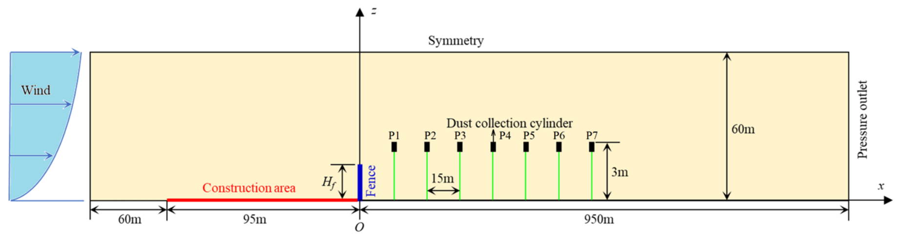
To simulate the dispersion of pollutants from the construction site into the downstream region, as shown in Figure 1, a simplified two-dimensional (2D) model based on a real construction case (the National Aquatics Center construction site in Beijing) is employed as the computational domain [18]. This is because the primary research objective is to evaluate the reduction pattern of dust concentration due to the shielding effect of construction fences under typical wind-driven dispersion conditions, and the construction sites are usually wide enough, and the construction fences are often continuously arranged along the site boundary. Under such conditions, the airflow and dust dispersion in the lateral direction can be reasonably assumed to be uniform, so a representative 2D vertical section (x–z plane) in the middle of the site is selected for the present simulation.

The parameters of this construction site are well-documented, and during the experimental period, the surrounding area consisted of relatively open bare land covered with large amounts of Artemisia grass, with minimal human interference [18]. This means there are no obstructions (such as buildings) to strongly deflect or disturb the airflow, and the low Artemisia grass had little effect on the wind fields. These characteristics facilitate the numerical reproduction of the spatial distribution and dispersion process of construction dust while allowing for an isolated evaluation of the impact of construction fences, minimizing the influence of other secondary factors.

The construction site (marked by the red line, x = 95 m~0) has a length of 95 m. To effectively separate the construction and non-construction areas and mitigate dust pollution in the surrounding environment, particularly in the downwind region, a construction fence (marked by the blue line at x = 0) was placed at the downstream boundary of the site, with H_f = 2 m.

During the mid-stage of construction (November 2004), multiple measurement points (P1 to P7, see Figure 1) were evenly distributed within a 100 m range downwind of the fence at 15 m intervals, with a measurement height of 3 m. Particulate matter (PM₁₀) concentrations were measured using a TSI DustTrak aerosol monitor [18]. A medium-volume PM sampler equipped with a PM₁₀ inlet and quartz fiber filters was used as a gravimetric reference instrument. Both instruments were colocated and operated simultaneously. Filter samples were collected at 1-h intervals over a 12-h period. After sampling, filters were sealed and stored in a desiccator, then conditioned under controlled temperature and humidity before weighing. Gravimetric results were used to calibrate the DustTrak data.

This study first reconstructed the dust concentration distribution at the construction site with a 2 m-high fence through numerical simulation and compared the results with field measurements. Once the numerical methodology was validated, the study further evaluated the dust suppression effectiveness of the fence and analyzed the impact of different fence heights (H_f) on the spatial dispersion characteristics of construction dust. Given that construction fence heights generally do not exceed 3 m, five cases (H_f = 0 (no fence), 1.5 m, 2 m, 2.5 m, and 3 m) were considered for analysis.

To mitigate the adverse effects of computational domain boundaries [34,35,36], a transition section and a wake development region were added to the computational domain, as shown in Figure 1. The upstream transition section was set to 60 m, while the wake development region extended 950 m downstream, equivalent to 10 times the length of the construction site. The total domain height was set to 20 times the maximum fence height (H_f(max) = 3 m), resulting in a domain height of 60 m.

The left boundary of the computational domain was set as a velocity inlet, the right boundary as a pressure outlet, while the fence and ground were treated as wall boundaries. The top boundary of the domain was assigned a symmetry condition.

Wind speed in the atmospheric boundary layer varies with height and is commonly modeled using the power-law distribution [36,37]:

$$U_z=U_{ref}{({\displaystyle \frac{z}{Z_{ref}}})}^r$$

(1)

where U_z represents the wind speed at height z, while U_ref, Z_ref, and r denote the reference wind speed, reference height, and ground roughness exponent, respectively. The roughness exponent r depends on surface characteristics, with rougher terrain exerting a stronger resistance to airflow [38,39]. According to the Chinese Load Code [37], terrain is classified into four categories: A (ocean), B (rural), C (urban), and D (city center), with corresponding r values of 0.12, 0.15, 0.22, and 0.3. Given that the layout around the construction site during the study period was close to the rural area, a roughness index r = 0.15 was used in this study. The nearest meteorological station to the construction site (Haidian District, Beijing, Station No. 54511) has recorded the average monthly wind speed of 2.2 m/s at the height of 31.3 m during the construction period, which was adopted as the inlet wind speed in the present CFD simulation [40]. Therefore, Z_ref = 31.3 m, U_ref = 2.2 m/s. In addition, it is acknowledged that both very high and very low wind speeds correspond to low-frequency extreme meteorological conditions and therefore cannot adequately represent the long-term typical ventilation and pollutant dispersion characteristics of the study area. Using a long-term mean wind speed (i.e., U_ref = 2.2 m/s) allows the simulations to capture a statistically representative flow regime, which is commonly adopted in urban microclimate and dispersion studies for assessing typical exposure conditions.

The turbulence characteristics of the inlet wind were modeled using the turbulence intensity equation, turbulent kinetic energy (k_z) and its dissipation rate (ε_z) [37]:

$$I_z=I_{10}{({\displaystyle \frac{z}{10}})}^{-r}$$

(2)

$$k_z=1.0{(U_z{I}_z)}^2$$

(3)

$${\epsilon }_z={\displaystyle \frac{C_{\mu }{{}^{0.75}k_z}^{1.5}}{I_z}}$$

(4)

where I_z represents the turbulence intensity at height z, and I₁₀ is the turbulence intensity at 10 m above ground. The value of I₁₀ depends on terrain classification, with values of 0.12, 0.14, 0.23, and 0.39 for categories A, B, C, and D, respectively [37]. As mentioned above, the layout of the construction site during the study period was close to the rural area, so a value of I₁₀ = 0.14 was adopted in this study. C_µ = 0.0845 is the constant of the RNG k-ε turbulence model.

2.2. Numerical Methodology

The numerical simulations in this study were conducted using ANSYS FLUENT 2024R1. The second-order upwind scheme was used to discretize the above equations [41,42], and for pressure–velocity coupling, the SIMPLE algorithm was adopted [43]. Construction dust generated during building activities interacts with the wind field in an open environment, forming a typical gas–solid two-phase flow system. The most commonly used numerical method for gas–solid flow modeling combines a continuous gas model with a discrete particle model (DPM), in which the gas is the continuous phase while the particles are treated as the discrete phase. Such a model is particularly suited for environments with low particle concentrations. Considering that the construction dust particles have a low volumetric loading and are dispersed in the open atmospheric boundary layer, the continuous gas model with the DPM was adopted to simulate dust particle behavior in this study [44,45,46].

To obtain the spatial distribution of particles, it is first necessary to establish a steady-state flow field. Given that a construction site is an open environment, the density of air does not significantly change as airflow passes through [47,48]. Thus, to simplify the calculations, the airflow in the computational domain was assumed to be steady, isothermal, and incompressible turbulent flow.

The presence of the construction fence significantly influences the wind field, altering airflow velocity and direction, generating local turbulence and airflow recirculation, and consequently affecting the dispersion and spatial distribution of dust particles. The RNG k-ε model was selected for turbulence modeling as it provides improved accuracy in capturing turbulence effects, thereby enhancing the reliability of the computational results [49]. The governing equation for turbulence is as follows:

$$\nabla \cdot \mathit{u}=S_m$$

(5)

$$\mathit{u}\cdot \nabla \mathit{u}=-{\displaystyle \frac{1}{\rho }}\nabla p+{\displaystyle \frac{1}{\rho }}\nabla \cdot (\mu (\nabla \mathit{u}+{(\nabla \mathit{u})}^T))+\mathit{g}+\mathit{F}$$

(6)

$$\mathit{u}\cdot \nabla k={\displaystyle \frac{1}{\rho }}\nabla \cdot ({\sigma }_k{\mu }_{eff}\nabla k)+{\displaystyle \frac{1}{\rho }}{P}_k-\epsilon +S_k$$

(7)

$$\mathit{u}\cdot \nabla \epsilon ={\displaystyle \frac{1}{\rho }}\nabla \cdot ({\sigma }_{\epsilon }{\mu }_{eff}\nabla \epsilon )+C_{\epsilon 1}{\displaystyle \frac{\epsilon }{\rho k}}{P}_k-C_{\epsilon 2}{\displaystyle \frac{{\epsilon }^2}{k}}-R_{\epsilon }+S_{\epsilon }$$

(8)

$$R_{\epsilon }={\displaystyle \frac{C_{\mu }{\eta }^3(1-\eta /{\eta }_0)}{1+{\beta }_0{\eta }^3}}{\displaystyle \frac{{\epsilon }^3}{k}}$$

(9)

$$\eta ={\displaystyle \frac{k}{\epsilon }}{\left[({\displaystyle \frac{\partial u_i}{\partial x_j}}+{\displaystyle \frac{\partial u_j}{\partial x_i}}){\displaystyle \frac{\partial u_i}{\partial x_j}}\right]}^{1/2}$$

(10)

where C_ε1 = 1.44, C_ε2 = 1.68, σ_k = 0.7179, σ_ε = 0.7179, β₀ = 0.012, and η₀ = 4.377 are the closure constants. u represents the airflow velocity, and S_m represents the mass added to the continuous phase from the dispersed secondary phase [50,51], g is the gravitational acceleration, and F represents other body forces [52]. The parameter k represents the turbulent kinetic energy, ε is the turbulent dissipation rate, and µ_eff = µ + µ_t, µ_t = C_µ k²/ε is the turbulent eddy viscosity. P_k is the production of the turbulent kinetic energy. S_k and S_ε are additional source terms accounting for the influences of the dispersed phase on the turbulence of the continuous phase.

Once the velocity and pressure fields of the continuous phase for the entire computational domain were obtained, a force balance equation governing particle motion was established. This study focused on the dispersion characteristics of construction dust and the dust suppression effectiveness of fences, emphasizing the overall dust concentration rather than tracking individual particle trajectories, and since the volume fraction of the particle phase is relatively low, only drag force, gravitational force, and pressure gradient force were considered, while particle-particle collisions were neglected [53]. According to Newton’s Second Law, the governing equation for particle motion is:

$${\displaystyle \frac{d{\mathit{u}}_{pt}}{dt}}=\mathit{g}+{\mathit{F}}_d+{\mathit{F}}_p$$

(11)

$${\mathit{F}}_d={\displaystyle \frac{3}{4}}{C}_d{\displaystyle \frac{\rho }{{\rho }_{pt}}}(\mathit{u}-{\mathit{u}}_{pt})\left|u-{\mathit{u}}_{pt}\right|$$

(12)

$${\mathit{F}}_p=-\nabla p$$

(13)

where F_d is the drag force induced by particle-fluid interactions, F_p is the pressure gradient force caused by flow field non-uniformity, ρ is the air density, ρ_pt is the particle density, and u_pt is the particle velocity. The drag coefficient C_d, which depends on the particle Reynolds number Re_pt, is given by:

$$C_d=\left\{\begin{array}{ll}{\displaystyle \frac{24}{{\mathrm{Re}}_{\mathrm{pt}}}}(1+0.15{\mathrm{Re}}_{\mathrm{pt}}{}^{0.687})& {\mathrm{Re}}_{\mathrm{pt}}\le 1000\\ 0.43& {\mathrm{Re}}_{\mathrm{pt}}>1000\end{array}\right.$$

(14)

where the particle Reynolds number Re_pt is defined as:

$${\mathrm{Re}}_{\mathrm{pt}}={\displaystyle \frac{\rho d\left|\mathit{u}-{\mathit{u}}_{pt}\right|}{\mu }}$$

(15)

The motion of dust particles is influenced by both the airflow direction and turbulence fluctuations. To account for the effect of turbulence fluctuations on particle trajectories, the random walk model (stochastic tracking model) was applied.

It is important to clarify that the dust concentrations measured at the construction site represent the average dust deposition concentration over the entire (i.e., one-month) monitoring period, rather than the instantaneous release at a particular time or construction stage. Therefore, in the present CFD simulation, the dust particles were assumed to be uniformly emitted from the ground surface of the construction site (see Figure 1) with a mean mass flow rate of q = 1 × 10⁻⁵ kg/s [53]. Particles were assumed to be spherical, with an aerodynamic diameter of d = 10 µm, and no phase change or chemical reactions were considered. Furthermore, secondary dust resuspension was ignored, meaning that once dust particles impact the ground or the fence, they were considered captured. The details about the parameter settings of the numerical simulations in this study can be found in

Table 1. Parameter settings of the numerical simulations.

Object	Parameter	Settings
Solver	Solver	Pressure-based
	Steady/unsteady	Steady
	Turbulence model	RNG k-ε
	Algorithm	SIMPLE
	Discretization	Second order upwind
	Gravity acceleration	−9.8 m/s2
Boundary condition	Inlet	Velocity-inlet
	Outlet	Pressure-outlet
	Top	Symmetry
	Ground	No-slip wall
	Fence	No-slip wall
Discrete phase	Model	Discrete phase
	Group frequency/step	10
	Injection type	Surface
	Discrete random walk model	on
	Boundary trap of particle	on
	Density	1550 kg/m3
	Diameter	10 μm
	Total flow rate of the dust	1 × 10−5 kg/s

.

2.3. Model Validation

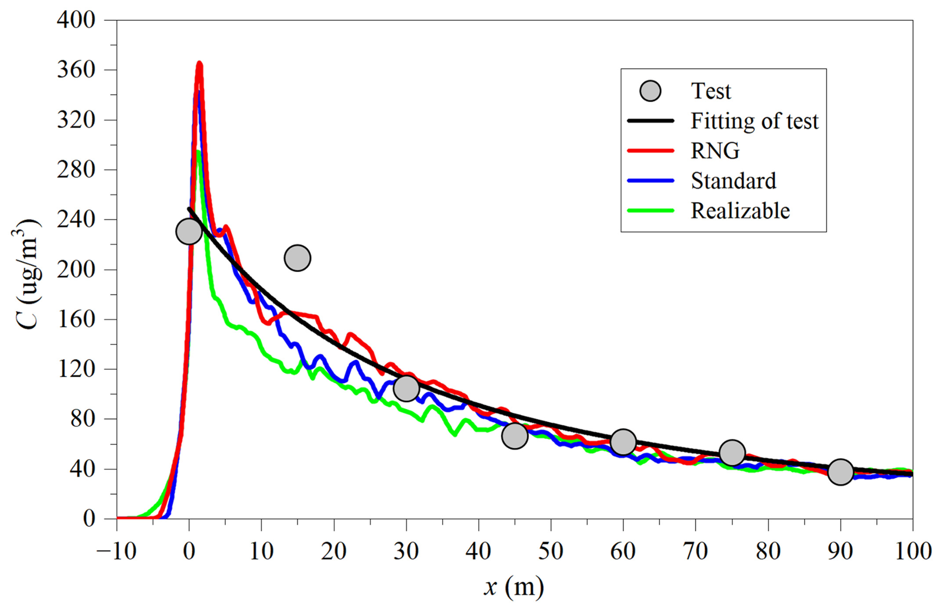
To ensure the reliability of the numerical simulation results obtained from the RNG k-ε turbulence model, the field measurement data from the construction site were used in this study [18]. As mentioned in Section 2.1, the construction fence height at the construction site is H_f = 2 m, and dust concentration measurements were conducted at a height of 3 m above the ground at 15 m intervals within a 100 m range downwind of the fence, as shown in Figure 1. In this study, in addition to the RNG k-ε model, the numerical results of the other two turbulence models, i.e., Standard and Realizable k-ε, were also provided as relevant supporting data to inform the selection of turbulence models. Figure 2 presents the comparison between the simulated and measured dust concentrations at P1 to P7 obtained from the three models. Note that the coordinate of P1 is x = 0. The detailed measured and simulated values at each sampling point are provided in

Table A1. Exact measured C, simulated C and relative error (E_i) for each specific monitoring point (P1 to P7).

Measurement Points		P1	P2	P3	P4	P5	P6	P7
Measured data	C (μg/m3)	230.5	209	105	66.5	61.5	53	37.5
RNG	C (ug/m3)	230.1	163.2	107.3	75	63.4	54.3	36
	Ei (%)	0.2	21.9	2.2	12.8	3.1	2.5	4
	q	1	1	1	1	1	1	1
Realizable	C (μg/m3)	230.3	140.2	102.7	75.3	56.5	42.3	36
	Ei (%)	0.1	32.9	2.2	13.2	8.1	20.2	4.0
	q	1	0	1	1	1	1	1
Standard	C (μg/m3)	230.4	122.3	85.3	75.5	56.2	41.6	40.3
	Ei (%)	0.0	41.5	18.8	13.5	8.6	21.5	7.5
	q	1	0	1	1	1	1	1

in the Appendix A.

As observed in Figure 2, the simulated dust concentration profiles from all three models exhibited a decay trend similar to that of the measured data, indicating good agreement. However, at approximately x = 15 m downwind of the fence, all three models underestimated the dust concentration compared to the measured data. This discrepancy may be caused by the well-known limitations of the RANS models, which tend to simplify vortex structures and recirculation zones behind obstacles [54,55,56]. This can lead to an overestimation of the recovery process of the wake region velocity, causing the pollutant dispersion ability to be overestimated, and thus resulting in lower concentrations than the observed values. Additionally, Figure 2 indicates that the RNG k-ε model provides the best agreement with the measured data, which may be due to the fact that the RNG model introduces an additional term in the ε equation derived from Renormalization Group (RNG) theory, enhancing its sensitivity to rapid strain and streamline curvature. Moreover, the RNG model also includes an eddy viscosity correction, which enables better performance in regions of low vorticity and recirculating flows [57,58,59].

To further quantify the agreement between simulation and field data, three statistical metrics were employed: Hit Rate (q), Fractional Bias (FB), and Normalized Mean Square Error (NMSE) [60,61,62]. The mathematical expressions for these metrics are:

$$q={\displaystyle \frac{1}{N}}{\displaystyle \sum _{i=1}^N{n}_i} \mathrm{with} n_i=\left\{\begin{array}{l}1 \mathrm{for} E_i\le E_r\hfill \\ 0 \mathrm{else} \hfill \end{array}\right.,E_i=100\%\times \left|{\displaystyle \frac{S_i-T_i}{T_i}}\right|$$

(16)

$$\mathrm{FB}=2{\displaystyle \frac{\overline{T}-\overline{S}}{(\overline{T}+\overline{S})}}$$

(17)

$$\mathrm{NMSE}={\displaystyle \frac{\overline{{\left(S_i-T_i\right)}^2}}{\overline{S}\cdot \overline{T}}}$$

(18)

where S_i and T_i represent the simulated and measured values, respectively, E_r = 25% is the allowable relative error, and the overline ‘−’ denotes the mean of the dataset. The acceptable ranges for these metrics are: q > 0.8, −0.3 ≤ FB ≤ 0.3, NMSE ≤ 1.5 [60,61,62]. For an ideal numerical model, q = 1, while FB = NMSE = 0.

Table 2. Overall accuracy assessment of turbulence models using three statistical metrics.

	RNG	Realizable	Standard
q	1	0.857	0.857
FB	0.052	0.109	0.161
NMSE	0.028	0.068	0.071

Note: Acceptable ranges are q ≥ 0.8, −0.3 ≤ FB ≤ 0.3, NMSE ≤ 1.5.

presents the overall accuracy assessment of the three turbulence models based on these statistical metrics. Please note that the statistical metrics are calculated based on raw monitoring data.

As shown in Table 2, the computed q, FB, and NMSE values for all three turbulence models fell within the acceptable range, indicating the validity of the numerical approach. Notably, the RNG model yields the most accurate results, with metric values closest to an ideal numerical model. Therefore, the RNG model was deemed appropriate for simulating dust dispersion in this study.

2.4. Grid Independence Test

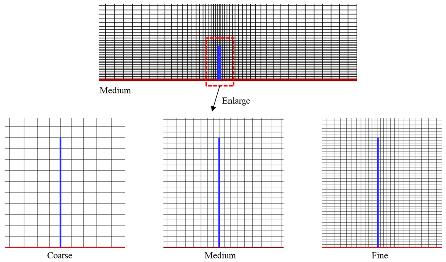
The computational model was constructed using ANSYS ICEM 2024R1. Structured grids were employed in this study due to their high computational stability and quality [63,64]. Given the complexity of the airflow near the construction fence, a high-resolution grid was applied in this region, with a minimum grid size (i.e., the height of the first grid cell near the wall) of 0.1 m at the wall surface. The near-wall mesh was designed to satisfy the requirements of the standard wall function approach, with y⁺ values maintained within the range of 30–300 to ensure the validity of the logarithmic law-of-the-wall treatment. As an example, Figure 3 illustrates the grid layout for the case with a fence height of H_f = 2 m, which was selected based on the results of the grid independence test.

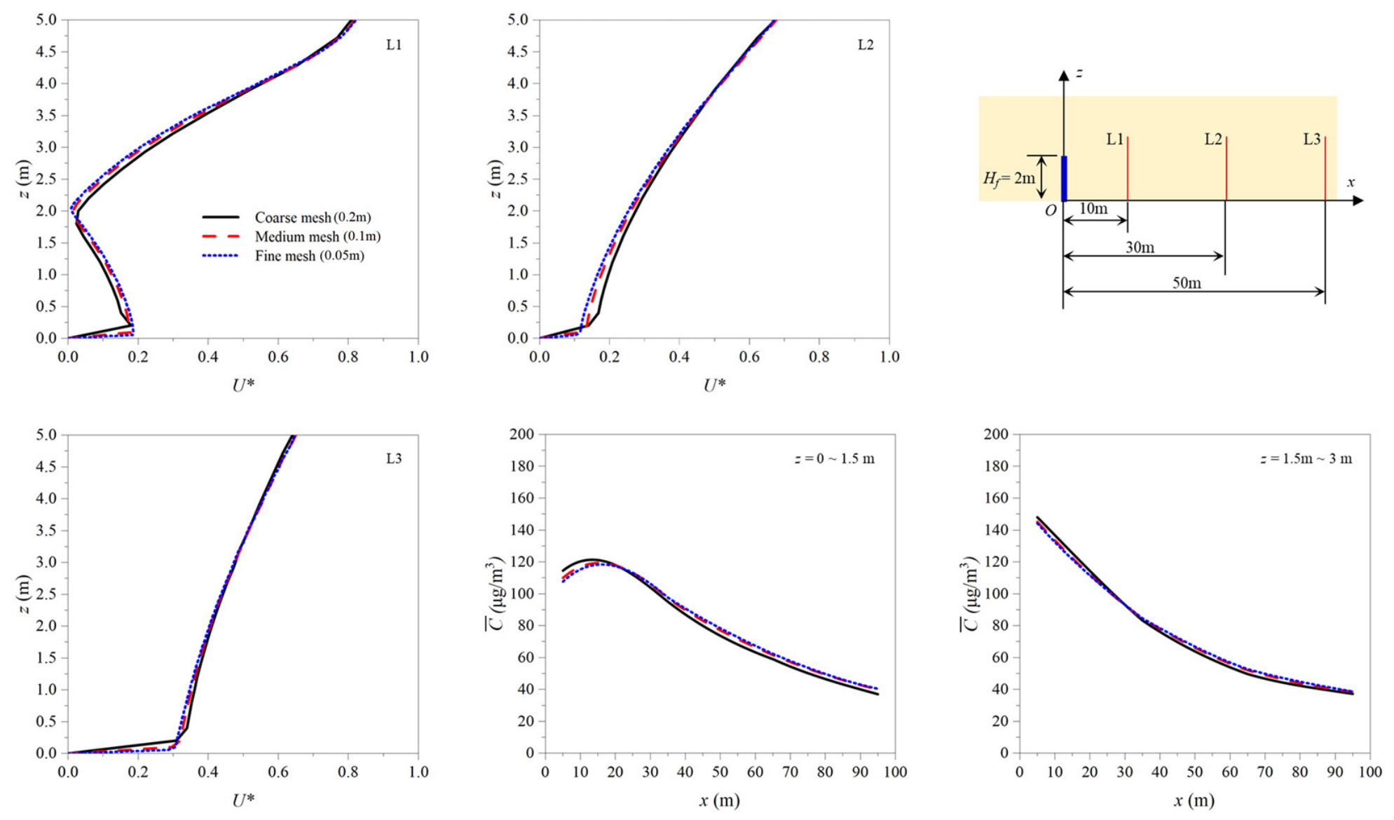
To eliminate the influence of grid resolution on the simulation results, a preliminary simulation was conducted using three different grid systems, namely, coarse, medium, and fine grids, as shown in Figure 3. The minimum grid sizes for these cases were 0.2 m (coarse), 0.1 m (medium), and 0.05 m (fine), with total grid counts of 96,600 (coarse), 374,000 (medium), and 1,224,000 (fine), respectively. To verify the grid independence, the normalized velocity profiles (U* = U/U_ref) at three vertical locations (i.e., L1, L2, and L3) downstream of the fence were analyzed. Moreover, the decay curves of the averaged pollutant concentration ($\overline{C}$, see Equation (18)) between the three grids were also compared for the two regions of z = 0~1.5 m and z = 1.5 m~3 m. The corresponding results are shown in Figure 4.

As illustrated in Figure 4, the profiles of both the velocity and the averaged pollutant concentration obtained from the three grid systems show a consistent trend. However, the results from the medium grid closely match those from the fine grid, whereas the coarse grid shows relatively larger deviations. This indicates that once the grid resolution reaches the medium level, further refinement has minimal impact on the numerical results. To quantify the difference among the three grid resolutions, we further calculated the mean relative error ε using the following formula:

$$\epsilon ={\displaystyle \frac{1}{N}}{\displaystyle \sum _{i=1}^N\left|\frac{{\phi }_i-{\phi }_i^f}{{\phi }_i^f}\right|}\times 100\%$$

(19)

where φ_i represents the results using the coarse or medium mesh. ${\phi }_i^f$ is the results from the fine mesh. N is the total number of sampling points.

Table 3. Mean relative errors between the three meshes.

Parameter	ε
	Coarse vs. Fine	Medium vs. Fine
U*	17.4%	4.9%
$\overline{C}$	5.56%	1.3%

shows the ε between the three mesh resolutions for U* and $\overline{C}$.

It can be found from Table 3 that the ε is 17.4% for U* and 5.56% for $\overline{C}$ between the coarse and fine grids. In contrast, the medium and fine grids yield very similar results, with a mean relative error of only ε = 4.9% for U* and ε = 1.3% for $\overline{C}$, even though the grid number of the fine mesh is 3.3 times that of the medium mesh, suggesting that further mesh refinement beyond the medium level has little impact on simulation accuracy. Therefore, the medium grid was deemed sufficiently accurate for capturing the main flow and mean dispersion patterns, while also being computationally more efficient than the fine mesh.

3. Results and Discussion

3.1. Pressure and Flow Field Distribution Under Different Fence Heights

To visualize the blocking effect of the construction fence on the incoming wind, Figure 5 presents the pressure (P) distribution for the cases with and without the fence. The fence is located at x = 0.

When there is no fence in the domain (i.e., H_f = 0), as shown in Figure 5a, the pressure distribution remains uniform, indicating that the airflow is uninterrupted across the domain. When a low fence (H_f = 1.5 m) is introduced, as shown in Figure 5b, a high-pressure zone appears upstream (x < 0), while a low-pressure region forms downstream (x > 0). This is due to the airflow stagnation at the fence front and the flow recirculation behind it. However, the influence of the fence remains localized, with minimal disruption to the surrounding airflow. For a taller fence (H_f = 3 m), as depicted in Figure 5c, the high-pressure and low-pressure zones expand, leading to a greater pressure gradient across the fence. This suggests that higher fences exert stronger airflow obstruction, further enhancing dust containment.

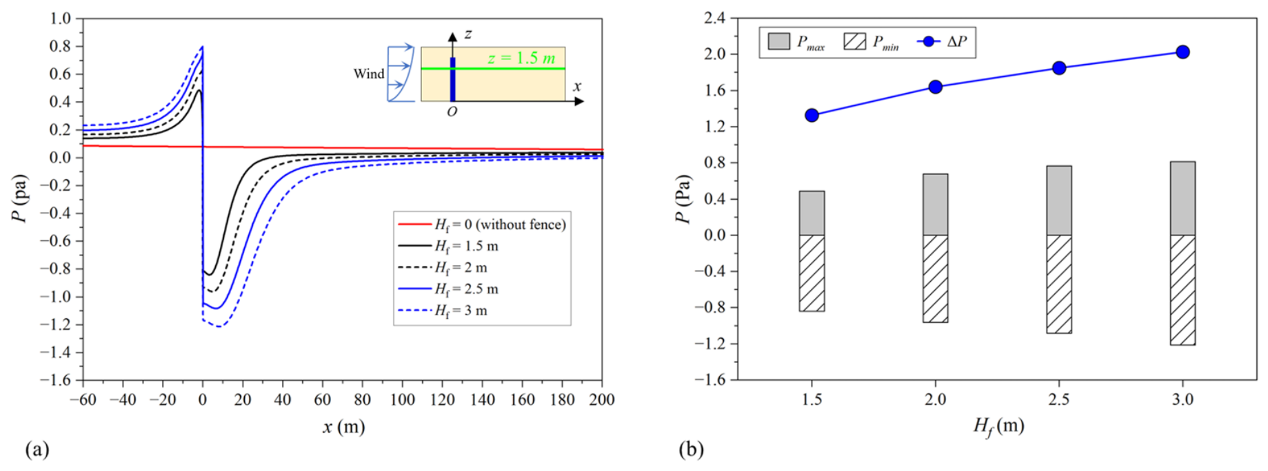
Figure 6 presents the pressure variation along the x-direction at breathing height (z = 1.5 m) for different fence heights (H_f) and the pressure drop (ΔP = P_max − P_min) across the fence. Here, P_max represents the maximum pressure, while P_min denotes the minimum pressure.

As shown in Figure 6a, for the case without the fence (H_f = 0), the pressure profile remains nearly flat, exhibiting only a slight downward trend. However, when a fence is introduced (H_f ≠ 0), the pressure curve rises sharply in the upstream region (x < 0), reaching a peak value P_max. In the downstream region (x > 0), the pressure drops rapidly, reaching a minimum value P_min. As the distance from the fence increases, the pressure gradually recovers to match the background pressure in the no-fence scenario. As illustrated in Figure 6b, an increase in fence height leads to an increase in P_max and a decrease in P_min, thereby amplifying the pressure drop (ΔP) across the fence. Specifically, when H_f is increased from 1.5 m to 3 m, ΔP increases from 1.33 to 2.03, indicating a 53% increase in airflow resistance.

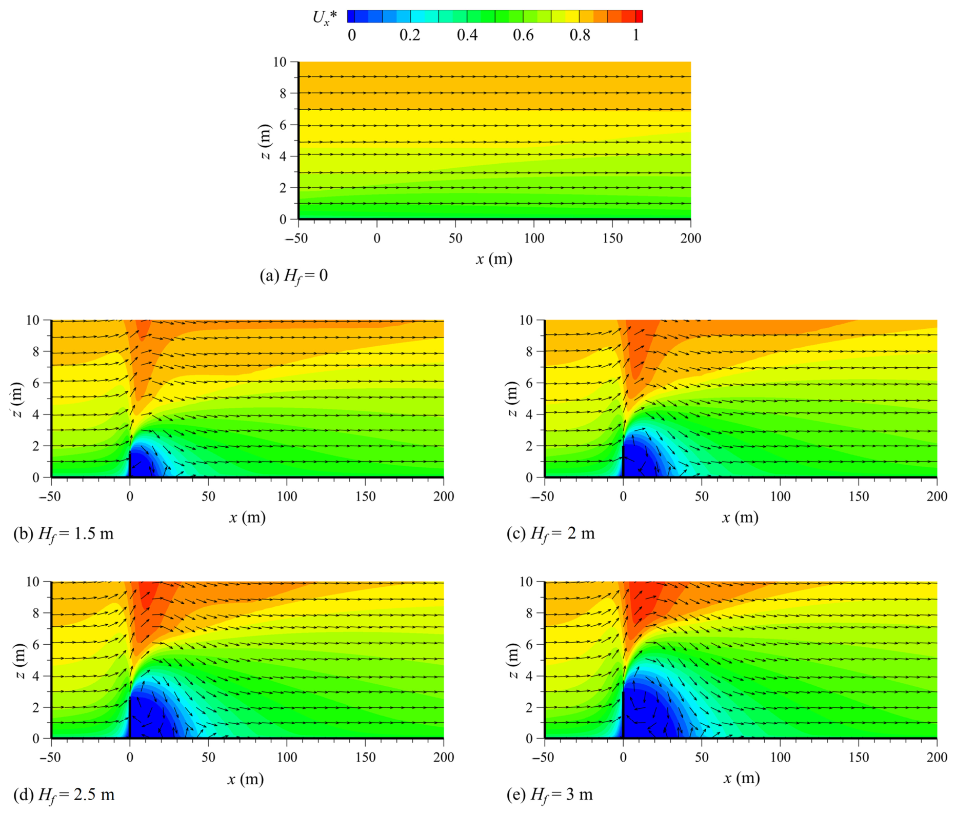
The construction fence significantly affects the trajectory of the background airflow, influencing both the dimensionless horizontal velocity (U_x* = U_x/U_ref) and the dimensionless vertical velocity (U_z* = U_z/U_ref) components. Since U_x* directly affects the transport and dispersion of pollutants from the construction site (x < 0) into the surrounding environment (x > 0), Figure 7 presents the contours of the dimensionless horizontal velocity (U_x*) under different fence heights (H_f).

In the case without the fence (i.e., H_f = 0), as shown in Figure 7a, the flow field within the computational domain closely follows the incoming wind velocity profile, meaning that the flow remains parallel to the ground without any obstructions. Consequently, no significant low-velocity zones or upward air currents are observed. Under these conditions, airflow freely transports pollutants from the construction site (x < 0) into the surrounding environment (x > 0), indicating that background horizontal advection dominates pollutant dispersion.

When the fence is introduced (H_f = 1.5 m) in the domain, as shown in Figure 7b, the background wind is deflected upward due to the blocking effect of the fence. A portion of the airflow surmounts the fence, while a low-velocity recirculation zone develops behind it (x = 0~30 m). Within this recirculation region, U_x* is significantly lower than in surrounding areas, indicating that the fence strongly obstructs horizontal airflow, thereby reducing the efficiency of pollutant dispersion via horizontal advection. After passing through the recirculation region (x > 30 m), the airflow gradually returns to a predominantly horizontal trajectory.

As the fence height is increased from H_f = 1.5 m to 3 m, see Figure 7c–e, the low-velocity recirculation zone expands, extending further downstream and covering a larger vertical range. This implies that higher fences further restrict horizontal airflow, making it more difficult for pollutants to escape via horizontal advection. Overall, within the common range of fence heights (H_f ≤ 3 m), the recirculation region extends approximately 50 m downstream, where horizontal pollutant dispersion is significantly restricted.

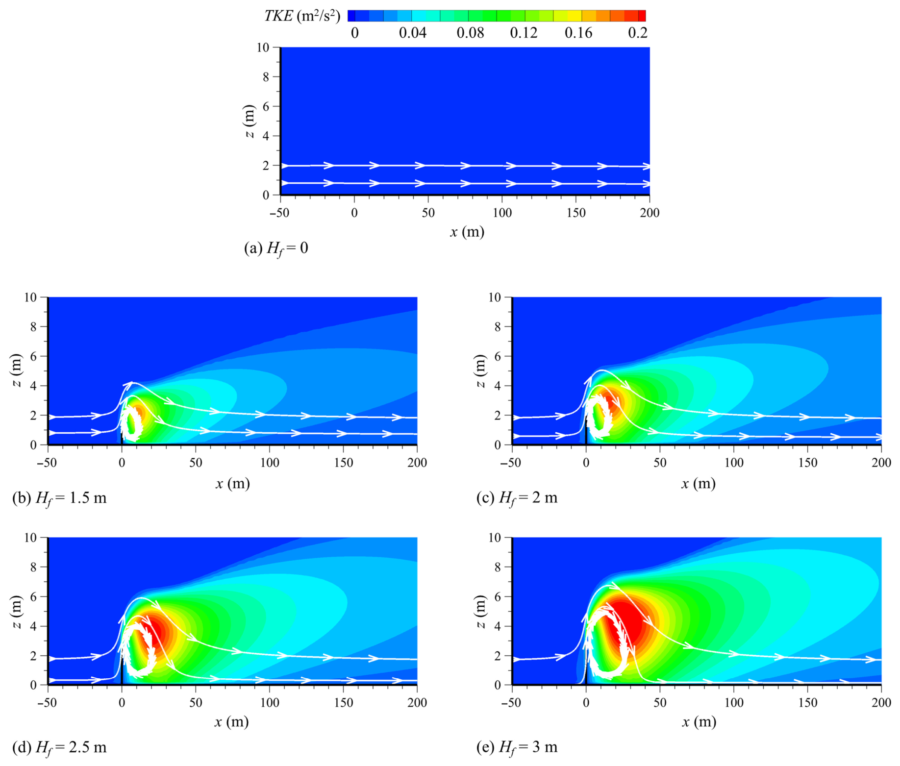
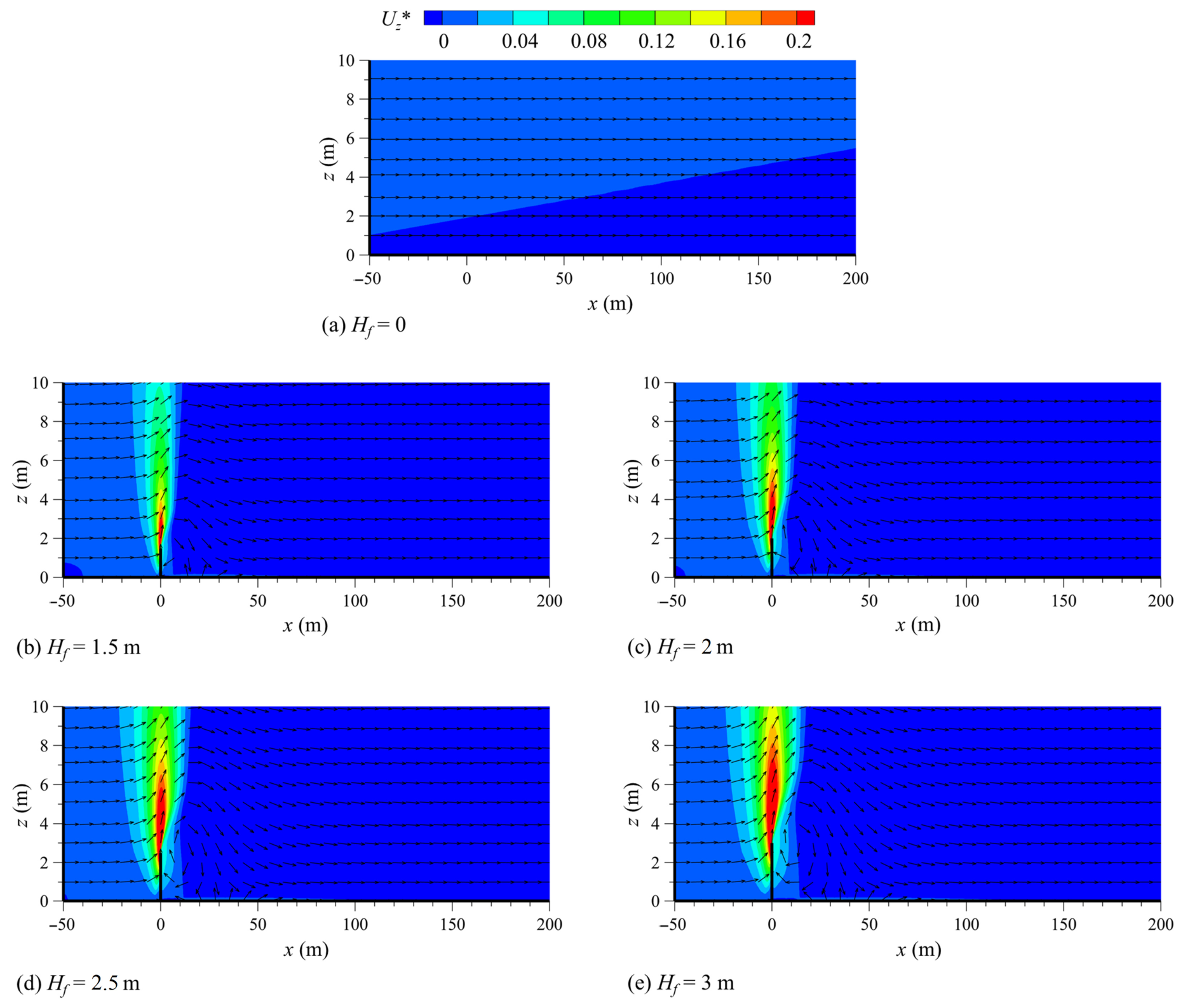
To further illustrate the effects of the fence height on the vertical motion of wind flow, Figure 8 and Figure 9 show the contours of the normalized vertical velocity (U_z*) and the turbulent kinetic energy (TKE) for cases with different fence heights (H_f).

For the case of H_f = 0, as shown in Figure 8a and Figure 9a, the incoming airflow moves horizontally due to the lack of obstruction, resulting in nearly zero vertical velocity (U_z* ≈ 0) and no turbulent generation (TKE ≈ 0). This indicates a highly stable flow regime with minimal vertical movement. When a low fence (H_f = 1.5 m) is introduced in the domain, as shown in Figure 8b and Figure 9b, the fence acts as the barrier that disrupts the incoming flow. Specifically, part of the incoming airflow is forced to rise over the fence, forming a localized vertical upward flow above the fence top, where a significant increase in U_z* is observed. Meanwhile, on the leeward side of the fence, the flow separation occurs, generating a recirculation zone accompanied by enhanced turbulence. This is evidenced by a localized region of elevated TKE behind the fence, representing strong energy input into the turbulence by the fence.

As the fence height increases (see Figure 8c–e and Figure 9c–e), these effects become more pronounced. The upward deflection of the flow intensifies, with stronger and broader vertical airflow movement forming above the fence. Simultaneously, the vortex behind the fence expands, and the associated TKE becomes both larger in magnitude and wider in spatial extent. This indicates that the higher the fence, the more it leads to strong localized disturbances, and these disturbances then promote the vertical flow through enhanced shear and vortex formation at the top and wake of the fence.

From a fluid dynamics perspective, the turbulent kinetic energy generated in the wake region reflects the increased intensity of velocity fluctuations, particularly in the vertical direction. This promotes greater mixing efficiency and enhances the vertical dispersion capacity of the flow. In summary, the fence height modulates the local flow structure in two critical ways: (1) by generating strong vertical upward flow above the fence, and (2) by producing a turbulence-rich wake that supports upward mixing.

3.2. Dust Concentration Distribution Under Different Fence Heights

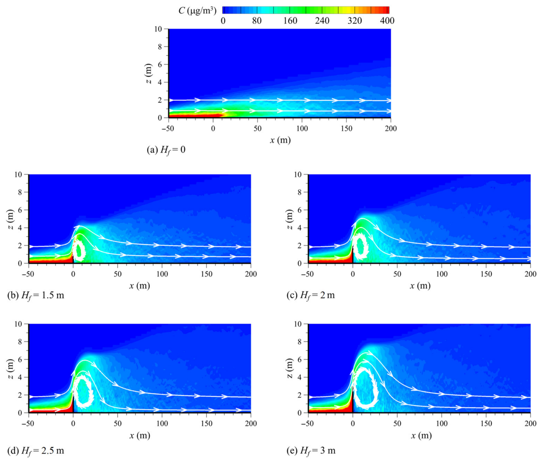
The above results indicate that the presence of a construction fence alters airflow trajectories in both the horizontal and vertical directions, potentially affecting the downstream dispersion and spatial distribution of construction dust. To further investigate the dispersion of pollutants from the construction site into the surrounding environment, Figure 10 presents the contours of pollutant concentration (C) for cases without a fence and with different fence heights (H_f).

As shown in Figure 10a, in the absence of a fence (H_f = 0), pollutants are transported downstream by the horizontal airflow, following the prevailing wind direction. Dust particles emitted from the ground surface of the construction site (x < 0) are directly carried into the external environment (x > 0), resulting in a higher pollutant concentration near the ground, which gradually decreases as the pollutants disperse farther from the site. Within the 100 m downwind region (x = 0~100 m), pollutant concentrations remain relatively high, whereas beyond x > 100 m, concentrations decrease significantly.

When the fence is introduced, as shown in Figure 10b, pollutants within the construction site can no longer disperse freely in the horizontal direction. Instead, vertical airflow induced by the fence redirects some of the pollutants over the top of the fence, allowing them to enter the external environment. Compared to the no-fence case, the pollutant concentration in the external environment is significantly reduced, and the horizontal dispersion range is notably narrowed, with the affected region mainly concentrated within 50 m behind the fence. Beyond x > 50 m, pollutant concentrations decrease substantially, primarily due to the fence’s suppression of horizontal dispersion.

As the fence height (H_f) increases, pollutant concentrations in the external environment decrease further, and the horizontal dispersion range contracts, particularly in near-ground regions where pollutant accumulation is significantly reduced. This is because a taller fence enhances vertical airflow (see Figure 9), forcing pollutants to disperse into higher atmospheric layers, thereby reducing pollutant concentrations in the lower pedestrian breathing zone.

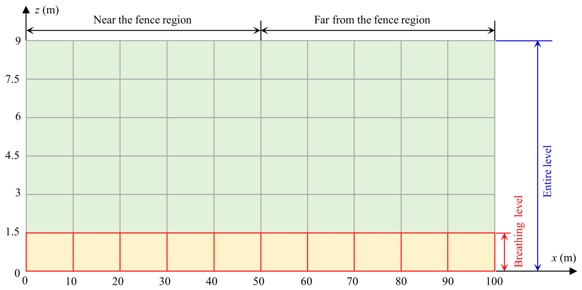
Figure 10 also reveals that due to the blocking effect of the fence, a vortex structure forms behind the fence, leading to the dust concentrations being mostly confined within the region extending up to x < 100 m (especially in x < 50 m) downstream and z < 9 m vertically. As the distance from the dust source increases, the concentration decreases significantly and becomes very low beyond 100 m (i.e., x > 100 m). To better quantify the dispersion process and assess its impact on the surrounding environment, this region (x = 0~100 m, z = 0~9 m) is divided into six uniform vertical layers, as illustrated in Figure 11, each with a height of 1.5 m. The layer below z = 1.5 m is defined as the breathing zone. Additionally, each layer is horizontally divided into ten segments, each 10 m in length, with the average pollutant concentration in each segment calculated as follows:

$$\overline{C}={\displaystyle \underset{A}{\iint }C}dxdz/A$$

(20)

where A represents the area of each segment.

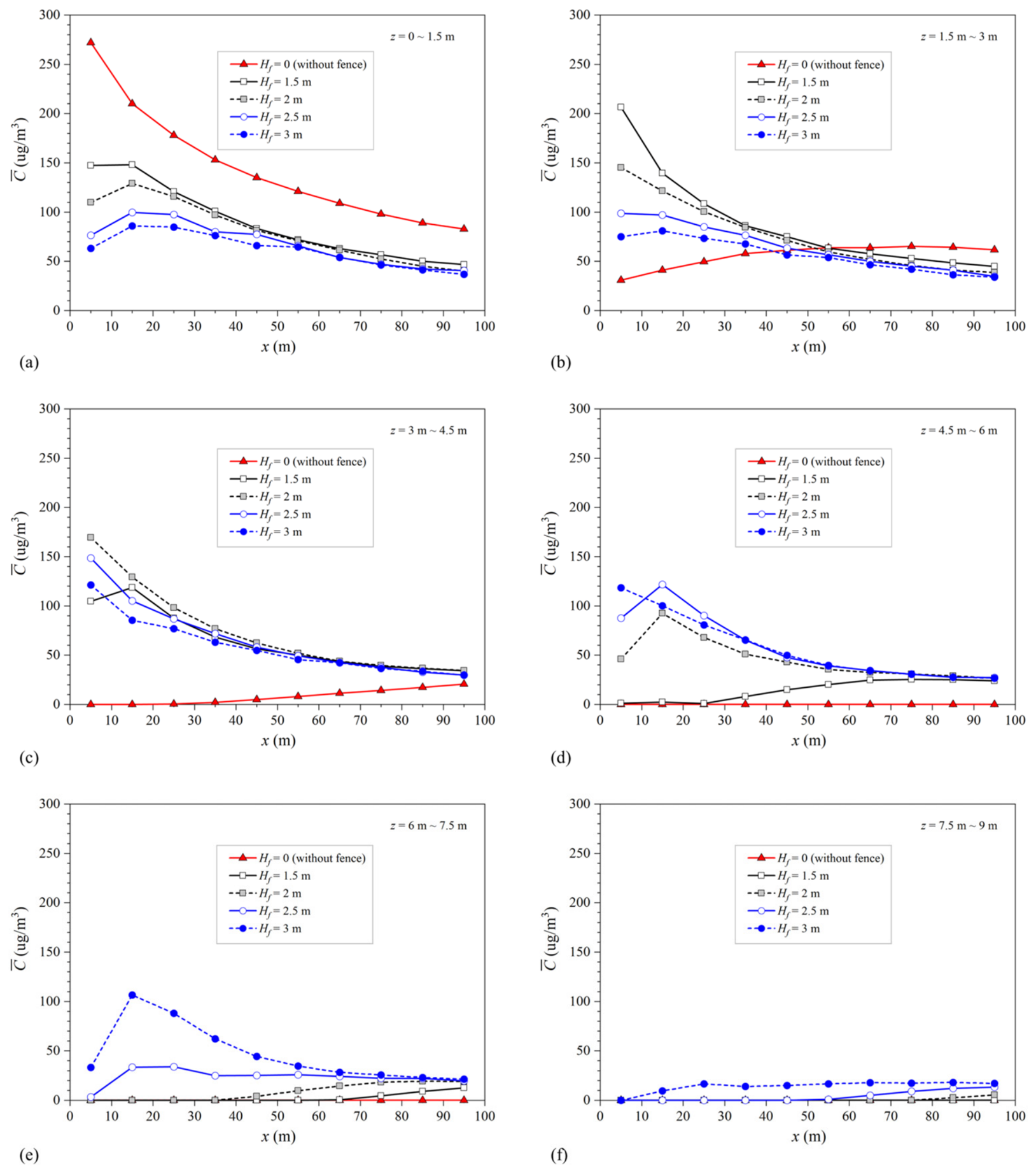
To quantify the horizontal dispersion of pollutants, Figure 12 presents the variation in average pollutant concentration $\overline{C}$ along the x-axis at different vertical heights.

As shown in Figure 12a, for the breathing zone (z = 0~1.5 m) and in the case without fences (H_f = 0), the averaged pollutant concentration $\overline{C}$ decreases monotonically as x increases, indicating continuous horizontal dispersion. However, when a fence is present (H_f = 1.5 m~3 m), $\overline{C}$ profiles are significantly lower than those in the no-fence case, demonstrating that the fence effectively suppresses pollutant escape and mitigates its impact on air quality in the breathing zone. Moreover, due to the formation of a recirculation zone behind the fence, the concentration $\overline{C}$ profile is no longer monotonically decreasing, and a local peak appears at x = 10 m~20 m. This phenomenon suggests that the fence alters airflow patterns, leading to pollutant accumulation in specific areas instead of simple horizontal dispersion.

The results in Figure 12a further indicate that in regions near the fence (x = 0~50 m), particularly x = 0~10 m, the pollutant concentration is highly dependent on fence height: higher fences lead to greater reductions in breathing-zone pollution levels. However, in regions farther from the fence (x > 50 m), the concentration profiles for different fence heights (H_f = 1.5 m~3 m) become nearly identical, suggesting that in these regions, background horizontal airflow dominates dispersion, reducing the fence’s impact.

For higher vertical layers (z > 1.5 m, Figure 12b–f), pollutant concentrations are generally higher in the presence of a fence than in the no-fence case, exhibiting the opposite trend observed in the breathing zone (Figure 12a). In particular, for z > 3 m (Figure 12c–f), pollutant concentrations in the no-fence case are almost zero, indicating that vertical dispersion is limited and pollutants primarily accumulate within the breathing zone. However, when the fence is used at the construction site, the strong vertical airflow lifts pollutants to higher altitudes, thereby reducing ground-level pollution but increasing pollutant accumulation at greater heights. This finding highlights the dual effect of construction fences: they effectively reduce pollution in the breathing zone but simultaneously increase pollutant concentrations at higher elevations.

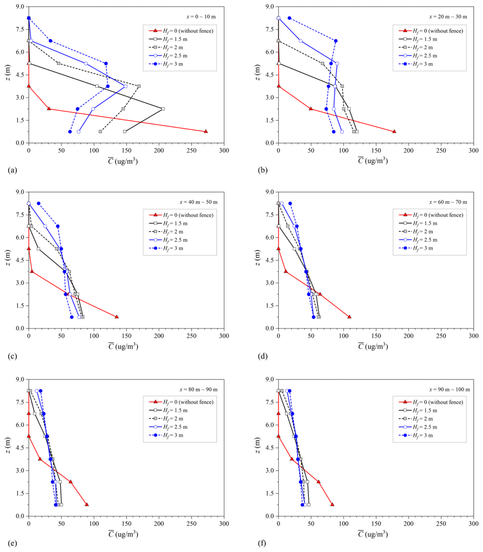
To further analyze the vertical dispersion characteristics, Figure 13 presents the variation in average pollutant concentration $\overline{C}$ with z at different x-locations.

From Figure 13a, it can be observed that for H_f = 0 (without fences), at locations near the construction site (x = 0~10 m), the pollutant concentration decreases monotonically with increasing height (z). The pollutant concentration in the breathing zone (z = 0~1.5 m) is significantly higher than at other heights, and at z > 3 m, the pollutant concentration drops to nearly zero. Moreover, Figure 13a reveals that in the case with the fence, the pollutant concentration exhibits a maximum value at a certain height above the breathing zone. For example, in the case of H_f = 1.5 m, the highest concentration occurs within the z = 1.5 m~3 m height range. Furthermore, with a fence, the average pollutant concentration in the breathing zone is significantly lower than in the no-fence case, whereas the average concentration at higher altitudes is greater than in the absence of a fence. This further demonstrates that the fence effectively reduces pollutant concentration at breathing height but also promotes pollutant accumulation at higher elevations due to enhanced vertical dispersion.

However, as the distance from the construction site increases, particularly at x > 50 m (Figure 13d–f), the pollutant concentration exhibits a monotonically decreasing trend with increasing height (z), regardless of fence presence. Additionally, the concentration in the breathing zone remains consistently higher than at other heights. At greater distances from the construction site (x = 90~100 m), the pollutant concentration profiles for different fence heights (H_f = 1.5 m, 2 m, 2.5 m, and 3 m) become nearly indistinguishable, with minimal variation in pollutant concentration across different heights. As previously noted, this is because the airflow gradually returns to the background horizontal wind pattern, reducing the fence’s influence at greater distances.

3.3. Effectiveness of the Construction Fence

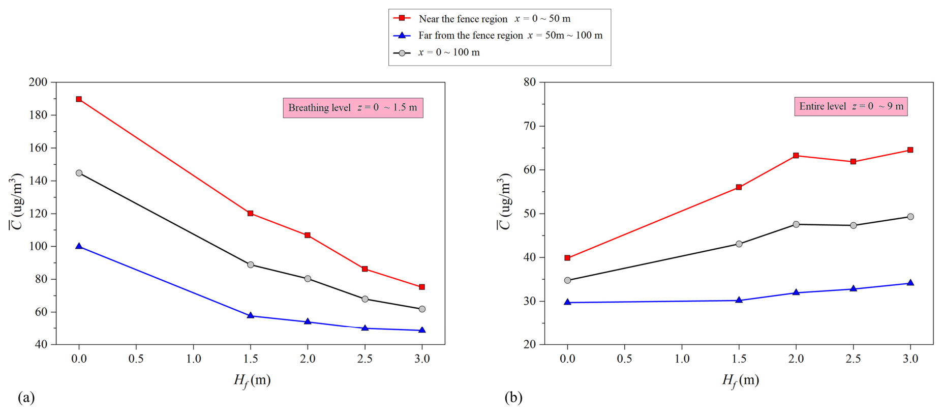
Figure 14 summarizes the variation in average dust concentration ($\overline{C}$) in the surrounding environment with fence height H_f at both breathing height and full height, with the spatial regions defined in Figure 11.

As shown in Figure 14a, within the breathing zone (z = 0~1.5 m), the average pollutant concentration decreases as H_f increases. Furthermore, the reduction in pollutant concentration is more pronounced in the area close to the fence (x = 0~50 m) compared to the region (x = 50~100 m) farther away. Overall, these results indicate that the fence effectively mitigates the impact of construction dust on ambient air quality at breathing height.

However, when considering the entire height range (z = 0~9 m), as illustrated in Figure 14b, the average pollutant concentration increases with H_f, displaying an opposite trend to that observed in the breathing zone. This suggests that the pollutant concentration above breathing height increases as H_f increases. The likely explanation is that the presence of the fence enhances vertical air movement, facilitating the upward transport of pollutants into higher atmospheric layers. This finding further highlights the dual effect of fences on surrounding air quality: while they reduce pollutant concentration in the breathing zone, they simultaneously promote pollutant accumulation at higher elevations.

Since human exposure is primarily associated with air quality at the breathing height, the construction fence can be considered effective in reducing the adverse impact of construction dust on the surrounding public space. Nevertheless, the increase in upper-level pollution may pose potential concerns, especially for buildings located close to construction sites. For example, in situations where natural ventilation is achieved through open windows in upper floors, there is a risk of dust intrusion. Therefore, the fence design and construction management should not only focus on ground-level dust control, but also consider that rising dust could affect nearby buildings by reaching their facades or entering upper-floor rooms through open windows.

To further quantify the impact of the fence on pollutant concentration, the pollutant removal percentage (σ_C) is defined as:

$${\sigma }_C={\displaystyle \frac{\overline{C_0}-\overline{C_i}}{\overline{C_0}}}\times 100\%$$

(21)

where $\overline{C_i}$ and $\overline{C_0}$ represent the average pollutant concentrations with and without fences, respectively. When σ_C > 0, the fence reduces pollutant concentration in the external environment, whereas σ_C < 0 indicates that the fence aggravates pollutant accumulation.

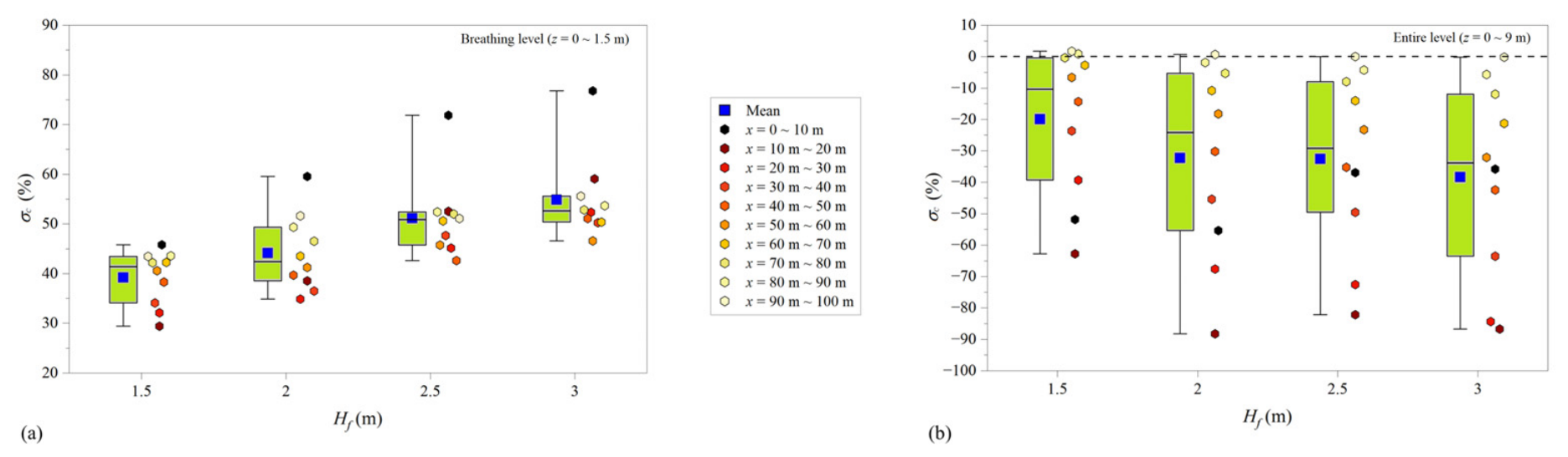
According to Equation (19), Figure 15 presents the variation in σ_C with H_f.

As illustrated in Figure 15a, within the breathing zone, σ_C increases with H_f. Specifically, as H_f increases, the amount of pollutants escaping from the construction site into the breathing zone decreases, thereby improving air quality for pedestrians. The mean pollutant reduction percentages for different fence heights (H_f = 1.5 m, 2 m, 2.5 m, and 3 m) are approximately σ_C = 39%, 44%, 51%, 55%, respectively. In areas near the fence (x = 0~10 m, black symbols in Figure 15a), the pollutant removal effect is most significant, reaching σ_C = 76% for H_f = 3 m. However, for the entire height range (z = 0~9 m), as shown in Figure 15b, σ_C < 0, indicating that the fence increases overall pollutant concentration compared to the no-fence case. Furthermore, for H_f = 1.5 m, 2 m, 2.5 m, and 3 m, the mean σ_C values are −20%, −32.2%, −32.6%, and −38.4%, respectively. This suggests that for H_f = 2 m~3 m, the increase in pollutant accumulation at higher altitudes becomes more pronounced, but the change in σ_C is not highly significant.

3.4. Discussion

3.4.1. Recommendations for Optimizing Fence Design

The findings of this study indicate that construction fences can effectively reduce dust exposure within the pedestrian breathing zone; however, they may also induce pollutant accumulation at higher elevations due to enhanced flow blockage, shear-layer formation, and upward transport induced by flow separation. This dual effect highlights the importance of understanding the aerodynamic mechanisms governing both near-ground protection and vertical pollutant redistribution.

In the present study, only solid impermeable fences were investigated. The results demonstrate that strong flow separation at the fence crest and the resulting shear-layer development are the primary drivers of upward pollutant transport and elevated concentration zones above the fence height. These mechanisms provide a physical basis for considering potential design improvements.

Based on these identified flow characteristics and supported by previous studies on windbreak aerodynamics, several mechanism-informed optimization directions can be suggested. For example, partially permeable fence structures or designs that introduce controlled flow leakage near the upper section may help reduce pressure differences and weaken shear-layer intensity. Similarly, aerodynamic modifications of the fence top geometry, such as rounded or inclined edges, may mitigate flow separation strength and reduce vertical pollutant transport.

It should be emphasized that these suggestions are not directly validated in the present simulations, but are proposed as qualitative design implications derived from the observed flow mechanisms. A multi-objective design framework considering both near-ground exposure reduction and overall pollutant dispersion control may provide a more balanced strategy for urban construction fence optimization.

3.4.2. Limitations and Future Work

Although the present study has been validated against field measurements and is able to reproduce the main trends of dust concentration decay, several limitations should be acknowledged and may be addressed in future research to enhance the robustness and applicability of the findings.

First, a two-dimensional (2D) modeling framework was adopted to represent the vertical central plane of the construction site; however, this simplification neglects spanwise variations and three-dimensional (3D) end effects near fence terminals. As a result, the model may slightly overestimate the downstream extent of wake recirculation due to the absence of lateral entrainment and 3D momentum exchange. Nevertheless, this limitation is expected to have limited influence on the main conclusions of this study, since the analysis focuses on the central region of long, continuously arranged fences where lateral flow non-uniformity is weak and the flow can be reasonably approximated as quasi-two-dimensional. Under these conditions, the conclusions are applicable to construction sites with sufficiently long and continuous fences and dominant wind directions approximately perpendicular to the fence alignment.

Second, a limitation of this study is that only a single representative wind speed (U_ref = 2.2 m/s) was considered in the numerical simulations. While this approach enables a controlled comparison of different fence configurations under a consistent background flow, it does not explicitly account for the variability of wind speed under different meteorological conditions. It should be noted that variations in wind speed may influence the absolute magnitude of airflow velocity and pollutant concentration. Therefore, the key qualitative conclusions are expected to remain valid within a reasonable range of wind speed conditions. Future work should incorporate a systematic wind-speed sensitivity analysis to further quantify the robustness of the findings under varying meteorological scenarios.

On the other hand, the secondary resuspension of deposited particles was not considered. Particles impacting the ground or fence surfaces were assumed to be permanently captured, and re-entrainment under turbulent shear was not modeled. This simplification may lead to an underestimation of absolute downstream dust concentrations, particularly in high-turbulence wake regions near the fence. However, since this assumption is applied consistently across all cases, the relative comparison of different fence configurations is not expected to be significantly affected, and the main conclusions remain qualitatively robust. Future work should consider resuspension effects to improve prediction accuracy.

Finally, the analysis focused on a single particle size and did not consider the effect of particle size distribution. In reality, particles of different sizes exhibit diverse dispersion behaviors due to their varying settling velocities and inertial properties. Future studies should consider multiple particle classes to provide a more comprehensive assessment of pollution transport and exposure risk, particularly at breathing height.

Despite these limitations, the study makes a substantial contribution by systematically revealing how fence height alters local flow structures and affects vertical pollutant transport, supported by experimental validation. Addressing the above issues in future research would further strengthen the robustness and applicability of the findings.

4. Summary and Conclusions

Construction dust poses severe air pollution challenges to the surrounding environment. While construction fences are commonly adopted to limit dust dispersion, their actual effectiveness and influence on pollutant transport patterns remain inadequately understood, because the existing research relying on field measurements or empirical models was constrained by monitoring site distribution and spatial resolution. Thus, there is a lack of systematic quantification of the dust suppression performance of fences. In this study, a reliable CFD numerical simulation approach was developed to examine the spatial distribution of construction dust and quantify the dust suppression efficiency of fences at different heights.

Three widely used turbulence models, i.e., the Standard, RNG, and Realizable k-ε models, were tested using field measurement data for validation. All three models reproduced the dust concentration decay trend with reasonable accuracy, while the RNG k-ε model achieved the best agreement (q = 1, FB = 0.052, NMSE = 0.028), outperforming the other two models. These results confirm the feasibility and reliability of the proposed simulation framework.

Moreover, it was found that construction fences can effectively reduce dust dispersion into the surrounding environments, particularly within the breathing zone (z = 0~1.5 m). For example, when the fence height (H_f) is increased from 1.5 m to 3 m, the dust concentration in the breathing zone decreases significantly, and the reduction rate increases from 39% to 55%. This shows the important role of construction fences in improving urban air quality at the pedestrian level.

However, it should be noted that fences also exhibit adverse side effects. For the entire height range (z = 0~9 m), the dust concentration increases in the case with the fence compared to the no-fence case, and higher fences exacerbate this adverse effect, with the overall dust concentration increasing by approximately 20% to 38% compared to the no-fence case. This highlights the dual impacts of the fences on surrounding air quality, i.e., while the fences reduce pollutant concentrations in the breathing zone, they also result in pollutant accumulation at higher altitudes. Thus, to provide a more comprehensive basis for optimizing construction dust control strategies, the fence height should be selected based on a balance between near-ground exposure reduction and upper-level dispersion effects. In particular, the upward transport of pollutants may increase the likelihood of exposure at higher elevations in surrounding buildings, such as through windows or natural ventilation openings, which should be considered in practical construction site management rather than simply increasing fence height.

References

1. Apte, J.S.; Brauer, M.; Cohen, A.J.; Ezzati, M.; Pope, C.A., III. Ambient PM2.5 reduces global and regional life expectancy. Environ. Sci. Technol. Lett. 2018, 5, 546–551. [Google Scholar] [CrossRef]
2. Ma, G.; Wang, J.; Yu, F.; Guo, X.; Zhang, Y.; Li, C. Assessing the premature death due to ambient particulate matter in China’s urban areas from 2004 to 2013. Front. Environ. Sci. Eng. 2016, 10, 7. [Google Scholar] [CrossRef]
3. Paschalidou, A.; Kassomenos, P.; Kelessis, A. Tracking the association between metro-railway construction works and PM levels in an urban Mediterranean environment. Sci. Total Environ. 2016, 568, 1326–1332. [Google Scholar] [CrossRef] [PubMed]
4. Tao, G.; Feng, J.; Feng, H.; Feng, H.; Zhang, K. Reducing construction dust pollution by planning construction site layout. Buildings 2022, 12, 531. [Google Scholar] [CrossRef]
5. Yan, H.; Li, Q.; Feng, K.; Zhang, L. The characteristics of PM emissions from construction sites during the earthwork and foundation stages: An empirical study evidence. Environ. Sci. Pollut. Res. 2023, 30, 62716–62732. [Google Scholar] [CrossRef]
6. Giunta, M. Sustainable Practices in Road Constructions: Estimation and Mitigation of Impact on Air Quality. Transp. Res. Procedia 2023, 69, 139–146. [Google Scholar] [CrossRef]
7. Qiu, X.; Duan, L.; Gao, J.; Wang, S.; Chai, F.; Hu, J.; Zhang, J.; Yun, Y. Chemical composition and source apportionment of PM10 and PM2.5 in different functional areas of Lanzhou, China. J. Environ. Sci. 2016, 40, 75–83. [Google Scholar] [CrossRef]
8. Van Pelt, R.S.; Zobeck, T.M. Chemical constituents of fugitive dust. Environ. Monit. Assess. 2007, 130, 3–16. [Google Scholar] [CrossRef] [PubMed]
9. National Bureau of Statistics of China. 2024. Available online: https://www.stats.gov.cn/sj/zxfb/202601/t20260119_1962324.html (accessed on 20 February 2026).
10. World Health Organization. WHO Global Air Quality Guidelines: Particulate Matter (PM2.5 and PM10), Ozone, Nitrogen Dioxide, Sulfur Dioxide and Carbon Monoxide; WHO: Geneva, Switzerland, 2021.
11. Kebe, M.; Traore, A.; Sow, M.; Fall, S.; Tahri, M. Human health risk evaluation of particle air pollution (PM10 and PM2.5) and heavy metals in Dakar’s two urban areas. Asian J. Atmos. Environ. 2025, 19, 7. [Google Scholar] [CrossRef]
12. Keer, S.; Brooks, C.; Glass, B.; McLean, D.; Harding, E.; Douwes, J. Respiratory symptoms and use of dust-control measures in New Zealand construction workers–A cross-sectional study. PLoS ONE 2022, 17, e0266668. [Google Scholar] [CrossRef] [PubMed]
13. Azarmi, F.; Kumar, P.; Marsh, D.; Fuller, G. Assessment of the long-term impacts of PM 10 and PM 2.5 particles from construction works on surrounding areas. Environ. Sci. Process. Impacts 2016, 18, 208–221. [Google Scholar] [CrossRef] [PubMed]
14. Kim, H.; Lai, K.; Cisse, T.; Wei, X.; Ge, E. Association between air pollution and chronic cough: Evidence from a systematic review and meta-analysis of observational studies. Environ. Res. 2026, 297, 124108. [Google Scholar] [CrossRef] [PubMed]
15. Maqsood, R.; Nisar, N. Spirometry Analysis of Respiratory Issues in Construction Industry Workers of Shakargarh and Lahore. Int. J. Adv. Sustain. Dev. (IJASD) 2025, 2, 40–49. [Google Scholar] [CrossRef]
16. Gangolells, M.; Casals, M.; Gassó, S.; Forcada, N.; Roca, X.; Fuertes, A. A methodology for predicting the severity of environmental impacts related to the construction process of residential buildings. Build. Environ. 2009, 44, 558–571. [Google Scholar] [CrossRef]
17. Zheng, L.; Feng, Z.; Liu, J.; Han, L.; Wang, H. Cross-concentration calibration of low-cost sensors for effective dust monitoring at construction sites. J. Aerosol Sci. 2024, 182, 106456. [Google Scholar] [CrossRef]
18. Tian, G.; Li, G.; Yan, B.-L.; Huang, Y.-H.; Qin, J.-P. Spatial dispersion laws of fugitive dust from construction sites. Environ. Sci. 2008, 29, 259–262. [Google Scholar]
19. Manzhilevskaya, S. Dust pollution in construction sites in point-pattern housing development. Buildings 2024, 14, 2991. [Google Scholar] [CrossRef]
20. Yi, M.; Fu, Y.; Liu, J. Calculation of carbon emissions during construction using the carbon emission factor method. In Proceedings of the 28th International Symposium on Advancement of Construction Management and Real Estate; Springer: Singapore, 2023; pp. 1137–1148. [Google Scholar]
21. Zhang, G.; Sandanayake, M.; Setunge, S.; Li, C.; Fang, J. Selection of emission factor standards for estimating emissions from diesel construction equipment in building construction in the Australian context. J. Environ. Manag. 2017, 187, 527–536. [Google Scholar] [CrossRef]
22. Liu, W.; Tang, P.; Li, K.; Jiang, T. Demolition dust formation, diffusion mechanism and monitoring quantitative research on demolition of existing buildings. Appl. Ecol. Environ. Res. 2019, 17, 14543–14559. [Google Scholar] [CrossRef]
23. Muleski, G.E.; Cowherd, C., Jr.; Kinsey, J.S. Particulate emissions from construction activities. J. Air Waste Manag. Assoc. 2005, 55, 772–783. [Google Scholar] [CrossRef] [PubMed]
24. Hang, J.; Liang, J.; Wang, X.; Zhang, X.; Wu, L.; Shao, M. Investigation of O3–NOx–VOCs chemistry and pollutant dispersion in street canyons with various aspect ratios by CFD simulations. Build. Environ. 2022, 226, 109667. [Google Scholar] [CrossRef]
25. Yim, S.H.L.; Fung, J.C.H.; Lau, A.K.H.; Kot, S.C. Air ventilation impacts of the “wall effect” resulting from the alignment of high-rise buildings. Atmos. Environ. 2009, 43, 4982–4994. [Google Scholar] [CrossRef]
26. Yuan, C.; Ng, E.; Norford, L.K. Improving air quality in high-density cities by understanding the relationship between air pollutant dispersion and urban morphologies. Build. Environ. 2014, 71, 245–258. [Google Scholar] [CrossRef] [PubMed]
27. Dyck, R.I.J.; Stukel, J.J. Fugitive dust emissions from trucks on unpaved roads. Environ. Sci. Technol. 1976, 10, 1046–1048. [Google Scholar] [CrossRef]
28. Wang, H.; Cheng, W.; Sun, B.; Ma, Y. Effects of radial air flow quantity and location of an air curtain generator on dust pollution control at fully mechanized working face. Adv. Powder Technol. 2017, 28, 1780–1791. [Google Scholar] [CrossRef]
29. Cai, P.; Nie, W.; Chen, D.; Yang, S.; Liu, Z. Effect of air flowrate on pollutant dispersion pattern of coal dust particles at fully mechanized mining face based on numerical simulation. Fuel 2019, 239, 623–635. [Google Scholar] [CrossRef]
30. Çoşkun, Ş.; Hazaveh, H.A.; Uzol, O.; Kurç, Ö. Experimental investigation of wake flow field and wind comfort characteristics of fractal wind fences. J. Wind Eng. Ind. Aerodyn. 2017, 168, 32–47. [Google Scholar] [CrossRef]
31. Mahgoub, A.O.; Ghani, S. Numerical and experimental investigation of utilizing the porous media model for windbreaks CFD simulation. Sustain. Cities Soc. 2021, 65, 102648. [Google Scholar] [CrossRef]
32. Raine, J.K.; Stevenson, D.C. Wind protection by model fences in a simulated atmospheric boundary layer. J. Wind Eng. Ind. Aerodyn. 1977, 2, 159–180. [Google Scholar] [CrossRef]
33. Kim, R.-W.; Lee, I.-B.; Kwon, K.-S.; Yeo, U.-H.; Lee, S.-Y.; Lee, M.-H. Design of a windbreak fence to reduce fugitive dust in open areas. Comput. Electron. Agric. 2018, 149, 150–165. [Google Scholar] [CrossRef]
34. Shyy, W. Computational Fluid Dynamics with Moving Boundaries; CRC Press: Boca Raton, FL, USA, 1995. [Google Scholar]
35. Franke, J. Recommendations of the COST action C14 on the use of CFD in predicting pedestrian wind environment. In Proceedings of the 4th International Symposium on Computational Wind Engineering, Yokohama, Japan, 16–19 July 2006; pp. 529–532. [Google Scholar]
36. Tominaga, Y.; Mochida, A.; Yoshie, R.; Kataoka, H.; Nozu, T.; Yoshikawa, M.; Shirasawa, T. AIJ guidelines for practical applications of CFD to pedestrian wind environment around buildings. J. Wind Eng. Ind. Aerodyn. 2008, 96, 1749–1761. [Google Scholar] [CrossRef]
37. JGJ/T 338–2014; Standard for Wind Tunnel Test of Buildings and Structures. China Architecture & Building Press: Beijing, China, 2014.
38. Wang, Y.; Qi, M.; Lu, Y. Integrated impacts of surrounding building density and gap permeability on pollutant dispersion in four-way street networks. Sci. Total Environ. 2024, 957, 177440. [Google Scholar] [CrossRef] [PubMed]
39. Yang, F.; Kang, Y.; Gao, Y.; Zhong, K. Numerical simulations of the effect of outdoor pollutants on indoor air quality of buildings next to a street canyon. Build. Environ. 2015, 87, 10–22. [Google Scholar] [CrossRef]
40. China Meteorological Administration. Haidian District, Beijing, Station No. 54511. Available online: https://data.cma.cn/ (accessed on 20 February 2026).
41. Barth, T.; Jespersen, D. The design and application of upwind schemes on unstructured meshes. In Proceedings of the 27th Aerospace Sciences Meeting, Reno, NV, USA, 9–12 January 1989; p. 366. [Google Scholar]
42. Buccolieri, R.; Sandberg, M.; Di Sabatino, S. City breathability and its link to pollutant concentration distribution within urban-like geometries. Atmos. Environ. 2010, 44, 1894–1903. [Google Scholar] [CrossRef]
43. Serra, N.; Semiao, V. ESIMPLE, a new pressure–velocity coupling algorithm for built-environment CFD simulations. Build. Environ. 2021, 204, 108170. [Google Scholar] [CrossRef]
44. Fluent, A. Ansys Fluent Theory Guide; Ansys Inc.: Canonsburg, PA, USA, 2011; Volume 15317, pp. 724–746. [Google Scholar]
45. Kurnia, J.C.; Sasmito, A.P.; Hassani, F.P.; Mujumdar, A.S. Introduction and evaluation of a novel hybrid brattice for improved dust control in underground mining faces: A computational study. Int. J. Min. Sci. Technol. 2015, 25, 537–543. [Google Scholar] [CrossRef]
46. Xu, C.; Nie, W.; Peng, H.; Zhang, S.; Liu, F.; Yi, S.; Cha, X.; Mwabaima, F.I. Numerical simulation of the dynamic wetting of coal dust by spray droplets. Energy 2023, 270, 126667. [Google Scholar] [CrossRef]
47. Chan, A.T.; So, E.S.; Samad, S.C. Strategic guidelines for street canyon geometry to achieve sustainable street air quality. Atmos. Environ. 2001, 35, 4089–4098. [Google Scholar] [CrossRef]
48. Huang, H.; Akutsu, Y.; Arai, M.; Tamura, M. A two-dimensional air quality model in an urban street canyon: Evaluation and sensitivity analysis. Atmos. Environ. 2000, 34, 689–698. [Google Scholar] [CrossRef]
49. Yakhot, V.; Orszag, S.A. Renormalization group analysis of turbulence. I. Basic theory. J. Sci. Comput. 1986, 1, 3–51. [Google Scholar] [CrossRef]
50. Liu, G.; Guo, X.; Cheng, W.; Chen, L.; Cui, X. Investigating the migration law of aggregates during concrete flowing in pipe. Constr. Build. Mater. 2020, 251, 119065. [Google Scholar] [CrossRef]
51. Zhou, F.; Hu, S.; Liu, Y.; Liu, C.; Xia, T. CFD–DEM simulation of the pneumatic conveying of fine particles through a horizontal slit. Particuology 2014, 16, 196–205. [Google Scholar] [CrossRef]
52. Yang, X.; Yu, H.; Wang, Y.; Cheng, W. Investigation of dust pollution control rules in tunnel excavation based on modularized airflow diverging system. Build. Environ. 2022, 221, 109356. [Google Scholar] [CrossRef]
53. Zhang, F.; Lu, Y.; Wang, Y.; Jiang, Z.; Liu, J.; Chen, J. Study on dust pollution law and chemical dust suppression technology of non hard pavement in urban construction sites. Build. Environ. 2023, 229, 109938. [Google Scholar] [CrossRef]
54. Corson, D.; Jaiman, R.; Shakib, F. Industrial application of RANS modelling: Capabilities and needs. Int. J. Comput. Fluid Dyn. 2009, 23, 337–347. [Google Scholar] [CrossRef]
55. Hami, K. Turbulence Modeling a Review for Different Used Methods. Int. J. Heat Technol. 2021, 39, 227–234. [Google Scholar] [CrossRef]
56. Serra, N. Revisiting RANS turbulence modelling used in built-environment CFD simulations. Build. Environ. 2023, 237, 110333. [Google Scholar] [CrossRef]
57. Orszag, S.A.; Staroselsky, I.; Flannery, W.; Zhang, Y. Introduction to renormalization group modeling of turbulence. In Simulation and Modelling of Turbulent Flows; Oxford University Press: Oxford, UK, 1996; pp. 155–183. [Google Scholar]
58. Park, I.H.; Cho, Y.J.; Lee, J.S. Analysis of Empirical Constant of Eddy Viscosity by k-ε and RNG k-ε Turbulence Model in Wake Simulation. J. Korean Soc. Mar. Environ. Saf. 2019, 25, 344–353. [Google Scholar] [CrossRef]
59. Hurnik, M.; Ciuman, P.; Popiolek, Z. Eddy–viscosity Reynolds-averaged Navier–Stokes modeling of air distribution in a sidewall jet supplied into a room. Energies 2024, 17, 1261. [Google Scholar] [CrossRef]
60. Du, Y.; Blocken, B.; Pirker, S. A novel approach to simulate pollutant dispersion in the built environment: Transport-based recurrence CFD. Build. Environ. 2020, 170, 106604. [Google Scholar] [CrossRef]
61. Hanna, S.R.; Hansen, O.R.; Dharmavaram, S. FLACS CFD air quality model performance evaluation with Kit Fox, MUST, Prairie Grass, and EMU observations. Atmos. Environ. 2004, 38, 4675–4687. [Google Scholar] [CrossRef]
62. Tominaga, Y.; Stathopoulos, T. CFD simulations of near-field pollutant dispersion with different plume buoyancies. Build. Environ. 2018, 131, 128–139. [Google Scholar] [CrossRef]
63. Hefny, M.M.; Ooka, R. CFD analysis of pollutant dispersion around buildings: Effect of cell geometry. Build. Environ. 2009, 44, 1699–1706. [Google Scholar] [CrossRef]
64. Palusci, O.; Monti, P.; Cecere, C.; Montazeri, H.; Blocken, B. Impact of morphological parameters on urban ventilation in compact cities: The case of the Tuscolano-Don Bosco district in Rome. Sci. Total Environ. 2022, 807, 150490. [Google Scholar] [CrossRef] [PubMed]
Figure 1. Simplified two-dimensional model of the construction site and boundary conditions.
Sustainability 18 07432 g001
Figure 2. Comparisons of the simulated results from the three turbulence models and measured data. The circles represent the measured data points, and the black line represents the fitted curve of the measured data; the red, blue, and green curves represent the numerical results of the RNG k-ε, Standard k-ε, and Realizable k-ε models, respectively.
Sustainability 18 07432 g002
Figure 3. Grid layouts for coarse, medium, and fine meshes. The minimum grid sizes are 0.2 m (coarse), 0.1 m (medium), and 0.05 m (fine), with corresponding total cell numbers of 96,600, 374,000, and 1,224,000, respectively.
Sustainability 18 07432 g003
Figure 4. Comparison of the velocity (U*) and concentration ( C ¯ ) between the coarse, medium, and fine meshes at different vertical lines (L1, L2 and L3). The horizontal coordinate x denotes the horizontal distance from the fence, z is the vertical distance from the ground (z = 0).
Sustainability 18 07432 g004
Figure 5. Pressure (P) contours overlaid with wind velocity vectors (arrows indicate wind flow direction) for different dust control fence heights: (a) Hf = 0, (b) Hf = 1.5 m and (c) Hf = 3 m.
Sustainability 18 07432 g005
Figure 6. Pressure distribution characteristics around the fence. (a) Pressure P variation along the x-direction at breathing height (z = 1.5 m) for different fence heights (Hf), and (b) the corresponding pressure drop (ΔP = PmaxPmin) across the fence. Here, Pmax represents the maximum pressure, while Pmin denotes the minimum pressure.
Sustainability 18 07432 g006
Figure 7. Contours of the dimensionless horizontal velocity (Ux*), overlaid with black velocity vectors (arrow orientation denotes local airflow direction): (a) Hf = 0, (b) Hf = 1.5 m, (c) Hf = 2 m, (d) Hf = 2.5 m, (e) Hf = 3 m.
Sustainability 18 07432 g007
Figure 8. Contours of normalized vertical velocity (Uz*), overlaid with black velocity vectors: (a) Hf = 0, (b) Hf = 1.5 m, (c) Hf = 2 m, (d) Hf = 2.5 m, (e) Hf = 3 m.
Sustainability 18 07432 g008
Figure 9. Contours of the turbulent kinetic energy TKE, overlaid with velocity vectors: (a) Hf = 0, (b) Hf = 1.5 m, (c) Hf = 2 m, (d) Hf = 2.5 m, (e) Hf = 3 m.
Sustainability 18 07432 g009
Figure 10. Pollutant concentration (C) contours, overlaid with velocity vectors: (a) Hf = 0, (b) Hf = 1.5 m, (c) Hf = 2 m, (d) Hf = 2.5 m, (e) Hf = 3 m.
Sustainability 18 07432 g010
Figure 11. Schematic of the segmented pollution impact region.
Sustainability 18 07432 g011
Figure 12. Average concentration variation C ¯ with x: (a) z = 0~1.5 m, (b) z = 1.5~3 m, (c) z = 3~4.5 m, (d) z = 4.5~6 m, (e) z = 6~7.5 m, (f) z = 7.5~9 m.
Sustainability 18 07432 g012
Figure 13. Average vertical concentration C ¯ distribution at different x-locations: (a) x = 0~10 m, (b) x = 20 m~30 m, (c) x = 40 m~50 m, (d) x = 60 m~70 m, (e) x = 80 m~90 m, (f) x = 90 m~100 m.
Sustainability 18 07432 g013
Figure 14. Variation in average concentration ( C ¯ ) with Hf in different regions: (a) breathing level (z = 0~1.5 m), (b) entire level (z = 0~9 m).
Sustainability 18 07432 g014
Figure 15. Variation in C with Hf: (a) breathing zone (z = 0~1.5 m), (b) entire height level (z = 0~9 m).
Sustainability 18 07432 g015