Beyond Green Growth: Evaluating the Biophysical Feasibility of Rail-Centric Transport Systems in the European Union

Abstract

Achieving the European Union’s (EU-27) 2050 climate neutrality goal requires a drastic reduction in transport emissions. This study utilizes the pymedeas2 integrated assessment model to evaluate trade-offs between technology-led and structure-led transitions under both continuous growth and steady-state economic paradigms. Our results reveal that relying primarily on private vehicle electrification falls short of emission targets. The baseline REF-G scenario—following current institutional roadmaps centred on rapid technological substitution and sustained economic growth—maintains a high final energy demand and requires a cumulative extraction of 2.35 Mt of lithium by 2050, claiming nearly 6.4% of current global proven reserves solely for European mobility. Conversely, combining a modal shift toward electrified rail with macroeconomic stabilization (RAIL-SSE) reduces transport final energy demand by 68% relative to the projected 2024 peak and decreases lithium requirements by 57%. This sufficiency-driven pathway achieves the deepest absolute climate mitigation, dropping residual transport emissions to approximately 90 MtCO₂/year. Furthermore, despite the front-loaded costs of rail expansion, RAIL-SSE emerges as the least capital-intensive pathway, requiring a total investment of USD 19.83 trillion—a systemic saving of USD 7.27 trillion relative to the REF-G baseline. We conclude that reaching absolute sustainability in the EU transport sector necessitates a policy shift away from resource-intensive green growth strategies toward demand sufficiency and durable public infrastructure.

1. Introduction

The transport sector currently stands as the primary source of greenhouse gas (GHG) emissions in the European Union, accounting for approximately 25% of the total as of 2024 [1]. While other economic sectors have collectively achieved a 44% reduction since 1990, transport emissions have increased by 21% over the same period, structurally plateauing as efficiency gains are consistently offset by rising activity [2]. This persistent decoupling failure is driven by a combination of increasing road freight, growing car ownership, and a shrinking share of rail, leaving the sector 93% dependent on oil products [3,4].

To reverse this trajectory, current EU policy, anchored in the Green Deal and Fit for 55 packages, mandates a 90% reduction in transport-related emissions by 2050 [5,6]. This institutional strategy is predicated upon a green growth paradigm that seeks to achieve absolute decoupling through accelerated technological substitution. Such a transition is propelled primarily by mass electrification and systemic efficiency gains; yet, it largely overlooks the structural challenges posed by the continuous growth in mobility demand [7]. However, recent literature raises significant concerns regarding the biophysical feasibility of this techno-centric approach [8,9]. These studies argue that the rates of decoupling required are historically unprecedented and unlikely to be sustained, while the massive material requirements for battery production and renewable infrastructure pose severe risks of supply-chain bottlenecks and ecological shifting.

García-Olivares et al. [10,11] propose a strategic shift toward electrified collective transport as a primary mechanism to remain within absolute biophysical limits, arguing that high-capacity rail can provide essential mobility services with significantly lower energy and material demand compared to private road transport. Following this framework, this study operationalizes and quantifies the feasibility of a large-scale modal transition from road transport to electrified rail systems within the EU-27. Our primary objective is to quantify how prioritizing electrified rail can mitigate systemic constraints frequently overlooked in mainstream policy pathways, such as critical raw material bottlenecks in Lithium and the intensification of peak energy demand associated with universal private car electrification [12,13].

Finally, we investigate the frontier of sufficiency and post-growth strategies as a necessary complement to technological and modal shifts. As defined in the IPCC Sixth Assessment Report (AR6), sufficiency encompasses policy measures that avoid the demand for energy and materials while ensuring well-being within planetary boundaries [14]. To operationalize this, we explore scenarios specifically testing the impacts of a post-growth strategy where GDP per capita growth gradually decelerates to reach zero by 2040, remaining constant thereafter. We frame both continuous economic expansion and post-growth stabilization as distinct hypotheses to be objectively tested against the biophysical, material, and energy constraints of the European transport system.

To address these complexities, we integrate a new detailed transport module into the pymedeas2 framework [15]. While widely used institutional optimization tools like PRIMES or TIMES focus on cost-effective pathways, they frequently treat critical raw material availability as an exogenous factor, thereby ignoring potential supply-chain bottlenecks in Lithium, Nickel, or Platinum group metals [12,16]. Furthermore, empirical analysis suggests that mass electrification could induce non-negligible spikes in peak energy demand and operational costs, potentially exceeding current power grid capacities [13,17,18]. By contrast, pymedeas2 explicitly internalizes biophysical limits and dynamic feedback loops linking the economy, energy, and environment. This architectural design directly connects our theoretical framing to our methodology, allowing us to quantitatively stress-test the green growth paradigm by evaluating whether continuous economic expansion remains feasible when strict material and energetic constraints are endogenized. We first assess a Reference Scenario aligned with current institutional roadmaps, adopting the projections from the Clean Energy Technology Observatory (CETO) [19]. We contrast this with a Rail Scenario grounded in the material feasibility analysis of García-Olivares et al. [11], which prioritizes electrified collective rail systems over individual road transport to minimize the overarching mineral footprint.

This study makes three primary contributions to the fields of Integrated Assessment modeling (IAM) and Ecological Economics. First, it establishes a transparent framework for assessing transport decarbonisation within an IAM that treats material availability as a binding constraint. Second, it quantifies the trade-offs between a technology-led transition and a structure-led transition, specifically regarding energy demand, the related CO₂ emissions, and critical material requirements. Finally, it derives policy-relevant insights for the EU, identifying the necessary conditions—such as managed GDP stabilization and structural modal shifts—under which a high-well-being mobility system can remain compatible with climate neutrality targets.

2. Materials and Methods

The methodology of this study is designed to quantify the biophysical and economic implications of structural transport shifts within the EU-27 through 2050. We employ a simulation-based framework to evaluate how different modal configurations and macroeconomic trajectories interact with finite material and energy resources. To achieve this, we define divergent decarbonization pathways—contrasting electrification-centric and rail-centric approaches—and subsequently test their robustness against material and energetic constraints. The stability of these results and the influence of key input parameters are further validated through a global sensitivity analysis, detailed in Appendix A.

The quantitative execution of these scenarios is performed using an upgraded version of the pymedeas2 modeling framework [15,20]. This tool internalizes the non-linear feedbacks between economic activity, transport demand (pkm and tkm), and the resulting mineral requirements for battery and infrastructure stocks. Specifically, the framework couples sectoral economic outputs with energy intensities to determine the total fuel consumption and subsequent CO₂ emissions associated with each transport mode. While the model provides the computational core, the specific mathematical formulations of the transport module, the updated 49-sector economic aggregation based on EXIOBASE v3.9.6 [21], and the detailed causal chains are documented in Appendix B.

2.1. Scenarios Definition

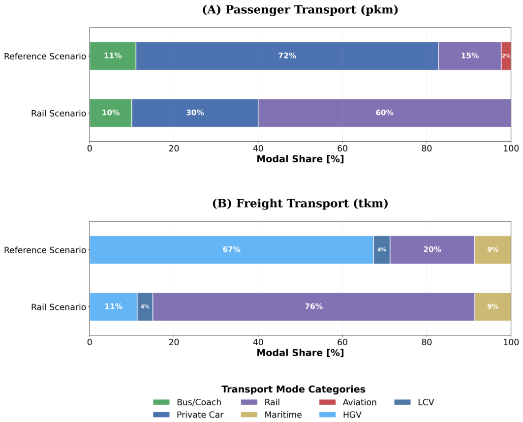
To evaluate the trade-offs between technology-oriented and structure-oriented transition strategies, we define two primary decarbonization pathways: the Reference Scenario, which follows institutional technology-substitution roadmaps, and the Rail Scenario, which prioritises structural modal shifts to mitigate biophysical constraints. To further isolate the impact of economic scale, each pathway is evaluated under two macroeconomic variants: a continuous growth case, aligned with official projections, and a Steady-State case, characterized by a transition toward macroeconomic stabilization. This dual-track approach allows for a rigorous assessment of how technological choices and macroeconomic paradigms interact to shape energy requirements, CO₂ emissions, monetary costs, and material demand through 2050. The fundamental differences in modal partition between the institutional paradigm and the rail transition are summarized in Figure 1. These configurations serve as the end-state targets for our simulations through 2050.

2.1.1. Reference Scenario: Institutional Green Growth (CETO 2025)

To establish a baseline trajectory compliant with institutional ambitions, we define a reference scenario based on the POTEnCIA model [22] and the CETO 2025 scenario [19], which operationalizes the targets of the European Climate Law [23,24]. As a proxy for the “Green Growth” paradigm, this pathway assumes absolute decoupling through rapid technological substitution and efficiency gains, projecting a 38% reduction in final energy consumption by 2050 despite continued economic expansion. While the strategy relies on pervasive road electrification—with battery electric vehicles exceeding 90% of the light-duty fleet—and the scale-up of renewable fuels, projections indicate a significant decarbonization lag where emissions do not fall below 1990 levels until 2032. We construct this reference within the pymedeas2 framework by adopting CETO technological and activity outputs as exogenous drivers, ensuring alignment with current EU climate policy while internalizing biophysical feedbacks for direct comparison with alternative structural pathways.

The Reference Scenario integrates institutional fuel-switching mandates for aviation and maritime sectors from ReFuelEU Aviation [25] and FuelEU Maritime [26] as projected in the CETO 2025 report [27]. Inland transport follows an electrification roadmap implementing the 2035 internal combustion engine phase-out, resulting in battery electric vehicles (BEVs) exceeding 90% of the passenger fleet by 2050. Freight dynamics reflect a heterogeneous transition with near-total electrification of Light Commercial Vehicles (LCVs) and a 2050 Heavy Goods Vehicle (HGV) mix of 66% BEVs and 20% hydrogen fuel cells [28]. Finally, rail activity growth is aligned with TEN-T expansion projections—84% for passengers and 68% for freight—to establish a consistent baseline for comparison with alternative modal shift strategies [29].

2.1.2. Alternative Pathway: Rail Scenario

The Rail Scenario operationalizes a structural shift from individual road mobility to electrified collective rail, building on the framework established by García-Olivares et al. [11]. Unlike technology-led substitution, this pathway targets the “decarbonization lag” inherent in the slow turnover of the European vehicle stock, which currently averages 12.5 and 14 years for passenger cars and heavy-duty vehicles, respectively [30]. The scenario simulates a fundamental reallocation of activity, projecting a 50–60% contraction of the private car fleet by 2050. Inland logistics follow an “All-Rail” logic, where road transport is capped at 15% of total ton-kilometers, reserved for last-mile distribution, while inter-urban freight is absorbed by electrified rail networks.

By 2050, rail transport reaches 100% electrification via overhead catenary systems, minimizing the need for large-scale battery storage. The remaining road fleet transitions entirely to electric propulsion for light-duty vehicles and buses. The freight transport segment (the 15% of activity remaining on road) operates on a mix of 90% battery or catenary-electric and 10% hydrogen fuel cells, with the latter strictly capped to preserve Platinum-group metal reserves.

2.1.3. Macroeconomic Variants: Growth vs. Steady-State Economy

To isolate the impact of structural modal shifts from the influence of total economic volume, each pathway described above is evaluated under two distinct macroeconomic trajectories. This dual-track approach generates four distinct scenarios (REF-G, REF-SSE, RAIL-G, and RAIL-SSE), allowing the pymedeas2 framework to capture the dynamic feedbacks between economic output, energy demand, and material constraints in a system-dynamics approach.

The first variant, the Growth trajectory (REF-G and RAIL-G), adopts the official macroeconomic projections aligned with the CETO 2025 and EU reference scenarios [31]. In this case, GDP per capita is assumed to follow a sustained growth trajectory through 2050. This variant serves as a “stress test” for technological and structural solutions: it evaluates whether deep electrification or radical modal shifts can remain biophysically feasible if the total volume of economic activity—and its associated mobility demand—continues to expand, as posited by proponents of green growth paradigms [7].

The second variant, the Steady-State Economy trajectory (REF-SSE and RAIL-SSE), implements a shift away from the paradigm of perpetual expansion [32]. In this trajectory, GDP per capita growth is parametrized to gradually decelerate, reaching zero by 2040 and remaining constant thereafter. This variant operationalizes the concept of sufficiency by reducing the activity pressure on the transport system, moving beyond mere technological efficiency [33]. By running the Rail Scenario under steady-state conditions (RAIL-SSE), we investigate the synergies between structural efficiency (trains) and demand-side sufficiency (macroeconomic stabilization), identifying the conditions necessary to stay within absolute planetary boundaries [34,35].

2.2. Modeling Framework

To analyze these scenarios, a new transport module has been integrated into the pymedeas2 model, employing a hybrid top–down and bottom–up approach to maintain metabolic consistency with the broader economy. Its structural logic follows a sequential causal chain: macroeconomic output drives aggregate demand for passenger (pkm) and freight (tkm) activity; this demand is subsequently disaggregated by mode and fuel share according to specific policy scenarios. Finally, these modal splits are coupled with technology-specific energy intensities and material intensity factors to quantify mineral requirements, total energy demand, and its associated CO₂ emissions, as detailed in Appendix B.1.

2.2.1. Transport Data Preprocessing and Demand Projection

Future transport activity trajectories are derived from econometric correlations with macroeconomic drivers, calibrated using historical data from the JRC-IDEES database [3]. We adopted a per-capita specification for passenger mobility and a GDP-centred model for freight to ensure mathematical consistency in the mature EU-27 economy. The projections follow a Constant Elasticity of Demand (CED) specification. To account for systemic inertia and temporal autocorrelation, the model incorporates a first-order autoregressive process (${\epsilon }_{t-1}$) derived from historical residuals. The resulting equations used for the system dynamics projections are:

$${\mathrm{PKM}}_t={\mathrm{PKM}}_0·exp\left[\gamma ln\left({\displaystyle \frac{{\mathrm{GDP}}_{\mathrm{pc},t}}{{\mathrm{GDP}}_{\mathrm{pc},0}}}\right)+\varphi {\epsilon }_{t-1}\right]$$

(1)

$${\mathrm{TKM}}_t={\mathrm{TKM}}_0·exp\left[\beta ln\left({\displaystyle \frac{{\mathrm{GDP}}_t}{{\mathrm{GDP}}_0}}\right)+\varphi {\epsilon }_{t-1}\right]$$

(2)

where $\gamma$ and $\beta$ represent the estimated income and freight elasticities, respectively. Parameters were estimated via Ordinary Least Squares (OLS) with Cochrane–Orcutt corrections, filtering pandemic-related anomalies (2020–2021) as exogenous shocks. The detailed regression framework, statistical diagnostics, and complete parameter tables are provided in Appendix C.

2.2.2. Material Demand and Economic Evaluation

The estimation of material requirements follows a two-step logic that translates transport demand into physical stocks. The required vehicle fleet size is first determined by applying vehicle intensity factors to the projected activity, accounting for historical occupancy rates and annual mileage. Subsequently, the modeling framework distinguishes between the active material stock in use and the annual demand required for maintenance and expansion. This mass-balance formulation, detailed in Appendix D.1, captures the total material throughput by accounting for both net fleet expansion and the replacement of degraded battery packs. Material intensity factors evolve dynamically through 2050 to reflect technological shifts, such as the transition toward Lithium Iron Phosphate (LFP) chemistries in passenger segments and the prioritization of high-nickel NCM 811 for heavy-duty logistics [36].

To evaluate the economic burden of the transition, we apply a physical capital replacement framework that disaggregates total annual investment into vehicle acquisition, charging infrastructure, and rail network expansion [11]. Vehicle investment covers both net expansion and the replacement of stock reaching the end of its operational life. The deployment of charging systems is parametrized following a high-utilization shared model that prioritizes fast-charging units to reduce the total material and spatial footprint of the network [37]. Finally, the structural shift toward rail necessitates significant investment in electrifying the remaining 46% of the current EU-27 network and constructing new tracks to absorb transferred road activity. The specific equations for material throughput and infrastructure costs across calculation methodology are documented in Appendix D.2. Crucially, our investment accounting captures only direct capital costs (fleet acquisition and primary track expansion). We explicitly exclude secondary expenses—such as maintenance, grid upgrades, and land acquisition—which require high-resolution spatial modeling outside our scope.

2.3. Data Integration and Calibration

The transport module is calibrated for the EU-27 using the JRC-IDEES 2023 database [3]. We aligned the model’s last historical year (2020) with empirical records of transport activity (pkm, tkm), vehicle stocks, and final energy demand (EJ). The calibration disaggregates the system by mode (m), fuel carrier (f), and technology (j).

2.3.1. Modal and Fuel Classification

Transport activity is disaggregated into passenger and freight sectors across the categories summarized in

Table 1. Classification and scope of transport modes included in the model.

Category	Mode	Scope and Inclusions
Passengers	Private Road	Individual cars and light-duty passenger vehicles
	Collective Road	Urban and interurban bus services
	Rail	High-speed, regional, and metropolitan networks
	Domestic Air	Internal flights within the modeled region
	Maritime	Regional ferries and passenger shipping
Freight	Road Heavy	Heavy goods vehicles (>3.5 t)
	Road Light	Light commercial vehicles (≤3.5 t)
	Rail	Electric and non-electric cargo trains
	Maritime	Short-sea shipping and inland waterways
	Air	Domestic cargo and logistical flights

. Energy demand is partitioned into four primary carriers: liquids (gasoline, diesel, LPG, and biofuels), gases (natural gas and bio-methane), electricity, and plug-in hybrids (PHEV). For PHEVs, the liquid and electric components are isolated to facilitate accurate energy substitution accounting. Within the freight sector, we maintain a structural distinction between Light Commercial Vehicles (LCVs ≤ 3.5 t) and Heavy Goods Vehicles (HGVs > 3.5 t) to account for their divergent energy intensities and load-optimized efficiencies [30].

2.3.2. Model Calibration and Performance Parameters

The module is calibrated for the EU-27 using the JRC-IDEES 2023 database [3]. We aligned the model’s base year (2020) with empirical records of transport activity (A), vehicle stocks (V), and energy demand (E) for each mode (m) and fuel (f). From this dataset, we derive the fuel-specific energy intensity ($e_{m,f}$) as the ratio of consumption to transport work:

$$e_{m,f}={\displaystyle \frac{E_{m,f}}{A_{m,f}}}$$

(3)

To link transport demand with material requirements, we calculate the annual vehicle productivity ($P_{m,f}$), representing the transport work performed per physical vehicle unit:

$$P_{m,f}={\displaystyle \frac{A_{m,f}}{V_{m,f}}}$$

(4)

The derivation of $P_{m,f}$ enables differentiated stock estimations based on specific battery capacities—such as 80 kWh for LCVs versus 600 kWh for HGVs—providing a more granular assessment of mineral requirements than fleet-wide averages [11].

3. Results

The simulation of the various decarbonization pathways reveals that technological shifts alone are insufficient to meet the EU’s 90% transport emission reduction target. Our analysis indicates that deep decarbonization requires a combined strategy of significant modal shift, high electrification, and substantial reduction in total activity volumes.

3.1. Passenger and Freight Metabolic Transition

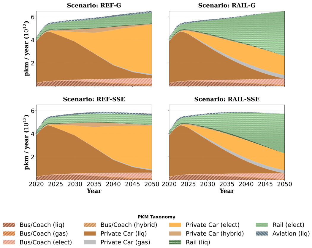
The transition matrices (Figure 2 and Figure 3) illustrate the divergent structural logic between institutional roadmaps and sufficiency-oriented strategies. In the passenger sector (Figure 2), Reference scenarios maintain a mobility system structurally reliant on individual vehicles, even with a near-total electrification of the light-duty fleet by 2050. In contrast, the Rail scenario implements a fundamental reallocation of activity, resulting in a 50–60% contraction of the private car fleet relative to baseline trends. By prioritizing high-speed electrified networks, rail becomes the primary carrier for medium-to-long distance travel by 2040.

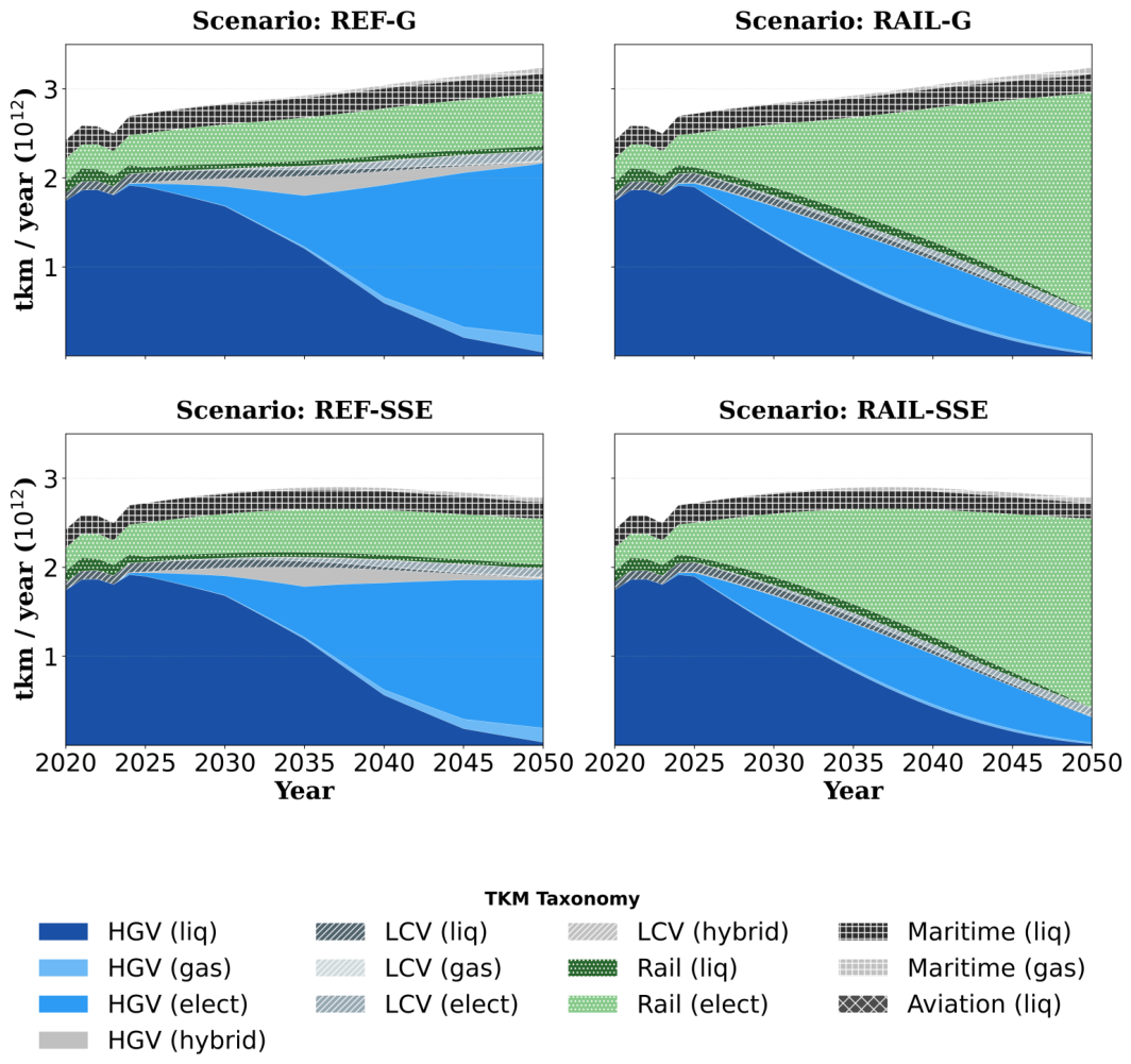
Regarding freight logistics (Figure 3), the Reference pathways sustain high activity levels for heavy goods vehicles (HGVs), which continue to dominate long-haul transport. The Rail scenario applies an “All-Rail” logic to inland logistics, effectively phasing out HGVs from the strategic bulk of inter-urban cargo. Under this framework, road transport is strictly reserved for capillary and last-mile distribution, limited to approximately 15% of total tkm.

The vertical differentiation across both matrices highlights the impact of macroeconomic scale. While structural shifts improve systemic efficiency, the Steady-State (SSE) variants effectively mitigate the demand-side pressure, preventing the activity growth projected under continuous economic expansion.

3.2. Transport Final Energy Demand

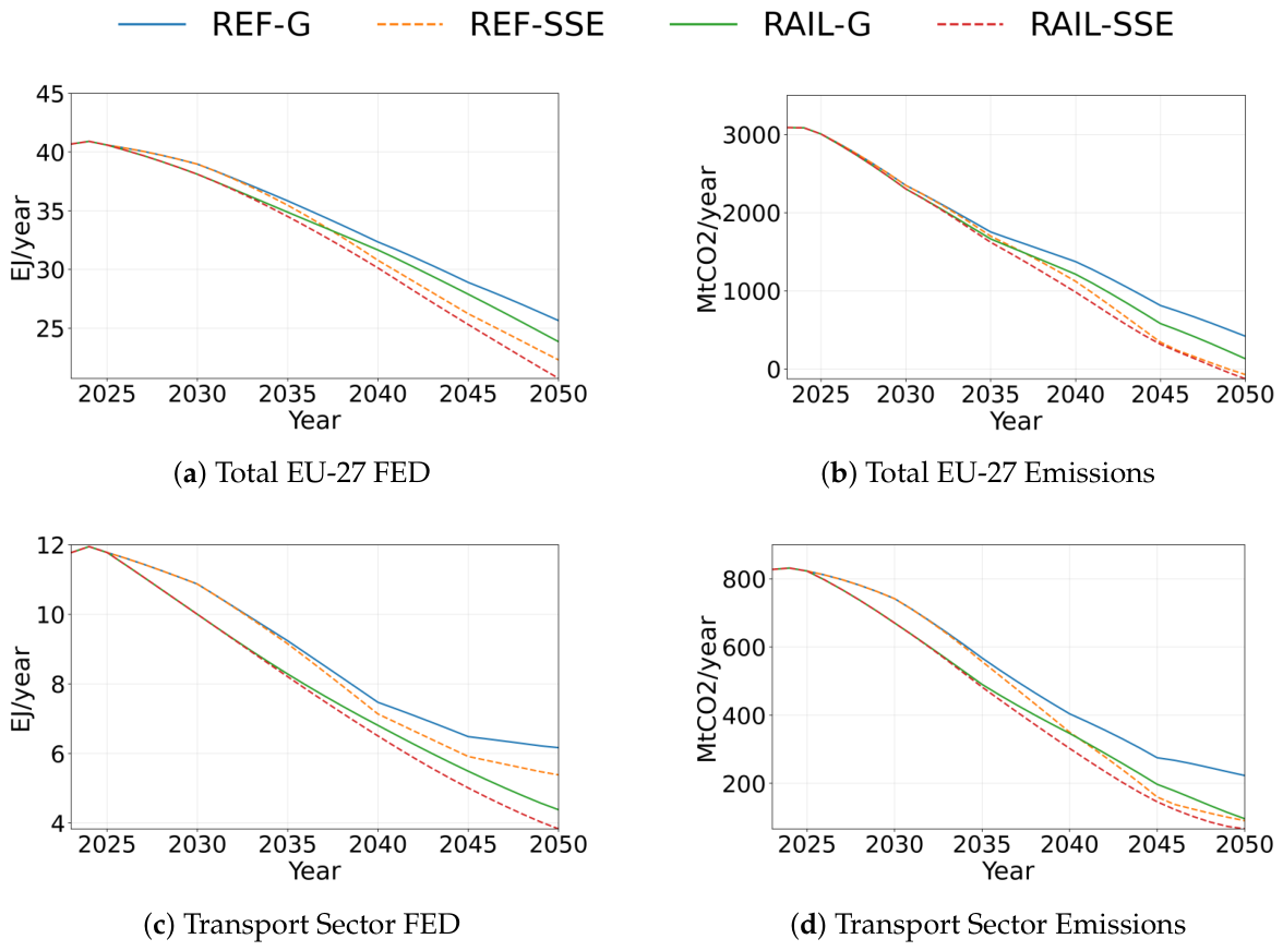
The simulation of Final Energy Demand (FED) reveals a clear divergence between the transport sector’s metabolism (Figure 4c) and the total EU-27 energy footprint (Figure 4a). From a common 2024 peak of 11.8 EJ in transport and approximately 41 EJ for the total socio-economy, the Reference Scenario pathways demonstrate the inherent limitations of a transition centered exclusively on technological substitution. While the superior thermodynamic efficiency of electric power-trains helps reduce transport demand to 6.2 EJ in the growth variant or 5.4 EJ under demand stabilization, these sectoral gains are partially neutralized by sustained mobility growth, resulting in a total EU-27 FED that remains as high as 26 EJ in the REF-G case. This trend underscores that maintaining an individual road-based mobility paradigm, even when electrified, sustains a metabolic inertia that significantly limits the overall reduction potential of the total economy.

In contrast, the Rail Scenario pathways illustrate how structural modal shifts fundamentally reshape both sectoral and systemic energy trajectories. The RAIL-SSE variant achieves an accelerated contraction, reaching 3.8 EJ in the transport sector—a 68% reduction from the 2024 peak—which in turn drives the total EU-27 FED to a systemic low of approximately 21 EJ by 2050. This deep reduction suggests that prioritizing high-capacity electrified rail over road-based alternatives acts as a superior thermodynamic leverage point, where modal substitution provides higher energy savings.

3.3. Decarbonization Trajectories and Emissions

The emission figures reported in this assessment represent operational and upstream energy CO₂ emissions, capturing direct vehicle operation and the carbon intensity of energy supply chains, while explicitly excluding the embodied carbon from vehicle manufacturing and large-scale infrastructure construction.

While all primary pathways achieve significant decarbonization by 2050, the trajectories for transport (Figure 4d) and the total EU-27 socio-economy (Figure 4b) diverge based on their specific structural and growth paradigms. In the transport sector, both Rail Scenario variants (RAIL-G and RAIL-SSE) achieve early action mitigation by bypassing the multi-decadal decarbonization lag inherent in private fleet turnover. However, the reduction in RAIL-G is partially limited by continued economic expansion, while the reference scenarios—even with the demand-side benefits of REF-SSE—remain fundamentally hampered by the high energy intensity of individual road-based mobility.

Consequently, the deepest absolute mitigation is achieved in the RAIL-SSE variant, where aggressive sectoral shifts and systemic sufficiency operate concurrently. Over the 2025–2050 time-frame, the institutional baseline (REF-G) results in cumulative transport emissions of 13.1 Gt CO₂, while the RAIL-SSE scenario restricts them to 10.6 Gt CO₂, reaching the lowest residual transport footprint of approximately 90 MtCO₂/year. This sectoral result is matched by the total socio-economic trajectory, which reflects the broader impact of a steady-state economy where GDP per capita growth reaches zero by 2040. Ultimately, the RAIL-SSE profile demonstrates that absolute sustainability requires reducing the physical scale of the entire economy alongside technological and modal transitions.

3.4. Cumulative Material Requirements: The Lithium Wall

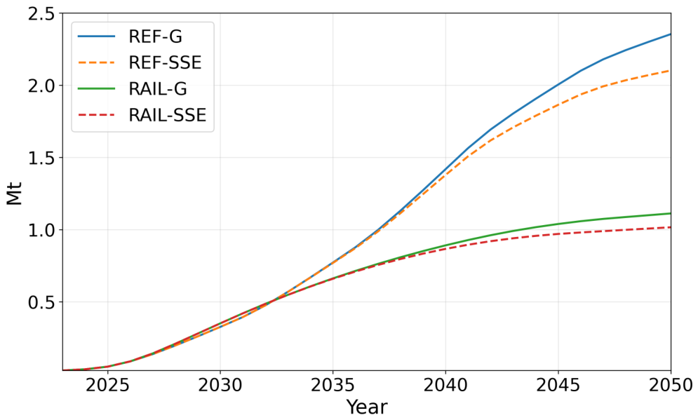
The biophysical feasibility of the evaluated pathways is primarily differentiated by the cumulative demand for Lithium (Figure 5). Under REF-G, the transition to a universal electric vehicle fleet, incorporating passenger cars, light commercial vehicles (LCVs), and heavy goods vehicles (HGVs), requires a cumulative extraction of approximately 2.35 million tons (Mt) of Lithium by 2050 [38]. These values represent the cumulative demand for metallic lithium. We acknowledge that the EU Battery Regulation (2023/1542) mandates ambitious lithium recovery targets of 50% by 2027 and 80% by 2031 [39]. However, due to the current lack of commercial-scale, high-efficiency closed-loop lithium recycling within the EU, and the inherent temporal lag between initial battery deployment and EoL availability, we explicitly frame our projections as a deliberately conservative upper bound for primary demand. Conversely, RAIL-SSE demonstrates a strategy for mineral parsimony, requiring only 1.02 Mt of Lithium over the same period, representing a 57% reduction relative to the baseline. By prioritizing catenary-powered rail and contracting the absolute volume of the private vehicle stock, this structural transition remains within safer biophysical boundaries while achieving superior decarbonization outcomes.

3.5. Economic Valuation: Capital Investment and Infrastructure Deployment

The economic assessment, summarized in

Table 2. Summary of cumulative investment and physical infrastructure deployment (2025–2050).

Indicator (Total 2025–2050)	REF-G	REF-SSE	RAIL-G	RAIL-SSE
Capital Investment (Trillion USD)
Private Vehicles	17.20	15.71	8.13	7.50
Buses	0.78	0.71	0.78	0.71
Freight Vehicles (LCV + HGV)	7.12	6.39	4.14	3.78
Rail Rolling Stock (Locomotives)	0.20	0.17	0.96	0.86
Charging Infrastructure ($I_{charge}$)	1.67	1.52	0.88	0.81
Rail Infrastructure (Tracks) ($I_{rail}$)	0.14	0.14	7.60	6.16
Total Investment ($I_{total}$)	27.10	24.64	22.50	19.83
Physical Deployment
New Rail Lines (km)	0	0	451,322	364,032
Rail Electrification (km)	108,784	108,784	108,784	108,784
AC Charging Posts (Millions)	91.82	83.68	48.39	44.43
DC Fast Chargers (Millions)	19.74	17.99	10.41	9.56

, reveals a profound structural divergence in capital allocation strategies between the evaluated pathways. Total cumulative investment is governed by a fundamental trade-off: the high-volume, continuous renewal of short-lived private vehicle fleets in the Reference Scenarios versus the infrastructure-intensive expansion of a durable rail network in the Rail Scenarios. In the REF-G scenario, capital expenditure is primarily driven by the private passenger fleet, which requires an investment of USD 17.20 trillion. Even under demand stabilization (REF-SSE), maintaining an individual mobility paradigm necessitates massive financial outflows totalling USD 15.71 trillion for private cars alone.

Conversely, the Rail Scenarios facilitate a substantial reduction in total vehicle-related capital by redirecting investment from individual machinery to high-capacity collective assets. The 50–60% contraction of the private car fleet and the phase-out of long-haul road freight effectively offset the increased investment required for electrified rail rolling stock. While investment in locomotives increases to between 0.96 and 0.86 trillion in these scenarios, the total capital required for road-based freight vehicles is nearly half that of the REF-G. Physical deployment further illustrates this shift; the RAIL-G requires planned public investment to construct 451,322 km of new high-speed and standard tracks, or 364,032 km in the more efficient RAIL-SSE variant.

Energy infrastructure costs further reflect the efficiency gains of the high-utilization shared model implemented in the Rail Scenarios. While the Reference Scenarios necessitate a fragmented network of nearly 112 million charging posts to support universal private electric vehicle ownership, the Rail Scenarios optimize expenditure, requiring fewer than 59 million units. Cumulatively, the RAIL-SSE variant emerges as the most economical pathway over the simulation period with a total investment of USD 19.83 trillion. This represents a systemic saving of USD 7.27 trillion relative to REF-G, demonstrating that the savings from avoided private vehicle acquisition and optimized charging networks compensate for the multi-trillion dollar costs of new track construction.

4. Discussion

This study applied the latest release of the pymedeas2 framework to assess the biophysical implications of the transport sector transition in the EU-27, aiming to evaluate which decarbonization pathways are most effective at minimizing structural dependencies on critical materials and overall energy demand. To achieve this, we contrasted four distinct scenarios: the institutional baseline (REF-G) focused on green growth and private fleet electrification; a rail-centric growth pathway (RAIL-G); a steady-state economy pathway maintaining road dominance (REF-SSE); and a sufficiency-driven pathway combining macroeconomic stabilization with rail expansion (RAIL-SSE). While all modeled pathways achieve significant decarbonization by 2050, the results demonstrate that institutional strategies like Reference Scenario remain unable to achieve the absolute decoupling of energy demand from transport activity. Although the superior thermodynamic efficiency of electric power-trains drives a downward trajectory in energy consumption across all scenarios—a trend consistent with official projections like the Clean Energy Technology Observatory [19]—these gains in Reference Scenario are partially neutralized by the sustained growth in transport volume. This confirms that a transition centred exclusively on fleet electrification maintains a high energy demand due to the metabolic inertia of persistent private vehicle usage, effectively limiting the scope of energy reduction to the efficiency of the delivery mechanism rather than the scale of the service provided.

In contrast, the RAIL-SSE scenario demonstrates that the integration of demand stabilization and structural modal shifts, specifically the transfer of long-distance activity to rail, acts as a superior thermodynamic leverage point. By bypassing the inherent energy intensity of individual road transport, these sufficiency-oriented pathways achieve an additional reduction in total energy consumption of approximately 39% relative to the reference. This divergence reveals that while technological substitution achieves a relative improvement, only the structural changes in Rail Scenario facilitate the absolute metabolic contraction required for biophysical sustainability. This outcome reinforces the theoretical critiques of the green growth paradigm offered by [7,8] while aligning with the demand-side mitigation strategies recently emphasized by the UNEP [40] and the European Scientific Advisory Board on Climate Change [41]. Both bodies increasingly emphasize that reaching climate neutrality necessitates structural reductions in energy service demand alongside rapid electrification.

The temporal dynamics of CO₂ mitigation reveal a persistent decarbonization lag in Reference Scenario pathways, highlighting the tension between market-led technological change and climate urgency. In these scenarios, the rate of emission reduction is fundamentally constrained by the physical inertia of the vehicle stock—an effect directly linked to the 12.5-year average age of the European passenger fleet [30]. This constraint implies that even if sales of internal combustion engines (ICEs) were phased out rapidly, the existing fleet would continue to consume the remaining carbon budget for over a decade. To contextualize the severity of this lag, deducting 2020–2024 historical emissions from the sector’s 1.5 °C-aligned budget [42] leaves a remaining allocation of strictly 6.4 to 8.3 Gt CO₂ from 2025 onward. Our modeling reveals that the REF-G trajectory drastically overshoots this biophysical limit by generating 13.1 Gt CO₂ in cumulative transport emissions, whereas the RAIL-SSE scenario restricts them to 10.6 Gt CO₂. While institutional frameworks often assume a near-linear decarbonization based on the market penetration of new electric vehicles [43], our results suggest that such projections frequently underestimate the “lock-in” effect of the current stock. This finding aligns with the warnings of Brand et al. [44], who argue that technological substitution alone is too slow to meet the 1.5 °C target, and reinforces observations by the European Environment Agency [45] that the ageing European fleet is becoming a structural barrier to rapid emission cuts; while other economic sectors are successfully decarbonizing, transport emissions remain high largely due to the slow turnover of the existing vehicle stock.

In contrast, the Rail Scenario serves as a temporal shortcut by decoupling decarbonization from the slow process of machine replacement. By enabling an immediate shift to existing electrified rail and reducing high-impact activities such as aviation, these pathways achieve deep systemic reductions long before the total electrification of the road fleet is physically possible. This structural intervention bypasses the multi-decadal turnover cycles that hamper Reference Scenario, delivering the early action mitigation [46] as essential for staying within biophysical limits. Although meeting the strictest 1.5 °C targets remains highly challenging even under the 10.6 Gt CO₂ trajectory, this structural pathway converges significantly closer to biophysical sustainability than technology-led green growth. Consequently, our analysis indicates that structural and demand-side measures likely play a fundamental role in achieving the rapid mitigation required by the Paris Agreement, suggesting that a technology-only approach may face significant temporal risks that these interventions could help mitigate.

Beyond the temporal and energetic risks, the physical feasibility of a technology-centric transition is challenged by extreme mineral intensity, creating a significant material bottleneck in the Reference Scenario pathways. Our results indicate that the cumulative lithium requirement for the EU-27 passenger fleet in the REF-G scenario reaches 2.35 million tons by 2050. While this constitutes approximately 6.4% of the 37 million tons of current global proven reserves [47], the fact that a single region representing less than 6% of the global population would claim this entire “fair share” solely for its domestic mobility calls into question the geopolitical and biophysical viability of a global green growth strategy [48]. Although circular economy strategies, including hydro-metallurgical recycling and secondary material recovery, are often proposed to mitigate these constraints, their current industrial scalability remains highly uncertain [49]. Furthermore, due to the inherent temporal lag between the initial deployment of battery stocks and their eventual EoL availability, secondary supply can only satisfy a fraction of the rapidly growing demand through 2050 [36]. Thus, while essential for long-term sustainability, circularity serves as a complementary improvement rather than a systemic solution to the resource-intensive requirements of the REF-G pathway, justifying a conservative assessment of primary demand.

This disproportionate appropriation becomes even more critical when accounting for competing cross-sectoral demands. Industry forecasts project that electric mobility will directly compete for lithium with the rapidly expanding stationary energy storage sector, which is indispensable for stabilizing renewable grids and relies heavily on lithium-intensive LFP chemistry [43,50]. Furthermore, this techno-centric dependence offshores significant environmental burdens; the energy-intensive extraction and refining processes generate substantial CO₂ emissions and ecological degradation outside the EU’s borders—typically in the Global South—a factor frequently externalised in institutional green growth accounting [38]. The aggressive electrification of private vehicles under REF-G effectively monopolizes the lithium required for both the EU’s own renewable grid and the basic energy needs of the rest of the world, suggesting that 1:1 vehicle replacement is structurally incompatible with a globally equitable transition. In contrast, the RAIL-SSE variant mitigates this risk by reducing cumulative lithium demand by 57%—to 1.02 Mt. This demonstrates that sufficiency and modal shifts act not only as transport mitigation strategies but as vital cross-sectoral resource-buffering mechanisms, essential to align the sector with the planet’s finite geological reality [38].

4.1. The Rail Transition as a Limit Case: Feasibility, Materiality, and Implementation Barriers

Despite the clear lithium demand advantages of the RAIL scenarios, the scale of infrastructure expansion required to absorb 60% of passenger and 76% of freight traffic presents profound real-world feasibility challenges. Our model indicates this shift would require an estimated 364,032 to 451,322 equivalent line-kilometers of new rail infrastructure. We explicitly frame these scenarios not as predictive forecasts, but as “limit cases” designed to analytically quantify the absolute biophysical boundaries of replacing road-dominated transport. While our macroeconomic framework captures the overarching capital and energy requirements, it does not account for micro-level operational factors such as traffic management, network capacity or specific operating modes. Furthermore, it does not account for protracted construction rates, specific land-use demand, or the complex spatial planning required to deploy new corridors. Absorbing such a massive reallocation of traffic would inevitably clash with protracted land-use planning processes and face significant hurdles regarding the social acceptance of extensive new construction projects [51].

Furthermore, this infrastructure-heavy pathway fundamentally shifts the material burden of the transition. While a rail-centred approach significantly reduces dependence on battery-grade lithium, it necessitates immense volumes of structural materials, such as copper for electrification and steel and cement for large-scale track construction. The associated embodied carbon represents an upfront emission penalty that may temporarily offset short-term climate gains [52,53]. However, this trade-off must be contextualized: the road-centric baseline is not exempt from these impacts, as it demands significant material inputs for highway maintenance and structural adaptation to accommodate heavier electric fleets. Consequently, rail expansion can trade the global supply-chain risks of battery metals for the localized, high-volume ecological impacts of heavy construction.

In light of these institutional, social, and physical barriers, our comparative analysis highlights the limitations of relying exclusively on either technology substitution or macro-structural modal shifts. While our aggregate EU-27 model abstracts from spatial specificities to identify absolute biophysical boundaries, realizing this transition requires unprecedented alignment across EU Member States [54]. In practice, transcending the binary between Green Growth and post-growth trajectories is essential. Policy must integrate sufficiency with systemic efficiency, optimizing transport architecture, dynamic flow management, and infrastructure utilization, alongside robust logistics reorganization and absolute transport demand reduction [55,56].

4.2. Macroeconomic Implications and Capital Reallocation

Finally, the divergence between these pathways translates into different macroeconomic requirements, where the Reference Scenarios represent a high capital expenditure transition that risks exacerbating the investment gap recently identified in assessments of European competitiveness [57]. By maintaining a growth-oriented activity model, this strategy necessitates a constant flow of capital into short-lived consumer goods—with the REF-G variant requiring USD 17.20 trillion for private vehicles alone, effectively crowding out investments in more durable public infrastructure.

In contrast, the Rail Scenarios suggest a shift in economic logic: by reducing the total volume of required machinery and prioritizing high-capacity rail, the transition moves from a consumption-heavy model toward a service-oriented one. While rail infrastructure investment rises to USD 6.16 trillion in the RAIL-SSE variant to support the construction of 364,032 km of new tracks, this expenditure is offset by the reduction in private vehicle acquisition costs to USD 7.50 trillion. Consequently, the RAIL-SSE pathway emerges as the most efficient strategy, requiring a total cumulative investment of USD 19.83 trillion, which represents a systemic saving of USD 7.27 trillion relative to the REF-G baseline. This alignment with post-growth frameworks [8,58] suggests that absolute sustainability is only achievable if the European economy is reoriented away from resource-intensive GDP growth and toward the provision of essential services with minimal biophysical and capital overhead.

5. Conclusions

This study demonstrates that, under the modeled assumptions of high-growth baselines, conventional technology-led pathways succeed in improving relative efficiency but face significant challenges in achieving the absolute energy reduction required for sustainability due to the metabolic inertia of transport demand within the EU-27. We frame our RAIL-SSE scenarios as normative limit-cases rather than predictive forecasts, designed to analytically quantify the biophysical boundaries of a post-growth transition. Consequently, our analysis indicates that transport decarbonization likely requires more than technological substitution; an absolute reduction in the physical scale of activity, quantified as the aggregate annual volume of $pkm$ and $tkm$, appears to be a fundamental factor in achieving biophysical sustainability.

First, the temporal dynamics of CO₂ mitigation reveal a persistent decarbonization lag, where the 12.5-year average age of the European passenger fleet acts as a structural barrier to rapid emission cuts. Assuming this current lifespan remains constant, the high average age of the European fleet creates a multi-decadal lag that market-driven electrification cannot overcome in time to meet climate targets. Only a large-scale modal shift toward electrified rail and demand-side management can bypass these vehicle turnover cycles, providing the immediate emission reductions necessary to remain within biophysical limits.

Second, universal private electrification presents significant challenges regarding resource equity under current demand growth assumptions and life-cycle material intensities. An EU-27 private electric fleet would require 2.35 million tons of lithium by 2050, claiming 6.4% of global reserves for only the transport sector of a region with only 6% of the world’s population. This concentration of resources is structurally incompatible with a globally equitable transition. Conversely, the RAIL-SSE scenario reduces cumulative lithium demand by 57%, aligning the sector with the reality of finite geological endowments.

Third, when assessed within the defined system boundaries that focus on direct capital requirements for fleet and basic network expansion, a structure-led transition proves to be economically superior to technology-led green growth. Despite the massive upfront capital required to expand and electrify the European rail network, the RAIL-SSE pathway emerges as the least capital-intensive strategy. By drastically reducing the continuous, high-volume acquisition of short-lived private vehicles and optimizing charging infrastructure, this sufficiency-driven scenario yields a systemic saving of over USD 7.27 trillion relative to the institutional baseline.

From a policy perspective, the divergence in metabolic and economic pathways indicates that absolute sustainability necessitates aligning EU policy with post-growth frameworks, prioritizing durable public infrastructure and service provision over resource-intensive GDP expansion. Future policy should integrate sufficiency as a core pillar alongside efficiency and renewables to mitigate the identified temporal and material risks and ensure a resilient transition within the sector’s absolute biophysical limits. To advance this paradigm, future research must expand this integrated framework to assess the socio-economic distributional impacts of sufficiency-based transitions, particularly concerning employment shifts and equity. Furthermore, deepening the analysis of circular economy strategies—such as secondary material recovery and alternative battery chemistries—is essential to further refine the mitigation of the material constraints identified in this study.

References

1. European Commission; Joint Research Centre (JRC); International Energy Agency (IEA). EDGAR (Emissions Database for Global Atmospheric Research) Community GHG Database, Version EDGAR_2025_GHG; European Commission, JRC (Datasets): Ispra, Italy, 2025. [Google Scholar]
2. Crippa, M.; Guizzardi, D.; Pagani, F.; Banja, M.; Muntean, M.; Schaaf, E.; Quadrelli, R.; Risquez Martin, A.; Taghavi-Moharamli, P.; Köykkä, J.; et al. GHG Emissions of All World Countries—2025 Report; Technical Report JRC143227; Publications Office of the European Union: Luxembourg, 2025. [Google Scholar] [CrossRef]
3. Rozsai, M.; Jaxa-Rozen, M.; Salvucci, R.; Sikora, P.; Gea Bermudez, J.; Neuwahl, F. JRC-IDEES-2023. European Commission, Joint Research Centre (JRC) [Dataset]. 2025. Available online: http://data.europa.eu/89h/1f0b480c-6d21-4d95-897d-20c7ca33df6f (accessed on 13 July 2026).
4. Transport and Environment. Europe’s Transport Sector Set to Make Up Almost Half of the Continent’s Emissions in 2030; Policy Analysis; Transport and Environment: Brussels, Belgium, 2024. [Google Scholar]
5. European Commission. The European Green Deal; COM(2019) 640 Final; European Commission: Brussels, Belgium, 2019. [Google Scholar]
6. European Commission. Communication from the Commission to the European Parliament, the Council, the European Economic and Social Committee and the Committee of the Regions. ’Fit for 55’: Delivering the EU’s 2030 Climate Target on the Way to Climate Neutrality; European Commission: Brussels, Belgium, 2021. [Google Scholar]
7. Hickel, J.; Kallis, G. Is Green Growth Possible? New Political Econ. 2020, 25, 469–486. [Google Scholar] [CrossRef]
8. Parrique, T.; Barth, J.; Briens, F.; Kerschner, C.; Kraus-Polk, A.; Magee, A.; Spangenberg, J.H. Decoupling Debunked: Evidence and Arguments Against Green Growth as a Sole Strategy for Sustainability; Technical report; European Environmental Bureau (EEB): Brussels, Belgium, 2019. [Google Scholar]
9. Wiedmann, T.; Lenzen, M.; Keyßer, L.T.A.; Steinberger, J.K. Scientists’ warning on affluence. Nat. Commun. 2020, 11, 3107. [Google Scholar] [CrossRef] [PubMed]
10. García-Olivares, A.; Solé, J.; Osychenko, O. Transportation in a 100% renewable energy system. Energy Convers. Manag. 2018, 158, 266–285. [Google Scholar] [CrossRef]
11. García-Olivares, A.; Solé, J.; Samsó, R.; Ballabrera-Poy, J. Sustainable European Transport System in a 100% Renewable Economy. Sustainability 2020, 12, 5091. [Google Scholar] [CrossRef]
12. Valero, A.; Valero, A.; Calvo, G.; Ortego, A. Material bottlenecks in the future development of green technologies. Renew. Sustain. Energy Rev. 2018, 93, 178–200. [Google Scholar] [CrossRef]
13. Alcover, E.; Mas, B.; Martínez-Moll, V.; Rosselló, J.L.; Roca, M.; Canals, V. Energetic and economic analysis of the Electric Vehicles charge impacts on public parking lots. Renew. Energy Power Qual. J. (REandPQJ) 2020, 18, 741–746. [Google Scholar] [CrossRef]
14. Creutzig, F.; Niamir, L.; Bai, X.; Callaghan, M.; Cullen, J.; Díaz-José, J.; Figueroa, M.; Grübler, A.; Lamb, W.; Leip, A.; et al. Demand, Services and Social Aspects of Mitigation. In Climate Change 2022: Mitigation of Climate Change. Contribution of Working Group III to the Sixth Assessment Report of the Intergovernmental Panel on Climate Change; Cambridge University Press: Cambridge, UK; New York, NY, USA, 2022. [Google Scholar] [CrossRef]
15. Solé, J.; Samsó, R.; García-Ladona, E.; García-Olivares, A.; Ballabrera-Poy, J.; Madurell, T.; Turiel, A.; Osychenko, O.; Álvarez, D.; Bardi, U.; et al. modeling the renewable transition: Scenarios and pathways for a decarbonized future using pymedeas, a new open-source energy systems model. Renew. Sustain. Energy Rev. 2020, 132, 110105. [Google Scholar] [CrossRef]
16. Michaux, S.P. Assessment of the Extra Capacity Required of Alternative Energy Electrical Power Systems to Completely Replace Fossil Fuels; Open File Report 42/2021; Geological Survey of Finland (GTK): Espoo, Finland, 2021. [Google Scholar] [CrossRef]
17. Muratori, M. Impact of uncoordinated plug-in electric vehicle charging on residential power demand. Nat. Energy 2018, 3, 193–201. [Google Scholar] [CrossRef]
18. Alsharif, A.; Tan, C.; Ayop, R.; Al Smin, A.; Ali Ahmed, A.; Kuwil, F.; Khaleel, M. Impact of Electric Vehicle on Residential Power Distribution Considering Energy Management Strategy and Stochastic Monte Carlo Algorithm. Energies 2023, 16, 1358. [Google Scholar] [CrossRef]
19. Neuwahl, F.; Wegener, M.; Salvucci, R.; Jaxa-Rozen, M.; Gea Bermudez, J.; Sikora, P.; Rózsai, M. Clean Energy Technology Observatory: POTEnCIA CETO 2025 Scenario; Publications Office of the European Union: Luxembourg, 2025. [Google Scholar] [CrossRef]
20. Alcover Comas, E.; Guardia Calsina, P.; Samsó, R.; Solé, J. Exploring decarbonisation strategies in the Southern-European region of Catalonia through a multi-scenario assessment. Energy Strategy Rev. 2026, 64, 102184. [Google Scholar] [CrossRef]
21. Stadler, K.; Wood, R.; Bulavskaya, T.; Södersten, C.J.; Simas, M.; Schmidt, S.; Usubiaga, A.; Acosta-Fernández, J.; Kuenen, J.; Bruckner, M.; et al. EXIOBASE 3: Developing a Time Series of Detailed Environmentally Extended Multi-Regional Input-Output Tables. J. Ind. Ecol. 2018, 22, 502–515. [Google Scholar] [CrossRef]
22. Mantzos, L.; Wiesenthal, T. POTEnCIA Model Description, Version 0.9; Publications Office of the European Union: Luxembourg, 2016. [CrossRef]
23. European Union. Regulation (EU) 2021/1119 of the European Parliament and of the Council of 30 June 2021 establishing the framework for achieving climate neutrality and amending Regulations (EC) No 401/2009 and (EU) 2018/1999 (European Climate Law). Off. J. Eur. Union 2021, L 243, 1–17. [Google Scholar]
24. European Commission. Securing Our Future Europe’s 2040 Climate Target and Path to Climate Neutrality by 2050 Building a Sustainable, Just and Prosperous Society; Technical Report COM(2024) 63 final; European Commission: Brussels, Belgium, 2024. [Google Scholar]
25. European Parliament and Council. Regulation (EU) 2023/2405 on ensuring a level playing field for sustainable air transport (ReFuelEU Aviation). Off. J. Eur. Union 2023, L 243, 1–30. [Google Scholar]
26. European Parliament and Council. Regulation (EU) 2023/1805 on the use of renewable and low-carbon fuels in maritime transport (FuelEU Maritime). Off. J. Eur. Union 2023, L 243, 48–100. [Google Scholar]
27. Buffi, M.; Motola, V.; Rejtharova, J.; Hurtig, O.; Scarlat, N.; Mountraki, A.; Georgakaki, A.; Salvucci, R.; Schade, B.; Rózsai, M.; et al. Clean Energy Technology Observatory: Renewable Fuels of Non-Biological Origin in the European Union—2025 Status Report on Technology Development, Trends, Value Chains and Markets; Publications Office of the European Union: Luxembourg, 2025. [Google Scholar] [CrossRef]
28. European Parliament and Council. Regulation (EU) 2024/1610 amending Regulation (EU) 2019/1242 as regards strengthening the CO2 emission performance standards for new heavy-duty vehicles and integrating reporting obligations, amending Regulation (EU) 2018/858 and repealing Regulation (EU) 2018/956 (Text with EEA relevance). Off. J. Eur. Union 2024, L 243, 1–67. [Google Scholar]
29. European Commission. Revised TEN-T Regulation and Infrastructure for Sustainable Mobility: Impact Assessment and Projections; Technical report; Directorate-General for Mobility and Transport (DG MOVE): Brussels, Belgium, 2024. [Google Scholar]
30. ACEA. Report: Vehicles on EUROPEAN Roads 2025; Technical report; European Automobile Manufacturers’ Association: Brussels, Belgium, 2025. [Google Scholar]
31. European Commission. EU Reference Scenario 2024: Energy, Transport and GHG Emissions—Trends to 2050; Technical report; Directorate-General for Energy, DG Climate Action and DG Mobility and Transport: Brussels, Belgium, 2024. [Google Scholar]
32. Daly, H.E. Steady-State Economics: Second Edition with New Essays; Island Press: Washington, DC, USA, 1991. [Google Scholar]
33. Zell-Ziegler, C.; Thema, J.; Best, B.; Wiese, F.; Lage, J.; Schmidt, A.; Toulouse, E.; Stagl, S. Enough? The role of sufficiency in European energy and climate plans. Energy Policy 2021, 157, 112483. [Google Scholar] [CrossRef]
34. Steffen, W.; Richardson, K.; Rockström, J.; Cornell, S.E.; Fetzer, I.; Bennett, E.M.; Biggs, R.; Carpenter, S.R.; de Vries, W.; de Wit, C.A.; et al. Planetary boundaries: Guiding human development on a changing planet. Science 2015, 347, 1259855. [Google Scholar] [CrossRef] [PubMed]
35. O’Neill, D.W.; Fanning, A.L.; Lamb, W.F.; Steinberger, J.K. A good life for all within planetary boundaries. Nat. Sustain. 2018, 1, 88–95. [Google Scholar] [CrossRef]
36. Xu, C.; Dai, Q.; Gaines, L.; Hu, M.; Tukker, A.; Steubing, B. Future material demand for automotive lithium-based batteries. Commun. Mater. 2020, 1, 99. [Google Scholar] [CrossRef]
37. Xylia, M.; Olsson, E.; Macura, B.; Nykvist, B. Estimating charging infrastructure demand for electric vehicles: A systematic review. Energy Strategy Rev. 2025, 59, 101753. [Google Scholar] [CrossRef]
38. Valero, A.; Valero, A.; Calvo, G. The Material Limits of Energy Transition: Thanatia; Springer: Cham, Switzerland, 2023. [Google Scholar] [CrossRef]
39. European Parliament and Council of the European Union. Regulation (EU) 2023/1542 of the European Parliament and of the Council of 12 July 2023 concerning batteries and waste batteries, amending Directive 2008/98/EC and Regulation (EU) 2019/1020 and repealing Directive 2006/66/EC. Off. J. Eur. Union 2023, L 191, 1–117. [Google Scholar]
40. United Nations Environment Programme. Emissions Gap Report 2024: No More Hot Air … Please! Technical report; UNEP: Nairobi, Kenya, 2024. [Google Scholar]
41. European Scientific Advisory Board on Climate Change. Towards EU Climate Neutrality: Progress, Policy Gaps and Opportunities; Technical report; European Environment Agency: Copenhagen, Denmark, 2024.
42. Plötz, P.; Wachsmuth, J.; Gnann, T. Net-Zero-Carbon Transport in Europe Until 2050—Targets, Technologies and Policies for a Long-Term EU Strategy; Technical report; Fraunhofer Institute for Systems and Innovation Research (ISI): Karlsruhe, Germany, 2021. [Google Scholar]
43. International Energy Agency. Global EV Outlook 2026: Growing Sales Amid an Energy Crisis; Technical report; IEA: Paris, France, 2026. [Google Scholar]
44. Brand, C.; Götschi, T.; Dons, E.; Gerike, R.; Anaya-Boig, E.; Avila-Palencia, I.; de Nazelle, A.; Gascon, M.; Gaupp-Berghausen, M.; Iacorossi, F.; et al. The climate change mitigation impacts of active travel: Evidence from a longitudinal panel study in seven European cities. Glob. Environ. Change 2021, 67, 102224. [Google Scholar] [CrossRef]
45. European Environment Agency. Trends and Projections in Europe 2024; EEA Report 08/2024; EEA: Copenhagen, Denmark, 2024. [Google Scholar]
46. Grubler, A.; Wilson, C.; Bento, N.; Boza-Kiss, B.; Krey, V.; McCollum, D.L.; Rao, N.D.; Riahi, K.; Rogelj, J.; De Stercke, S.; et al. A low energy demand scenario for meeting the 1.5 °C target and sustainable development goals without negative emission technologies. Nat. Energy 2018, 3, 515–527. [Google Scholar] [CrossRef]
47. U.S. Geological Survey. Mineral Commodity Summaries 2026; Technical report; U.S. Geological Survey: Reston, VA, USA, 2026. [CrossRef]
48. Goonan, T.G. Lithium Use in Batteries; Technical Report 1371; U.S. Geological Survey: Reston, VA, USA, 2012. [CrossRef]
49. Harper, G.; Sommerville, R.; Kendrick, E.; Driscoll, L.; Slater, P.; Stolkin, R.; Walton, A.; Christensen, P.; Heidrich, O.; Lambert, S.; et al. Recycling lithium-ion batteries from electric vehicles. Nature 2019, 575, 75–86. [Google Scholar] [CrossRef] [PubMed]
50. Gregoir, L.; van Acker, K. Metals for Clean Energy: Pathways to Solving Europe’s Raw Materials Challenge; Technical report; KU Leuven: Leuven, Belgium, 2022. [Google Scholar]
51. Flyvbjerg, B. Policy and Planning for Large-Infrastructure Projects: Problems, Causes, Cures. Environ. Plan. B Plan. Des. 2007, 34, 578–597. [Google Scholar] [CrossRef]
52. Hausberger, L.; Cordes, T.; Gschösser, F. Life Cycle Assessment of High-Performance Railway Infrastructure, Analysis of Superstructures in Tunnels and on Open Tracks. Sustainability 2023, 15, 7064. [Google Scholar] [CrossRef]
53. Knabl, D.; Landgraf, M. In-Depth Lifecycle Assessment of Ballasted Railway Track and Slab Track Considering Varying Subsoil Conditions. Sustainability 2023, 15, 12974. [Google Scholar] [CrossRef]
54. Boira, J.V.; Berzi, M. Liberalization, Trans-European Corridors and EU Funds: A New Scenario in the Relationship between Rail Networks and Mediterranean Cities. Land 2023, 12, 1986. [Google Scholar] [CrossRef]
55. Creutzig, F.; Roy, J.; Lamb, W.F.; Azevedo, I.M.L.; de Bruin, W.B.; Dalkmann, H.; Edelenbosch, O.Y.; Geels, F.W.; Grubler, A.; Hepburn, C.; et al. Towards demand-side solutions for mitigating climate change. Nat. Clim. Change 2018, 8, 260–263. [Google Scholar] [CrossRef]
56. Jarre, M.; Noussan, M.; Campisi, E. Avoid–Shift–Improve: Are Demand Reduction Strategies Under-Represented in Current Energy Policies? Energies 2024, 17, 4955. [Google Scholar] [CrossRef]
57. Draghi, M. The Future of European Competitiveness; Technical report; European Commission: Brussels, Belgium, 2024. [Google Scholar] [CrossRef]
58. Jackson, T. Post Growth: Life After Capitalism; Polity Press: Cambridge, UK, 2021. [Google Scholar]
59. Morris, M.D. Factorial sampling plans for preliminary computational experiments. Technometrics 1991, 33, 161–174. [Google Scholar] [CrossRef]
60. Saltelli, A.; Ratto, M.; Andres, T.; Campolongo, F.; Cariboni, J.; Gatelli, D.; Saisana, M.; Tarantola, S. Global Sensitivity Analysis: The Primer; John Wiley and Sons: Hoboken, NJ, USA, 2007. [Google Scholar] [CrossRef]
61. Herman, J.; Usher, W. SALib: An open-source Python library for sensitivity analysis. J. Open Source Softw. 2017, 2, 97. [Google Scholar] [CrossRef]
62. Samsó, R.; De Blas, I.; Perissi, I.; Martelloni, G.; Solé, J. Scenario analysis and sensitivity exploration of the MEDEAS Europe energy-economy-environment model. Energy Strategy Rev. 2020, 32, 100582. [Google Scholar] [CrossRef]
63. Hickel, J.; Brockway, P.; Kallis, G.; Keyßer, L.; Lenzen, M.; Slameršak, A.; Steinberger, J.; Ürge-Vorsatz, D. Urgent need for post-growth climate mitigation scenarios. Nat. Energy 2021, 6, 766–768. [Google Scholar] [CrossRef]
64. International Energy Agency (IEA). World Energy Outlook 2025 Extended Dataset; Licence: Terms of Use for Non-CC Material; International Energy Agency (IEA): Paris, France, 2025. [Google Scholar]
65. Rasul, K.; Schmidt, S.; Hertwich, E.G.; Wood, R. EXIOBASE energy accounts: Improving precision in an open-sourced procedure applicable to any MRIO database. J. Ind. Ecol. 2024, 28, 1771–1785. [Google Scholar] [CrossRef]
66. Hyndman, R.J.; Athanasopoulos, G. Forecasting: Principles and Practice, 2nd ed.; OTexts: Melbourne, Australia, 2018. [Google Scholar]
67. Neidhardt, M.; Mas-Peiro, J.; Schulz-Moenninghoff, M.; Pou, J.O.; Gonzalez-Olmos, R.; Kwade, A.; Schmuelling, B. Forecasting the Global Battery Material Flow: Analyzing the Break-Even Points at Which Secondary Battery Raw Materials Can Substitute Primary Materials. Appl. Sci. 2022, 12, 4790. [Google Scholar] [CrossRef]
68. Danielis, R.; Niazi, A.M.K.; Scorrano, M.; Masutti, M.; Awan, A.M. The Economic Feasibility of Battery Electric Trucks: A Review of the Total Cost of Ownership Estimates. Energies 2025, 18, 429. [Google Scholar] [CrossRef]
69. Ghotge, R.; van Rooij, D.; van Breukelen, S. Total Cost of Ownership of Electric Buses in Europe. World Electr. Veh. J. 2025, 16, 464. [Google Scholar] [CrossRef]
70. Research and Markets. Electric Locomotives Market Size, Share and Forecast; Technical report; Research and Markets: Dublin, Ireland, 2026. [Google Scholar]
71. Nicholas, M.; Hall, D. Lessons Learned on Charging Infrastructure Costs and Deployment; Technical report; International Council on Clean Transportation (ICCT): Washington, DC, USA, 2022. [Google Scholar]
72. Wood, E.; Borlaug, B.; Moniot, M.; Lee, D.-Y.; Ge, Y.; Yang, F.; Liu, Z. The 2030 National Charging Network: Estimating U.S. Light-Duty Demand for Electric Vehicle Charging Infrastructure; Technical Report NREL/TP-5400-85654; National Renewable Energy Laboratory (NREL): Golden, CO, USA, 2023. [CrossRef]
73. Hao, H.; Geng, Y.; Tate, J.E.; Liu, Z.; Sun, X.; Mu, Z.; Sun, L.; Zhao, F. Impact of transport electrification on critical metal sustainability with a focus on the heavy-duty segment. Nat. Commun. 2019, 10, 5398. [Google Scholar] [CrossRef] [PubMed]
74. Wagner, D.; Walther, G. Techno-economic analysis of mixed battery and fuel cell electric bus fleets: A case study. Appl. Energy 2024, 376, 124285. [Google Scholar] [CrossRef]
75. Mordor Intelligence. Electric Bus Battery Market Size and Share Analysis—Growth Trends and Forecasts (2024–2029); Market research report; Mordor Intelligence: Telangana, India, 2024. [Google Scholar]
Figure 1. Structural archetypes for the 2050 transport system. Panel A illustrates the passenger modal split (pkm), highlighting the transition from private vehicle dominance in the Reference Scenario to a rail-centric collective system. Panel B displays the freight modal split (tkm), where the Rail Scenario applies an “all-rail” logic to long-haul logistics, reserving road transport (LCV) primarily for capillary distribution. Note that while absolute activity volumes vary between Growth (-G) and Steady-State (-SSE) variants, these modal shares define the structural logic of each pathway.
Sustainability 18 07402 g001
Figure 2. Evolution of Passenger Transport Demand and Modal Share (2020–2050). The projections illustrate distinct transition pathways, contrasting institutional technology substitution with structural modal shifts under two macroeconomic paradigms.
Sustainability 18 07402 g002
Figure 3. Evolution of Freight Transport Demand and Modal Share (2020–2050). The projections illustrate a structural shift, replacing road-based long-haul freight with electrified rail networks under the two macroeconomic scenarios.
Sustainability 18 07402 g003
Figure 4. Evolution of Final Energy Demand (FED) and CO2 emissions (2020–2050). (a) Total EU-27 FED, capturing the systemic effects of transport modal shifts and macroeconomic stabilization; (b) Total CO2 emissions, showing the synergy between modal shifts and macroeconomic stabilization; (c) Transport sector’s FED evolution, contrasting the gradual reduction in Reference pathways with the Rail variats; (d) Transport-related emissions, highlighting the decarbonization lag of technology-centric scenarios.
Sustainability 18 07402 g004
Figure 5. Cumulative Lithium requirements for EV batteries through 2050. The results contrast the material intensity of private fleet electrification (REF-G and REF-SSE) with the mineral parsimony of structural modal shifts (RAIL-G and RAIL-SSE).
Sustainability 18 07402 g005