Fully Transient Analytical Solutions for Organic Contaminant Transport Through GMB/CCL and GMB/GCL Composite Liners Considering Advection, Degradation and Thermodiffusion for Sustainable Mitigation

Abstract

This paper presents fully transient analytical solutions for organic contaminant transport through composite liner systems consisting of a geomembrane (GMB) underlain by either a compacted clay liner (CCL) or a geosynthetic clay liner (GCL). The proposed solutions simultaneously account for three key mechanisms, namely advection due to GMB defects and wrinkles, first-order degradation, and thermodiffusion induced by temperature gradients. The solutions provide steady-state temperature distribution, transient contaminant concentration profiles, mass flux, and cumulative mass outflow at the base of the liner. The analytical solutions are rigorously verified against experimental thermodiffusion data from the literature, an existing analytical solution, and a numerical model using COMSOL Multiphysics 5.4. A parametric study is conducted to investigate the effects of thermodiffusion, Soret coefficient, and thermal conductivity on benzene transport. Results show that thermodiffusion substantially increases benzene outflow; neglecting it may lead to unconservative liner design. The benzene transport rate increases almost linearly with the Soret coefficient. The thermal conductivity of the GMB and GCL significantly affects benzene transport in the GMB/GCL system, while the thermal conductivities of the GMB and CCL have negligible effects on the GMB/CCL system. The proposed analytical solutions enable rapid parametric analysis, preliminary liner design, environmental risk assessment, and early warning. By enabling rapid comparison of GMB/CCL versus GMB/GCL systems (material selection), optimization of clay layer thickness for required breakthrough time (thickness optimization), and quantification of thermal effects on contaminant flux (temperature control), the solutions serve as an efficient tool for sustainable liner design.

1. Introduction

Bottom liner systems consisting of a geomembrane (GMB) underlain by either a compacted clay liner (CCL) or a geosynthetic clay liner (GCL) are widely used in modern municipal solid waste landfills to isolate waste and leachate from the surrounding environment [1,2,3]. Although such GMB-based composite liners are effective, organic contaminants can still diffuse through intact GMBs [4,5]. Moreover, defects and wrinkles are commonly present in GMBs even under strict construction quality assurance programs [6,7]. Advection through these defects can significantly enhance contaminant migration, especially when a high leachate head and many defects exist [8,9,10,11]. In addition, degradation has been recognized as a key attenuation process for organic contaminants in clay liners [12,13,14].

Numerous analytical and numerical models have been developed to predict organic contaminant transport in liner systems considering molecular diffusion, advection, and degradation [9,10,11,15,16,17]. However, most of these studies have been conducted under isothermal conditions, neglecting the fact that landfills often experience elevated temperatures due to waste degradation or hydration of incinerated ash. Temperatures in landfill liners can reach 50–70 °C [18,19,20] and even up to 80 °C in mining applications [21]. Such thermal gradients induce thermodiffusion (Soret effect), which can drive additional contaminant mass flux comparable to molecular diffusion [22,23]. Experimental evidence has confirmed that thermodiffusion enhances solute transport in compacted clays [23]. Therefore, a reliable assessment of liner performance must account for the combined effects of advection through GMB defects, degradation, and thermodiffusion.

In recent years, several studies have incorporated thermodiffusion into analytical models for liner systems. Xie et al. [24] presented an analytical model for chemical diffusion under thermal effects in semi-infinite porous media. Yan et al. [25] derived analytical solutions for thermally induced diffusion under steady-state heat transfer. Peng et al. [26] developed an analytical model for organic contaminant transport through a GMB/CCL composite liner, including thermodiffusion but without considering GMB defects or degradation. More recently, Qiu et al. [27] proposed analytical solutions for a GMB/GCL/CCL triple-layer liner under non-isothermal conditions, accounting for temperature-dependent diffusion and partition coefficients; nevertheless, advection due to GMB defects was neglected. Qiu et al. [28] provided analytical solutions for a GMB/CCL composite liner that incorporated GMB defects, effective porosity, and thermodiffusion, but degradation was not included. Meanwhile, numerical solutions capable of handling transient heat transfer and temperature-dependent properties (e.g., [29,30]) have been developed, but they are not as convenient for rapid parametric studies or for use as benchmarking tools.

However, no analytical solution has been reported that simultaneously considers (i) advection due to GMB defects/wrinkles, (ii) first-order degradation, and (iii) thermodiffusion in a unified framework covering both GMB/CCL and GMB/GCL composite liners. Furthermore, most existing analytical solutions are limited to steady-state approximations, which cannot capture the transient evolution of contaminant concentration, mass flux, and cumulative outflow. These transient characteristics are key information for liner design and breakthrough time assessment.

This paper fills the above gap by presenting fully transient analytical solutions for organic contaminant transport through GMB-based composite liners (GMB/CCL and GMB/GCL), considering the combined effects of advection, degradation, and thermodiffusion. The proposed solutions account for the presence of GMB defects and wrinkles, and they provide both temperature distribution (steady-state heat conduction) and transient contaminant concentration profiles, mass flux, and cumulative mass outflow at the base of the liner. Two common bottom boundary conditions (zero-concentration and zero-concentration-gradient) are considered, which bracket the realistic range of subgrade conditions. The analytical solutions are rigorously verified against experimental thermodiffusion data, an existing analytical solution, and a numerical model using COMSOL Multiphysics. Using the verified solutions, a parametric study is performed to investigate the effects of thermodiffusion, Soret coefficient, and thermal conductivity on benzene transport. The results highlight the importance of including thermodiffusion in performance assessments. Furthermore, the solutions enable rapid evaluation of alternative liner configurations, supporting the selection of eco-friendly designs that minimize material consumption while maintaining containment performance. This capability contributes to environmental risk assessment and sustainable mitigation of pollution caused by contaminant leakage from landfills.

2. Mathematical Model

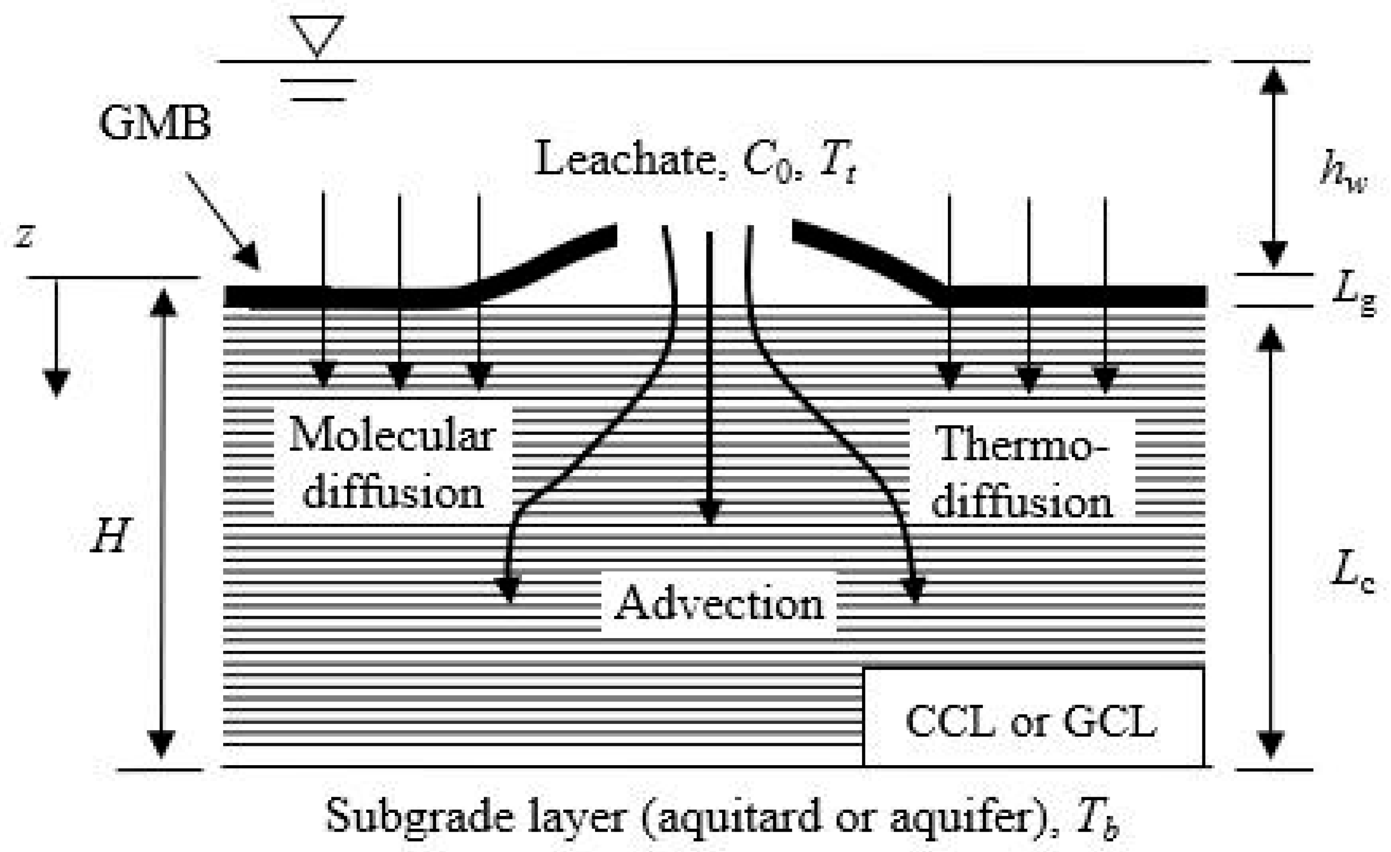
Figure 1 presents the configuration of the composite liner system consisting of two individual layers, i.e., from top to bottom, a geomembrane (GMB) and a clay layer (denoted as CL, which can be either a CCL or a GCL), with an aquitard or aquifer underlying the CL. The CL is assumed to be non-deformable, homogeneous, and fully saturated. The thicknesses of the GMB and CL are $L_g$ and $L_c$, respectively, and the total thickness $H=L_g+L_c$, with the vertical coordinate z directed downward from the top of the GMB. The hydraulic leachate head is $h_w$. The concentration of organic contaminant contained in the leachate is C₀, which is assumed to be sufficiently dilute and could not change the properties of CL [31,32]. Because defects and wrinkles are commonly found in GMBs used for landfill liners, the GMB is assumed to contain wrinkles and defects in this study; consequently, advection plays a role in driving organic contaminant transport in the liner system. The temperature on the top and bottom of the GMB/CL liner system are $T_t$ and $T_b$, respectively, which will produce a temperature gradient and generate contaminant thermodiffusion.

The governing equation for organic contaminant transport through the GMB, considering advection, molecular diffusion, and thermodiffusion, can be expressed as [10,11,24]

$${\displaystyle \frac{\partial C_{\mathrm{g}}(z,t)}{\partial t}}=D_{\mathrm{g}}{\displaystyle \frac{{\partial }^2{C}_{\mathrm{g}}(z,t)}{\partial z^2}}-v_a{\displaystyle \frac{\partial C_{\mathrm{g}}^{\mathrm{hole}}(z,t)}{\partial z}}+{\displaystyle \frac{\partial }{\partial z}}\left(D_{T\mathrm{g}}{\displaystyle \frac{\partial T}{\partial z}}\right)$$

(1)

where $C_{\mathrm{g}}(z,t)$ is the concentration of organic contaminant in the GMB; $D_g$ is the effective diffusion coefficient of organic contaminant in the GMB; $v_a$ is Darcy velocity of the leakage flow through the composite liner; T is the temperature; $D_{T\mathrm{g}}$ is the thermodiffusion coefficient of organic contaminant in the GMB, and $D_{T\mathrm{g}}=C_{\mathrm{g}}(z,t)S_T{D}_{\mathrm{g}}$; $S_T$ is the Soret coefficient, which is defined as the ratio of the thermodiffusion coefficient to the molecular diffusion coefficient [24]; $D_g$ is the effective diffusion coefficient of organic contaminant in the GMB; $C_{\mathrm{g}}^{\mathrm{hole}}(z,t)$ is the concentration of organic contaminant in the flow through the holes in GMB, and $C_{\mathrm{g}}^{\mathrm{hole}}(z,t)=C_{\mathrm{g}}(z,t)/K_{\mathrm{g}}$ [10]; and $K_g$ is the partition coefficient for the organic contaminant and GMB. According to Park and Nibras [33], the sorption between organic contaminant and GMB can be assumed to follow a linear, equilibrium sorption isotherm for low concentrations (<100 mg/L). According to Rowe et al. [34], the $D_g$ and $K_g$ are changed with different temperatures, and can be obtained by

$$D_{\mathrm{g}}=D_{\mathrm{g}}(T_r){\theta }_{d\mathrm{g}}^{(T-T_r)}$$

(2)

$$K_{\mathrm{g}}=K_{\mathrm{g}}(T_r){\theta }_{k\mathrm{g}}^{(T-T_r)}$$

(3)

where $D_g\left(T_r\right)$ and $K_g\left(T_r\right)$ are the effective diffusion coefficient and partition coefficient at a reference temperature $T_r$, respectively; ${\theta }_{\mathit{dg}}$ and ${\theta }_{\mathit{kg}}$ are the constant temperature coefficients for $D_g$ and $K_g$, respectively. The explicit solution to Equation (1) is difficult to obtain because of the variable coefficients. In this study, the $D_g$ and $K_g$ are assumed to be the average value in the GMB for simplified.

Similarly, organic contaminant transport in the CL, considering molecular diffusion, advection, degradation, and thermodiffusion, can be expressed as [10,11,24]

$${\displaystyle \frac{\partial C_{\mathrm{c}}(z,t)}{\partial t}}={\displaystyle \frac{D_{\mathrm{c}}}{R_{d\mathrm{c}}}}{\displaystyle \frac{{\partial }^2{C}_{\mathrm{c}}(z,t)}{\partial z^2}}-{\displaystyle \frac{v_{\mathrm{c}}}{R_{d\mathrm{c}}}}{\displaystyle \frac{\partial C_{\mathrm{c}}(z,t)}{\partial z}}+{\displaystyle \frac{1}{R_{d\mathrm{c}}}}{\displaystyle \frac{\partial }{\partial z}}\left(D_{T\mathrm{c}}{\displaystyle \frac{\partial T}{\partial z}}\right)-\lambda C_{\mathrm{c}}(z,t)$$

(4)

where $C_{\mathrm{c}}(z,t)$ is the contaminant concentration in the CL; $D_c$ is the effective diffusion coefficient of the organic contaminant in the CL; $v_c$ is the seepage velocity in CL and is calculated as $v_c=v_a/n_c$, $n_c$ is the porosity of the CCL; $D_{\mathit{Tc}}$ is the thermodiffusion coefficient of the organic contaminant in the CCL, and $D_{T\mathrm{c}}=C_{\mathrm{c}}(z,t)S_T{D}_{\mathrm{c}}$; $\lambda$ is the first-order degradation constant for dissolved organic contaminant masses in the pore water of CL and is assumed to be calculated as $\lambda = ln\left(2\right)/t_{1/2}$, $t_{1/2}$ is the organic contaminant half-life in CL; and $R_{\mathit{dc}}$ is the retardation factor and can be obtained by

$$R_{d\mathrm{c}}=1+{\displaystyle \frac{{\rho }_{d\mathrm{c}}{K}_{d\mathrm{c}}}{n_{\mathrm{c}}}}$$

(5)

where ${\rho }_{\mathit{dc}}$ and $K_{\mathit{dc}}$ are, respectively, the dry density and distribution coefficient of the CL. The effective diffusion coefficient $D_c$ and distribution coefficient $K_{\mathit{dc}}$ are reported to change with different temperatures [7,35], which are neglected in this study for simplicity, and this is the limitation of the proposed analytical model.

One-dimensional heat conduction in the GMB/CL is assumed to be at steady state. Under this assumption, the general solution to the governing equation of one-dimensional heat conduction is

$$T_{\mathrm{g}}=A_{\mathrm{g}}z+B_{\mathrm{g}}$$

(6)

$$T_{\mathrm{c}}=A_{\mathrm{c}}z+B_{\mathrm{c}}$$

(7)

where $T_g$ and $T_c$ are the temperature in the GMB and CL, respectively; $A_g$ and $A_c$ are proportionality constants about the temperature distribution of GMB and CL, respectively; and $B_g$ and $B_c$ are coefficients to be determined by the temperature boundary conditions.

According to Bouazza et al. [36], the heat flux, $Q_T$, in the GMB/CCL composite liner can be expressed as

$$Q_T=-\kappa \nabla T+C_p{v}_a{\rho }_w\left(T-T_r\right)$$

(8)

where $\kappa$ is the thermal conductivity; $\Delta T$ is the temperature gradient; $C_p$ is the specific heat capacity of liquid; ${\rho }_w$ is the density of liquid; and $T_r$ is the reference temperature.

Substituting Equations (6) and (7) into Equations (1) and (4), the governing equation of $C_{\mathrm{g}}(z,t)$ and $C_{\mathrm{c}}(z,t)$ can be reformulated as

$${\displaystyle \frac{\partial C_{\mathrm{g}}(z,t)}{\partial t}}=D_{\mathrm{g}}{\displaystyle \frac{{\partial }^2{C}_{\mathrm{g}}(z,t)}{\partial z^2}}-\left({\displaystyle \frac{v_a}{K_{\mathrm{g}}}}-A_{\mathrm{g}}{S}_T{D}_{\mathrm{g}}\right){\displaystyle \frac{\partial C_{\mathrm{g}}(z,t)}{\partial z}}$$

(9)

$${\displaystyle \frac{\partial C_{\mathrm{c}}(z,t)}{\partial t}}={\displaystyle \frac{D_{\mathrm{c}}}{R_{d\mathrm{c}}}}{\displaystyle \frac{{\partial }^2{C}_{\mathrm{c}}(z,t)}{\partial z^2}}-\left({\displaystyle \frac{v_{\mathrm{c}}}{R_{d\mathrm{c}}}}-{\displaystyle \frac{A_{\mathrm{c}}{S}_T{D}_{\mathrm{c}}}{R_{d\mathrm{c}}}}\right){\displaystyle \frac{\partial C_{\mathrm{c}}(z,t)}{\partial z}}-\lambda C_{\mathrm{c}}(z,t)$$

(10)

The Darcy velocity of the leakage flow through the composite liner $v_a$ can be determined from the leakage rate through the GMB defects. The leakage rate through a single hole in the composite liner is given by [1,37]

$$Q={\displaystyle \frac{2h_w{L}_w}{H}}\left(kb+\sqrt{kl\theta }\right)$$

(11)

where $L_w$ is the length of wrinkle; 2b is the width of wrinkle; $\theta$ is the transmissivity of the interface between GMB and CL; and $k$ is the hydraulic conductivity of CL. $v_a$ can then be obtained by [8,16,38]

$$v_a=m_{h}Q/A_0$$

(12)

where $m_h$ is the number of the defects in GMB per unit area; $A_0$ is the cross-sectional area of the flow.

The leakage rate $Q$ in Equation (11) adopts the analytical solution developed by Rowe [1] to predict the leakage rate of leachate flow through a single hole of GMB coincident with a wrinkle. This leakage solution agrees well with the results of numerical analysis [37], and has been widely used by researchers to evaluate contaminant transport in liner systems [10,28,29]. According to El-Zein and Rowe [39], one-dimensional predictions of leakage and transport can provide reasonable estimates of contamination in most cases. It should be noted that the effect of wrinkles is accounted for through the geometric parameters $L_w$ and 2b in Equation (11), rather than by artificially increasing the number of defects $m_h$ in Equation (12).

The initial concentrations of the contaminant in GMB and CL are assumed to be $h_{\mathrm{g}}(z)$ and $h_{\mathrm{c}}(z)$, respectively, and therefore, the initial condition of the GMB and CL can be given as

$$C_{\mathrm{g}}(z,t=0)=h_{\mathrm{g}}(z)$$

(13)

$$C_{\mathrm{c}}(z,t=0)=h_c(z)$$

(14)

The top boundary condition for the GMB/CCL composite liner system is [40]:

$${\left.C_{\mathrm{g}}(z,t)\right|}_{z=0}=K_{\mathrm{g}}{C}_0$$

(15)

The continuity conditions in terms of the contaminant concentration and mass flux at the interface between GMB and CL are

$${\left.C_{\mathrm{g}}(z,t)\right|}_{z=L_{\mathrm{g}}}={\left.K_{\mathrm{c}}{C}_{\mathrm{c}}(z,t)\right|}_{z=L_{\mathrm{g}}}$$

(16)

$$\begin{array}{l}\left(v_a/K_{\mathrm{g}}-A_{\mathrm{g}}{S}_T{D}_{\mathrm{g}}\right){\left.C_{\mathrm{g}}(z,t)\right|}_{z=L_{\mathrm{g}}}-{\left.D_{\mathrm{g}}{\displaystyle \frac{\partial C_{\mathrm{g}}(z,t)}{\partial z}}\right|}_{z=L_{\mathrm{g}}}=\\ \left(v_{\mathrm{c}}{n}_{\mathrm{c}}-A_{\mathrm{c}}{S}_T{D}_{\mathrm{c}}{n}_{\mathrm{c}}\right){\left.C_{\mathrm{c}}(z,t)\right|}_{z=L_{\mathrm{g}}}-{\left.n_{\mathrm{c}}{D}_{\mathrm{c}}{\displaystyle \frac{\partial C_{\mathrm{c}}(z,t)}{\partial z}}\right|}_{z=L_{\mathrm{g}}}\end{array}$$

(17)

where K_c is the partition coefficient between GMB and CCL.

Two different bottom boundary conditions are considered: (1) a zero-concentration boundary (ZC), and (2) a zero-concentration-gradient (ZCG) boundary, expressed, respectively, as

$${\left.C_{\mathrm{c}}(z,t)\right|}_{z=H}=0$$

(18)

$${\left.{\displaystyle \frac{\partial C_{\mathrm{c}}(z,t)}{\partial z}}\right|}_{z=H}=0$$

(19)

The ZC and ZCG conditions bracket the range of possible subgrade conditions [10,11]. The ZC condition corresponds to a highly permeable subgrade (e.g., an active aquifer), providing an upper-bound estimate of contaminant flux, while the ZCG condition corresponds to a low-permeability subgrade (e.g., bedrock or an aquitard), providing a lower-bound estimate. The choice between them for practical applications should be guided by site-specific hydrogeological conditions. Mixed or transition boundaries, though potentially more refined, are not considered, as they would significantly complicate the analytical solution.

3. Analytical Solutions

3.1. Steady-State Analytical Solutions

Separating $C_{\mathrm{g}}(z,t)$ and $C_{\mathrm{c}}(z,t)$ into two parts:

$$C_{\mathrm{g}}(z,t)=w_{\mathrm{g}}(z,t)+u_{\mathrm{g}}(z)$$

(20)

$$C_{\mathrm{c}}(z,t)=w_{\mathrm{c}}(z,t)+u_{\mathrm{c}}(z)$$

(21)

Substituting Equations (20) and (21) into Equations (9) and (10), respectively, leads to the governing equation and boundary conditions of $u_{\mathrm{g}}(z)$ and $u_{\mathrm{c}}(z)$. The $u_{\mathrm{g}}(z)$ and $u_{\mathrm{c}}(z)$ are the steady-state concentrations for GMB and CL, respectively, and are determined by the following equation:

$$D_{\mathrm{g}}{\displaystyle \frac{{\partial }^2{u}_{\mathrm{g}}(z)}{\partial z^2}}-\left({\displaystyle \frac{v_a}{K_{\mathrm{g}}}}-A_{\mathrm{g}}{S}_T{D}_{\mathrm{g}}\right){\displaystyle \frac{\partial u_{\mathrm{g}}(z)}{\partial z}}=0$$

(22)

$${\displaystyle \frac{D_{\mathrm{c}}}{R_{d\mathrm{c}}}}{\displaystyle \frac{{\partial }^2{u}_{\mathrm{c}}(z)}{\partial z^2}}-\left({\displaystyle \frac{v_{\mathrm{c}}}{R_{d\mathrm{c}}}}-{\displaystyle \frac{A_{\mathrm{c}}{S}_T{D}_{\mathrm{c}}}{R_{d\mathrm{c}}}}\right){\displaystyle \frac{\partial u_{\mathrm{c}}(z)}{\partial z}}-\lambda u_{\mathrm{c}}(z)=0$$

(23)

The top boundary condition for Equations (22) and (23) is

$${\left.u_{\mathrm{g}}(z)\right|}_{z=0}=K_{\mathrm{g}}{C}_0$$

(24)

The continuity conditions at the interface between GMB and CL are

$${\left.u_{\mathrm{g}}(z)\right|}_{z=L_{\mathrm{g}}}=K_{\mathrm{c}}{\left.u_{\mathrm{c}}(z)\right|}_{z=L_{\mathrm{g}}}$$

(25)

$$\begin{array}{l}{\left.\left(v_a/K_{\mathrm{g}}-A_{\mathrm{g}}{S}_T{D}_{\mathrm{g}}\right)u_{\mathrm{g}}(z)\right|}_{z=L_{\mathrm{g}}}-{\left.D_{\mathrm{g}}{\displaystyle \frac{\partial u_{\mathrm{g}}(z)}{\partial z}}\right|}_{z=L_{\mathrm{g}}}\\ ={\left.\left(v_{\mathrm{c}}{n}_{\mathrm{c}}-A_{\mathrm{c}}{S}_T{n}_{\mathrm{c}}{D}_{\mathrm{c}}\right)u_{\mathrm{c}}(z)\right|}_{z=L_{\mathrm{g}}}-{\left.n_{\mathrm{c}}{D}_{\mathrm{c}}{\displaystyle \frac{\partial u_{\mathrm{c}}(z)}{\partial z}}\right|}_{z=L_{\mathrm{g}}}\end{array}$$

(26)

The bottom boundary conditions for Equations (22) and (23) are

$${\left.u_{\mathrm{c}}(z)\right|}_{z=H}=0$$

(27)

$${\left.{\displaystyle \frac{\partial u_{\mathrm{c}}(z)}{\partial z}}\right|}_{z=H}=0$$

(28)

The general solution to Equations (22) and (23) are

$$u_{\mathrm{g}}(z)=E_1\exp \left[{\displaystyle \frac{v_a-A_{\mathrm{g}}{S}_T{D}_{\mathrm{g}}{K}_{\mathrm{g}}}{D_{\mathrm{g}}{K}_{\mathrm{g}}}}z\right]+F_1$$

(29)

$$u_{\mathrm{c}}(z)=E_2\exp (r_{1}z)+F_2\exp (r_{2}z)$$

(30)

where E₁ to F₂ are coefficients that can be obtained by substituting Equations (29) and (30) into Equations (24) to (26) and Equation (27) or Equation (28); $r_1$ and $r_2$ are determined by

$$r_{1,2}={\displaystyle \frac{(v_{\mathrm{c}}-A_{\mathrm{c}}{S}_T{D}_{\mathrm{c}})\pm \sqrt{{(v_{\mathrm{c}}-A_{\mathrm{c}}{S}_T{D}_{\mathrm{c}})}^2+4{\lambda }_{\mathrm{c}}{D}_{\mathrm{c}}{R}_{d\mathrm{c}}}}{2D_{\mathrm{c}}}}$$

(31)

The steady-state mass flux, $J_{ss}$, at the bottom boundary can be obtained as follows:

$$J_{ss}=\left\{\begin{array}{l}-n_c{D}_c\left(E_2{r}_1\exp (r_{1}H)+F_2{r}_2\exp (r_{2}H)\right) \mathrm{for} \mathrm{ZC} \mathrm{boundary} \mathrm{condition}\\ \left(v_a-A{S}_T{n}_{\mathrm{c}}{D}_{\mathrm{c}}\right)\left(E_2\exp (r_{1}H)+F_2\exp (r_{2}H)\right) \mathrm{for} \mathrm{ZCG} \mathrm{boundary} \mathrm{condition}\end{array}\right.$$

(32)

where “ZC” and “ZCG” represent the zero-concentration bottom boundary and zero-concentration-gradient bottom boundary, respectively.

3.2. Fully Transient Analytical Solutions

Substituting Equations (20) and (21) into Equations (9) and (10), respectively, leads to the governing equation of $w_{\mathrm{g}}(z,t)$ and $w_{\mathrm{c}}(z,t)$:

$${\displaystyle \frac{\partial w_{\mathrm{g}}(z,t)}{\partial t}}=D_{\mathrm{g}}{\displaystyle \frac{{\partial }^2{w}_{\mathrm{g}}(z,t)}{\partial z^2}}-\left({\displaystyle \frac{v_a}{K_{\mathrm{g}}}}-A_{\mathrm{g}}{S}_T{D}_{\mathrm{g}}\right){\displaystyle \frac{\partial w_{\mathrm{g}}(z,t)}{\partial z}}$$

(33)

$${\displaystyle \frac{\partial w_{\mathrm{c}}(z,t)}{\partial t}}={\displaystyle \frac{D_{\mathrm{c}}}{R_{d\mathrm{c}}}}{\displaystyle \frac{{\partial }^2{w}_{\mathrm{c}}(z,t)}{\partial z^2}}-\left({\displaystyle \frac{v_{\mathrm{c}}}{R_{d\mathrm{c}}}}-{\displaystyle \frac{A_{\mathrm{c}}{S}_T{D}_{\mathrm{c}}}{R_{d\mathrm{c}}}}\right){\displaystyle \frac{\partial w_{\mathrm{c}}(z,t)}{\partial z}}-\lambda w_{\mathrm{c}}$$

(34)

Similarly, substituting Equations (24) to (28) into Equations (15) to (19), respectively, leads to the boundary conditions and continuity conditions of $w_{\mathrm{g}}(z,t)$ and $w_{\mathrm{c}}(z,t)$:

$${\left.w_{\mathrm{g}}(z,t)\right|}_{z=0}=0$$

(35)

$${\left.w_{\mathrm{g}}(z,t)\right|}_{z=L_{\mathrm{g}}}=K_{\mathrm{c}}{\left.w_{\mathrm{c}}(z,t)\right|}_{z=L_{\mathrm{g}}}$$

(36)

$$\begin{array}{l}{\left.\left(v_a/K_{\mathrm{g}}-A_{\mathrm{g}}{S}_T{D}_{\mathrm{g}}\right)w_{\mathrm{g}}(z,t)\right|}_{z=L_{\mathrm{g}}}-{\left.D_{\mathrm{g}}{\displaystyle \frac{\partial w_{\mathrm{g}}(z,t)}{\partial z}}\right|}_{z=L_{\mathrm{g}}}\\ ={\left.\left(v_{\mathrm{c}}{n}_{\mathrm{c}}-A_{\mathrm{c}}{S}_T{n}_{\mathrm{c}}{D}_{\mathrm{c}}\right)w_{\mathrm{c}}(z,t)\right|}_{z=L_{\mathrm{g}}}-{\left.n_{\mathrm{c}}{D}_{\mathrm{c}}{\displaystyle \frac{\partial w_{\mathrm{c}}(z,t)}{\partial z}}\right|}_{z=L_{\mathrm{g}}}\end{array}$$

(37)

$${\left.w_{\mathrm{c}}(z,t)\right|}_{z=H}=0$$

(38)

and

$${\left.{\displaystyle \frac{\partial w_{\mathrm{c}}(z,t)}{\partial z}}\right|}_{z=H}=0$$

(39)

The initial conditions of Equations (33) and (34) can be obtained by substituting Equations (20) and (21) into Equations (13) and (14), respectively, and can be expressed as follows:

$$w_{\mathrm{g}}(z,0)=h_{\mathrm{g}}(z)-u_{\mathrm{g}}(z)$$

(40)

$$w_{\mathrm{c}}(z,0)=h_{\mathrm{c}}(z)-u_{\mathrm{c}}(z)$$

(41)

Based on the conditions and assumptions discussed above, the analytical solutions are derived to solve Equations (33) and (34) (see Appendix A). The analytical solutions to the governing Equations (33) and (34) are given as follows:

$$w_{\mathrm{g}}(z,t)={\displaystyle \sum _{k=1}^{\infty }{S}_k{f}_{k,\mathrm{g}}(z)\exp (a_{\mathrm{g}}z-{\delta }_{k}t)}$$

(42)

$$w_{\mathrm{c}}(z,t)={\displaystyle \sum _{k=1}^{\infty }{S}_k{f}_{k,\mathrm{c}}(z)\exp (a_{\mathrm{c}}z-{\delta }_{k}t)}$$

(43)

where

$$a_{\mathrm{g}}={\displaystyle \frac{v_a-A_{\mathrm{g}}{S}_T{D}_{\mathrm{g}}{K}_{\mathrm{g}}}{2D_{\mathrm{g}}{K}_{\mathrm{g}}}}, a_c={\displaystyle \frac{v_c-A_{\mathrm{c}}{S}_T{D}_{\mathrm{c}}}{2D_{\mathrm{c}}}}$$

(44)

$$f_{k,\mathrm{g}}(z)=\left\{\begin{array}{l}{H}_k\sin \left({\xi }_{k,\mathrm{g}}z\right) \mathrm{when} {\delta }_k\ge {\displaystyle \frac{{\left(v_a-A_{\mathrm{g}}{S}_T{D}_{\mathrm{g}}{K}_{\mathrm{g}}\right)}^2}{4D_{\mathrm{g}}{K}_{\mathrm{g}}^2}}\\ H_k\sinh \left({\xi }_{k,\mathrm{g}}z\right) \mathrm{when} {\delta }_k<{\displaystyle \frac{{\left(v_a-A_{\mathrm{g}}{S}_T{D}_{\mathrm{g}}{K}_{\mathrm{g}}\right)}^2}{4D_{\mathrm{g}}{K}_{\mathrm{g}}^2}} \end{array}\right.$$

(45)

$$f_{k,\mathrm{c}}(z)=\left\{\begin{array}{l}{G}_k\sin \left({\xi }_{k,\mathrm{c}}z\right)+Q_k\cos \left({\xi }_{k,\mathrm{c}}z\right) \mathrm{when} {\delta }_k\ge {\displaystyle \frac{{\left(v_{\mathrm{c}}-A_{\mathrm{c}}{S}_T{D}_{\mathrm{c}}\right)}^2}{4D_{\mathrm{c}}{R}_{d\mathrm{c}}}}+\lambda \\ G_k\sinh \left({\xi }_{k,\mathrm{c}}z\right)+Q_k\cosh \left({\xi }_{k,\mathrm{c}}z\right) \mathrm{when} {\delta }_k<{\displaystyle \frac{{\left(v_{\mathrm{c}}-A_{\mathrm{c}}{S}_T{D}_{\mathrm{c}}\right)}^2}{4D_{\mathrm{c}}{R}_{d\mathrm{c}}}}+\lambda \end{array}\right.$$

(46)

$${\xi }_{k,\mathrm{g}}=\sqrt{\left|{\displaystyle \frac{{\delta }_k}{D_{\mathrm{g}}}}-a_{\mathrm{g}}^2\right|}, {\xi }_{k,\mathrm{c}}=\sqrt{\left|{\displaystyle \frac{R_{d\mathrm{c}}{\delta }_k}{D_{\mathrm{c}}}}-a_{\mathrm{c}}^2-{\displaystyle \frac{R_{d\mathrm{c}}\lambda }{D_{\mathrm{c}}}}\right|}$$

(47)

$$H_k={\displaystyle \frac{N_{3k}{N}_{7k}-N_{8k}{N}_{2k}}{N_{1k}{N}_{7k}}}{Q}_k$$

(48)

$$G_k=-{\displaystyle \frac{N_{8k}}{N_{7k}}}Qk$$

(49)

$$S_k={\displaystyle \frac{{\displaystyle {\int }_0^{L_{\mathrm{g}}}\left[h_{\mathrm{g}}(z)-u_{\mathrm{g}}(z)\right]f_{k,\mathrm{g}}(z)\exp (-a_{\mathrm{g}}z)\mathrm{d}z}+n_{\mathrm{c}}{R}_{d\mathrm{c}}\eta K_{\mathrm{c}}{\displaystyle {\int }_{L_{\mathrm{g}}}^H\left[h_{\mathrm{c}}(z)-u_{\mathrm{c}}(z)\right]f_{k,\mathrm{c}}(z)\exp (-a_{\mathrm{c}}z)\mathrm{d}z}}{{\displaystyle {\int }_0^{L_{\mathrm{g}}}{f}_{k,\mathrm{g}}^2(z)\mathrm{d}z+}{n}_{\mathrm{c}}{R}_{d\mathrm{c}}\eta K_{\mathrm{c}}{\displaystyle {\int }_{L_{\mathrm{g}}}^H{f}_{k,\mathrm{c}}^2(z)\mathrm{d}z}}}$$

(50)

The values of ${\delta }_k$ can be obtained by the following equation:

$$N_{7k}\left(N_{1k}{N}_{6k}-N_{3k}{N}_{4k}\right)+N_{8k}\left(N_{2k}{N}_{4k}-N_{1k}{N}_{5k}\right)=0$$

(51)

where the expressions of N_1k to N_8k are given in Appendix A.

The fully transient analytical solution to the governing Equation (1) can be obtained by substituting Equations (30) and (43) into Equation (21) as follows:

$$C_{\mathrm{g}}(z,t)=E_1\exp \left[{\displaystyle \frac{v_a-A_{\mathrm{g}}{S}_T{D}_{\mathrm{g}}{K}_{\mathrm{g}}}{D_{\mathrm{g}}{K}_{\mathrm{g}}}}z\right]+F_1+{\displaystyle \sum _{k=1}^{\infty }{S}_k{f}_{k,\mathrm{g}}(z)\exp (a_{\mathrm{g}}z-{\delta }_{k}t)}$$

(52)

Similarly, the fully transient analytical solution to the governing Equation (4) can be obtained by substituting Equations (30) and (43) into Equation (21) as follows:

$$C_{\mathrm{c}}(z,t)=E_2\exp (r_{1}z)+F_2\exp (r_{2}z)+{\displaystyle \sum _{k=1}^{\infty }{S}_k{f}_{k,\mathrm{c}}(z)\exp (a_{\mathrm{c}}z-{\delta }_{k}t)}$$

(53)

The contaminant mass flux, $J$, at the base of the liner can be obtained as

$${\left.J(z,t)\right|}_{z=H}=\left(v_a-A_{\mathrm{c}}{S}_T{n}_{\mathrm{c}}{D}_{\mathrm{c}}\right){\left.C_{\mathrm{c}}(z,t)\right|}_{z=H}-n_{\mathrm{c}}{D}_{\mathrm{c}}{\left.{\displaystyle \frac{\partial C_{\mathrm{c}}(z,t)}{\partial z}}\right|}_{z=H}$$

(54)

The cumulative mass outflow, $M$, at the base of the liner can be obtained as

$${\left.M(z,t)\right|}_{z=H}=\left(v_a-A_{\mathrm{c}}{S}_T{n}_{\mathrm{c}}{D}_{\mathrm{c}}\right){\displaystyle {\int }_0^t{\left.C_{\mathrm{c}}(z,\tau )\right|}_{z=H} \mathrm{d}\tau }-n_{\mathrm{c}}{D}_{\mathrm{c}}{\displaystyle {\int }_0^t{\left.\frac{\partial C_{\mathrm{c}}(z,\tau )}{\partial z}\right|}_{z=H}\mathrm{d}\tau }$$

(55)

The infinite series in Equations (53) and (54) converges quickly, with errors smaller than 1%, 0.1%, and 0.01% when summing 5 terms, 10 terms, and 15 terms, respectively.

4. Model Verification

4.1. Comparisons with Experimental Results

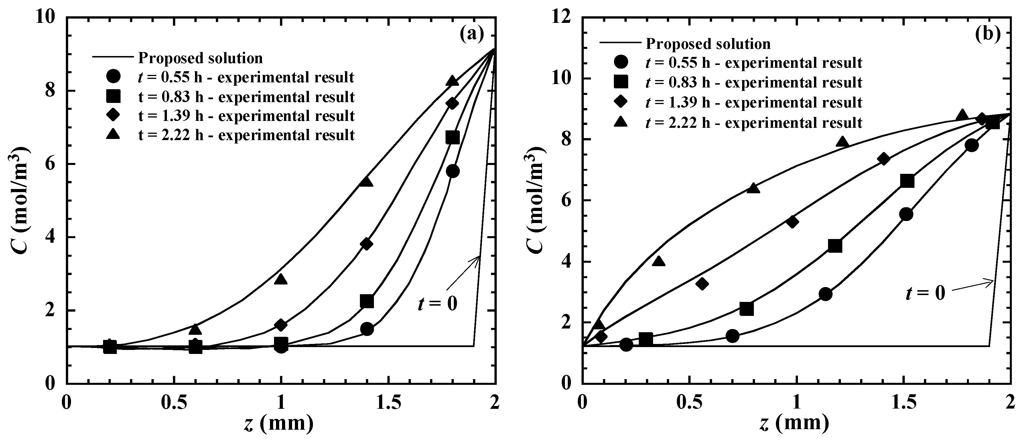
Two thermodiffusion experiments in compact clays reported by Rosanne et al. [23] are used to validate the proposed analytical solution. Both experiments describe the transport of NaCl solution in a 2 mm thick compact clay with porosity n = 0.6. Although the present study focuses on organic contaminants, the proposed solution can also be used to analyze the transport of inorganic compounds. For experiment 1, the concentrations of NaCl solution on the top and bottom boundaries were 1.01 mol/m³ ($C_t$) and 9.14 mol/m³ ($C_b$), respectively, and the temperatures on the top and bottom boundaries were 311 K ($T_t$) and 285.1 K ($T_b$), respectively. For experiment 2, the values of $C_t$, $C_b$, $T_t$ and $T_b$ are 1.21 mol/m³, 8.83 mol/m³, 284.8 K and 311.1 K, respectively. According to Rosanne et al. [23], the effective diffusion coefficient of the compact clay for experiments 1 and 2 was 1.7 × 10⁻¹¹ m²/s and 6 × 10⁻¹¹ m²/s, respectively; these values were measured in pure diffusion tests without any thermal gradient. The Soret coefficients for experiments 1 and 2 were determined by inverse analysis using the measured concentration profile at t = 0.55 h from the thermodiffusion experiments of Rosanne et al. [23], yielding values of −0.26 and 0.21 K⁻¹, respectively. These values were not taken directly from Rosanne et al. [23], because their reported Soret coefficients were obtained under a numerical model with temperature-dependent diffusion coefficients, whereas the present analytical solution assumes constant coefficients evaluated at the average temperature. The same S_T values were then used to predict the concentration profiles at subsequent times (t = 0.83, 1.39, and 2.22 h) without further adjustment.

The proposed analytical model does not consider a non-zero concentration at the bottom boundary; therefore, the boundary conditions are modified accordingly.

$$C_{\mathrm{c}}(0,t)=C_t$$

(56)

$$C_{\mathrm{c}}(H,t)=C_b$$

(57)

Based on the proposed analytical model, the analytical solution for the CCL is given as follows:

$$C_c(z,t)=E\exp (r_{1}z)+F\exp (r_{2}z)-{\displaystyle \sum _{k=0}^{\infty }{S}_k\sin \left(\frac{k\pi z}{H}\right)\exp \left(a_{c}z-{\delta }_{k}t\right)}$$

(58)

where

$$S_k={\displaystyle \frac{{\displaystyle {\int }_0^H\left[h_{\mathrm{c}}(z)-E\exp (r_{1}z)-F\exp (r_{2}z)\right]\sin \left(\frac{k\pi z}{H}\right)\exp \left(-a_{c}z\right)\mathrm{d}z}}{{\displaystyle {\int }_0^H{\sin }^2\left(\frac{k\pi z}{H}\right)\mathrm{d}z}}}$$

(59)

$$E+F=C_t$$

(60)

$$E\exp (r_{1}H)+F\exp (r_{2}H)=C_b$$

(61)

$${\delta }_k={\displaystyle \frac{D_c}{R_{dc}}}{\displaystyle \frac{k^2{\pi }^2}{H^2}}+{\displaystyle \frac{D_c{a}_{\mathrm{c}}^2}{R_{dc}}}+{\lambda }_c$$

(62)

Figure 2 compares the sodium chloride concentration profiles within the compact clay obtained from the proposed analytical solution with the experimental results of Rosanne et al. [23] at t = 0.55, 0.83, 1.39 and 2.22 h. To quantitatively evaluate the agreement, the root mean square error (RMSE) and coefficient of determination (R²) were calculated for each time instant as well as for the overall dataset. The results are summarized in

Table 1. Quantitative comparison between the proposed analytical solution and experimental data of Rosanne et al. [23].

Time t (h)	Experiment 1		Experiment 2
	RMSE (mol/m3)	R2	RMSE (mol/m3)	R2
0.55	0.01507	0.99995	0.02247	0.99988
0.83	0.01478	0.99995	0.01023	0.99988
1.39	0.00777	0.99999	0.00845	0.99999
2.22	0.00344	0.99999	0.26210	0.98782
Overall	0.01138	0.99997	0.13172	0.99633

, which confirms the excellent agreement between the proposed analytical solution and the experimental data.

4.2. Comparisons with an Analytical Solution

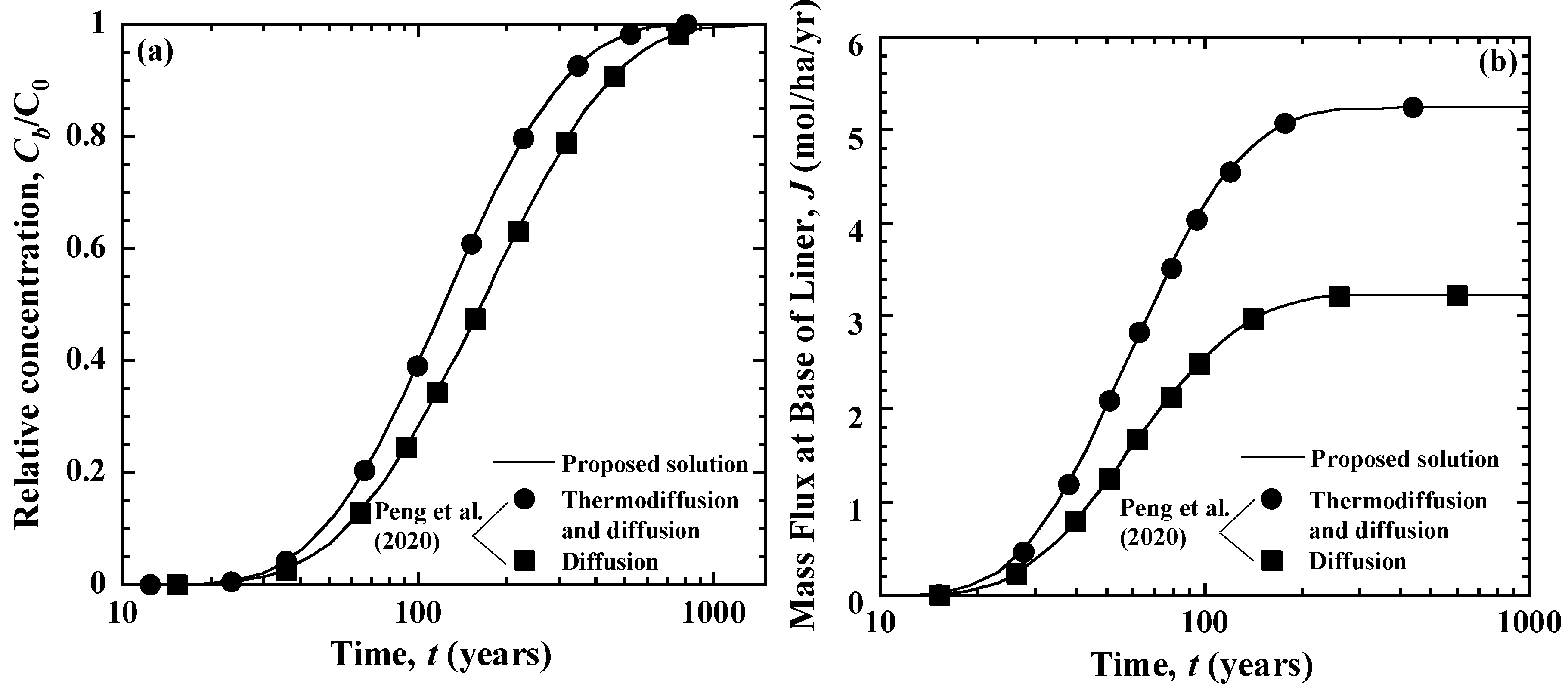
In this section, a closed-form analytical solution for degradable organic contaminant transport through GMB/CCL composite liners presented by Peng et al. [26] is used to validate the proposed analytical solution. A hypothetical GMB/CCL composite liner system suggested by Peng et al. [26] is adopted here. The related parameters were given in Table 1 in Peng et al. [26]. The solution of Peng et al. [26] does not consider the defects and wrinkles occurred in GMB, so the seepage velocity is assumed to be zero in this section. The comparisons between the proposed analytical solution and the solution of Peng et al. [26] are presented in Figure 3, including (a) contaminant concentration at the base of the liner for the ZCG boundary condition, and (b) contaminant mass flux at the base of the liner for the ZC boundary condition. Two kinds of simulation were conducted with and without the effect of thermodiffusion. Figure 3 indicates that, for both boundary conditions, the proposed analytical solution is in excellent agreement with the analytical solution of Peng et al. [26].

4.3. Comparisons with a Numerical Model

To more comprehensively verify the proposed analytical solution, the contaminant mass flux profiles for the GMB/CCL and GMB/GCL composite liner systems calculated by the analytical solution are compared with those obtained from the finite-element software COMSOL Multiphysics 5.4. Benzene, a common organic contaminant in landfill leachates [41], is chosen as the representative contaminant. The leachate is assumed to contain a constant benzene concentration of 100 $\mathsf{\mu }\mathrm{g}/\mathrm{L}$ [42]. The transport properties of Benzene for the GMB/CCL and GMB/GCL composite liner systems are presented in

Table 2. Benzene transport parameters for the GMB/CCL and GMB/GCL composite liner systems.

Property	GMB	CCL	GCL
Thickness (m)	0.0015 [13,14]	1 [13,14]	0.01 [13,14]
Effective diffusion coefficient at $T_r$, D (×10−13 m2/s)	2.7 [34]	6000 [13,14]	3850 [43]
Partition coefficient at $T_r$	36 [34]	36 [34]	36 [34]
Distribution coefficient at $T_r$, $K_d$ (mL/g)	-	0.5 [13,14]	4.4 [43]
Porosity	-	0.4 [44,45]	0.8 [46,47]
Dry density, ${\rho }_d$ (kg/m3)	-	1650 [13,14]	440 [13,14]
Thermal conductivity, $\kappa$ (W/mK)	0.3 [48,49]	1.2 [26]	0.7 [36]
Hydraulic conductivity, k (×10−9 m/s)	-	1 [10,11]	0.01 [13,14]
Length of the wrinkle, $L_w$ (m)	200 [50,51]	-	-
Width of the wrinkle, 2b (m)	0.2 [50]	-	-
Number of defects in GMB per unit area, $m_h$ (holes/ha)	2.5 [52]	-	-
Hydraulic leachate head, $h_w$ (m)	0.3 [10,11]
Interface transmissivity, $\theta$ (×10−8 m2/s)	5 [10,11]
Half-life of benzene, $t_{1/2}$ (years)	20 [53]
The temperature on the top of the liner, $T_t$ (K)	324.15 [7,54]
The temperature on the top of the liner, $T_t$ (K)	284.15 [55,56]
The reference temperature, $T_r$ (K)	295.15
Soret coefficient, $S_T$ (K−1)	0.01 [23,57]

. The constant temperature coefficients ${\theta }_{\mathit{dg}}$ and ${\theta }_{\mathit{kg}}$ are 1.083 and 1.026, respectively [34].

In the COMSOL model, the GMB and CCL layers in the GMB/CCL system were discretized with 3 and 200 elements, respectively, while the GMB and GCL layers in the GMB/GCL system were discretized with 5 and 30 elements, respectively. A mesh refinement study confirmed that further refinement altered the results by less than 0.5%. The automatic Newton solver was used to solve the nonlinear system. The top boundary was set to a constant concentration $C_{\mathrm{g}}(0,t)=K_{\mathrm{g}}{C}_0$, and the bottom boundary was assigned as either ZC or ZCG, with flux continuity enforced at the GMB–clay interface.

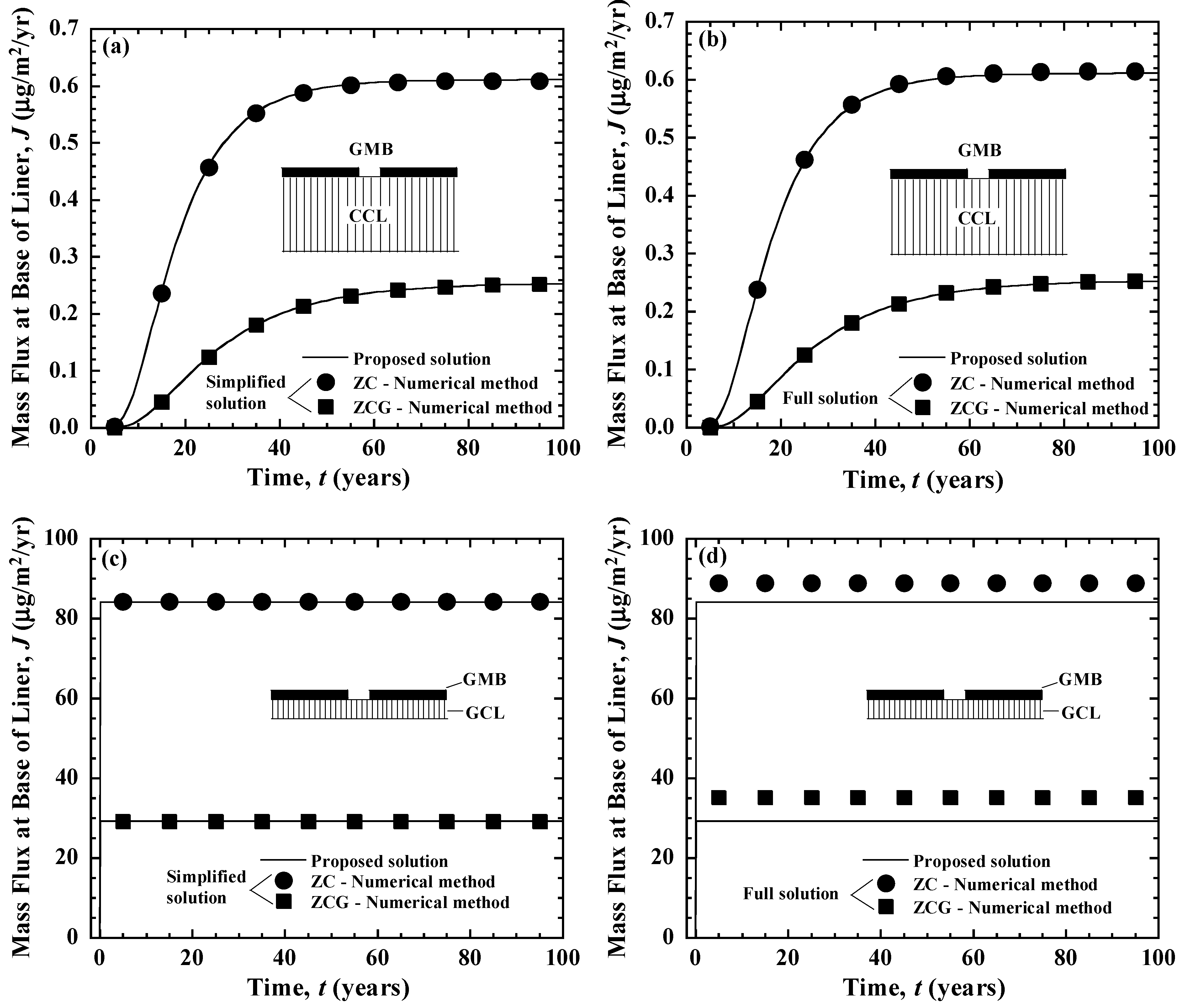
Two kinds of numerical results obtained by the COMSOL Multiphysics 5.4 are compared with the proposed analytical solution, which are presented in Figure 4. Figure 4a,c present the simplified numerical solution with the assumption of constant $D_g$ and $K_g$, and Figure 4b,d present the full numerical solution with temperature-dependent $D_g$ and $K_g$. Figure 4a,c show that, for both ZC and ZCG boundary conditions, the benzene mass flux curves from the proposed analytical solution agree closely with those from the simplified numerical model, confirming the accuracy of the analytical solution. For the GMB/CCL system (Figure 4a), the relative errors $E_r$ between the analytical and numerical solutions are 0.19% and 0.28% for the ZC and ZCG boundary conditions, respectively. For the GMB/GCL system (Figure 4c), the corresponding errors are 0.19% and 0.05%, respectively.

Figure 4b shows that the proposed analytical solution can accurately predict contaminant transport in the GMB/CCL composite liner system even with constant D_g and K_g, yielding relative errors of 0.61% and 0.62% for the ZC and ZCG boundary conditions, respectively. However, Figure 4d shows that the analytical solution predicts slightly lower mass fluxes than the full numerical solution for the GMB/GCL system, with relative errors $E_r$ = 5.4% and 17.3% for ZC and ZCG boundary conditions, respectively. The relative errors in the GMB/GCL system under both the ZC and ZCG conditions (Figure 4d) arise from the analytical simplification that D_g and K_g are assumed constant in the GMB, whereas the numerical solution accounts for their temperature dependence. This simplification introduces negligible error in the GMB/CCL system because the GMB thickness is only 0.15% of the CCL thickness. However, for the GMB/GCL system, the GMB thickness is 15% of the GCL thickness, making the error non-negligible. Overall, the analytical solution is sufficiently accurate for GMB/CCL systems under all conditions. For GMB/GCL systems, it captures the key trends and provides conservative estimates for preliminary design. For a final detailed design requiring high accuracy, the full numerical model with temperature-dependent properties is recommended.

5. Parametric Study

Based on the example in Section 4.3, the verified analytical solutions are used to investigate the effects of thermodiffusion, Soret coefficient, and thermal conductivity on benzene transport through the GMB/CL composite liner systems.

5.1. Effect of Thermodiffusion

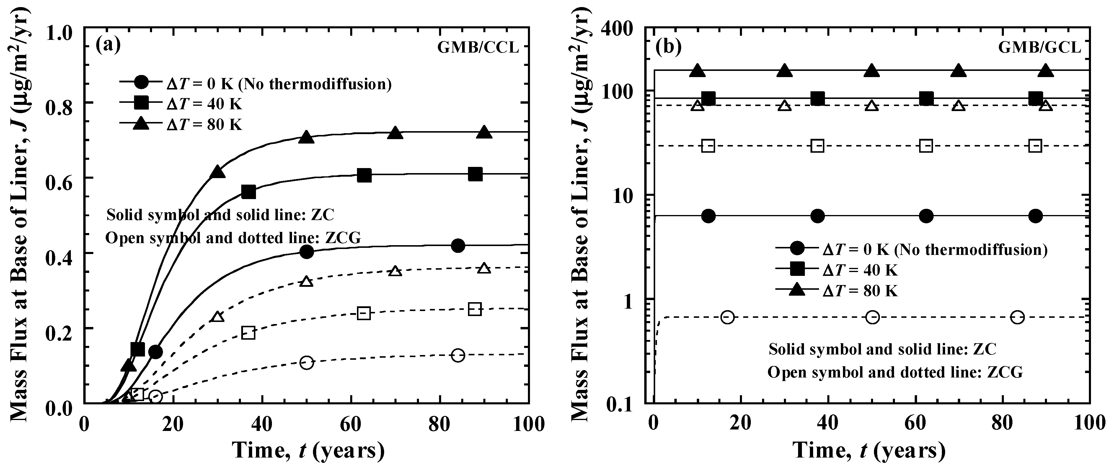
Rowe [7,54] and Rowe and Hoor [19] reported that temperatures on the upper surface of landfill liners can range from 30 to 90 °C, while aquifer temperatures below the liner range from 5 to 25 °C [55,56]. Thus, the temperature difference $\Delta T$ between the top and bottom boundaries can vary from 5 to 85 K. To illustrate the importance of considering thermodiffusion in the analysis of benzene transport through the GMB/CL liner system, Figure 5 presents the benzene mass flux J at the base of the liner for three different $\Delta T$ (=0, 40 and 80 K) under both ZC and ZCG conditions. The bottom temperature is kept constant at 284.15 K in all cases. Figure 5a,b present the J curves for GMB/CCL and GMB/GCL composite liner systems, respectively, and indicate that J increases with increasing ∆T for both boundary conditions. For example, in the GMB/CCL system under the ZC condition, the steady-state mass flux $J_{ss}$ increases from 0.42 to 0.72 µg/m²/year (i.e., 71% increment) when $\Delta T$ increases from 0 to 80 K. The GMB/GCL system exhibits much higher mass fluxes and a stronger temperature response than the GMB/CCL system because of its smaller total thickness. For all three $\Delta T$ values, the ZC boundary condition yields higher J values and shorter breakthrough times than the ZCG condition, because advection is the only mechanism driving contaminant outflow under the ZCG condition.

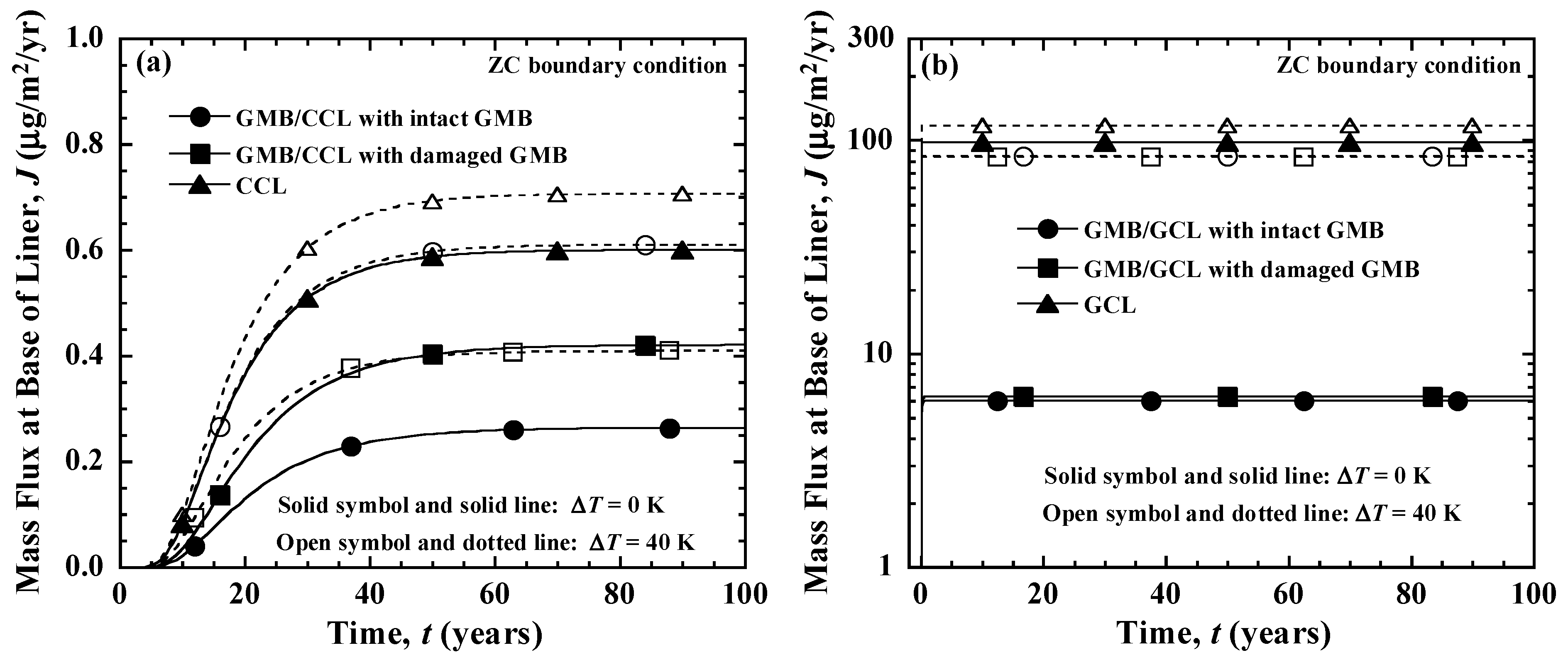
To illustrate the effect of thermodiffusion in the presence of advection, Figure 6 shows the benzene mass flux under the ZC condition for three liner configurations: (i) GMB/CL with a damaged GMB (including defects and wrinkles), (ii) GMB/CL with an intact GMB, and (iii) CL alone (representing a heavily damaged or missing GMB). As expected, the mass fluxes increase significantly when the GMB is damaged or absent because advection becomes more dominant. For $\Delta T$ = 40 K, $J_{ss}$ increases from 6.01 µg/m²/year for the GMB/GCL system to 117.16 µg/m²/year for the GCL alone. Figure 6a shows that when $\Delta T$ increases from 0 to 40 K, $J_{ss}$ increases by 57.7% for the intact GMB/CCL system, by 45.2% for the damaged GMB/CCL system, and by only 18.3% for the CCL alone. Thus, the relative effect of thermodiffusion decreases as advection becomes more important. Similar trends are observed in Figure 6b for GCL-based systems.

5.2. Effect of Soret Coefficient

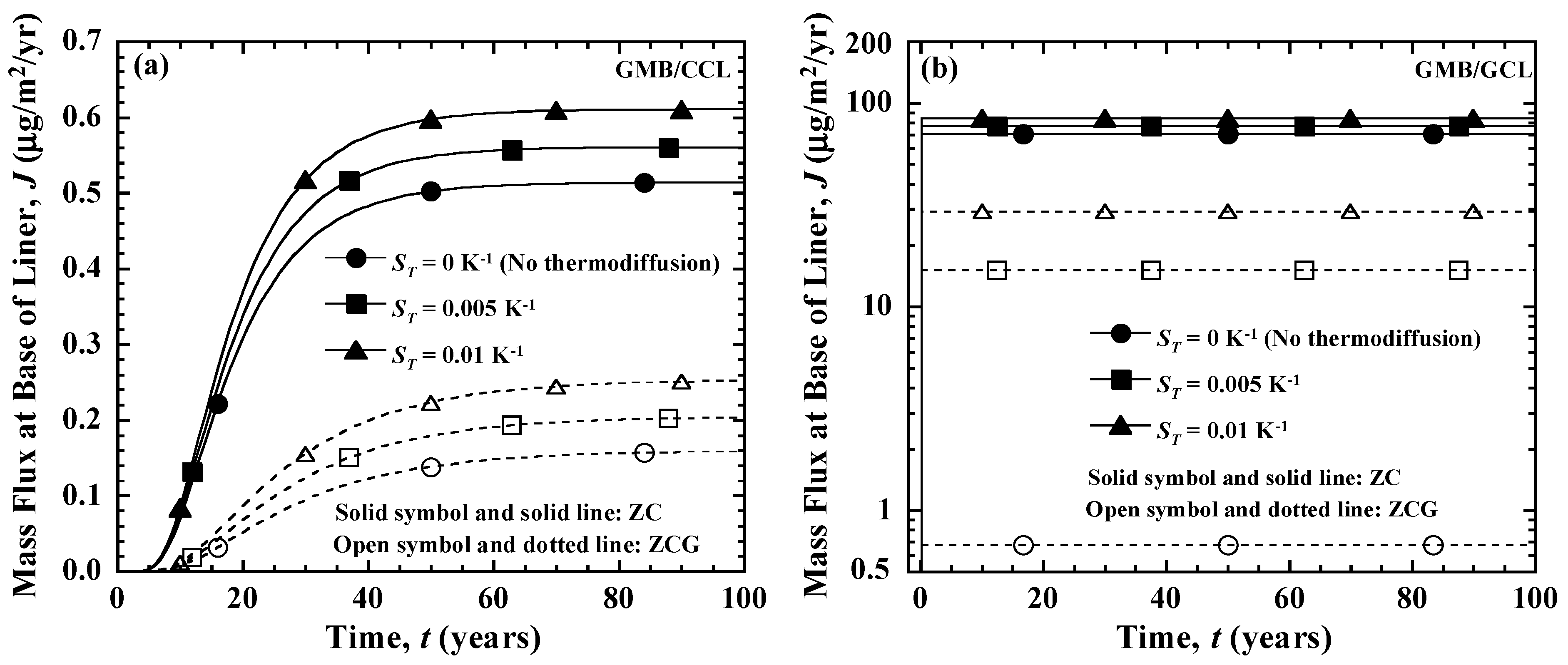
The Soret coefficient S_T has been reported to range from 0.005 to 0.05 K⁻¹ [23,57]. To illustrate the effect of the Soret coefficient on benzene transport through the GMB/CL liner system, Figure 7 presents the benzene mass flux J at the base of the liner for three different Soret coefficients $S_T$ (= 0, 0.005, and 0.01 K⁻¹). Figure 7a,b present the J curves for GMB/CCL and GMB/GCL composite liner systems, respectively, and indicate that J increases almost linearly with increasing $S_T$ for both ZC and ZCG boundary conditions.

Table 3. Steady-state mass flux $J_{ss}$ for GMB/CCL and GMB/GCL composite liner system for different S_T.

${\mathit{S}}_{\mathit{T}}$ (K−1)	Steady-State Mass Flux ${\mathit{J}}_{\mathbf{s}\mathbf{s}}$ (µg/m2/year)
	GMB/CCL Composite Liner System		GMB/GCL Composite Liner System
	ZC Condition	ZCG Condition	ZC Condition	ZCG Condition
0	0.514	0.159	70.370	0.680
0.005	0.560 (8.9% ↑)	0.204 (28.3% ↑)	77.010 (9.4% ↑)	14.978 (2102% ↑)
0.01	0.610 (8.9% ↑)	0.252 (23.5% ↑)	84.025 (9.1% ↑)	29.137 (94.5% ↑)

presents the values of $J_{ss}$ for GMB/CCL and GMB/GCL composite liner system for the three different $S_T$. The ZCG boundary condition shows a higher relative increase in $J_{ss}$ than the ZC condition as S_T increases, because thermodiffusion significantly raises the benzene concentration in the liner, which in turn enhances advective mass flux. For $S_T$ = 0 and ZCG condition, the GMB/GCL system gives $J_{ss}$ of the same order as the GMB/CCL system, indicating that even a thin GCL can effectively contain contaminants when advection is the dominant transport mechanism. Under the ZC condition, however, the GMB/GCL system exhibits a steady-state mass flux two orders of magnitude higher than that of the GMB/CCL system, because diffusion becomes much more important.

5.3. Effect of Thermal Conductivity

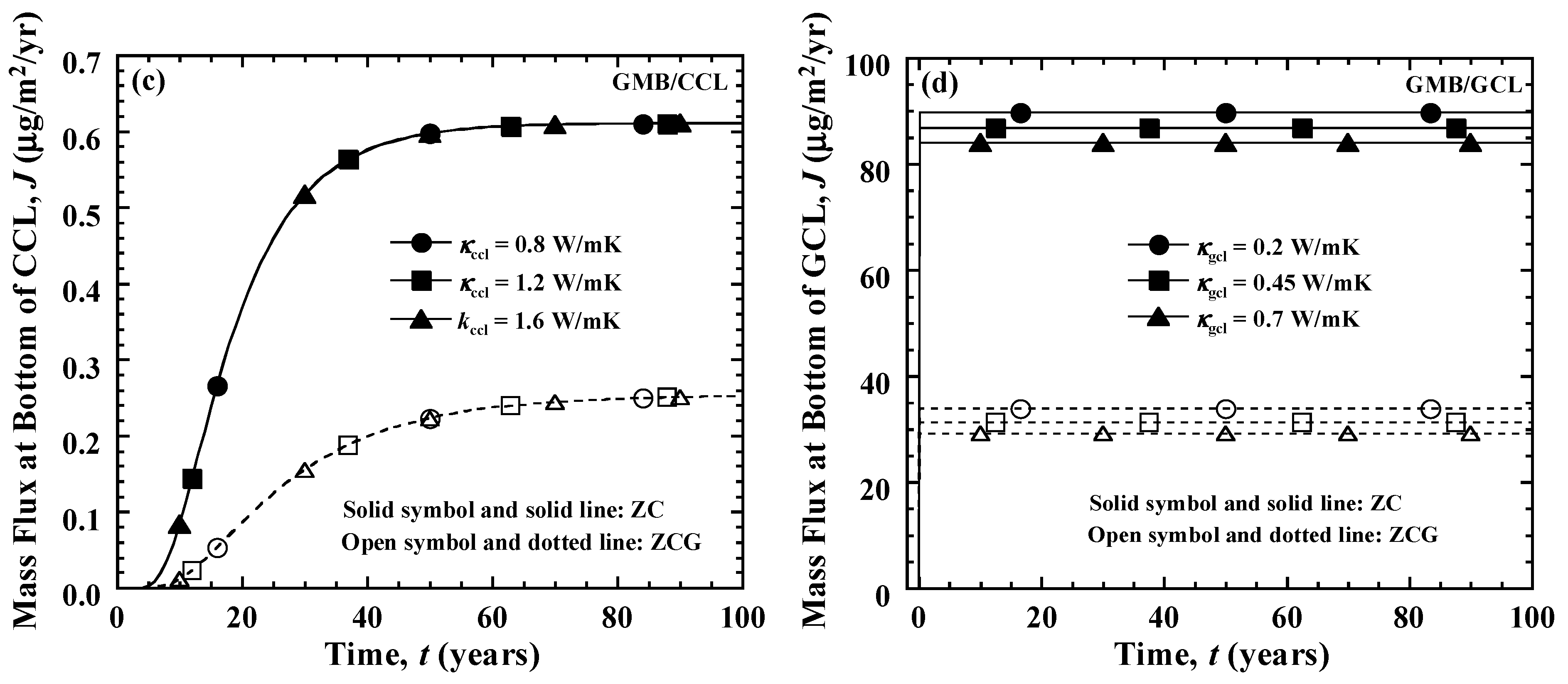
Hu et al. [58] reported the thermal conductivity of HDPE polymer ranging from 0.4 to 0.45 W/mK. According to the laboratory measurement data, the thermal conductivity of the GMB is around 0.3 W/mK [48,49]. Data for CCL thermal conductivity are scarce; this study adopts values for clay ranging from 0.9 to 3 W/mK [59,60,61]. For GCLs, laboratory measurements show thermal conductivities between 0.2 and 0.7 W/mK [36]. To illustrate the effect of thermal conductivity on benzene transport through the GMB/CL composite liner system, benzene mass flux J at the bottom of the liner system was calculated with ${\kappa }_{\mathrm{gmb}}$ (=0.3, 0.4 and 0.5 W/mK), ${\kappa }_{\mathrm{ccl}}$ (=0.8, 1.2 and 1.6 W/mK) and ${\kappa }_{\mathrm{gcl}}$ (=0.2, 0.45 and 0.7 W/mK), respectively. The chosen ${\kappa }_{\mathrm{gmb}}$ and ${\kappa }_{\mathrm{ccl}}$ are the same as those used by Peng et al. [26] for their investigation on contaminant transport through a GMB/CCL liner system.

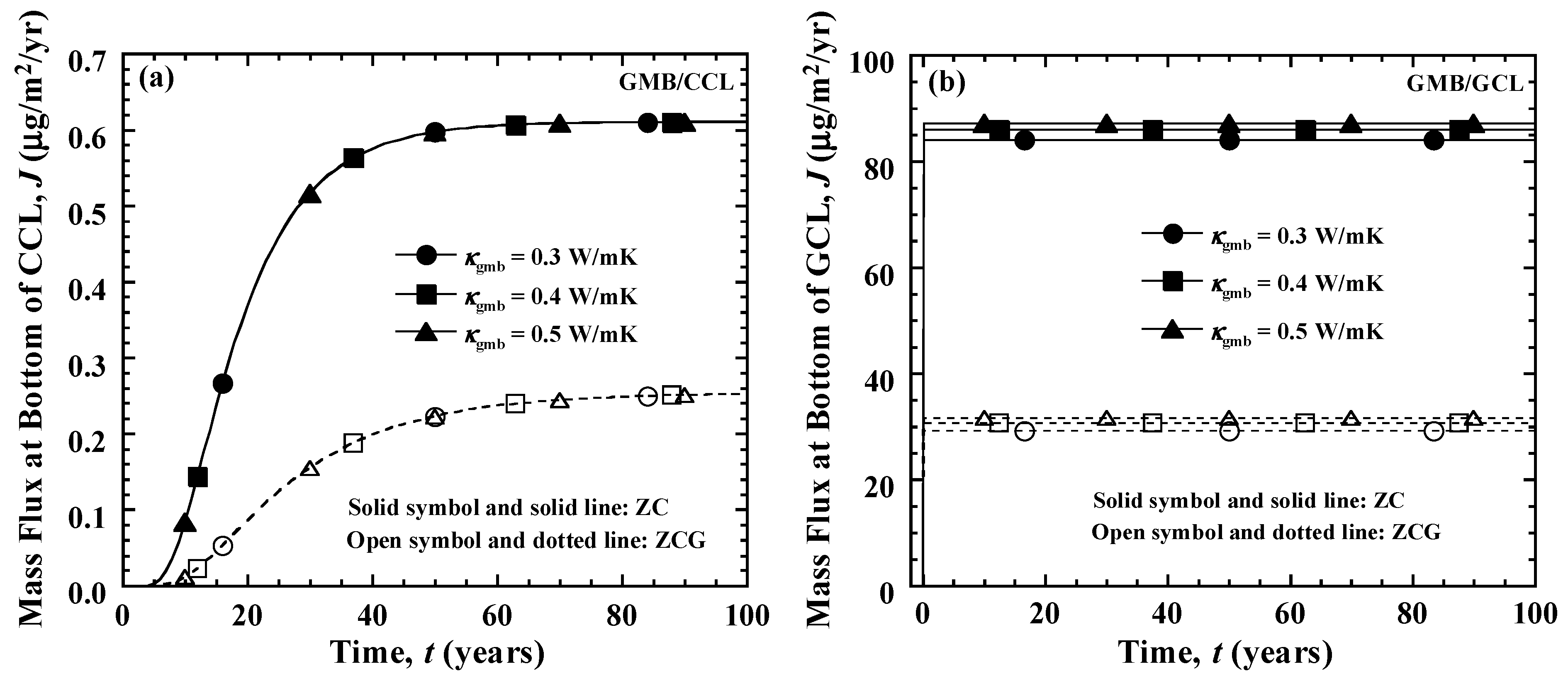
Figure 8a,c presents the J curves for the GMB/CCL composite liner system. For either ZC or ZCG boundary condition, all the ${\kappa }_{\mathrm{gmb}}$ and ${\kappa }_{\mathrm{ccl}}$ produce the same J curves throughout the 100 yr. simulation period, because GMB is very thin relative to CCL, and, thus, the ${\kappa }_{\mathrm{gmb}}$ and κ_ccl can hardly change the temperature distribution in the GMB/CCL composite liner system. In contrast, Figure 8b,d for the GMB/GCL system show that the thermal conductivities of the GMB and GCL have significant effects. Because the GMB thickness is not negligible relative to the GCL, higher ${\kappa }_{\mathrm{gmb}}$ increases the temperature gradient in the GCL, while higher ${\kappa }_{\mathrm{gcl}}$ reduces that gradient. Consequently, J increases with increasing ${\kappa }_{\mathrm{gmb}}$ and decreasing ${\kappa }_{\mathrm{gcl}}$.

6. Summary and Conclusions

This paper developed fully transient analytical solutions for organic contaminant transport through GMB/CCL and GMB/GCL composite liner systems, incorporating the coupled effects of advection through GMB defects, first-order degradation, and thermodiffusion. The proposed analytical solution was validated against experimental data, an existing analytical solution, and a finite-element numerical model. It is sufficiently accurate for GMB/CCL systems under all conditions. For GMB/GCL systems, it captures the general trends and provides conservative estimates for preliminary design, though the constant D_g and K_g assumption in the GMB introduces non-negligible errors. For a final detailed design requiring high accuracy, a full numerical simulation incorporating temperature-dependent properties is recommended. Using the validated solutions, a parametric study was performed to evaluate the impacts of thermodiffusion, Soret coefficient, and thermal conductivity on benzene transport. The main findings are summarized as follows:

(1) Thermodiffusion significantly accelerates benzene transport in both GMB/CCL and GMB/GCL. For the GMB/CCL system under a zero-concentration bottom boundary, increasing the temperature difference from 0 to 80 K increased the steady-state mass flux by 71%. Neglecting thermodiffusion can substantially underestimate contaminant outflow, leading to unsafe liner design.

(2) The effect of thermodiffusion is more pronounced in intact GMB liners than in damaged ones, because advection dominates when defects are present and weakens the relative contribution of thermodiffusion. The GMB/GCL system exhibits much higher benzene mass flux and stronger temperature response than the GMB/CCL system due to its smaller thickness.

(3) The benzene transport rate increases almost linearly with the Soret coefficient for both liner systems and both bottom boundary conditions. The zero-concentration-gradient condition shows a larger relative increase (up to 2102% when S_T increases from 0 to 0.005 K⁻¹ in the GMB/GCL system) because thermodiffusion becomes the primary driving mechanism.

(4) Thermal conductivity effects depend on the liner type. In the GMB/GCL system, higher GMB thermal conductivity and lower GCL thermal conductivity increase benzene transport by altering the temperature gradient within the GCL. In contrast, thermal conductivities of the GMB and CCL have negligible effects on the GMB/CCL system because the CCL dominates the total thickness.

(5) The proposed analytical solutions provide a computationally efficient tool for preliminary liner design, parametric sensitivity analysis, and early-stage risk assessment. They enable (i) rapid comparison of GMB/CCL and GMB/GCL systems to select environmentally preferable materials, (ii) optimization of clay liner thickness to balance containment performance against material consumption, and (iii) quantification of temperature effects to inform thermal mitigation strategies. The closed-form expressions offer explicit physical insights into the relationships between key transport parameters and liner performance, which are often obscured in numerical models. The analytical solution also serves as a reliable benchmarking tool for verifying numerical implementations.

References

1. Rowe, R.K. Geosynthetics and the minimization of contaminant migration through barrier systems beneath solid waste. In Proceedings of the Sixth International Conference on Geosynthetics, Atlanta, GA, USA, 25–29 March 1998; pp. 27–102. [Google Scholar]
2. Bonaparte, R.; Daniel, D.E.; Koerner, R.M. Assessment and Recommendations for Improving the Performance of Waste Containment Systems; EPA Report EPA/600/R-02/099; U.S. Environmental Protection Agency: Washington, DC, USA, 2002.
3. USEPA (United States Environmental Protection Agency). Resource Conservation and Recovery Act Orientation Manual; USEPA: Washington, DC, USA, 2014; Volume EPA530-F-11-003.
4. Kalbe, U.; Muller, W.; Berger, W.; Eckardt, J. Transport of organic contaminants within composite liner systems. Appl. Clay Sci. 2002, 21, 67–76. [Google Scholar] [CrossRef] [Scilit]
5. Park, J.K.; Sakti, J.P.; Hoopes, J.A. Transport of organic compounds in thermoplastic geomembranes. I: Mathematical model. J. Environ. Eng. 1996, 122, 800–806. [Google Scholar] [CrossRef] [Scilit]
6. Bouazza, A. Geosynthetic clay liners. Geotext. Geomembr. 2002, 20, 3–17. [Google Scholar] [CrossRef] [Scilit]
7. Rowe, R.K. Long-term performance of contaminant barrier systems. Geotechnique 2005, 55, 631–678. [Google Scholar] [CrossRef] [Scilit]
8. Xie, H.; Jiang, Y.; Zhang, C.; Feng, S. An analytical model for volatile organic compound transport through a composite liner consisting of a geomembrane, a GCL, and a soil liner. Environ. Sci. Pollut. Res. 2015, 22, 2824–2836. [Google Scholar]
9. Chen, Y.; Wang, Y.; Xie, H. Breakthrough-time based design of landfill composite liners. Geotext. Geomembr. 2015, 43, 196–206. [Google Scholar]
10. Feng, S.; Peng, M.; Chen, H.; Chen, Z. Fully transient analytical solution for degradable organic contaminant transport through GMB/GCL/AL composite liners. Geotext. Geomembr. 2019, 47, 282–294. [Google Scholar] [CrossRef] [Scilit]
11. Feng, S.; Peng, M.; Chen, Z.; Chen, H. Transient analytical solution for one-dimensional transport of organic contaminants through GM/GCL/SL composite liner. Sci. Total Environ. 2019, 650, 479–492. [Google Scholar] [CrossRef] [Scilit] [PubMed]
12. Davis, G.B.; Patterson, B.M.; Johnston, C.D. Aerobic bioremediation of 1,2 dichloroethane and vinyl chloride at field scale. J. Contam. Hydrol. 2009, 107, 91–100. [Google Scholar] [CrossRef] [Scilit] [PubMed]
13. Pu, H.; Qiu, J.; Zhang, R.; Zheng, J. Assessment of consolidation-induced VOC transport for a GML/GCL/CCL composite liner system. Geotext. Geomembr. 2018, 46, 455–469. [Google Scholar] [CrossRef] [Scilit]
14. Pu, H.; Qiu, J.; Zhang, R.; Zheng, J. Analytical solutions for organic contaminant diffusion in triple-layer composite liner system considering the effect of degradation. Acta Geotech. 2020, 15, 907–921. [Google Scholar]
15. Shackelford, C.D.; Lee, J. Analyzing diffusion by analogy with consolidation. J. Geotech. Geoenviron. Eng. 2005, 131, 1345–1359. [Google Scholar] [CrossRef] [Scilit]
16. Xie, H.; Zhang, C.; Feng, S.; Wang, Q.; Yan, H. Analytical model for degradable organic contaminant transport through a GMB/GCL/AL system. J. Environ. Eng. 2018, 144, 04018006. [Google Scholar] [CrossRef] [Scilit]
17. Qiu, J.; Pu, H.; Chen, X.; Zheng, J. Analytical solutions for contaminant diffusion in four-layer sediment-cap system for subaqueous in-situ capping. Geotext. Geomembr. 2021, 49, 376–387. [Google Scholar] [CrossRef] [Scilit]
18. Koerner, G.R.; Koerner, R.M. Long-term temperature monitoring of geomembranes at dry and wet landfills. Geotext. Geomembr. 2006, 24, 72–77. [Google Scholar] [CrossRef] [Scilit]
19. Rowe, R.K.; Hoor, A. Predicted temperatures and service lives of secondary geomembrane landfill liners. Geosynth. Int. 2009, 16, 71–82. [Google Scholar] [CrossRef] [Scilit]
20. Rowe, R.K.; Islam, M.Z. Impact of landfill liner time–temperature history on the service life of HDPE geomembranes. Waste Manag. 2009, 29, 2689–2699. [Google Scholar] [CrossRef] [Scilit] [PubMed]
21. Bouazza, A.; Singh, R.M.; Rowe, R.K.; Gassner, F. Heat and moisture migration in a geomembrane-GCL composite liner subjected to high temperatures and low vertical stresses. Geotext. Geomembr. 2014, 42, 555–563. [Google Scholar] [CrossRef] [Scilit]
22. Engelhardt, G.R.; Lvov, S.N.; Macdonald, D.D. Importance of thermal diffusion in high temperature electrochemical cells. J. Electroanal. Chem. 1997, 429, 193–201. [Google Scholar] [CrossRef] [Scilit]
23. Rosanne, R.; Paszkuta, M.; Tevissen, E.; Adler, P.M. Thermodiffusion in compact clays. J. Colloid Interface Sci. 2003, 267, 194–203. [Google Scholar] [CrossRef] [Scilit] [PubMed]
24. Xie, H.; Zhang, C.; Sedighi, M.; Thomas, H.R.; Chen, Y. An analytical model for diffusion of chemicals under thermal effects in semi-infinite porous media. Comput. Geotech. 2015, 69, 329–337. [Google Scholar] [CrossRef] [Scilit]
25. Yan, H.; Sedighi, M.; Xie, H. Thermally induced diffusion of chemicals under steady-state heat transfer in saturated porous media. Int. J. Heat Mass Transf. 2020, 153, 119664. [Google Scholar] [CrossRef] [Scilit]
26. Peng, M.; Feng, S.; Chen, H.; Chen, Z.; Xie, H. Analytical model for organic contaminant transport through GMB/CCL composite liner with finite thickness considering adsorption, diffusion and thermodiffusion. Waste Manag. 2020, 120, 448–458. [Google Scholar] [PubMed]
27. Qiu, J.; He, Y.; Song, D.; Tong, J. Analytical solution for solute transport in a triple liner under non-isothermal conditions. Geosynth. Int. 2022, 30, 364–381. [Google Scholar]
28. Qiu, J.; Jiang, L.; Pu, H.; Song, D.; Min, M.; Tong, J. Analytical solutions for contaminant transport through a GMB/CCL composite liner system considering effective porosity and thermodiffusion. Comput. Geotech. 2023, 163, 105713. [Google Scholar] [CrossRef] [Scilit]
29. Jiang, W.; Ge, S.; Feng, C.; Li, J. Transport of heavy metal contaminants in a composite liner under non-isothermal condition. Geosynth. Int. 2024, 31, 487–504. [Google Scholar] [CrossRef] [Scilit]
30. Qiu, J.; Pan, J.; Song, D.; Hu, B.; Tong, J.; Zhou, X. Assessment of heat transfer-induced contaminant transport for a GMB/GCL/CCL liner system. Int. J. Numer. Anal. Methods Geomech. 2025, 49, 4258–4275. [Google Scholar] [CrossRef] [Scilit]
31. Ruhl, J.L.; Daniel, D.E. Geosynthetic clay liners permeated with chemical solutions and leachates. J. Geotech. Geoenviron. Eng. 1997, 123, 369–381. [Google Scholar] [CrossRef] [Scilit]
32. Shackelford, C.D. Waste-soil interactions that alter hydraulic conductivity. In STP 1142 Hydraulic Conductivity and Waste Contaminant Transport in Soil; Daniel, D.E., Trautwein, S.J., Eds.; ASTM: West Conshohoken, PA, USA, 1994; pp. 111–168. [Google Scholar]
33. Park, J.K.; Nibras, M. Mass flux of organic chemicals through polyethylene geomembranes. Water Environ. Res. 1993, 65, 227–237. [Google Scholar] [CrossRef] [Scilit]
34. Rowe, R.K.; Mukunoki, T.; Lindsay, H. Effect of temperature on BTEX permeation through HDPE and fluorinated HDPE geomembranes. Soils Found. 2011, 51, 1103–1114. [Google Scholar] [CrossRef] [Scilit]
35. Mon, E.E.; Hamamoto, S.; Kawamoto, K.; Komatsu, T.; Moldrup, P. Temperature effects on solute diffusion and adsorption in differently compacted kaolin clay. Environ. Earth Sci. 2016, 75, 562. [Google Scholar] [CrossRef] [Scilit]
36. Bouazza, A.; Ali, M.A.; Rowe, R.K.; Gates, W.P.; El-Zein, A. Heat mitigation in geosynthetic composite liners exposed to elevated temperatures. Geotext. Geomembr. 2017, 45, 406–417. [Google Scholar] [CrossRef] [Scilit]
37. Foose, G.J.; Benson, C.H.; Edil, T.B. Analytical equations for predicting concentration and mass flux from composite liners. Geosynth. Int. 2001, 8, 551–575. [Google Scholar] [CrossRef] [Scilit]
38. Rowe, R.K.; Brachman, R.W. Assessment of equivalence of composite liners. Geosynth. Int. 2004, 11, 273–286. [Google Scholar] [CrossRef]
39. EI-Zein, A.; Rowe, R.K. Impact on groundwater of concurrent leakageand diffusion of dichloromethane through geomembranes in landfillliners. Geosynth. Int. 2008, 15, 55−71. [Google Scholar] [CrossRef] [Scilit]
40. Sangam, H.P.; Rowe, R.K. Effect of surface fluorination on diffusion through a high density polyethylene geomembrane. J. Geotech. Geoenviron. Eng. 2005, 131, 694–704. [Google Scholar] [CrossRef] [Scilit]
41. Farquhar, G.J. Leachate: Production and characterization. Can. J. Civ. Eng. 1989, 16, 317–325. [Google Scholar] [CrossRef] [Scilit]
42. Rowe, R.K. Leachate characterization for MSW landfills. In Proceedings Sardinia 95, Fifth International Symposium on Sanitary Landfill; CISA: Cagliari, Italy, 1995; Volume 2, pp. 327–344. [Google Scholar]
43. Rowe, R.K.; Mukunoki, T.; Sangam, H.P. BTEX diffusion and sorption for a geosynthetic clay liner at two temperatures. J. Geotech. Geoenviron. Eng. 2005, 131, 1211–1221. [Google Scholar] [CrossRef] [Scilit]
44. Barroso, M.; Touze-Foltz, N.; Maubeuge, V.K.; Pierson, P. Laboratory investigation of flow rate through composite liner consisting of a geomembrane, a GCL and a soil liner. Geotext. Geomembr. 2006, 24, 139–155. [Google Scholar] [CrossRef] [Scilit]
45. Benson, C.; Zhai, H.; Wang, X. Estimating the hydraulic conductivity of compacted clay liners. J. Geotech. Eng. 1994, 120, 366–387. [Google Scholar] [CrossRef] [Scilit]
46. Petrov, R.J.; Rowe, R.K. Geosynthetic clay liner (GCL)-chemical compatibility by hydraulic conductivity testing and factors impacting its performance. Can. Geotech. J. 1997, 34, 863–885. [Google Scholar] [CrossRef]
47. Petrov, R.J.; Rowe, R.K.; Quigley, R.M. Selected factors influencing GCL hydraulic conductivity. J. Geotech. Geoenviron. Eng. 1997, 123, 683–695. [Google Scholar] [CrossRef] [Scilit]
48. Singh, R.M.; Bouazza, A. Thermal conductivity of geosynthetics. Geotext. Geomembr. 2013, 39, 1–8. [Google Scholar] [CrossRef] [Scilit]
49. Ali, M.A.; Bouazza, A.; Singh, R.M.; Gates, W.P.; Rowe, R.K. Thermal conductivity of geosynthetic clay liners. Can. Geotech. J. 2016, 53, 1510–1521. [Google Scholar] [CrossRef] [Scilit]
50. Rowe, R.K.; Chappel, M.J.; Brachman, R.W.I.; Take, W.A. Field study of wrinkles in a geomembrane at a composite liner test site. Can. Geotech. J. 2012, 49, 1196–1211. [Google Scholar] [CrossRef] [Scilit]
51. Chappel, M.J.; Brachman, R.W.; Take, W.A.; Rowe, R.K. Large-scale quantification of wrinkles in a smooth black HDPE geomembrane. J. Geotech. Geoenviron. Eng. 2012, 138, 671–679. [Google Scholar] [CrossRef] [Scilit]
52. Giroud, J.P.; Bonaparte, R. Geosynthetics in liquid-containing structures. In Geotechnical and Geoenvironmental Engineering Handbook; Springer: Boston, MA, USA, 2001; pp. 789–824. [Google Scholar]
53. Wu, X.; Shi, J.; He, J. Analytical solutions for diffusion of organic contaminant through GCL triple-layer composite liner considering degradation in liner. Environ. Earth Sci. 2016, 75, 1371. [Google Scholar] [CrossRef] [Scilit]
54. Rowe, R.K. Short- and long-term leakage through composite liners. The 7th Arthur Casagrande Lecture. Can. Geotech. J. 2012, 49, 141–169. [Google Scholar] [CrossRef] [Scilit]
55. Azad, F.M.; Rowe, R.K.; Elzein, A.; Airey, D. Laboratory investigation of thermally induced desiccation of GCLs in double composite liner systems. Geotext. Geomembr. 2011, 29, 534–543. [Google Scholar] [CrossRef] [Scilit]
56. Harris, A.P.; Mcdermott, C.; Kolditz, O.; Haszeldine, R.S. Modelling groundwater flow changes due to thermal effects of radioactive waste disposal at a hypothetical repository site near Sellafield. UK. Environ. Earth Sci. 2015, 74, 1589–1602. [Google Scholar] [CrossRef] [Scilit]
57. Lasaga, A.C. Princeton Series in Geochemistry: Kinetic Theory in the Earth Sciences; Princeton University Press: Princeton, NJ, USA, 1998. [Google Scholar]
58. Hu, M.; Yu, D.; Wei, J. Thermal conductivity determination of small polymer samples by differential scanning calorimetry. Polym. Test. 2007, 26, 333–337. [Google Scholar] [CrossRef] [Scilit]
59. Tang, A.M.; Cui, Y.J.; Le, T.T. A study on the thermal conductivity of compacted bentonites. Appl. Clay Sci. 2008, 41, 181–189. [Google Scholar] [CrossRef] [Scilit]
60. Tarnawski, V.R.; Momose, T.; McCombie, M.L.; Leong, W.H. Canadian field soils III. Thermal-conductivity data and modeling. Int. J. Thermophys. 2015, 36, 119–156. [Google Scholar]
61. Xu, Y.; Sun, D.A.; Zeng, Z.; Lv, H. Effect of aging on thermal conductivity of compacted bentonites. Eng. Geol. 2019, 253, 55–63. [Google Scholar] [CrossRef] [Scilit]
Figure 1. Configuration of GMB/CL composite liner system. (Solid Horizontal Lines: Denote physical boundaries and material interfaces. Triangular Symbol (▽): Indicates the free leachate surface (upper hydraulic boundary). Double-Headed Vertical Arrows: Indicate dimensional measurements. Vertical/Curved Flux Arrows: Represent mass and heat transport pathways.).
Sustainability 18 07354 g001
Figure 2. Comparison of sodium chloride concentration profile within the compact clay between the proposed analytical solution and the experimental results reported by Rosanne et al. [23]: (a) experiment 1, and (b) experiment 2.
Sustainability 18 07354 g002
Figure 3. Comparison between the proposed analytical solution and analytical solution of Peng et al. [26]: (a) contaminant concentration at the base of liner for ZCG boundary condition, and (b) contaminant mass flux at the base of liner for ZC boundary condition.
Sustainability 18 07354 g003
Figure 4. Comparison of benzene mass flux at the base of the liner between the proposed analytical solution and the COMSOL Multiphysics 5.4: (a) compared with simplified numerical solution for GMB/CCL composite liner system, (b) compared with full numerical solution for GMB/CCL liner system, (c) compared with simplified numerical solution for GMB/GCL composite liner system, and (d) compared with full numerical solution for GMB/GCL composite liner system.
Sustainability 18 07354 g004
Figure 5. Benzene mass flux at the base of liner for different ∆T: (a) GMB/CCL composite liner system, and (b) GMB/GCL composite liner system.
Sustainability 18 07354 g005
Figure 6. Benzene mass flux at the base of liner for different liner systems: (a) CCL-based liner systems, and (b) GCL-based liner systems.
Sustainability 18 07354 g006
Figure 7. Benzene mass flux at the base of liner for different ST: (a) GMB/CCL liner system, and (b) GMB/GCL composite liner system.
Sustainability 18 07354 g007
Figure 8. Benzene mass flux at the base of liner for different thermal conductivities: (a) GMB/CCL composite liner system with varying GMB thermal conductivity, (b) GMB/GCL composite liner system with varying GMB thermal conductivity, (c) GMB/CCL composite liner system with varying CCL thermal conductivity, and (d) GMB/GCL composite liner system with varying GCL thermal conductivity.
Sustainability 18 07354 g008aSustainability 18 07354 g008b