Improving Scope 3.1 Carbon Accounting: A Framework for Selecting Weight-Based Material Emission Factors

Abstract

Scope 3.1 emissions from purchased goods and services often represent a substantial share of corporate greenhouse gas footprints, yet their quantification is characterized by high uncertainty and limited transparency. In practice, organizations frequently rely on weight-based secondary emission factors, which can vary substantially depending on underlying assumptions such as production technology or geographical origin. Existing standards and data quality approaches provide important guidance on representativeness, reliability, and data exchange, but offer limited operational support for selecting appropriate emission factors. This study addresses this practical challenge by examining emission-factor variability for selected material groups, identifying key influencing factors, and developing a qualitative decision-support framework for evaluating, selecting, and documenting secondary emission factors in Scope 3.1 accounting. The results demonstrate that emission factors for the same material can differ by more than an order of magnitude, leading to substantial deviations in carbon footprint results if selected inconsistently. The proposed framework, while not replacing supplier-specific primary data or formal data-quality assessment, reduces selection-related uncertainty, and supports more reliable carbon accounting, particularly in data-constrained supply chain contexts. By providing a transparent screening logic for early-stage Scope 3.1, the study enables more informed sustainability and procurement decisions.

1. Introduction

Climate change is widely established in the scientific literature and is primarily attributed to anthropogenic activities since the beginning of the industrial revolution [1,2]. Beyond temperature increases, it also amplifies both physical and transition risks for societies and value chains, making mitigation and adaptation central pillars of sustainability management. The Intergovernmental Panel on Climate Change (IPCC) Sixth Assessment Report, concludes that global warming is likely to exceed 1.5 °C this century [3]. Accordingly, pathways consistent with the 1.5 °C limit require greenhouse gas emissions to decline by 84%, alongside global CO₂ emissions reaching net zero around 2050 [3,4,5,6].

In general, the stocks and flows of materials, energy and other resources in production have a major environmental impact, underscoring the need for systematic assessment, management, and mitigation of emissions associated with material flows [7,8]. For example, global resource extraction and processing account for over 60% of planet-warming emissions, whereas iron and steel production is responsible for about 7% of energy-sector CO₂ emissions, while cement production alone accounts for around 7% of global CO₂ emissions [9,10,11]. This requires quantifying process- and product-related emissions and disclosing them as a carbon footprint. While established carbon accounting standards like such as the GHG Protocol and ISO 14040/14044, provide a robust basis, the credibility and decision-usefulness of results ultimately depend on their consistent and correct application in practice [12].

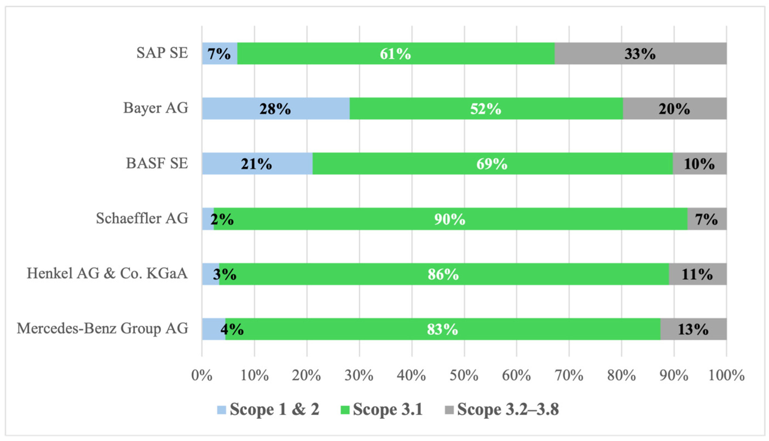
A generally recognized standard for corporate GHG accounting is the overarching corporate standard of the GHG Protocol [13] and its supplements: the Product Standard [14] and the Scope 3 Standard [15]. For many manufacturing companies, the largest share of GHG emissions are not generated by direct in-house production or processing by the company itself (Scopes 1 and 2: energy combustion and purchased energy), but in the upstream and downstream processes (Scope 3: company’s value chain, e.g., material suppliers, external logistics providers, etc.) [4,16,17,18,19]. As shown in Figure 1, Scope 3.1 (purchased goods and services) emissions specifically account on average for more than 70% across manufacturing industries. For the manufacturing companies listed, the share of Scope 3.1 is between 60 and 90% of upstream and in-house CO₂e emissions. Only for the energy-intensive companies BASF SE and Bayer AG does Scope 3.1 account for only between 50 and 70%. These figures are not intended as a representative cross-industry sample, nor does it provide direct empirical evidence for small- and medium-sized enterprises. However, the relevance of Scope 3.1 is not determined by company size alone, but also by the material intensity, production depth, sourcing structure, and energy profile of the business model. Material-oriented SMEs operating in similar value chains may therefore face comparable upstream emission patterns, particularly when purchased materials and components dominate their product carbon footprint while direct operational emissions remain comparatively limited. At the same time, SMEs often have fewer resources and less bargaining power to obtain supplier-specific primary data. This makes transparent and defensible use of secondary emission factors particularly relevant for early-stage Scope 3.1 accounting in SME contexts.

While it is still comparatively tractable for large companies (persons employed ≥ 250, annual turnover ≥ €50 million or a balance sheet total ≥ €25 million) to determine their direct Scope 1 and Scope 2 emissions, indirect Scope 3 emissions pose a substantially greater methodological and operational challenge due to the complexity and opacity of multi-tier value chains. This challenge is not confined to a single company size class: Large enterprises often face substantial data gaps across suppliers and logistics partners due to limited transparency, fragmented multi-tier value chains, and methodological inconsistencies in Scope 3 reporting. In addition, the high implementation effort, coordination requirements, and cost implications associated with sustainability initiatives further complicate effective data integration across existing organizational systems [26,27,28,29,30]. Smaller suppliers, including many small- and medium-sized enterprises (SME), are often affected indirectly, as reporting requirements and data requests are cascaded through supply chains by larger customers and regulators. In practice, limited resources and restricted access to supplier-specific primary data can further constrain the quality and granularity of Scope 3.1 accounting for these actors [12,31,32,33,34].

From a life cycle assessment (LCA) perspective, these challenges closely parallel well-documented limitations of LCA studies, particularly with regard to the high parametric uncertainty associated with generic secondary data sources, limited transparency of underlying assumptions, and insufficient resolution in hotspot identification. Such deficits can lead to distorted results and significantly reduce the informative value of both LCA studies and corporate carbon footprints [35,36,37,38,39]. This issue is especially pronounced in the assessment of purchased goods (Scope 3.1), which account for a dominant share of total GHG emissions for many organizations (see Figure 1) but are often characterized by sparse and heterogeneous data availability.

Against this background, this paper develops a systematic, low-barrier methodology that supports organizations across company sizes in estimating indirect Scope 3.1 emissions, with particular relevance for resource-constrained actors and supply-chain settings where supplier-specific primary data are unavailable. Since many organizations, especially those with limited bargaining power in supplier relationships, which are often SMEs, cannot obtain CO₂e primary data (PD) directly from their suppliers in the early reporting cycles, they frequently rely on secondary data (SD). SD includes industry-average data (e.g., from published databases, government statistics, and industry associations), financial data, and other generic data [15].

Despite their widespread use, the selection of appropriate secondary emission factors (EFs) (e.g., kgCO₂e/kg of steel) remains a major challenge in practice. Searches in life cycle inventory databases often yield a substantial variance in EF values for the same material, without clear guidance on which value best represents the actual conditions of a specific case. Consequently, practitioners frequently apply overly aggregated material categories or select emission factors without systematically evaluating their underlying assumptions, leading to potentially large distortions in carbon accounting results.

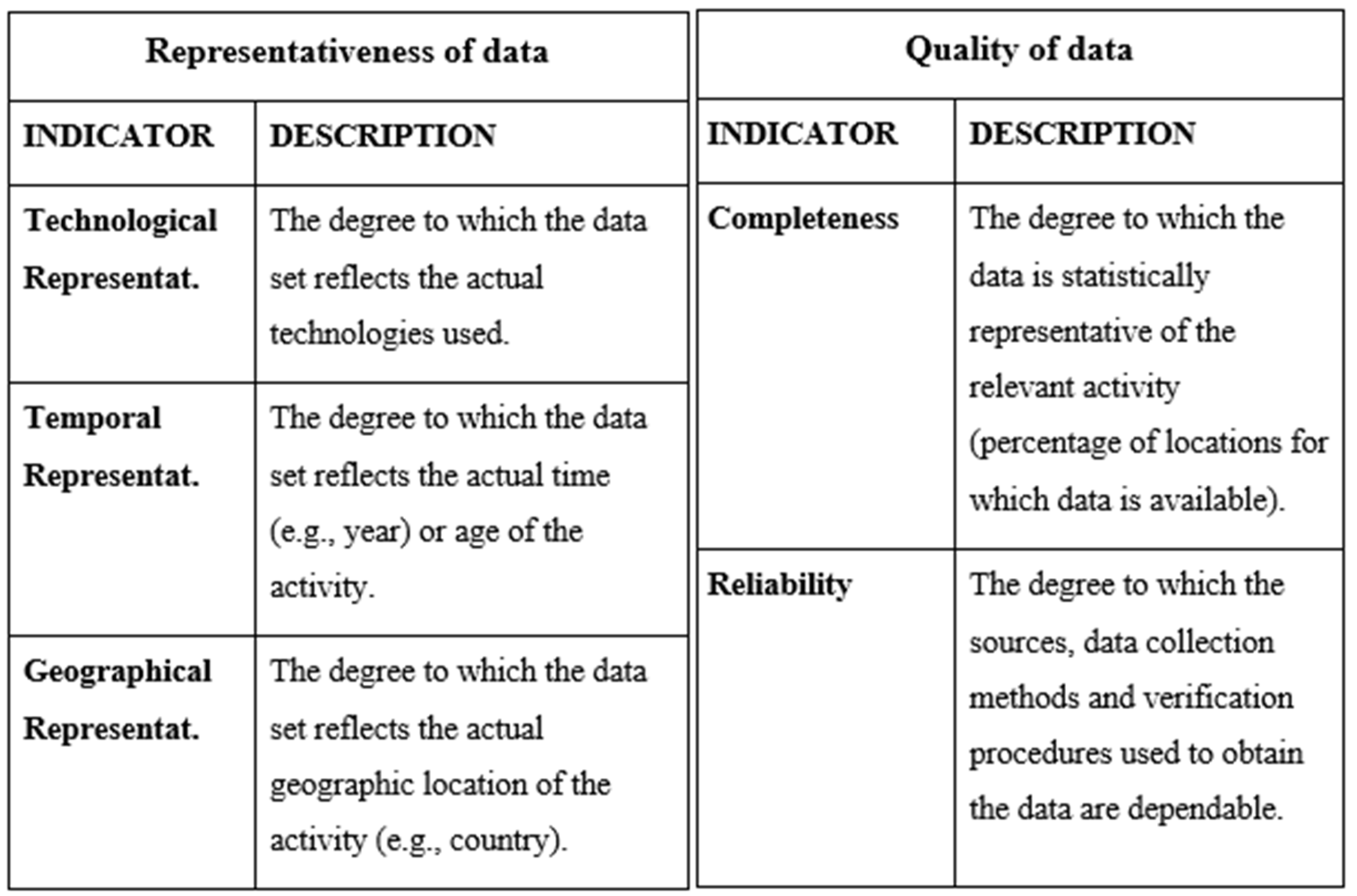
Several established standards and frameworks already address data quality and transparency in greenhouse gas accounting and life cycle assessment. The GHG Protocol Scope 3 Standard defines general data quality indicators such as technological, temporal, and geographical representativeness, completeness, and reliability [40]. LCA-based approaches such as the Product Environmental Footprint method [41] and ecoinvent data quality guidelines with pedigree-matrix-based uncertainty assessment [42] provide further guidance for evaluating datasets and documenting representativeness. Recent initiatives such as PACT additionally support the standardization and exchange of product carbon footprint information across value chains [43]. ISO 14071 strengthens the credibility of LCA studies by specifying requirements for critical review processes and reviewer competencies [44].

However, these approaches primarily address data quality assessment, product carbon footprint exchange, or review procedures at a broader methodological level. They provide limited practical guidance for a common operational problem in early-stage Scope 3.1 accounting. When a practitioner searches for a material in a database and receives several weight-based secondary emission factors, it is often unclear which dataset best represents the actual material purchased by the reporting company. The challenge is therefore not only whether a dataset is generally of high quality, but whether its underlying assumptions align with the case-specific material conditions, such as production route, energy mix, recycled content, processing stage, and geographical context.

This study addresses this gap by developing a qualitative evaluation and selection framework for weight-based secondary emission factors, explicitly tailored to purchased goods under Scope 3.1. The framework does not aim to replace supplier-specific primary data, existing data quality indicators, or formal LCA review procedures. Instead, it complements them by translating material-specific influencing factors into a structured, transparent, and practically applicable decision logic for situations in which primary data are unavailable and practitioners must rely on secondary emission factors.

By doing so, this paper contributes to the existing literature in three ways: (1) it provides a structured analysis of the magnitude and drivers of variability in material-related emission factors for selected material groups, (2) it identifies and structures the key determinants underlying this variability, and (3) it introduces a qualitative decision-support framework that can assist practitioners in evaluating, selecting, and documenting secondary emission factors more transparently under constrained data availability.

2. State of the Art

The following sections outline the methodological foundations of greenhouse gas accounting and the data quality considerations associated with different emission calculation methods. Section 2.1 introduces the relevant standards, accounting boundaries, emission scopes, and calculation logic underlying corporate value-chain and product-level GHG accounting. Building on this basis, Section 2.2 describes how the use of supplier-specific, average-data, spend-based, and hybrid methods affects the quality, specificity, and reliability of Scope 3.1 emission estimates.

2.1. Fundamentals of GHG Accounting

Corporate greenhouse gas accounting at the value-chain level is governed by a constellation of complementary standards. At the product level, ISO 14040 [45] and ISO 14044 [46] establish the methodological foundations of life cycle assessment (LCA), while ISO 14067 [47] operationalizes these principles for product carbon footprint quantification. At the organizational level, ISO 14064-1 [48] and the GHG Protocol Corporate Value Chain (Scope 3) Standard [15] provide the predominant frameworks for structuring corporate GHG inventories. The Scope 3 Standard translates the life cycle logic of LCA into a corporate accounting architecture by categorizing indirect value-chain emissions across 15 standardized activity categories, commonly grouped into upstream (Categories 1–8) and downstream (Categories 9–15) emissions. Category 1—purchased goods and services (Scope 3.1), which is specifically relevant for this paper, includes all upstream emissions from the extraction, manufacture and transportation of products purchased or acquired by the reporting company in the reporting year [15]. This paper focuses on the calculation of carbon footprints of tangible products rather than services (intangible).

Scope 3.1 emissions are calculated by multiplying activity data (e.g., mass of material in kg) by a corresponding emission factor (EF; e.g., kgCO₂e/kg), as specified in the Scope 3 Standard and corroborated by established accounting practice [15,40]. The focus of this paper is on systematically characterizing the variability of these EFs depending on various influences. Companies can use two types of EFs to calculate Scope 3 emissions: Primary data (PD) directly by suppliers or secondary data (SD) from published databases, government statistics, literature studies and industry associations [15]. Based on these two types of data, different methods can in turn be used to calculate emissions from purchased goods (Scope 3.1 emissions): [40].

• Supplier-specific method: Collection of cradle-to-gate PD from suppliers on product-specific GHG emissions from the production of goods.
• Average-data method (Weight-based): Estimates emissions for goods by collecting activity data on the mass (e.g., kg) of goods purchased and multiplying it by the corresponding secondary cradle-to-gate EF (e.g., industry average; kg CO₂e/kg). Weight-based EFs are mainly found in process-based LCI (life cycle inventory) databases, such as GaBi, GEMIS, and ecoinvent, or via industry associations [49]. Weight-based EFs result from detailed bottom-up analyses of each individual step in the production process, where the corresponding input and output flows are precisely recorded [45]. A weight-based EF is more suitable for products where emissions are directly proportional to weight, such as raw materials.
• Spend-based method: Estimates the emissions for goods by collecting data on the economic value of the goods purchased (e.g., €) and multiplying it by the corresponding secondary (e.g., industry-standard) EF (e.g., kg CO₂e/€). Spend-based EFs originate from large-scale top-down economic models, so-called “Environmentally Extended Input–Output models” (EEIO) [50]. Popular sources for spend-based EFs are the British BEIS (Department for Business, Energy, and Industrial Strategy), the American EPA (Environmental Protection Agency), EXIOBASE (Extended Input–Output Database) and the OECD (Organization for Economic Co-operation and Development) Inter-Country Input–Output (ICIO) tables [40,51]. A spend-based EF is more appropriate for products where the price is more strongly correlated with emissions, such as services (e.g., consulting, administration) or very complex assemblies consisting of a variety of materials.
• Hybrid method: Combining the supplier-specific method (where data is available) with the average-data or spend-based method to close data gaps.

2.2. Data Quality of the Various Calculation Methods

Sources of primary and secondary data can be of different quality, which in turn is directly reflected in the meaningfulness of the various accounting methods:

• Supplier-specific method: Although the supplier-specific method based on PD is more specific to the individual supplier than methods based on SD [52,53], they do not necessarily lead to more accurate results. In fact, the PD obtained from a supplier may even be less accurate than the industry average (difference between data specificity and data accuracy). Accuracy derives from the granularity of the emission data, the reliability of the supplier’s data sources, and which allocation techniques were used [40]. At the same time, the supplier-specific method has to contend with the following difficulties: shortcomings in terms of data quality due to the lack of expertise of suppliers [51,54] and rare data availability due to the unwillingness of suppliers to share sensitive data [55,56], the high effort for suppliers, and insufficient market power of the reporting company [51].
• Average-data or spend-based method: SD based on average-data or spend are often readily available and can be used to enable rapid, resource-efficient approximations of the environmental impact of different materials.

  ○

  In addition to these advantages, spend-based values have the disadvantage that they are somewhat imprecise in terms of their actual environmental impact, as they are only based on financial data. Inflation, international exchange rate fluctuations or volume discounts granted would have an incomprehensible effect on reducing emissions. Therefore, spend-based EFs must be converted for the year of application using the currency inflation rate and an adjustment for VAT [51,57,58,59,60].

  ○

  Weight-based average-data have the disadvantage that their boundary conditions, i.e., the system boundaries drawn when considering them, are variable. Therefore, the EF for one and the same product can be inconsistent. For small total material volumes (e.g., a few kg of material) this is negligible, but multiplying the EF by thousands of tons of material will lead to a potentially material estimation error of the carbon footprint [12,57,58,60,61]. Another disadvantage is the poorer accessibility compared to spend-based EFs. Current, verified data values are often only available in paid databases.

As most SMEs have neither the necessary human resources nor the necessary market power to obtain PD from their suppliers, it is advisable for such organizations to rely on SD during initial reporting cycles. Spend-based SD are slightly easier to use, as they require less expertise in the area of material production. Weight-based SD—if the EFs are selected correctly—have the advantage of being somewhat more accurate, as they are based on detailed bottom-up analyses and are not subject to macroeconomic factors. The aim of this paper is therefore to mitigate the shortcomings of weight-based average-data and increase its attractiveness. To do so, companies must be provided with a profound information basis and methodology for classifying and selecting appropriate weight-based Scope 3.1 CO₂e SD. However, the so far available data quality indicators mentioned in the Scope 3 Standard (see Figure 2) are only rough guidelines for checking the quality of data. Beyond these indicators, neither the GHG Protocol Standards nor any other widely adopted framework provides operational criteria for evaluating, comparing, or classifying weight-based or spend-based SD at the material level. This constitutes the central methodological gap addressed by the present study.

3. Methods

This study follows a structured multi-step research design combining literature analysis, data collection from LCI databases, and qualitative framework development. The methodological approach aims to analyze the variability of weight-based emission factors, identify the key factors influencing their magnitude, and develop and apply a framework for their evaluation and selection in Scope 3.1 accounting.

3.1. Literature Review

A targeted literature review was conducted to establish the conceptual foundation of the study and to identify existing approaches to Scope 3 accounting, emission factor selection, and data quality assessment.

The review included peer-reviewed journal articles, review papers, and conference publications retrieved from the databases ScienceDirect, MDPI Open Access Journals, SpringerLink, and Google Scholar. Search terms included combinations of “Scope 3 emissions”, “Scope 3.1 purchased goods”, “emission factors”, “secondary data”, “life cycle assessment data quality”, “product environmental footprint” and “product carbon footprint data exchange”.

The search was conducted between October 2025 and January 2026. To ensure topical relevance, priority was given to publications from 2021 onwards, while foundational standards (e.g., GHG Protocol, ISO standards, PACT and PEF-related documents) were included irrespective of publication year. Based on this screening the selected relevant publications were used to substantiate the specific operational challenge addressed by this study: the absence of a low-barrier, material-specific decision logic for selecting among multiple weight-based secondary emission factors in Scope 3.1 accounting.

3.2. System Boundaries and Accounting Approach

The study adopts a cradle-to-gate perspective consistent with established LCA standards (ISO 14040/44, ISO 14067) and the GHG Protocol Product and Scope 3 Standards. Emissions are calculated using the weight-based average-data method, where activity data (mass of purchased materials) are multiplied by corresponding emission factors (kgCO₂e/kg material).

The focus is on weight-based secondary data, as this approach is widely used in practice when supplier-specific primary data are unavailable—particularly in early stages of Scope 3 reporting and in resource-constrained contexts such as SMEs [40,62]. Compared to spend-based approaches, weight-based emission factors provide higher process resolution but require heightened sensitivity to system boundary specification due to their sensitivity to system boundaries and production conditions.

3.3. Data Collection

To analyze the variability of emission factors, a systematic data collection was conducted for five representative material groups (steel, aluminum, copper, polypropylene, and polyamide), covering 23 specific material variants. The material selection was case-driven and based on the most relevant material groups identified in the context of a research project in which carbon accounting was conducted. Metals and polymers were therefore selected because they represented the dominant material groups in the available bill-of-materials and supplier-related documentation.

Two types of data sources were used:

(1)

Publicly accessible databases and literature sources:

For the analysis of emission factor variability (Section 4.1), emission factors were collected from publicly available databases, registers, and literature sources (e.g., governmental databases such as ProBas, industry publications). This choice reflects real-world conditions, where many organizations—particularly SMEs—initially rely on accessible but heterogeneous data sources.

(2)

Process-based LCI database (ecoinvent):

For the identification of influencing factors (Section 4.2), datasets from the ecoinvent database (version 3.11, system model: cutoff) were analyzed. Relevant datasets were selected from the ISIC categories “Mining and quarrying” and “Manufacturing”, covering complete production chains from raw material extraction to final processing.

In cases where no single dataset represented the full cradle-to-gate chain, production chains were reconstructed by linking multiple datasets to represent full cradle-to-gate processes. Supplementary literature (more than 25 sources) was used to contextualize production routes and validate interpretations of dataset characteristics.

3.4. Data Analysis

The collected emission factors were analyzed in two steps:

(1)

Variability analysis:

Emission factors were grouped by material category and further differentiated according to key characteristics such as production route, geographical origin, and processing level. For each material variant, multiple emission factors (typically 2–4 values) were compared to assess variability. The range of variation was expressed using minimum–maximum ratios (MIN–MAX factors), indicating the relative spread between the highest and lowest values.

(2)

Identification of influencing factors:

To explain observed variability, the ‘Dataset Description’ sections of the ecoinvent datasets were systematically screened. Relevant parameters describing system boundaries and production conditions were extracted and categorized.

This analysis resulted in the identification of five key influencing factors. These factors were grouped into higher-level categories to structure their interdependencies.

3.5. Framework Development

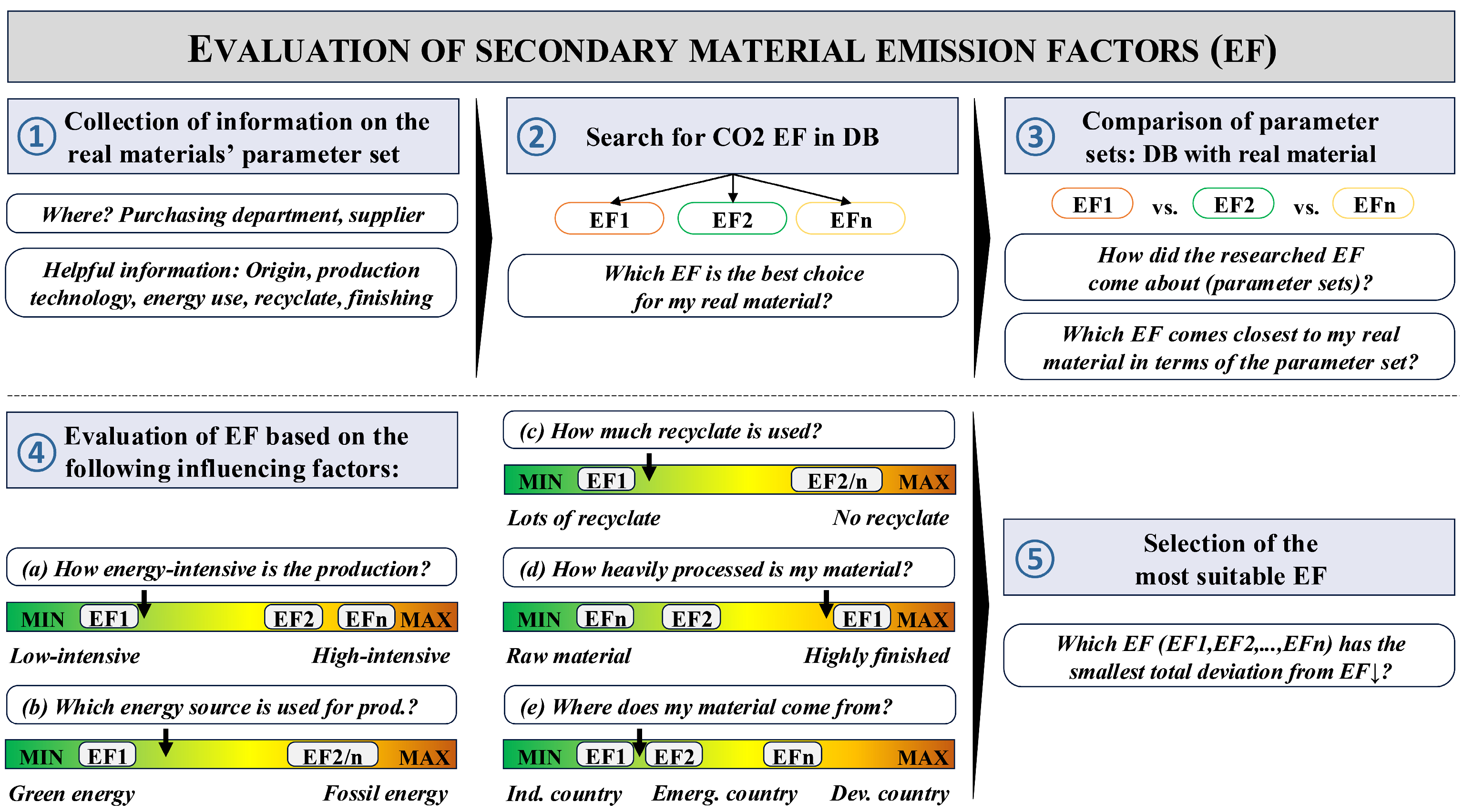
Based on the identified influencing factors, a qualitative evaluation and selection framework was developed. The framework translates the five influencing factors into qualitative scales, which are explained further in Section 4.2 and are visually shown in Figure 3, enabling the comparison between:

• The parameter set of a real material (case-specific conditions);
• The parameter sets underlying available emission factors from databases.

Each emission factor is assessed along the five dimensions, and the most suitable factor is selected based on its degree of parametric alignment to the real material conditions. The framework is intentionally designed as a qualitative decision-support tool to ensure applicability across different materials and data availability levels, avoiding overly specific quantitative weighting schemes. This design choice is justified by the methodological uncertainty and heterogeneity inherent in secondary emission factor selection, where differences in system boundaries, production contexts, data quality, and conversion factors can substantially affect the resulting carbon footprint. For this reason, the framework does not assign fixed numerical weights to the five influencing factors. Their relative importance may vary depending on the material and production route. For example, recycled content may dominate the emission profile of secondary metals, whereas production technology and process energy may be more decisive for primary material routes. Rather than suggesting a universally valid weighting scheme, the qualitative structure supports transparent, systematic, and practice-oriented decision-making while avoiding a false sense of precision. This is particularly relevant in Scope 3 accounting, where companies often rely on secondary or average data when supplier-specific primary data are unavailable, and where an initial screening based on less specific data is recommended before more precise data collection is prioritized [15,56]. Where a structured comparison is required, an unweighted comparison of the five influencing factors may be used as a transparent default heuristic. However, this default does not imply that the factors are statistically independent or equally causal across all materials. Practitioners should document the rationale for the selected emission factor and may deviate from the default comparison where material-specific knowledge indicates that one factor is clearly dominant. The framework should therefore be understood as a decision-support procedure that improves transparency and consistency, rather than as a deterministic optimization model.

3.6. Illustrative Application of the Framework

To demonstrate the practical applicability of the proposed framework and to explore its implications for emission results, the framework is applied to an illustrative material case and complemented by a structured sensitivity analysis. The illustrative application shows how the framework can be used to systematically compare emission factors based on material-specific parameters, such as production technology, energy mix, recyclate content, and degree of processing. This reflects typical real-world conditions in which multiple emission factors are available, but their suitability is non-transparent with respect to their contextual representativeness.

In addition, a sensitivity analysis is conducted to assess how strongly the resulting carbon footprint depends on the selection of emission factors. For this purpose, emission outcomes are compared across different plausible emission factor choices while keeping activity data constant. This facilitates isolating the effect of emission factor selection as a key source of uncertainty in Scope 3.1 accounting. The objective of this combined approach is not to provide a comprehensive empirical validation of the proposed framework. Rather, the paper serves as a proof of concept by demonstrating how the framework can be applied in practice and by illustrating the potential magnitude of its influence on carbon accounting results. The illustrative application shows how emission factors can be evaluated and selected across the proposed dimensions, while the sensitivity analysis highlights how alternative EF choices may lead to substantially different GHG balances. Thus, the paper provides an initial demonstration of the framework’s practical relevance and decision-support potential, while broader empirical validation remains a task for future research. The detailed results of both the illustrative application and the sensitivity analysis are presented and discussed in Section 4.

4. Results

The following chapter presents the key results of the study. It first examines the variance in CO₂e emission factors across materials and identifies the main factors influencing this variability. Building on these findings, a method for evaluating and selecting suitable Scope 3.1 CO₂e emission factors is developed. The chapter concludes with an illustrative application and sensitivity analysis to demonstrate the practical relevance of the proposed approach.

4.1. Variance in CO₂e Emission Factors of Materials

When sustainability managers of companies subject to reporting requirements are faced with the task of accounting for the Scope 3.1 CO₂e emissions of their purchased materials and have opted for a weight-based SD approach, they are faced with two main tasks: finding activity data (e.g., 500 kg of steel) and finding EFs (e.g., kgCO₂e/kg of steel). The latter constitutes the methodologically more demanding challenge of finding the correct EF for the respective materials.

A search for a specific material (e.g., “steel”) in an LCI database (paid or open access) leads to a whole collection of material-specific EFs. If no expert is involved, it is not obvious at first glance which EF applies to the real conditions of the material to be balanced and what needs to be considered when selecting the most suitable EF. Depending on the specific characteristics of the material, the EFs vary considerably (see

Table 1. CO₂e emission factors (EFs) for selected steel products in the unit [kg CO₂e per kg material] ¹.

Pos.	Steel Product	EF1	EF2	EF3	EF4	Mean	MIN–MAX
I-A	Primary blast furnace steel (RoW)	2.2	2.56	2.4	2.18	2.34	1.17
I-B	Primary blast furnace steel (EU)	1.9	1.71	1.76	1.7	1.77	1.12
I-C	Primary DRI steel (green H2) (EU)	0.34	0.09	0.05	-	0.16	6.80
I-D	Arc furnace steel (secondary) (EU)	0.2	0.45	0.55	0.3	0.38	2.75
I-E	Stainless steel (GLO)	3.39	6.29	5.2	5.18	5.02	1.86
I-F	Electrolyt. galvanized sheet (GLO)	2.6	2.42	-	-	2.51	1.17
I-G	Hot-dip galvanized sheet (GLO)	2.2	2.5	2.58	-	2.43	1.17
I-H	Tinplate (GLO)	3.1	2.57	2.62	-	2.76	1.21
I-I	Electrical sheet/Electric strip (GLO)	3.7	2.6	2.49	-	2.93	1.49

¹ Shown are four values (where available) taken from different databases, registers or other publicly available sources, their arithmetic mean and the MIN–MAX factor between the highest and lowest value (highest divided by lowest value) for each material. High MIN–MAX factors indicate a large variation range. The numbering of the material is used for easier referencing in the text. The magnitude of the CO₂e EFs shown in the table can be better understood by applying a color scale to all the values: The color gradient (red–yellow–green with gradations) was applied to the complete range of filled cells (across rows and columns). Red means a high EF, yellow a medium EF, green a low EF. The stronger the color, the more pronounced the attribute. Geographical abbreviations: EU (Europe), RoW (rest of world), GLO (global).

). The variation between the individual material-specific EF is based on various influencing factors (IFs) (e.g., material origin, production technology, energy use, degree of finishing, etc.), which are specified in more detail in Section 4.2. Table 1 provides an exemplary overview of a range of EFs [kgCO₂e/kg material] for selected steel products. The materials are labeled with an alphanumeric abbreviation (e.g., I-A-3: Table 1-line A-value 3). The values of the EFs are taken from various databases, registers or other publicly accessible sources (see Supplementary Materials Supporting Information S1 and S2).

Table 1 clearly shows that the EFs across the individual steel products (viewed vertically) are subject to an extremely large variation: from 0.05 to 6.29 kgCO₂e/kg {I-C-3, I-E-2}, meaning a MIN–MAX factor of approx. 125 between the highest and lowest value. This finding underscores a fundamental principle that extends beyond steel to all material categories: aggregating heterogeneous material variants under a single superordinate category such as “steel” and applying a uniform EF is methodologically inadmissible for accurate Scope 3.1 accounting. Such aggregation would apply a single emission intensity value to materials with fundamentally heterogeneous emission profiles, introducing systematic and potentially material distortions into the overall carbon footprint.

On the other hand, it is also clear from Table 1 that even within a specific steel product (viewed horizontally) there are sometimes large ranges of variation. These range from approx. 7% deviation (MIN–MAX factor 1.07) for electrolytically galvanized sheet {I-F} to 580% deviation (MIN–MAX factor 6.8) in the case of green steel produced with green hydrogen {I-C}. In addition to the IFs explained in Section 4.2, the reasons for the variation can also be attributed to the timeliness (time of data collection) and methodological inconsistencies in the datasets. The selection of a correct EF is therefore of crucial importance for the accuracy of the overall balance. For this purpose, the ‘Dataset Description’ section needs to be systematically evaluated for relevant system boundaries and the other IFs presented in Section 4.2.

The same correlations can be seen not only for steel, but also for other common materials, which are shown in

Table 2. CO₂e emission factors (EFs) for selected materials in the unit [kg CO₂e per kg material] ¹.

Pos.	Material	EF1	EF2	EF3	EF4	Mean	MIN–MAX
II-A	Primary polypropylene (GLO)	2.3	1.7	1.9	2.88	2.20	1.69
II-B	Polypropylene (secondary) (GLO)	0.97	-	-	-	0.97	1.00
II-C	Polypropylene (30% glass fiber reinforced) (GLO)	1.7	2.92	-	-	2.31	1.72
II-D	Polypropylene (40% glass fiber reinforced) (GLO)	0.98	2.9	-	-	1.94	2.96
II-E	Polyamide 6 (perlon) (GLO)	3.66	9.13	-	-	6.40	2.49
II-F	Polyamide 6 (30% glass fiber reinforced) (GLO)	7.22	-	-	-	7.22	1.00
II-G	Polyamide 6.6 (nylon) (GLO)	8.06	7.92	-	-	7.99	1.02
II-H	Polyamide 6.6 (30% glass fiber reinforced) (GLO)	6.45	6.97	-	-	6.71	1.08
II-I	Primary copper (EU)	3.3	4.87	-	-	4.09	1.48
II-J	Primary copper (RoW)	5.4	4.24	6.66	2.87	4.79	2.32
II-K	Copper (secondary) (EU)	1.73	1.7	1.78	1.98	1.80	1.16
II-L	Primary aluminum (RoW)	16.5	10.0	16.5	20.1	15.78	2.01
II-M	Primary aluminum (EU)	6.5	11.9	7.69	13.5	9.90	2.08
II-N	Aluminum (secondary) (EU)	0.52	1.04	-	-	0.78	2.00

¹ Shown are four values (where available) taken from different databases, registers or other publicly available sources, their arithmetic mean and the MIN–MAX factor between the highest and lowest value (highest divided by lowest value) for each materialHigh MIN–MAX factors indicate a large variation range. The numbering of the material is used for easier referencing in the text. The magnitude of the CO₂e EFs shown in the table can be better understood by applying a color scale to all the values: The color gradient (red–yellow–green with gradations) was applied to the complete range of filled cells (across rows and columns). Red means a high EF, yellow a medium EF, green a low EF. The stronger the color, the more pronounced the attribute. Geographical abbreviations: EU (Europe), RoW (rest of world), GLO (global).

. Here too, depending on certain IFs (Section 4.2), there are large variation ranges within a material group (vertically). The MIN–MAX factor between the highest and lowest value for, e.g., aluminum is 38.65 (20.1 to 0.52 kgCO₂e/kg {II-L-4 to II-N-1}). This high variation factor emphasizes that a material must be differentiated in more detail. According to a CRU study commissioned by the International Aluminum Institute, aluminum consumption in the transportation sector is projected to increase from 19.9 million tons in 2020 to 31.7 million tons per year by 2030 [63], mainly driven by decarbonization policies and the shift toward electric vehicles. Depending on the choice of EFs, this would result in fundamentally different overall GHG balances: 16.5 million tons of CO₂e at 0.52 kgCO₂e/kg {II-N-1} versus 637.2 million tons of CO₂e at 20.1 kgCO₂e/kg {II-L-4}.

4.2. Influencing Factors on the Variance in the CO₂e Emission Factors of Materials

The variability documented in Table 1 and Table 2 raises the question as to what causes the different values and thus the large variation ranges of the EFs for materials within the same superordinate material group (vertically) and even for one and the same specific material (horizontally). The values depend on a set of empirically identifiable influencing factors such as energy intensity of production technology, energy mix for production, share of recyclate, degree of processing/finishing and national macroeconomic and regulatory framework conditions. The primary influencing factors (IFs) identified that are responsible for the variance in the EFs of a material were derived from the ‘Dataset Description’ sections of the ecoinvent datasets of the 23 materials from Section 4.1 (see Supplementary Materials Supporting Information S3) and are shown in

Table 3. Main influencing factors (IFs) for the variance in the CO₂e emission factors of a material, which are assigned to meta clusters and specified with background characteristics and measures.

Influencing Factor (IF)	Meta Cluster	Background Characteristics, Keywords	Measure
(a) Energy intensity of production technology	Production technology	Type of production process including the amount of energy used, cumulative energy demand of production (CEDP), for secondary materials: collection processes, sorting technology, etc.	CEDP
(b) Energy mix for production	Production technology, country of origin	Type of energy used, energy mix of the country, renewable energy (wind, solar, green H2, etc.), fossil energy (coal, gas, etc.)	% renewables
(c) Share of recyclate	Production technology, Quality/application	Secondary route: Recycling and use of secondary material; primary route: mining, use of raw material to produce virgin material	% recyclate
(d) Degree of processing/finishing	Quality/application	Degree of supply chain progress, raw or refined material (raw semi-finished product or milled, polished, surface hardened end product, pure material or alloyed/coated/composite material), specific energy consumption (SEC)	Specific energy consumption (SEC) of post-processing steps
(e) National macroeconomic and regulatory framework conditions	Country of origin	National environmental regulations & industry standards, financial and innovative strength of the country (progressiveness and energy efficiency of production technology, investments in new technologies such as carbon capture and storage (CCS), etc.)	Science, Technology and Innovation Scoreboard (STI.Scoreboard), Global Competitiveness Index (GCI), World Bank Classification

.

The analysis of ecoinvent dataset descriptions across the 23 material variants reveals that energy is the central cross-cutting determinant of EF variability: material production requires energy inputs at every stage of the process chain, from primary resource extraction through intermediate processing to final finishing. Accordingly, all five identified influencing factors, which are examined in more detail below, can be understood as specific manifestations of how energy demand, energy source composition, material substitution, processing intensity, and structural regulatory context interact to determine the overall emission intensity of a purchased good.

(a)

Energy intensity of the production technology: The production technology-related energy intensity is an important IF—regardless of the energy efficiency of the plants and the energy source used [64]. Even with 100% renewable energy, the emissions from energy-related material production are not zero, as renewable energy sources are not completely emission-free along the entire life cycle [65]. A strong link can be identified between the type of production technology and overall energy intensity, because the basic production routes available are set for specific materials. Materials from production routes with high primary energy demand therefore tend to have higher EFs. A suitable parameter for illustrating this IF is the cumulative energy demand of production (CEDP). A comparison of the production routes of the three commonly used metals primary steel {I-A} (Table 1), primary aluminum {II-L} and primary copper {II-J} (Table 2) shows that aluminum, also called solidified electricity, has by far the highest EF. This is due to the energy-intensive fused-salt electrolysis to extract aluminum. The energy intensity of virgin aluminum production is about 10 times higher than that of steel [66,67].

(b)

Energy mix for production: Irrespective of the energy intensity of the basic production technology, the energy mix for production also plays an important role. This depends on the one hand on the production technology itself, and on the other hand on the local conditions at the production site. The more renewables are used, the lower the EF [64]. Some production routes, particularly in the energy-intensive basic industries with a high demand for process heat (chemicals, glass, steel), are highly fossil-based and are only in the process of switching to renewable alternatives. Other production routes are already electricity-based and allow the use of green electricity (aluminum fused-salt electrolysis; electric arc furnace steel route [68]). For example, there are essentially three main manufacturing processes for producing the same quality of steel today (Table 1): primary steel production via the fossil-based blast furnace route (1.77 kgCO₂e/kg {I-B}), secondary steel production via the electricity-based arc furnace route (0.38 kgCO₂e/kg {I-D}), primary steel production via the green hydrogen direct reduction process (DRI) (0.16 kgCO₂e/kg {I-C}). The pronounced inter-route EF differential confirms that the combination of production technology and energy source is among the most consequential determinants of material emission intensity [68,69]. The local electricity and process heat mix of the country of production plays a correspondingly decisive role in this relationship [63].

(c)

Share of recyclate: Besides the intensity and type of energy used, another factor is the raw materials used in the production technology and, above all, the share of recyclate used [64]. As can be seen from Table 2, the use of aluminum scrap for secondary aluminum production {II-N} yields substantially lower EFs compared to primary aluminum production {II-M}. This is attributable to primary aluminum production is about 10 times more energy intensive than the secondary process [70,71,72]. The same correlations can be seen for steel {I-B vs. I-D} (Table 1) and copper {II-I vs. II-K} (Table 2), albeit on a smaller scale. The increased use of recycled material results in significantly lower EF, as energy-intensive steps such as ore extraction and further processing are avoided. This applies not only to the shown metals, but also to some polymers [73].

(d)

Degree of processing/finishing: Furthermore, the desired quality based on the intended application also has an influence. The degree of processing/finishing indicates how intensively a blank has been further processed after its basic production by external ablative, chemical, thermal, electrical or other physical processing steps. The further a material progresses in the process and value chain, the higher its quality on the one hand, but the more processing steps it is subject to on the other. All of these processes consume energy and therefore emit GHG [74,75,76]. As a suitable parameter to measure this, we propose the Specific Energy Consumption (SEC), which indicates how much energy is required to remove 1 cm³ of material (kWh/m³) for ablative processes (turning, milling, drilling) [77] or how much energy is required to harden 1 kg of material (kWh/kg) for heat treatment processes (hardening, etc.) [78]. In addition to the energy input, the application of coatings or bonding with other materials (see fiber-reinforced plastics in Table 2), for example, changes the EF in finishing processes too. Table 1 shows that, for example, both hot-dip (2.43 kgCO₂e/kg {I-G}) and electrolytically galvanized sheet (2.51 kgCO₂e/kg {I-F}) have higher EFs on average than “raw” primary blast furnace steel regardless of its origin (1.77–2.34 kgCO₂e/kg {I-A&B}). This is due to the fact that in both cases a thin layer of zinc is applied over the steel as corrosion protection. The environmental burdens (e.g., CO₂e footprint) of zinc are distinctively high [79].

(e)

National macroeconomic and regulatory framework conditions: Finally, in addition to energy, production and material-related direct factors, other structural or indirect factors must also be taken into account, such as the progressiveness and energy efficiency of the machinery [80], national environmental regulations and industry standards [81,82,83] and the financial and innovative strength of the country [84]. All factors can be summarized under the term national macroeconomic and regulatory framework conditions. These framework conditions are driving companies, for example, to produce more energy-efficiently or to capture emissions retrospectively (carbon capture and storage (CCS)) in order to comply with existing environmental regulations. And this regulatory framework varies from country to country, but is particularly pronounced in the European Union [85]. For the primary materials blast furnace steel {I-A&B}, copper {II-I&J} and aluminum {II-L&M}, it becomes evident that EU variants have lower EFs than those from non-EU countries. This pattern indicates that for these material categories, production in highly regulated, technologically advanced economies may be associated with lower emission intensities. To operationalize this IF within the proposed framework, classifications such as the Science, Technology and Innovation Scoreboard (STI.Scoreboard) [86], the Global Competitiveness Index (GCI) [87] and the World Bank Classification by Income [88] may be used as supplementary contextual proxies. These classifications capture broader aspects such as income level, innovation capacity, research and development intensity, and business environment. However, they should not be interpreted as direct predictors of plant-level emission intensity. Their function within the framework is limited to contextual plausibility assessment, particularly where candidate EFs differ in geographical scope and where more specific production-related information is unavailable. Where available, more directly production-related indicators, such as country-specific electricity grid emission factors, sector-specific energy intensities, sector-specific emission intensities, or country- and sector-specific LCI datasets, should be preferred over broad macroeconomic indicators.

4.3. Method for the Evaluation and Selection of Scope 3.1 CO₂e Emission Factors

Building on the five influencing factors characterized in Section 4.2, the present study introduces a qualitative methodological framework for the systematic evaluation, selection, and plausibility assessment of weight-based secondary EFs for Scope 3 Category 1 purchased goods.

The framework is designed to address the practical challenge that arises when a database query for a specific material (e.g., “steel”) returns a heterogeneous set of candidate EF datasets whose contextual representativeness with respect to the case-specific material parameter profile is non-transparent to the practitioner.

Before applying the framework, a minimum set of material-related information is required. Essential inputs include the material category, purchased mass, and, where available, production route, recycled content, and geographical origin. Supplementary inputs include energy mix, processing or finishing stage, supplier-specific metadata, dataset vintage, and system boundary information. If individual parameters are unavailable, the missing information should be documented explicitly and the selected EF should be treated with lower confidence. In such cases, practitioners may apply average secondary EFs, use conservative assumptions, or prioritize the missing parameter for future supplier data collection.

Figure 3 provides a schematic overview. The approach is explained using a hypothetical application example, in which a steel component is reported.

• Step 1: The first step (Figure 3) involves the systematic collection of information pertaining to the actual material to be assessed (real materials’ parameter set). The purchasing department provided information on the geographic origin and degree of processing of the material via supplier documentation. While the supplier was unable to provide any direct information on the EF, supplementary information on the production environment was obtained (energy, recyclate). In addition to that, independent information on the material is collected for cross-checking.

  Table 4. Parameter sets used for the illustrative EF selection of the case study material (steel component) to be balanced (↓) collected from the purchasing department (supplier sheet) and the supplier (relevant for the actual emission factor EF↓). The material to be balanced (↓) represents the actual material parameter profile. The parameter sets of the researched industry-average emission factors (EF1, EF2, EF3), found in the “Dataset Description” sections of databases, represent the candidate EF profiles.

  Influencing Factor (IF)	Data for the Actual Material (EF↓)	Data for Researched EF1	Data for Researched EF2	Data for Researched EF3
  Emission Factor	EF↓ = ?	EF1 = 0.45	EF2 = 1.7	EF3 = 2.4
  (a) Energy intensity of production technology (Scale 1)	Produced using the arc furnace steel route, low amount of primary (electrical) energy used (CEDP)	Produced using the arc furnace steel route, low amount of primary (electrical) energy used (CEDP)	Produced using the primary blast furnace steel route, high amount of primary energy used (CEDP)	Produced using the primary blast furnace steel route, high amount of primary energy used (CEDP)
  (b) Energy mix for production (Scale 2)	Produced in an EU member state with a high proportion (60%) of green electricity	Produced in an industrialized country with a very high proportion of green electricity (75%)	Produced in an industrialized European country using fossil energy sources (coke)	Produced in an emerging country using fossil energy sources (coke)
  (c) Share of recyclate (Scale 3)	Produced using the arc furnace steel route, high proportion of recyclate (90% steel scrap)	Produced using the arc furnace steel route, very high proportion of recyclate (95% steel scrap)	Produced using the primary blast furnace steel route, no use of recyclate, only iron ore for virgin material	Produced using the primary blast furnace steel route, no use of recyclate, only iron ore for virgin material
  (d) Degree of processing/finishing (Scale 4)	Post-processed and refined (milled, drilled and hardened) steel part (high SEC)	Post-processed and refined (milled, drilled and hardened) steel part (high SEC)	Post-processed steel part (only milled and polished, medium SEC)	No post-processing or finishing (almost raw material, low SEC)
  (e) National macroeconomic and regulatory framework conditions (Scale 5)	European origin: comprehensive environmental regulations & industry standards, high financial and innovative strength of the country	Produced in an industrialized country with similar environmental & industry standards as in the EU	Produced in an industrialized European country with high innovative strength	Produced in an emerging country with low environmental & industry standards and low innovative strength

  (second column) shows the information that was collected about the case study material to be balanced (represented by an arrow ↓).
• Step 2: In the second step, a targeted database query is conducted for the material to under assessment, yielding a set of n candidate emission factors (EF1, EF2, …, EFn). In the present case, the search returned three candidate values: EF1 = 0.45 kgCO₂e/kg corresponding to electric arc furnace (EAF) steel of EU origin; EF2 = 1.7 kgCO₂e/kg, corresponding to primary blast furnace steel of EU origin; and EF3 = 2.4 kgCO₂e/kg corresponding to primary blast furnace steel from the rest of the world. This retrieval step surfaces the central methodological challenge that the framework is designed to resolve of determining which of the candidate EFs most accurately reflects the actual production conditions of the material under assessment.
• Step 3: In the third step, the parameter sets underlying each candidate EF are extracted from the ‘Dataset Description’ sections of the respective database entries. These parameter sets document the technological, geographic, and process-specific assumptions implicit in each EF value and constitute the basis for the comparative evaluation conducted in Step 4. The extracted parameter information for EF1, EF2 and EF3 is documented in Table 4.
• Step 4: The fourth step involves the structured comparison of the case-specific material parameter profile (Step 1) with the parameter sets of the candidate EFs (Step 3), conducted across the five qualitative scales of the framework. Each candidate EF is first classified along all five IF dimensions according to its underlying parameter set. Second, the actual material to be balanced (arrow ↓) is also classified into the five qualitative scales according to the information collected from step 1. Finally, the parameter set of the actual material to be balanced is compared with the parameter sets of the researched EFs. This division of the parameter set into five different scales (representing the IFs) enables the independent analysis of the EFs in five different dimensions. Qualitative indications (e.g., ‘raw material’/‘highly finished’) at the MIN–MAX ends of the scales provide qualitative guidelines for the assessment and thus facilitate the classification of the researched EFs. We have deliberately refrained from providing quantitative conversion factors here, as these would vary greatly depending on the material. For example, for secondary steel based on the electric steel route, the energy mix of production (green electricity) and the share of recycled material play a major role, whereas these two IFs do not play a significant role in primary steel (due to using as small an amount of recycled material as possible, and the use of fossil fuels leaving little margin for mixing with green electricity). In the case of primary steel, however, the scale ‘energy intensity of the production technology’ has more weight [89].
• Step 5: The final step is the selection of the most contextually suitable EF (EF↓). The candidate EF is selected whose documented parameter set shows the closest overall alignment with the actual material profile. In simple cases, this alignment can be assessed visually across the five qualitative dimensions. Where several EF values are available for the same material variant, their arithmetic mean and MIN–MAX range can be used as descriptive reference points. If a single EF value is required for the comparison, an existing EF close to the mean and consistent with the dataset description may be selected as a pragmatic representative value. In the illustrative case of secondary electric arc furnace steel, EF1 = 0.45 kgCO₂e/kg is used because it is close to the mean of the available values and aligns the most with the actual material profile. For more complex cases, the lowest and highest available EF values can define the MIN–MAX boundaries of the corresponding scale, while intermediate values may be positioned using quartiles, quintiles, deciles, or percentiles. The EF with the smallest overall deviation across the five influencing factors is then selected.

4.4. Illustrative Application and Scenario Comparison

To further illustrate the implications of emission factor selection, a scenario comparison was conducted based on the illustrative steel case introduced in Section 4.3. The purpose of this comparison is not to validate the framework against supplier-specific primary emission data, but to demonstrate how strongly reported Scope 3.1 emissions can vary when different plausible secondary emission factors are applied to the same activity data.

The supplier did not provide a supplier-specific primary emission factor. However, supplier-provided material information was available, including the production route, geographical origin, recycled content, energy context, and degree of processing, as summarized in Table 4. Based on the comparison across the five influencing factors, EF1 = 0.45 kgCO₂e/kg was selected as the most contextually suitable secondary emission factor. EF2 = 1.7 kgCO₂e/kg and EF3 = 2.4 kgCO₂e/kg represent alternative secondary emission factors that would be plausible under less specific or mismatched assumptions, such as primary blast furnace production or a different geographical production context.

Assuming a constant material input of 1000 kg, the resulting emissions amount to 450 kgCO₂e for EF1, 1700 kgCO₂e for EF2, and 2400 kgCO₂e for EF3 (see

Table 5. Scenario comparison of resulting emissions using three candidate secondary emission factors for the illustrative steel case introduced in Section 4.3, assuming a constant material input of 1000 kg.

EF	Description	Emission Factor (kgCO2e/kg)	Resulting Emissions (kgCO2e)	Deviation from EF1 (Absolute, kgCO2e)	Deviation from EF1 (%)
EF1	Electric arc furnace (EAF) steel of EU origin	0.45	450	-	-
EF2	Primary blast furnace steel of EU origin	1.76	1760	1310	291
EF3	Primary blast furnace steel from the rest of the world	2.4	2400	1950	433

).

Relative to the framework-selected EF1, the alternative choices would increase the reported emissions by approximately 278% and 433%, respectively. These deviations should not be interpreted as evidence that the framework improves accuracy. Rather, they illustrate the magnitude of potential differences that can arise when different secondary emission factors are selected while activity data remain constant.

This finding is consistent with the broader emission factor variability documented in Table 1 and Table 2. Table 1 shows that emission factors for different steel products vary substantially, both across steel variants and, in some cases, within the same material variant. Table 2 extends this observation to additional material groups such as aluminum, copper, polypropylene, and polyamide. Together, these tables demonstrate that emission factor selection is not a marginal technical detail but can materially influence reported Scope 3.1 results.

The proposed framework does not eliminate this uncertainty and does not substitute supplier-specific primary data. However, it provides a structured and transparent procedure for using available material and supplier metadata to narrow the selection to a contextually more suitable secondary emission factor. In data-constrained Scope 3.1 accounting, this can improve the documentation, plausibility, and reproducibility of secondary emission factor selection compared with arbitrary or insufficiently justified choices.

5. Discussion

The following discussion interprets the findings with regard to their methodological relevance for Scope 3.1 accounting and their broader implications for LCA-based carbon footprinting and sustainability management. First, the identified influencing factors are related to the existing literature and established data quality concepts, with particular attention to how they specify technological and geographical representativeness for material-related secondary emission factors. Second, the practical relevance of the proposed framework is discussed in the context of early-stage Scope 3.1 reporting, where supplier-specific primary data are often unavailable and organizations must rely on secondary data. Finally, the limitations of the framework are addressed, including the restricted material coverage, the qualitative nature of the evaluation logic, potential interdependencies among influencing factors, and the need for future validation against supplier-specific primary data.

5.1. Methodological and Practical Implications

The influencing factors identified in Section 4.2 are consistent with findings reported in related publications. Bawden et al. analyzed the environmental impacts of steel production as a function of country of origin, steel type, and recycled content [90], and the ESTEM project identified analogous determinants such as the production route, energy use, recyclate share, processing stage, material purity, and production region across a broad range of material categories [91].

The results complement the data quality indicators specified in the GHG Protocol Scope 3 Standard and its technical guidance [40], These indicators are formulated at the level of the overall Scope 3 inventory (see Figure 2), and include technological, geographical, and temporal representativeness, completeness, and reliability. The proposed framework further specifies these general indicators for material-related Scope 3.1 accounting by translating them into more concrete material- and process-related influencing factors. In particular, the indicator of technological representativeness has been disaggregated into three constituents IFs: energy intensity of the production technology (IF-a), share of secondary material (IF-c) and partially energy mix at point of production (IF-b). The geographical representativeness indicator is now represented by national macroeconomic and regulatory framework conditions (IF-e) and, proportionally, by the energy mix factor (IF-b). A new indicator, the degree of processing and finishing (IF-d), has been introduced to capture material quality and downstream processing effects not addressed by the existing indicator set. The indicators of temporal representativeness, completeness and reliability are not material-specific in nature and remain primarily contingent on the characteristics of the databases employed. These are therefore retained alongside the proposed material-specific Ifs rather than subsumed within them.

The iterative nature of data quality improvement in Scope 3 reporting is well established [40,49]. Organizations often rely on lower-quality secondary data in initial reporting cycles before progressively substituting these with higher-quality, supplier-specific primary data over time. This iterative logic is particularly consequential in the German context, where no publicly accessible, quality-assured, and officially validated national EF database currently exists, a structural gap that would, if addressed, substantially reduce data quality uncertainty for reporting organizations. The findings of the present study, the documentation of EF variability in Section 4.1, the characterization of IFs in Section 4.2, and the selection framework in Section 4.3, are directly applicable in this early-stage reporting context, providing a structured basis for defensible EF selection prior to the availability of supplier-specific primary data.

Beyond its immediate relevance for Scope 3 accounting, the presented study carries broader methodological implications for LCA practice. Since weight-based Scope 3.1 EFs are largely derived from aggregated cradle-to-gate LCA datasets, improvements in their differentiation and quality assessment can contribute to more transparent LCI modeling for the climate change impact category. The observed sensitivity of EFs to technological, geographical, and material-quality parameters confirms that climate change results in LCA are highly dependent on background dataset assumptions. Excessive aggregation of heterogeneous material variants into broad categories does not merely reduce accounting precision but can introduce systematic bias into life cycle impact assessment (LCIA) results, with implications for both product-level LCA studies and corporate carbon footprint methodologies.

The structured breakdown of technological and geographical representativeness into concrete IFs therefore contributes to greater transparency in LCA modeling and supports more context-appropriate selection of background datasets. In this sense, Scope 3.1 accounting may be understood as a climate-focused operationalization of LCA principles that, when applied with methodological rigor, strengthens the conceptual and empirical link between GHG inventories and product-based LCA studies. The iterative improvement logic proposed in this paper—initiating with generic secondary data and progressively enhancing dataset specificity and representativeness—mirrors the continuous improvement approach embedded in LCA practice.

The broader sustainability implications of improved emission factor selection are substantial. More granular and representative material-related EFs enable organizations to identify carbon hotspots with greater reliability, prioritize supplier engagement more strategically, and evaluate material substitution and circular material strategies on a more empirically grounded basis. Transparent consideration of recyclate content, production technology, processing stage, and geographic origin strengthens incentives for low-carbon sourcing and supply-chain decarbonization. By operationalizing data quality indicators, the framework encourages a progressive transition from generic secondary data toward supplier-specific primary data, thereby fostering greater transparency and collaborative accountability across value chain tiers.

In the context of increasing sustainability reporting, methodological rigor in EF selection reduces the risk of superficial compliance without substantive emission abatement. More differentiated EFs enable credible hotspot identification and targeted mitigation measures and, over time, support the embedding of life cycle thinking into procurement decisions, product development, and strategic investment planning. In this way, the integration of structured EF evaluation into corporate practice contributes to the evolution of sustainability management from compliance-driven reporting toward data-informed environmental decision-making and continuous performance improvement.

5.2. Limitations and Future Research

A number of limitations of the proposed framework warrant acknowledgement. The empirical material coverage of this study is limited to selected metals and polymers. This selection was not intended to represent the full diversity of Scope 3.1 purchased goods. Rather, it was case-driven and metals and polymers were selected because they represented dominant material groups in the available bill of materials and supplier-related documentation in a research project, and because their emission factors are strongly influenced by production route, recycled content, energy mix, processing stage, and geographical context.

However, Scope 3.1 purchases extend beyond these categories and may include cement, glass, paper, wood, textiles, chemicals, electronic components, and other product groups. The five influencing factors proposed in this study should therefore be understood as conceptually transferable evaluation dimensions, not as empirically validated predictors for all possible Scope 3.1 purchase categories. Future research should test the framework on additional material classes and assess whether further material-specific influencing factors or different prioritization rules are required.

The framework is also not intended for all types of Scope 3.1 estimation. It is specifically designed for weight-based secondary emission factor selection for material-related purchased goods. It is not intended for spend-based estimation, where emissions are derived from monetary expenditure and economic input–output factors. Its applicability is also limited for bio-based materials, composite materials, and multi-tiered assemblies, where mass-based emission factors may not adequately represent the relevant production processes, material interactions, functional properties, or upstream supply-chain complexity. Such cases may require additional criteria, different allocation logic, or more detailed product-level assessment. Furthermore, the framework is not a substitute for supplier-reported primary data. Where supplier-specific product carbon footprints or verified primary emission factors are available, these should generally be prioritized over secondary data, provided that their system boundaries, allocation rules, and data quality are sufficiently transparent. The proposed framework is intended as an interim decision-support tool for situations in which primary data are unavailable or incomplete and practitioners must rely on secondary emission factors.

Another limitation concerns the equal treatment of the five influencing factors in the operational application of the framework. In its current form, the framework uses an unweighted comparison across the five dimensions as a pragmatic default assumption to maintain applicability under constrained data availability. This equal treatment should not be interpreted as evidence that all influencing factors are equally causal, statistically independent, or equally relevant across all materials. Rather, it reflects a transparent simplification for cases in which no material-specific weighting information is available. In such cases, practitioners should document the rationale for the selected emission factor and, where possible, justify whether certain dimensions, such as production route, recycled content, or energy mix, should be prioritized for the material under consideration. Future research should therefore develop and test material-specific weighting or prioritization rules and assess whether these improve the consistency and reproducibility of emission factor selection.

Potential interdependencies among the five influencing factors must also be acknowledged. The national macroeconomic and regulatory framework conditions factor (IF-e) may partially overlap with the energy mix factor (IF-b), insofar as industrialized economies with stringent environmental regulation tend to exhibit lower-carbon national energy mixes. Similarly, the use of secondary material (IF-c) is frequently associated with reduced energy intensity of the production technology (IF-a), since energy-intensive primary extraction steps are eliminated in recycling-based production routes. Future operationalizations of the framework should explicitly test for and control such interdependencies to avoid double-counting of influencing factor contributions to emission factor variability.

The number of emission factor observations per material variant is limited. The MIN–MAX ratio is therefore used as a descriptive indicator of the observed range rather than as a substitute for statistical dispersion measures such as standard deviation, coefficient of variation, or interquartile range. More robust statistical analysis would require a larger number of comparable emission factor observations per material variant and more harmonized dataset boundaries. Future research should expand the material coverage, increase the number of emission factor observations, and test whether more robust statistical descriptors can be applied.

Furthermore, the framework has not yet been validated against supplier-specific primary emission data or tested for inter-rater reliability. The illustrative application demonstrates how supplier-provided material information can be used to select a contextually suitable secondary emission factor, but it does not prove that the selected factor is closer to the true supplier-specific emission factor than alternative choices. Future research should apply the framework to real material cases for which verified primary data are available as benchmarks. In addition, inter-rater reliability tests with independent analysts would be valuable to assess whether the framework can be applied consistently across users.

The framework currently relies on manual extraction of parameter information from database dataset descriptions. To enhance usability and scalability, automated extraction of relevant parameters such as production origin, energy source, finishing stage, and production technology from the “Dataset Description” fields of LCI databases would be desirable. Natural language processing (NLP) techniques and large language models (LLMs) offer promising avenues for implementing such automation [92,93], enabling structured tabular outputs from unstructured dataset documentation and thereby substantially reducing the manual effort associated with framework application.

6. Conclusions

Achieving meaningful decarbonization in the manufacturing sector requires, as a prerequisite, reliable quantification of greenhouse gas emissions across the upstream value chain. Only if reporting companies can accurately determine the magnitude and origin of their Scope 3.1 emissions can they establish credible baselines, define science-based reduction targets, benchmark suppliers, and evaluate the effectiveness of mitigation measures. Weight-based material EFs provide a practical entry point for this quantification, but their defensible application requires careful attention to underlying data quality and dataset-specific assumptions. The present study contributes to closing this methodological gap through three interrelated analytical outputs: an empirical documentation of EF variability, a systematic characterization of its determinants, and a structured selection framework.

Regardless of whether paid databases such as ecoinvent or open access databases are used, the search for emission factors (EFs) for materials such as steel, polypropylene, polyamide, copper and aluminum leads to a broad collection of material-specific EFs, as shown in Table 1 and Table 2. However, EFs assigned to superordinate material groups, such as “steel”, are subject to considerable variation. For an accurate GHG balance, materials should therefore not be clustered too broadly into generic material groups, as this would result in one EF being applied to a wide range of materially and technologically distinct subordinate variants, such as blast furnace steel, electrical steel or H₂-DRI steel.

Even within a specific material variant, for example blast furnace steel, substantial ranges of variation can occur. This indicates that materials need to be differentiated in greater detail to improve the accuracy of the overall assessment. The sometimes considerable variation between individual material-specific EFs for the same material variant can be attributed to several influencing factors (IFs). In this work, these factors were grouped into five categories, namely, the energy intensity of the production technology, the energy mix used in production, the share of recyclate, the degree of processing or finishing, and national macroeconomic and regulatory framework conditions, as shown in Table 3. Based on these results, the limited set of data quality indicators mentioned in the Scope 3 Standard could be substantially deepened and further specified, as illustrated in Figure 2.

To improve the classification of EFs, a qualitative methodological framework was developed, as shown in Figure 3, and demonstrated through an application example. This framework can be used to evaluate, select and plausibility-check weight-based secondary CO₂e emission factors across five dimensions, each representing one of the identified influencing factors. By systematically identifying the factors that influence the magnitude of EFs, companies subject to reporting requirements can classify emission factors more easily within their broader methodological and practical context. This increased transparency supports the selection of EFs that are more appropriate for the specific real-world use case and can therefore contribute to more realistic carbon accounting overall.

For the materials analyzed in this work, it becomes clear that material production requires energy along the entire process chain. Energy demand and energy-related emissions are therefore the dominant cross-cutting drivers behind most differences in emission factors. Accordingly, a material tends to be more environmentally favorable when certain indicators improve: when the primary energy demand for beneficiation and processing is low, for example due to less energy-intensive extraction or refining routes; when the energy supply used in production has a low emission intensity, such as a low-carbon electricity or heat mix; when the share of secondary material or recycled content is high; when the reworking or finishing of the base material is less energy-intensive; when efficient production systems are enabled by advanced technologies, best available techniques, efficient equipment, process optimization or stringent environmental regulations.

For the material groups analyzed in this study, particularly metals with established recycling routes, increasing the share of recycled content can offer substantial reduction potential, as it may bypass energy- and emission-intensive steps of virgin material production. However, the relative importance of recycled content is material-specific and should not be generalized across all possible Scope 3.1 purchase categories. Overall, the five influencing factors can be assigned to three broader meta-clusters on which they depend: production technology, country of origin, and quality or application.

References

1. Cook, J.; Nuccitelli, D.; Green, S.A.; Richardson, M.; Winkler, B.; Painting, R.; Way, R.; Jacobs, P.; Skuce, A. Quantifying the Consensus on Anthropogenic Global Warming in the Scientific Literature. Environ. Res. Lett. 2013, 8, 024024. [Google Scholar] [CrossRef]
2. Rubino, M.; Etheridge, D.M.; Thornton, D.P.; Howden, R.; Allison, C.E.; Francey, R.J.; Langenfelds, R.L.; Steele, L.P.; Trudinger, C.M.; Spencer, D.A.; et al. Revised Records of Atmospheric Trace Gases CO2, CH4, N2O, and δ13 C-CO2 over the Last 2000 Years from Law Dome, Antarctica. Earth Syst. Sci. Data 2019, 11, 473–492. [Google Scholar] [CrossRef]
3. Lee, H.; Calvin, K.; Dasgupta, D.; Krinner, G.; Mukherji, A.; Thorne, P.W.; Trisos, C.; Romero, J.; Aldunce, P.; Barrett, K.; et al. IPCC, 2023: Climate Change 2023: Synthesis Report. Contribution of Working Groups I, II and III to the Sixth Assessment Report of the Intergovernmental Panel on Climate Change [Core Writing Team, H. Lee and J. Romero (Eds.)]. IPCC, Geneva, Switzerland. 2023. Available online: https://biblio.ugent.be/publication/01KAV2B3ZQ47W8ZHHDZ81WAMNM (accessed on 7 May 2026).
4. Matthews, H.S.; Hendrickson, C.T.; Weber, C.L. The Importance of Carbon Footprint Estimation Boundaries. Environ. Sci. Technol. 2008, 42, 5839–5842. [Google Scholar] [CrossRef] [PubMed]
5. Meinshausen, M.; Lewis, J.; McGlade, C.; Gütschow, J.; Nicholls, Z.; Burdon, R.; Cozzi, L.; Hackmann, B. Realization of Paris Agreement Pledges May Limit Warming Just below 2 °C. Nature 2022, 604, 304–309. [Google Scholar] [CrossRef] [PubMed]
6. Moriarty, P.; Honnery, D. The Risk of Catastrophic Climate Change—Future Energy Implications. Futures 2021, 128, 102728. [Google Scholar] [CrossRef]
7. Dente, S.M.R.; Aoki-Suzuki, C.; Tanaka, D.; Hashimoto, S. Revealing the Life Cycle Greenhouse Gas Emissions of Materials: The Japanese Case. Resour. Conserv. Recycl. 2018, 133, 395–403. [Google Scholar] [CrossRef]
8. Hertwich, E.G.; Ali, S.; Ciacci, L.; Fishman, T.; Heeren, N.; Masanet, E.; Asghari, F.N.; Olivetti, E.; Pauliuk, S.; Tu, Q.; et al. Material Efficiency Strategies to Reducing Greenhouse Gas Emissions Associated with Buildings, Vehicles, and Electronics—A Review. Environ. Res. Lett. 2019, 14, 043004. [Google Scholar] [CrossRef]
9. United Nations Environment Programme Rich Countries Use Six Times More Resources, Generate 10 Times the Climate Impacts than Low-Income Ones. Available online: https://www.unep.org/news-and-stories/press-release/rich-countries-use-six-times-more-resources-generate-10-times (accessed on 5 May 2026).
10. International Energy Agency Cement Technology Roadmap Plots Path to Cutting CO2 Emissions 24% by 2050. Available online: https://www.iea.org/news/cement-technology-roadmap-plots-path-to-cutting-co2-emissions-24-by-2050 (accessed on 7 May 2026).
11. International Energy Agency Iron and Steel Technology Roadmap. Available online: https://www.iea.org/reports/iron-and-steel-technology-roadmap (accessed on 7 May 2026).
12. Moss, J.; Lambert, C.G.; Rennie, A.E.W. SME Application of LCA-based Carbon Footprints. Int. J. Sustain. Eng. 2008, 1, 132–141. [Google Scholar] [CrossRef]
13. Ranganathan, J.; Corbier, L.; Bhatia, P.; Schmitz, S.; Gage, P.; Oren, K. The Greenhouse Gas Protocol—A Corporate Accounting and Reporting Standard (Revised Edition); World Resources Institute and World Business Council for Sustainable Development: Washington, DC, USA, 2004. [Google Scholar]
14. Bhatia, P.; Cummis, C.; Brown, A.; Draucker, L.; Rich, D.; Lahd, H. The Greenhouse Gas Protocol—Product Life Cycle Accounting and Reporting Standard; World Resources Institute and World Business Council for Sustainable Development: Washington, DC, USA, 2011. [Google Scholar]
15. Bhatia, P.; Cummis, C.; Brown, A.; Rich, D.; Draucker, L.; Lahd, H. The Greenhouse Gas Protocol—Corporate Value Chain (Scope 3) Accounting and Reporting Standard—Supplement to the GHG Protocol Corporate Accounting and Reporting Standard; World Resources Institute and World Business Council for Sustainable Development: Washington, DC, USA, 2011. [Google Scholar]
16. Ducoulombier, F. Understanding the Importance of Scope 3 Emissions and the Implications of Data Limitations. J. Impact ESG Investig. 2021, 1, 63–71. [Google Scholar] [CrossRef]
17. Hertwich, E.G.; Wood, R. The Growing Importance of Scope 3 Greenhouse Gas Emissions from Industry. Environ. Res. Lett. 2018, 13, 104013. [Google Scholar] [CrossRef]
18. Klaaßen, L.; Stoll, C. Harmonizing Corporate Carbon Footprints. Nat. Commun. 2021, 12, 6149. [Google Scholar] [CrossRef] [PubMed]
19. Huang, Y.A.; Weber, C.L.; Matthews, H.S. Categorization of Scope 3 Emissions for Streamlined Enterprise Carbon Footprinting. Environ. Sci. Technol. 2009, 43, 8509–8515. [Google Scholar] [CrossRef] [PubMed]
20. SAP SE Integrierter Bericht der SAP 2025. 2026. Available online: https://www.sap.com/integrated-reports/2025/en.html (accessed on 7 May 2026).
21. Bayer AG Bayer-Geschäftsbericht 2025. 2026. ISSN 0343-1975. Available online: https://www.bayer.com/sites/default/files/2026-03/bayer-geschaeftsbericht-2025.pdf (accessed on 7 May 2026).
22. BASF SE BASF-Bericht 2025. 2026. Available online: https://bericht.basf.com/2025/de/_assets/downloads/gesamter-basf-bericht-2025-basf-gb25.pdf?h=FLQ3I9qp (accessed on 7 May 2026).
23. Schaeffler AG Geschäftsbericht 2025. 2026. Available online: https://www.schaeffler.com/remotemedien/media/_shared_media_rwd/08_investor_relations/reports/2025_ar/2025_schaeffler_annual_report_de_y17vxu.pdf (accessed on 7 May 2026).
24. Henkel AG & Co. KGaA Henkel Geschäftsbericht 2025. 2026. Available online: https://www.henkel.de/resource/blob/2131548/fa879af40468ea0f9c2ceb886839d9f7/data/2025-geschaeftsbericht.pdf (accessed on 7 May 2026).
25. Mercedes-Benz Group AG Geschäftsbericht 2025 inkl. Zusammengefasster Lagebericht MBG AG. 2026. Available online: https://group.mercedes-benz.com/dokumente/investoren/berichte/geschaeftsberichte/mercedes-benz/mercedes-benz-geschaeftsbericht-2025-inkl-zusammengefasster-lagebericht-mbg-ag.pdf (accessed on 7 May 2026).
26. Oyedijo, A.; Kusi-Sarpong, S.; Mubarik, M.S.; Khan, S.A.; Utulu, K. Multi-Tier Sustainable Supply Chain Management: A Case Study of a Global Food Retailer. Supply Chain. Manag. 2024, 29, 68–97. [Google Scholar] [CrossRef]
27. Wilhelm, M.M.; Blome, C.; Bhakoo, V.; Paulraj, A. Sustainability in Multi-tier Supply Chains: Understanding the Double Agency Role of the First-tier Supplier. J. Oper. Manag. 2016, 41, 42–60. [Google Scholar] [CrossRef]
28. Borchardt, M.; Pereira, G.; Milan, G.; Pereira, E.; Lima, L.; Bianchi, R.; Scavarda Do Carmo, A. Are Sustainable Supply Chains Managing Scope 3 Emissions? A Systematic Literature Review. Sustainability 2025, 17, 6066. [Google Scholar] [CrossRef]
29. Mohsen, D.R. Corporate Reporting of Scope 3 Greenhouse Gas Emissions and the Future of Artificial Intelligence: Current Situation, Issues, and Prospects. Int. J. Sustain. Bus. Econ. 2025, 1, 3–20. [Google Scholar] [CrossRef]
30. Tathavadekar, V.P.; Nitin, R. Mahankale Digital Twin Architecture for Scope 3 Emission Transparency in Sustainable Supply Networks. J. Cross-Discip. Sustain. Innov. 2025, 1, 17–25. [Google Scholar] [CrossRef]
31. Eichhardt, E.; Steen, O. A Qualitative Research on Scope 3 Reporting Including Challenges and Improvements; KTH Industrial Engineering and Management: Stockholm, Sweden, 2022. [Google Scholar]
32. Nayak, A. Complexity in Measuring the Higher Education Institution Scope 3 Emissions; Robert Gordon University: Aberdeen, UK, 2023. [Google Scholar]
33. Niemann, L.; Morssinkhof, S.; Van Der Linden, M.J.; De Vries, K. Data Requests in Value Chains: The Effects of Corporate Sustainability Reporting on SMEs in The Netherlands. Sustainability 2025, 17, 8029. [Google Scholar] [CrossRef]
34. Marano, V.; Wilhelm, M.; Kostova, T.; Doh, J.; Beugelsdijk, S. Multinational Firms and Sustainability in Global Supply Chains: Scope and Boundaries of Responsibility. J. Int. Bus. Stud. 2024, 55, 413–428. [Google Scholar] [CrossRef]
35. Herrmann, I.T.; Hauschild, M.Z.; Sohn, M.D.; McKone, T.E. Confronting Uncertainty in Life Cycle Assessment Used for Decision Support: Developing and Proposing a Taxonomy for LCA Studies. J. Ind. Ecol. 2014, 18, 366–379. [Google Scholar] [CrossRef]
36. Rognan, M.S.; Margni, M.; Majeau-Bettez, G. SSELF: A Specific SEmiautomated Lifecycle Footprinting Framework to Go beyond Generic Data in LCA. J. Ind. Ecol. 2025, 29, 1397–1413. [Google Scholar] [CrossRef] [PubMed]
37. Mudersbach, M.; Jürgens, M.; Pohler, M.; Spierling, S.; Venkatachalam, V.; Endres, H.; Barner, L. Life Cycle Assessment in a Nutshell—Best Practices and Status Quo for the Plastic Sector. Macromol. Rapid Commun. 2025, 46, 2300466. [Google Scholar] [CrossRef] [PubMed]
38. Hu, J.; Shi, Y.; Cheng, Y.; Liu, Z. A Process-Oriented Model to Measure Product Carbon Footprint: An Exploratory Study Based on Multiple Cases. Prod. Plan. Control 2023, 36, 285–308. [Google Scholar] [CrossRef]
39. Pinto, A.S.S.; McDonald, L.J.; Galvan, J.L.H.; McManus, M. Improving Life Cycle Assessment for Carbon Capture and Circular Product Systems. Int. J. Life Cycle Assess. 2024, 29, 394–415. [Google Scholar] [CrossRef]
40. Barrow, M.; Buckley, B.; Caldicott, T.; Cumberlege, T.; Hsu, J.; Kaufman, S.; Ramm, K.; Rich, D.; Temple-Smith, W.; Cummis, C.; et al. The Greenhouse Gas Protocol—Technical Guidance for Calculating Scope 3 Emissions—Supplement to the Corporate Value Chain (Scope 3) Accounting & Reporting Standard; World Resources Institute and World Business Council for Sustainable Development: Washington, DC, USA, 2013. [Google Scholar]
41. European Commission; Joint Research Centre. Understanding Product Environmental Footprint and Organisation Environmental Footprint Methods; Publications Office: Luxembourg, 2022. [Google Scholar]
42. Weidema, B.P.; Bauer, C.; Hischier, R.; Mutel, C.; Nemecek, T.; Reinhard, J.; Vadenbo, C.O.; Wernet, G. Overview and Methodology: Data Quality Guideline for the Ecoinvent Database Version 3; Ecoinvent Report; Swiss Centre for Life Cycle Inventories: St. Gallen, Switzerland, 2013; p. 161. [Google Scholar]
43. WBCSD. PACT Methodology V3: Methodology for Calculating and Exchanging Cradle-to-Gate Product Carbon Footprints (Version 3.0); WBCSD: Geneva, Switzerland, 2025. [Google Scholar]
44. ISO 14071:2024; Environmental Management—Life Cycle Assessment—Critical Review Processes and Reviewer Competencies. International Organization for Standardization: Geneva, Switzerland, 2024. Available online: https://www.iso.org/obp/ui/en/#iso:std:iso:14071:ed-1:v1:en (accessed on 10 June 2026).
45. ISO 14040; Environmental Management—Life Cycle Assessment—Principles and Framework. International Organisation for Standardization: Geneva, Switzerland, 2006.
46. ISO 14044; Environmental Management—Life Cycle Assessment—Requirements and Guidelines. International Organisation for Standardization: Geneva, Switzerland, 2006.
47. ISO 14067; Greenhouse Gases—Carbon Footprint of Products—Requirements and Guidelines for Quantification. International Organisation for Standardization: Geneva, Switzerland, 2018.
48. ISO 14064-1; Greenhouse Gases—Part 1: Specification with Guidance at the Organization Level for Quantification and Reporting of Greenhouse Gas Emissions and Removals. International Organisation for Standardization: Geneva, Switzerland, 2018.
49. Kern, L.; von Gagern, S.; Erhard, J.; Götz, M.; Krebs, J.-M. SCOPE 3.1—Praxisempfehlungen Zur Datenerhebung Und Berechnung von Treibhausgasemissionen in Der Lieferkette; United Nations Global Compact Office: New York, NY, USA, 2019. [Google Scholar]
50. Wiedmann, T. Editorial Carbon Footprint and Input-Output Analysis—An Introduction. Econ. Syst. Res. 2009, 21, 175–186. [Google Scholar] [CrossRef]
51. Erhard, J.; Götz, M.; Krebs, J.-M.; von Gagern, S. SCOPE 3.1—Practical Guidelines for Data Collection and Calculation of Greenhouse Gas Emissions from Purchased Goods and Services; United Nations Global Compact Office: New York, NY, USA, 2017. [Google Scholar]
52. Downie, J.; Stubbs, W. Corporate Carbon Strategies and Greenhouse Gas Emission Assessments: The Implications of Scope 3 Emission Factor Selection. Bus. Strategy Environ. 2012, 21, 412–422. [Google Scholar] [CrossRef]
53. Busch, T.; Johnson, M.; Pioch, T. Corporate Carbon Performance Data: Quo Vadis? J. Ind. Ecol. 2022, 26, 350–363. [Google Scholar] [CrossRef]
54. Patchell, J. Can the Implications of the GHG Protocol’s Scope 3 Standard Be Realized? J. Clean. Prod. 2018, 185, 941–958. [Google Scholar] [CrossRef]
55. Jaeger, F.A.; Saling, P.; Otte, N.; Steidle, R.; Bollen, J.; Golembiewski, B.; Dencic, I.; Letinois, U.; Rehl, T.; Wunderlich, J. Challenges and Requirements of Exchanging Product Carbon Footprint Information in the Supply Chain. E3S Web Conf. 2022, 349, 07005. [Google Scholar] [CrossRef]
56. Stenzel, A.; Waichman, I. Supply-Chain Data Sharing for Scope 3 Emissions. npj Clim. Action 2023, 2, 7. [Google Scholar] [CrossRef]
57. Perkins, J.; Suh, S. Uncertainty Implications of Hybrid Approach in LCA: Precision versus Accuracy. Environ. Sci. Technol. 2019, 53, 3681–3688. [Google Scholar] [CrossRef] [PubMed]
58. Shrimali, G. Scope 3 Emissions: Measurement and Management. J. Impact ESG Investig. 2022, 3, 31–54. [Google Scholar] [CrossRef]
59. Schmidt, M.; Nill, M.; Scholz, J. Determining the Scope 3 Emissions of Companies. Chem. Eng. Technol. 2022, 45, 1218–1230. [Google Scholar] [CrossRef]
60. Grekin, R. Scope 3 Emissions from Purchased Goods—Using Food Purchasing as a Case Study for Best Practices. Master’s Thesis, Stanford University—Department of Energy Resources Engineering, Stanford, CA, USA, 2022. [Google Scholar]
61. Marujo, E.C.; Rodrigues, G.G.; Covatti, A.A. Procedures to Combine Estimators of Greenhouse Gases Emission Factors. Carbon Balance Manag. 2024, 19, 4. [Google Scholar] [CrossRef] [PubMed]
62. Corrado, S.; Castellani, V.; Zampori, L.; Sala, S. Systematic Analysis of Secondary Life Cycle Inventories When Modelling Agricultural Production: A Case Study for Arable Crops. J. Clean. Prod. 2018, 172, 3990–4000. [Google Scholar] [CrossRef] [PubMed]
63. CRU International Ltd. Opportunities for Aluminium in a Post-Covid Economy—Prepared for the International Aluminium Institute; CRU International Ltd.: London, UK, 2022; p. 5. [Google Scholar]
64. Panagiotopoulou, V.C.; Stavropoulos, P.; Chryssolouris, G. A Critical Review on the Environmental Impact of Manufacturing: A Holistic Perspective. Int. J. Adv. Manuf. Technol. 2022, 118, 603–625. [Google Scholar] [CrossRef]
65. Portillo, F.; Alcayde, A.; Garcia, R.M.; Fernandez-Ros, M.; Gazquez, J.A.; Novas, N. Life Cycle Assessment in Renewable Energy: Solar and Wind Perspectives. Environments 2024, 11, 147. [Google Scholar] [CrossRef]
66. Hammond, G.; Jones, C.; Lowrie, F.; Tse, P. Embodied Carbon: The Inventory of Carbon and Energy (ICE); BSRIA: Bracknell, UK, 2011; ISBN 978-0-86022-703-8. [Google Scholar]
67. Norgate, T.E.; Jahanshahi, S.; Rankin, W.J. Assessing the Environmental Impact of Metal Production Processes. J. Clean. Prod. 2007, 15, 838–848. [Google Scholar] [CrossRef]
68. Arens, M.; Worrell, E.; Schleich, J. Energy Efficiency Improvements in the German Steel Sector—More than Window Dressing? 2012. Available online: https://publica-rest.fraunhofer.de/server/api/core/bitstreams/8cd4d4bc-2416-471c-abb0-bdd25b62b90c/content (accessed on 7 May 2026).
69. Rammer, B.; Millner, R.; Boehm, C.D.I. Comparing the CO2 Emissions of Different Steelmaking Routes. BHM Berg und Hüttenmännische Monatshefte 2017, 162, 7–13. [Google Scholar] [CrossRef]
70. Liu, S.; Li, X.; Wang, M. Analysis of Aluminum Resource Supply Structure and Guarantee Degree in China Based on Sustainable Perspective. Sustainability 2016, 8, 1335. [Google Scholar] [CrossRef]
71. Melo, M.T. Statistical Analysis of Metal Scrap Generation: The Case of Aluminium in Germany. Resour. Conserv. Recycl. 1999, 26, 91–113. [Google Scholar] [CrossRef]
72. Quinkertz, R.; Rombach, G.; Liebig, D. A Scenario to Optimise the Energy Demand of Aluminium Production Depending on the Recycling Quota. Resour. Conserv. Recycl. 2001, 33, 217–234. [Google Scholar] [CrossRef]
73. Ganesan, A.; Preetha, H.; Subathara, S. Bhowmik Comparative Analysis of Carbon Emission from Products of Virgin Plastics and Recycled Plastics and Their Environmental Benefits. Int. J. Environ. Sci. Technol. 2023, 20, 6713–6722. [Google Scholar] [CrossRef]
74. Källén, M. Energy Efficiency Opportunities within the Heat Treatment Industry, Department of Energy and Environment; Division of Heat and Power Technology, Chalmers University of Technology: Göteborg, Sweden, 2012. [Google Scholar]
75. Pagone, E.; Jolly, M.; Salonitis, K. The Development of a Tool to Promote Sustainability in Casting Processes. Procedia CIRP 2016, 55, 53–58. [Google Scholar] [CrossRef]
76. Scharf, S.; Bergedieck, N.; Riedel, E.; Richter, H.; Stein, N. Unlocking Sustainability Potentials in Heat Treatment Processes. Sustainability 2020, 12, 6457. [Google Scholar] [CrossRef]
77. Abdelaoui, F.Z.E.; Jabri, A.; Barkany, A.E. Optimization Techniques for Energy Efficiency in Machining Processes—A Review. Int. J. Adv. Manuf. Technol. 2023, 125, 2967–3001. [Google Scholar] [CrossRef] [PubMed]
78. Mbanyeude, C.H. Heat Treatment Energy Mapping; University of Boras: Borås, Sweden, 2023. [Google Scholar]
79. Arguillarena, A.; Margallo, M.; Urtiaga, A. Carbon Footprint of the Hot-Dip Galvanisation Process Using a Life Cycle Assessment Approach. Clean. Eng. Technol. 2021, 2, 100041. [Google Scholar] [CrossRef]
80. Górska, M.; Daroń, M. Importance of Machine Modernization in Energy Efficiency Management of Manufacturing Companies. Energies 2021, 14, 8383. [Google Scholar] [CrossRef]
81. Dong, Z.; Wang, S.; Zhang, W.; Shen, H. The Dynamic Effect of Environmental Regulation on Firms’ Energy Consumption Behavior-Evidence from China’s Industrial Firms. Renew. Sustain. Energy Rev. 2022, 156, 111966. [Google Scholar] [CrossRef]
82. Neves, S.A.; Marques, A.C.; Patrício, M. Determinants of CO2 Emissions in European Union Countries: Does Environmental Regulation Reduce Environmental Pollution? Econ. Anal. Policy 2020, 68, 114–125. [Google Scholar] [CrossRef]
83. Zou, Y.; Wang, M. Does Environmental Regulation Improve Energy Transition Performance in China? Environ. Impact Assess. Rev. 2024, 104, 107335. [Google Scholar] [CrossRef]
84. Sener, S.; Karakas, A.T. The Effect of Economic Growth on Energy Efficiency: Evidence from High, Upper-Middle and Lower-Middle Income Countries. Procedia Comput. Sci. 2019, 158, 523–532. [Google Scholar] [CrossRef]
85. Vela Almeida, D.; Kolinjivadi, V.; Ferrando, T.; Roy, B.; Herrera, H.; Vecchione Gonçalves, M.; Van Hecken, G. The “Greening” of Empire: The European Green Deal as the EU First Agenda. Political Geogr. 2023, 105, 102925. [Google Scholar] [CrossRef]
86. OECD. OECD Science, Technology and Innovation Scoreboard (STI.Scoreboard); OECD: Paris, France, 2024. [Google Scholar]
87. Schwab, K. The Global Competitiveness Report 2019; World Economic Forum: Geneva, Switzerland, 2019. [Google Scholar]
88. Metreau, E.; Young, K.E.; Eapen, S.G. World Bank Classification by Income; The World Bank: Washington, DC, USA, 2024. [Google Scholar]
89. Hasanbeigi, A.; Arens, M.; Cardenas, J.C.R.; Price, L.; Triolo, R. Comparison of Carbon Dioxide Emissions Intensity of Steel Production in China, Germany, Mexico, and the United States. Resour. Conserv. Recycl. 2016, 113, 127–139. [Google Scholar] [CrossRef]
90. Bawden, K.R.; Williams, E.D.; Babbitt, C.W. Mapping Product Knowledge to Life Cycle Inventory Bounds: A Case Study of Steel Manufacturing. J. Clean. Prod. 2016, 113, 557–564. [Google Scholar] [CrossRef]
91. Schmidt, M.; Haubach, C.; Schäfer, P.R.; Schebek, L.; Zeller, V.; Goellner, L.; Hagedorn, T.; Haas, S.; Neitz-Regett, A.; Nill, M.; et al. Entwicklung einer standardisierten Vorgehensweise zur Ermittlung der eingesparten Treibhausgasemissionen aus Maßnahmen zur Materialeffizienz (ESTEM). Final Report. 2022. Available online: https://www.ressource-deutschland.de/fileadmin/user_upload/2_Service/f_ESTEM/Abschlussbericht_ESTEM.pdf (accessed on 7 May 2026).
92. Gupta, T.; Zaki, M.; Krishnan, N.M.A. Mausam MatSciBERT: A Materials Domain Language Model for Text Mining and Information Extraction. NPJ Comput. Mater. 2022, 8, 102. [Google Scholar] [CrossRef]
93. Preuss, N.; Alshehri, A.S.; You, F. Large Language Models for Life Cycle Assessments: Opportunities, Challenges, and Risks. J. Clean. Prod. 2024, 466, 142824. [Google Scholar] [CrossRef]
Figure 1. Illustrative example of the operational and upstream CO2e emissions (shares of Scope 1 and 2, Scope 3.1, and Scope 3.2–3.8) of the companies SAP SE [20], Bayer AG [21], BASF SE [22], Schaeffler AG [23], Henkel AG & Co. KGaA [24] and Mercedes-Benz Group AG [25], showing the potential relevance of Scope 3.1 emissions. Deviations from 100% are due to rounding errors.
Sustainability 18 07074 g001
Figure 2. Data quality indicators according to the Scope 3 Standard [15]. The data quality indicators describe the representativeness of data (in terms of technology, time, and geography) and the quality of data measurements (i.e., completeness and reliability of data).
Sustainability 18 07074 g002
Figure 3. Guidelines for Scope 3.1 CO2e EF evaluation and selection. DB stands for database, EF stands for emission factor. The arrow (↓) on the color scales indicates the real conditions of the material to be balanced (real emission factor EF↓) classified on five scales corresponding to the five influencing factors (IFs). EF1, EF2, …, EFn represent the researched, industry-average emission factors from databases. The magnitude of the CO2e EFs shown in the table can be better understood by applying a color scale: Red means a high EF, yellow a medium EF, green a low EF.
Sustainability 18 07074 g003