Article

Road-Ecology Coupled Networks and the Evolution of County Spatial Structure

1
School of Geographic Sciences, Xinyang Normal University, Xinyang 464000, China
2
School of Tourism, Xinyang Normal University, Xinyang 464000, China
3
School of Biological and Chemical Engineering, Xinyang University, Xinyang 464000, China
*
Author to whom correspondence should be addressed.
Sustainability 2026, 18(14), 7065; https://doi.org/10.3390/su18147065
Submission received: 29 May 2026 / Revised: 7 July 2026 / Accepted: 8 July 2026 / Published: 10 July 2026

Abstract

Rural spatial restructuring in rapidly urbanizing regions is jointly shaped by road expansion and ecological constraints, yet existing studies often examine transportation and ecological systems in isolation. This study develops a coupled “road–ecology” network framework to investigate the evolution of county spatial structure in Huangchuan County, China, from 2013 to 2023. Using administrative village, transportation, and land-use data, we construct and analyze road and ecological networks with complex network metrics, multilayer network analysis, and Exponential Random Graph Models (ERGM). The results show that the road network evolved from a single-center hierarchical structure toward a balanced multi-center configuration, while the ecological network maintained structural stability through strengthened regional ecological clustering. The coupled network underwent a transition from spatial exclusion to limited integration, and its persistently negative interlayer assortativity values are consistent with ecological land configuration acting as a spatial constraint on road expansion. Multilayer network metrics further indicate a trend toward increased local coordination in the road-ecology coupled system, indicating a gradual evolution toward a more spatially coordinated configuration. This study advances the application of multilayer network approaches in rural spatial research and provides a new perspective for understanding sustainable county spatial restructuring under driving-constraint balance.

1. Introduction

The formation and evolution of rural spatial structure constitute a key topic in rural sustainability and human geography. In the context of rapid urbanization, rural spatial restructuring is shaped by the dual forces of development drivers and ecological constraints [1,2,3]. On the one hand, the expansion of transportation infrastructure and socioeconomic activities promotes factor flows and spatial reorganization [4]. On the other hand, ecological spaces simultaneously impose fundamental constraints on regional spatial structure by delimiting the boundaries of developable areas and shaping the configuration of human settlements [5]. These two forces—one promoting connectivity and expansion, the other imposing fragmentation and restriction—create a dynamic interplay that fundamentally governs the trajectory of rural spatial evolution. This interplay manifests spatially as a driving-constraint balance, in which transportation expansion and ecological land constraints interact and mutually shape one another within the same territorial space, rather than operating as independent, unidirectional processes [6]. It is precisely this coupled spatial logic that renders rural spatial evolution highly complex and uncertain, and poses an important issue that requires further investigation.
In this policy context, China, as the world’s largest developing country, has achieved remarkable accomplishments in rural development through major national strategies such as targeted poverty alleviation, the battle against extreme poverty, and rural revitalization, thereby providing a Chinese solution for global rural poverty reduction and sustainable development [7,8]. Among these efforts, the county serves as the fundamental spatial unit for implementing these strategies, linking urban and rural systems and acting as a core governance level for rural spatial governance. During this process, the improvement of transportation infrastructure, the intensified flow of production factors, and increasingly stringent ecological constraints have jointly driven significant restructuring of county-level spatial structures [9,10]. Exploring these processes at the county scale can not only deepen the understanding of China’s rural development but also provide empirical insights for rural governance in other developing countries undergoing rapid urbanization.
Existing studies on county spatial structure have largely focused on characterizing individual villages or towns, following an “individual attributes–overall pattern” analytical logic [11]. While such approaches can reveal spatial differentiation, they often overlook interactions among rural units and thus struggle to account for formation mechanisms from a systemic perspective. In this context, complex network approaches provide a new analytical paradigm [12]. By treating rural settlements as nodes and their interactions as edges, network analysis reveals the intrinsic link between individual characteristics and overall spatial structure.
Research on county spatial structure from a network perspective has followed a clear evolutionary trajectory. First, studies have focused on the network-based characterization of spatial morphology, revealing a shift from traditional monocentric structures to polycentric networked systems [13,14]. Second, scholarship has extended from static descriptions to the analysis of driving mechanisms, emphasizing the role of transportation networks and factor flows in spatial evolution [15]. Third, with increasing ecological concerns, studies have begun to incorporate ecological constraints into analytical frameworks, highlighting interactions between development drivers and environmental limitations [16]. This progression—from morphological characterization to driving mechanisms and then to constraint integration—provides an important theoretical foundation for understanding county spatial structure.
However, despite these advances, important limitations remain. First, most existing studies are still based on single-layer network analyses and typically examine road and ecological networks in isolation, lacking an integrated analytical framework that can capture cross-layer interactions between development drivers and ecological constraints [17,18]. Second, existing network-based studies lack comprehensive analysis at the village level, even though villages function as the basic unit of rural governance, policy implementation, and resource allocation in China’s administrative hierarchy. Poverty alleviation funds, infrastructure projects, and ecological conservation interventions are ultimately delivered and implemented at the village level; therefore, understanding spatial restructuring at this scale is essential for capturing the actual mechanisms of policy transmission and spatial response [19]. Third, network-based analysis of county spatial structure should not be limited to structural description alone; rather, it must be grounded in the broader context of China’s poverty alleviation and rural revitalization strategies [20]. These national initiatives have been associated with significant changes in county-level spatial configurations.
To effectively address the above gaps, drawing upon current research findings and our previous work [21,22,23], we examine this issue from three perspectives and propose corresponding research hypotheses. First, given the fundamental objective of road construction, road construction conventionally avoids ecological spaces, so road and ecological networks may naturally exhibit spatial exclusion. However, as development pressures intensify and demands in less-developed areas increase, the need for leapfrog development grows, and the interweaving of road and ecological networks becomes increasingly pronounced. Second, although the development of the road network drives the region toward a multi-center balanced configuration at the aggregate level, core nodes—particularly those villages with locational advantages and greater access to policy resources—retain their central positions due to the “elite capture” effect. Third, the aforementioned changes represent discontinuous, leapfrogging transformations of county spatial structure associated with the implementation of poverty alleviation and rural revitalization strategies, rather than following a smooth self-organizing evolutionary trajectory.
To this end, building upon our previous research, this study develops a coupled network analytical framework based on the “driving-constraint” balance and contributes to the literature in three main ways. Theoretically, it integrates network analysis into the study of county spatial structure evolution, offering a new analytical perspective for research in rural geography and related fields. Methodologically, taking villages as nodes and encompassing the entire county territory, it incorporates road and ecological networks into a unified analytical framework, providing a methodological reference for county-scale rural network research. Practically, grounded in the broader context of poverty alleviation and rural revitalization strategies, it employs network analysis tools to further explore the influence of policy support and resource allocation on the evolution of county spatial structure, thereby offering practical references for regional development planning.
This study takes Huangchuan County, a typical agricultural county in central China, as a case study to examine the evolution of spatial structure from 2013 to 2023. The remainder of this paper is organized as follows: first, the rural road and ecological networks are constructed; second, the structural characteristics and spatiotemporal evolution of single and coupled networks are analyzed; third, the formation mechanism is examined using ERGM; finally, conclusions and policy implications are discussed.

2. Materials and Methods

2.1. Study Area

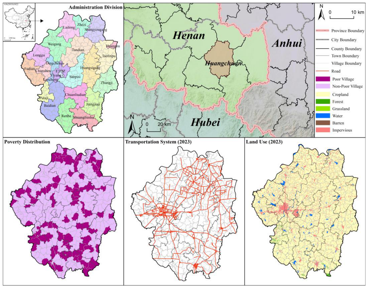
Huangchuan County is located in southeastern Henan Province and central Xinyang City (114°53′–115°21′ E, 31°52′–32°22′ N), at the junction of Hubei, Henan, and Anhui provinces, and covers an area of 1666.1 km2 (Figure 1). The terrain descends gradually from south to north, with low mountains and hills in the south and flat plains in the north (29–330 m a.s.l.). It has a transitional continental monsoon climate between the northern subtropical and warm temperate zones, with an average annual temperature of 15.7 °C, annual precipitation of 1043 mm, and a frost-free period of 239 days. Several major transport arteries intersect in the county, including the Beijing-Kowloon and Nanjing-Xi’an railways, National Highways G106 and G312, and the Shanghai-Xi’an and Daguang expressways intersect here, establishing its status as a key regional transportation hub.
As a typical agricultural county on the central plains, Huangchuan recorded per capita disposable incomes of 28,537 yuan for all residents, 36,040 yuan for urban residents, and 21,189 yuan for rural residents in 2023, all ranking first among the eight counties of Xinyang City. Its urbanization rate reached 59.39%, also topping the eight counties and exceeding the provincial average (58.08%). The urban-rural income ratio stood at 1.70, below the provincial average of 2.01, indicating balanced urban–rural development and substantial potential for spatial restructuring. The county completed its poverty alleviation mandate in 2018 and was officially removed from the national list of impoverished counties in May 2019. The study period (2013–2023) spans this critical transition from poverty alleviation to rural revitalization, providing a representative empirical basis for analyzing “driving-constraint” mechanisms. This study employs multi-source data collected through university-local collaboration research, which has been systematically cross-validated following standardized protocols to ensure objectivity and reproducibility.
The county is home to 83 poor villages, with poor populations concentrated in southern townships (>6000) and peripheral villages (>1000). The road network radiates outward from the county center along G106 and G312, forming a crisscrossed north–south and east–west trunk system, supplemented by longitudinal county roads X010 and X013. Cropland dominates land use, accounting for 86.09% of the total area in 2023, with the county center and economic development zone forming dual cores of built-up land. Water bodies (apart from the Xiaohuang River) are widely scattered across the county, while forest and grassland are concentrated in the southern low mountains and hills.

2.2. Methods

2.2.1. The Construction of Rural Network

This study takes the 303 administrative villages of Huangchuan County as uniform nodes across all rural networks. Adopting a consistent node set ensures comparability across different network layers, which provides the foundation for multilayer network analysis, but also aligns with the realities of rural governance, policy implementation, and resource allocation in China, enabling the network representation to reflect the actual institutional context of spatial restructuring. Village adjacency is defined by the sharing of a common administrative boundary.
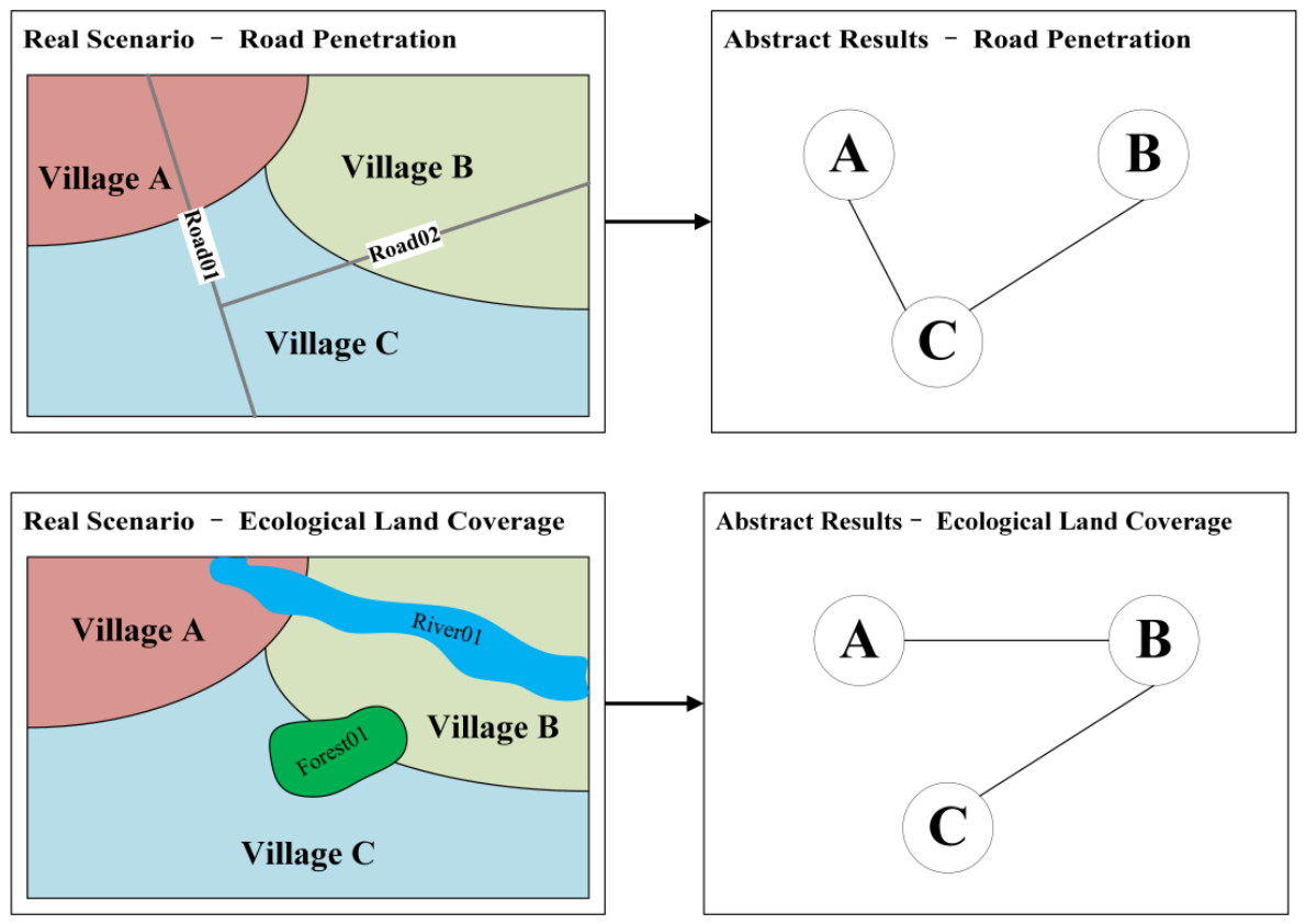
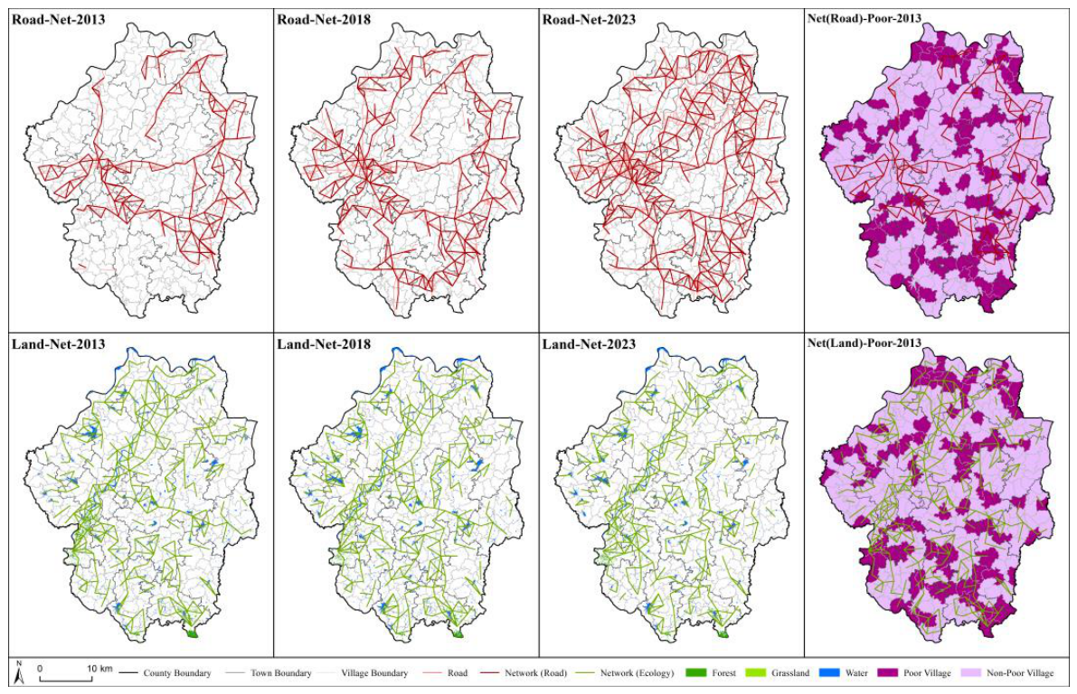
The road network is constructed to represent development drivers—namely, the role of transportation infrastructure in promoting factor flows and spatial reorganization. Using annual road data for 2013–2023, an edge is established between two spatially adjacent villages if at least one continuous road segment crosses their shared administrative boundary and extends into both village territorial polygons (Figure 2). Non-adjacent villages cannot form road edges regardless of through traffic. The network is undirected and binary (unweighted), with edges merely indicating the presence or absence of road connectivity, without distinguishing road length, travel time, or road grade.
The ecological network is constructed to represent the shaping effect of ecological constraints on spatial structure—namely, the role of ecological land patches in delimiting potential developable boundaries and shaping settlement spatial configuration. From annual land use data for 2013–2023, three ecological land use types—forest, grassland, and water bodies—are extracted. An edge is established between two adjacent villages if an ecological patch simultaneously straddles their administrative boundary (Figure 2). No minimum patch area threshold is applied; any spatial intersection (including full coverage and boundary coincidence) qualifies as a valid connection. The network is undirected and binary (unweighted), with edges indicating that two villages share the same ecological patch, rather than reflecting patch area or ecological quality differences. This approach treats ecological spaces as the fundamental skeleton of regional spatial structure—human settlements are organized around these ecological patches rather than completely eliminating them.
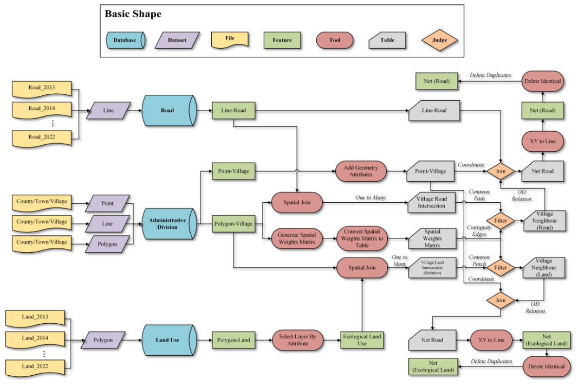
All network construction is implemented in ArcGIS (version 10.8) through the following workflow. First, village polygons are used as the core spatial unit to associate road line features and ecological land patches with individual villages. Village adjacency relationships generated based on shared boundaries are overlaid. Only pairs of adjacent villages that are connected by at least one road segment (for the road network) or share at least one ecological patch (for the ecological network) are retained to form a preliminary edge set. A standardized data cleaning step is then performed to remove duplicate edges, ensuring that only one binary edge is retained for each village pair. Since all edges are generated strictly on the premise of village adjacency defined by shared administrative boundaries, the final networks contain no topological errors such as self-loops or dangling edges. Finally, the cleaned adjacency matrices are mapped onto village nodes, generating the formal road network and ecological network (Figure 3).

2.2.2. Single Network Structure Measurement

To systematically characterize the structural features and spatiotemporal evolution patterns of the county-level single-layer road and ecological networks, five metrics are selected—node degree, structural holes, closeness centrality, clustering coefficient, and k-core—to quantitatively measure the characteristics of rural networks from five dimensions: independence, cooperation, connectivity, dependency, and stability [16,24,25]. All indicators are computed using canonical implementations by the package igraph (version 2.3.1) in R (version 4.6.0), and their mathematical definitions follow established conventions in complex network analysis. Core definitions: (1) Node degree, number of edges directly connected to a node; (2) Closeness centrality, reciprocal of average shortest path distance, with higher values indicating better accessibility; (3) Structural holes (Burt’s constraint index), higher values indicate fewer alternative paths and weaker bridging capacity; (4) Clustering coefficient, probability that two neighbors of a node are also connected; (5) K-core, maximal subgraph reflecting structural robustness.

2.2.3. Coupled Networks Synergy Measurement

To characterize the structural properties and cross-layer coupling effects of the county-level rural road–ecological multilayer network, this study builds on single-layer network metrics by developing a multilayer indicator framework that captures both intra-layer connectivity and interlayer interactions (Table 1). Owing to the computational complexity of multilayer network metrics, all calculations were implemented in R (version 4.6.0) using the muxViz (version 3.1) package [26], and all empirical results were obtained through programmatic computation.
Five multilayer network indicators were selected, including multilayer node degree, multilayer assortativity, multilayer closeness centrality, global clustering coefficient, and multilayer k-core centrality. These indicators, respectively, represent cross-layer connectivity, assortative mixing patterns, global reachability, local cohesion, and structural robustness. Furthermore, both single-layer metrics and multilayer network integration outputs are aggregated at the node level to derive network-scale macroscopic indicators. This enables a comprehensive characterization from micro-level node attributes to macro-level structural features, thus uncovering the spatial organizational patterns of structural balance, centralization, and core–periphery differentiation in county-level rural multilayer networks.

2.2.4. Evolution Mechanism Analysis by ERGM

The Exponential Random Graph Model (ERGM) is a statistical framework used to characterize the generative mechanisms of network structures [22,23], and its standard formulation is given in Equation (1):
P ( Y = y θ ) = 1 κ ( θ ) e x p θ g ( y )
where Y denotes the random graph variable representing the stochastic network; y is a specific observed network realization; θ is the vector of model parameters to be estimated, and θ denotes the transpose of the parameter vector for inner product calculation; g ( y ) is the vector of network statistics that captures endogenous structural features of the graph; κ ( θ ) = y Y e x p θ g ( y ) is the normalizing constant (i.e., partition function), which sums the exponential term over all possible network configurations y in the sample space Y to ensure the probability distribution integrates to 1.
This study employs the ergm package (version 4.12.0) in R to estimate cross-sectional static ERGMs separately for each year. The baseline model is specified as edges + gwesp (decay parameter fixed at 0.25), where the edges term controls for baseline network density, and the geometrically weighted edgewise shared partners (GWESP) term captures local and triadic closure tendencies, with its decay parameter fixed at 0.25 (Table 2). Building on this baseline, structural terms including kstar (star order set to 2) and altkstar (decay parameter fixed at 0.5) are added sequentially to capture network centralization and hierarchical differentiation. Three nodal attributes are further incorporated as covariates: village type (poor village/non-poor village, specified as nodefactor), tests for differential tie-formation preferences across village categories; population ratio and ecological land ratio (specified as nodecov) control for socioeconomic and land-use influences on tie formation. Notably, the spatial adjacency matrix is not included as a control variable in the final models. Since network edges are inherently constructed based on geographic adjacency between village units, including an explicit spatial adjacency term would introduce severe multicollinearity and endogenous bias.
Model specification is determined via a stepwise forward selection procedure, with the optimal model selected by minimizing the Akaike Information Criterion (AIC). All models are first estimated via Markov Chain Monte Carlo maximum likelihood estimation (MCMLE). If MCMLE fails to converge, maximum pseudolikelihood estimation (MPLE) is adopted as a fallback alternative. MPLE outputs are used solely to describe evolutionary trends and do not support strict statistical inference. For all MCMLE models, Geweke convergence diagnostics and goodness-of-fit (GOF) tests are performed to evaluate estimation reliability and model fit.
For the coupled network analysis, the road and ecological adjacency matrices are combined element-wise using a logical OR operation to construct a binary coupled adjacency matrix as the dependent variable. This approach produces a single-layer union projection that retains all edges from both networks, rather than a formal multiplex/multilayer ERGM specification. This choice is motivated by the inherent sparsity of county-level rural networks, as formal multilayer ERGMs would face severe convergence difficulties and unreliable parameter estimates on sparse village-level graphs. Accordingly, the coupled ERGM is interpreted descriptively as characterizing the overall structural closure of the merged road–ecological connection system. Claims regarding cross-layer interaction and synergistic effects are primarily supported by the multilayer descriptive metrics computed via muxViz, which explicitly preserve layer identity and inter-layer structure.

2.3. Data Source and Processing

This study draws on two categories of data, including geospatial datasets and statistical materials, spanning the 2013–2023 period (Table 3). The geospatial datasets include land use, administrative boundaries, and road networks. Land use data are sourced from the China Land Cover Dataset (CLCD) developed by Wuhan University, with a spatial resolution of 30 m, covering cropland, forest, grassland, water bodies, impervious surfaces, and other types. In this study, forest, grassland, and water bodies were extracted to construct the county-level ecological network. Administrative boundary data are acquired from the National Geomatics Center of China and the Tianditu Platform, and further digitized to produce county-, township-, and village-level boundary layers. Road network data were extracted from OpenStreetMap (OSM), with annual road line features used to construct the county-level road network.
The statistical materials include statistical bulletins, government work reports, and poverty alleviation documentation. Socioeconomic indicators were sourced from the Henan Statistical Yearbook and the Huangchuan County Statistical Bulletin. Lists of poor villages and poverty alleviation policy implementation records are collected from the Huangchuan County Poverty Alleviation Office and other relevant departments. Regional development strategies and policy information are derived from the Huangchuan County Government Work Reports.
All geospatial data were organized on an annual basis to ensure consistency in time-series analysis. Because the road and ecological networks constructed in this study are binary and unweighted, and focused exclusively on the presence or absence of edges, they are insensitive to continuous variations in road grades or ecological patch area. Accordingly, interannual discrepancies in OSM and CLCD data have limited impact on the core analytical conclusions, and no additional raw-data cleaning was performed beyond the standardized duplicate-edge removal step during network construction. Over the study period, the administrative boundaries of Huangchuan County remained largely unchanged, and the village nodes remained stable.

3. Results

3.1. Basic Features of Network Construction

3.1.1. Relationships Between Rural Network and County Space

The center town is located in the west-central part of Huangchuan County, and the overall spatial structure exhibits a pattern centered on the county center and expanding outward along major transportation corridors (Figure 4). The county’s transport backbone comprises four principal routes: the north–south-oriented National Highway (G106) in the west, the east–west-oriented National Highway (G312) in the central area, the southeast-extending County Road (X013) in the south, and the north–south-oriented County Road (X010) in the east, together, constitute the transportation backbone of the county.
From 2013 to 2023, the road network continuously expanded and densified along these major corridors, gradually forming a networked spatial structure radiating outward from the county center. In contrast, the ecological network is organized around the Xiaohuang River as its core ecological corridor. As a first-order tributary in the upper Huai River Basin, the Xiaohuang River traverses the central and western parts of the county and dominates the overall connectivity pattern of shared ecological patches, while the remaining ecological spaces consist of scattered lakes, forestlands, and grasslands. Over the 2013–2023 period, the overall ecological network structure remained relatively stable, with only a slight decline in local network density.
Spatial overlay analysis of poor village distribution further reveals that poor villages exhibit high spatial overlap with the ecological network but a clear spatial mismatch with the road network, indicating that poor villages are mainly concentrated in areas characterized by stronger ecological constraints and weaker transportation accessibility. The spatial allocation of poverty alleviation projects further validates the above spatial pattern. The period 2015–2018 marked a critical phase in Huangchuan County’s poverty alleviation efforts, during which a total of 585 poverty alleviation projects were implemented, with the share of infrastructure projects increasing from 0% in 2015 to 91.6% in 2018, representing a total investment of 164 million yuan. These infrastructure projects were predominantly concentrated in townships with larger poor populations in the southern part of the county, which tend to lie within the ecological zones while being separated from major transportation corridors. Compared with conventional spatial description, network-based overlay analysis yields additional insights, demonstrating the analytical value of a network perspective for county-level spatial research.

3.1.2. Variation in Network Connections

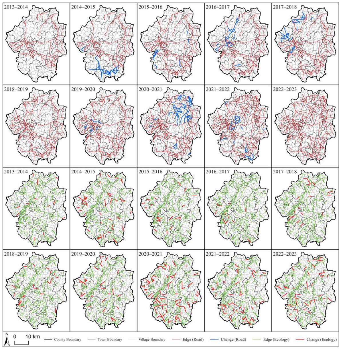
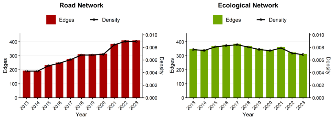
The number of nodes in rural networks remained stable between 2013 and 2023, but edge counts exhibited markedly different evolutionary trajectories across road and ecological networks (Figure 5 and Figure 6). These results indicate that the spatial restructuring of the county was mainly reflected in the reconfiguration of inter-village connection intensity and patterns, rather than the expansion of the node scale.
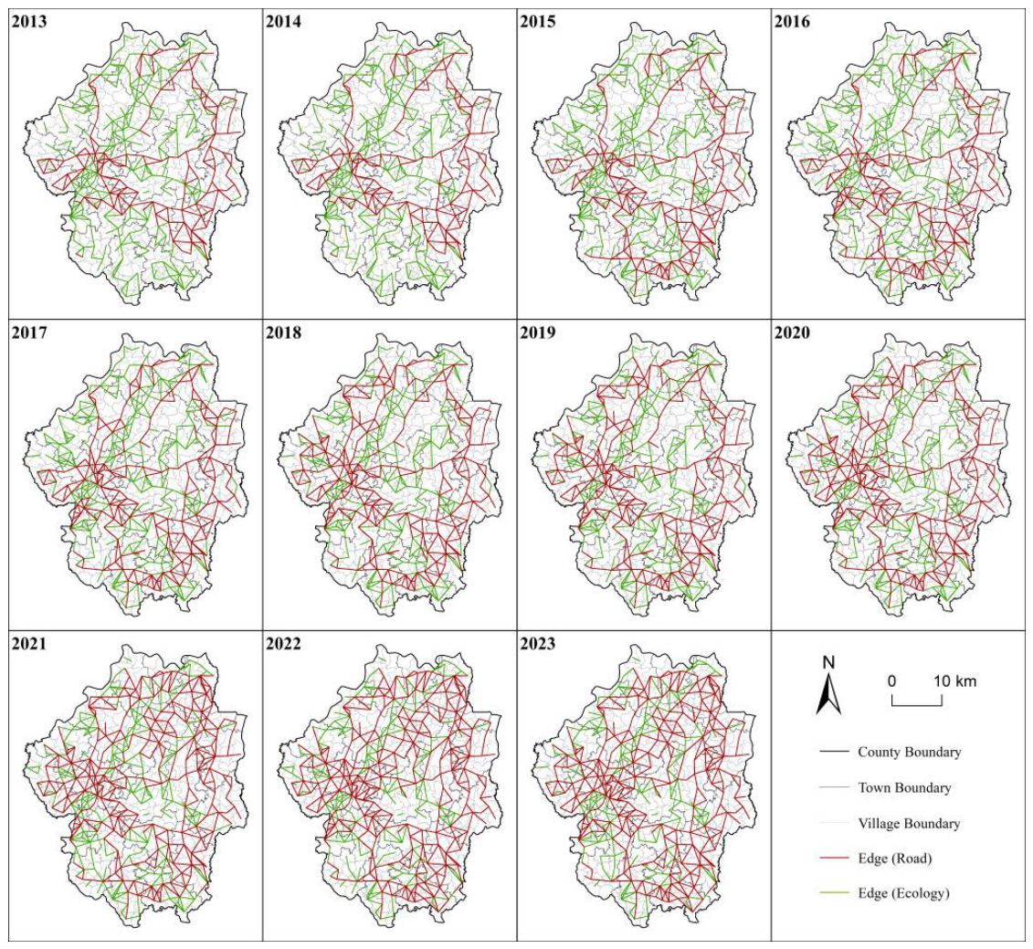
The road network underwent continuous expansion. The number of edges rose from 194 in 2013 to 410 in 2023, equivalent to an average annual increase of 21.6 edges. Network density increased from 0.0042 to 0.0090, representing a 114.3% rise and markedly enhancing overall connectivity (Figure 5). Newly added road edges were primarily distributed in weakly connected areas (Figure 6). These changes are attributable to two driving forces: policy prioritized transportation investment in impoverished regions during poverty alleviation, and sustained local investment support. From 2013 to 2023, the county’s fixed asset investment increased from 15.60 billion yuan to 39.66 billion yuan, providing strong financial support for the continuous improvement of transportation infrastructure. Over the same period, highway freight volume increased from 8.42 million tons to 10.41 million tons, and passenger volume grew from 12.09 million to 14.29 million persons, which may be partly attributable to improved road connectivity. The core road network backbone took shape around 2019 and stabilized by 2021. This evolutionary trajectory is temporally consistent with the timeline of poverty alleviation efforts, suggesting a potential policy-driven influence.
By contrast, the ecological network contracted slightly. The edge count decreased from 350 to 314, corresponding to an average annual reduction of 3.3 edges. Network density dropped from 0.0076 to 0.0069, representing a 9.2% decline (Figure 5). The overall ecological pattern remained intact, and only scattered local connections were reduced while the core spatial corridors of ecological land remained spatially continuous (Figure 6). This change is consistent with the expected outcomes of land consolidation and ecological pattern optimization.
Overall, the rural network evolution in Huangchuan exhibits two core characteristics: rapid expansion of road networks and steady optimization of ecological networks. This pattern is consistent with a spatial evolution process in which transportation connectivity expands while the overall configuration of ecological land remains relatively stable.

3.1.3. Spatial Pattern of Coupled Networks

Spatial overlay analysis clearly depicts the evolutionary patterns of coupling and spatial interaction between the two networks (Figure 7). The road-ecological coupling network in Huangchuan County shows an evolutionary trend from relative independence to limited intersection. In 2013, the two networks remained largely separated. The road network concentrated in the county center and along trunk lines, while the ecological network was distributed along the Xiaohuang River corridor and scattered ecological patches. As the road network has densified across the county, partial intersection and integration gradually emerged at county peripheries and ecological transition zones.
This localized integration is clearly exemplified in three southern townships—Renhe, Shuangliushu, and Baidian—where the spatial distribution of poverty alleviation infrastructure projects overlaps with both the expanding road network and concentrated ecological land uses. Improved road connectivity may have provided enabling conditions for the development of local characteristic industries. In Renhe Town, improved transportation facilitated the development of the flower and nursery industry (approximately 300 ha, providing more than 200 jobs) and tea cultivation (approximately 200 ha, benefiting more than 3000 households). Shuangliushu Town promoted chili pepper cultivation (over 20 ha) and planned a full-value-chain processing system. Baidian Town developed chrysanthemum deep-processing (with a 2000 m2 processing facility employing over 200 people) and fruit and forest industries. The spatial trajectory of this industrial expansion closely aligns with the extension of the road network into the historically under-connected southern areas. This spatial pattern is consistent with a potential virtuous cycle, in which transport improvements support the conversion of ecological resources into livelihood and economic value.
Overall, spatial exclusion still dominates the coupling relationship. Despite a 114.3% growth of road network density over the decade, core ecological corridors and key ecological functional areas have not been extensively encroached. Spatial overlay shows that road construction rarely encroaches on core ecological patches, which aligns with ecological protection requirements. The aforementioned characteristic industries are precisely located in ecological transition zones rather than core ecological areas, achieving spatial compatibility between industrial development and ecological protection. This persistent spatial separation aligns with the prioritization of ecological conservation in the region. It indicates that Huangchuan County adheres to the ecological security baseline during rural development and transportation construction, thereby preserving the overall spatial configuration of ecological land.

3.2. Structural Measurement of Networks

3.2.1. Structural Metrics of Road Networks

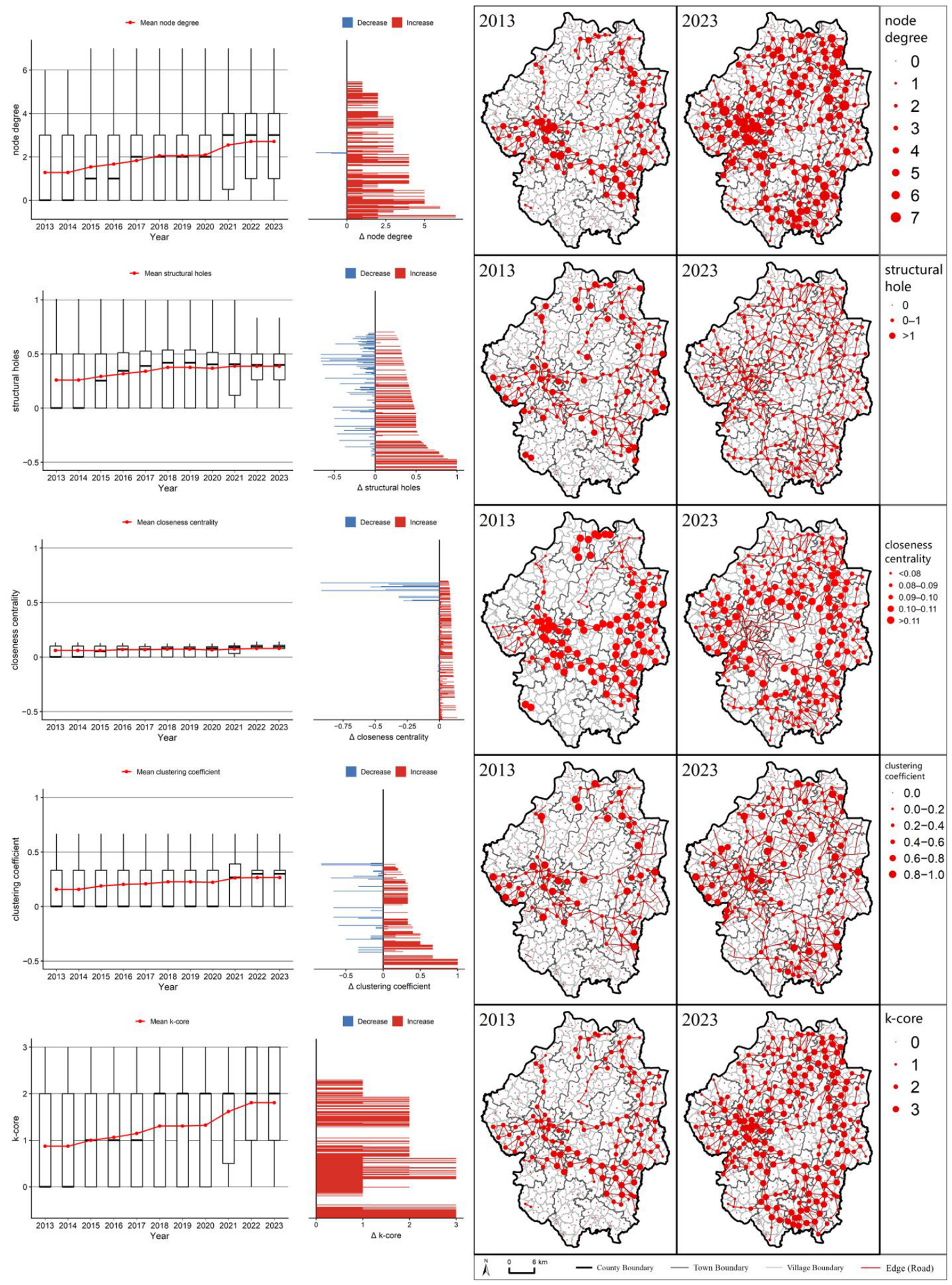
Overall connectivity of the road network in Huangchuan County improved significantly, accompanied by intensified internal hierarchical differentiation (Figure 8). Mean node degree increased from 1.28 in 2013 to 2.71 in 2023, representing a 111.7% rise; average k-core values grew from 0.87 to 1.81 (a 108.0% increase), reflecting the continuous strengthening of the network’s core skeleton. The structural holes constraint index increased from 0.259 to 0.386 (up 49.0%), with its median value rising from 0 to 0.398, which indicates enhanced network closure and stability. The clustering coefficient increased from 0.157 to 0.266 (up 69.4%), suggesting a strengthening trend of local agglomeration. The mean closeness centrality increased from 0.060 to 0.079, while its standard deviation narrowed from 0.115 to 0.045, reflecting improved overall accessibility and reduced disparities among nodes. Overall, the road network achieved comprehensive enhancement in connectivity, core dominance, and local agglomeration, evolving from a loose and disordered state to a well-defined core–periphery hierarchical structure.
The spatial pattern of the road network evolved from core agglomeration to county-wide linkage (Figure 8). The number of nodes with high degree values increased substantially, with their spatial distribution expanding from the county core to peripheral townships, and high-value nodes formed a multi-center coordinated hub pattern in the central region. The number of high k-core villages increased from 18 in 2013 to 123 in 2023, with stable connection coverage expanding southward and eastward from the county periphery. High clustering coefficient nodes spread from the central region toward the eastern periphery, reflecting the radiation of local agglomeration from the core outward.
The connectivity gap between the county center and peripheral townships continued to narrow, indicating marked improvement in spatial balance. Notably, during 2021–2023, the mean node degree increased from 2.54 to 2.71 and the mean k-core from 1.61 to 1.81, indicating rapid reinforcement of the network skeleton during the final phase of poverty alleviation. This evolutionary trajectory aligns with the policy direction of extending transportation infrastructure and core functions toward rural areas. However, the maximum closeness centrality in 2023 was only 0.142, well below the theoretical maximum of 1, with a standard deviation of 0.045, suggesting that accessibility in remote villages remains inadequate and that structural deficiencies persist in the peripheral segments of the road network.

3.2.2. Structural Metrics of Ecological Networks

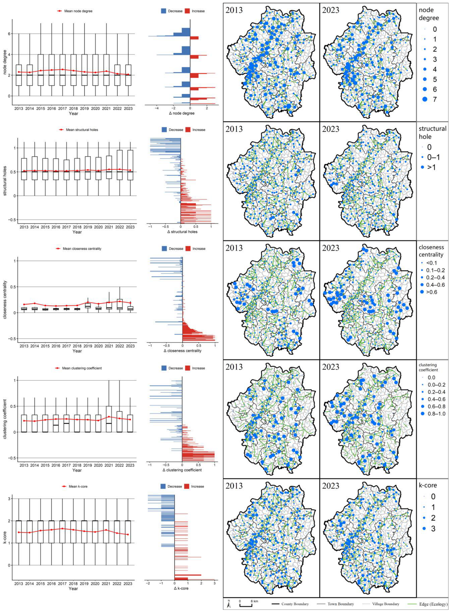
The ecological network in Huangchuan County remained largely stable with only minor local structural adjustments, standing in sharp contrast to the rapid expansion of the road network (Figure 9). From 2013 to 2023, the mean values of major indicators generally fluctuated, rising first and then declining or leveling off. Mean node degree decreased from 2.31 to 2.07 (−10.3%), and mean k-core from 1.48 to 1.38 (−6.7%), both peaking around 2017 before gradually declining. The structural holes constraint index fluctuated slightly between 0.52 and 0.55, remaining generally stable. The mean clustering coefficient increased from 0.218 to 0.243 (+11.5%), but the median remained 0 in most years, indicating that while local agglomeration showed a slight strengthening trend, the overall clustering level remained low. Mean closeness centrality increased from 0.160 to 0.188 (+17.5%), with its standard deviation widening from 0.255 to 0.293, indicating improved accessibility for a subset of nodes alongside growing inter-node disparities.
As the fundamental skeleton of regional spatial structure, the ecological network features highly stable core corridors and major ecological patches, a pattern consistent with the stringent protection requirement of ecological red lines and conservation policies. This explains the overall stability of indicators characterizing core structures, such as node degree and k-core. Meanwhile, the increases in clustering coefficient and closeness centrality reflect enhanced connectivity among local ecological patches and improved structural integration, while the widening standard deviation suggests that these improvements have been concentrated in core areas and their peripheries, with limited progress in remote areas.
Spatially, villages with high node degree values were distributed along the Xiaohuang River core corridor and increasingly concentrated in the southwest. Nodes with high clustering coefficient expanded from the south-central region toward the northwest, while high-k-core nodes extended from the western core area southward and eastward, forming a multi-level pattern with one primary core, giving rise to a hierarchical structure consisting of one primary core and multiple secondary cores. Although the gap between core and peripheral areas has narrowed somewhat, ecological patch adjacency in remote villages remains weak. Overall, structural stability does not equate to balanced functional performance across the network.

3.2.3. Structural Metrics of Coupled Networks

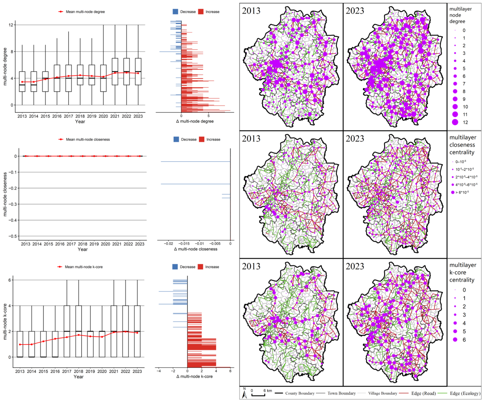
The multilayer metrics of the coupled network capture the synergistic evolutionary dynamics between the road network as the dominant driving force and the ecological network as the foundational constraining factor (Figure 10). From 2013 to 2023, the mean multilayer degree increased from 3.45 to 4.75 (+37.5%), and the mean multilayer k-core increased from 0.98 to 1.89 (+93.3%), both showing sustained growth that indicates simultaneous enhancement of connectivity and core skeleton of the coupled network. Multilayer closeness remained on the order of 10−5 with minimal variation, suggesting that the coupled network has not yet developed an efficient county-wide connectivity system.
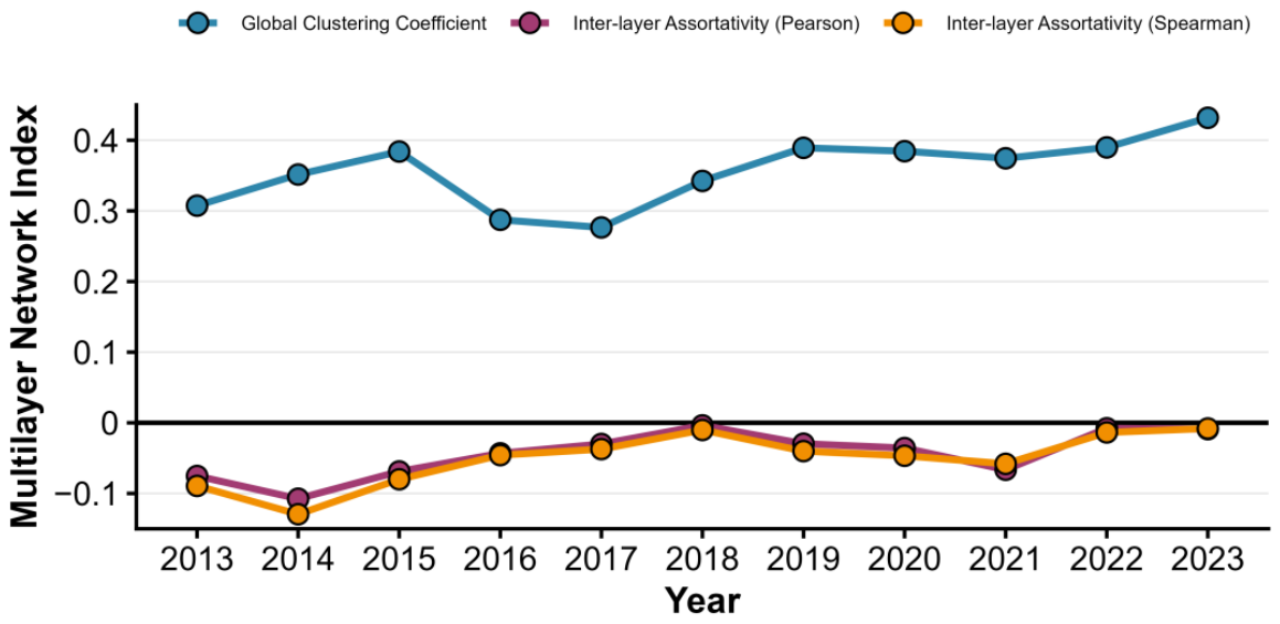
Interlayer assortativity remained consistently negative (ranging from −0.075 to −0.009), indicating persistent spatial exclusion between the two networks at the node level. Its absolute value declined steadily over the period, pointing to weakening exclusion and gradually enhanced coordination (Figure 11). The multilayer global clustering coefficient increased from 0.307 to 0.432 (+40.7%), reflecting a tendency toward tighter overall structure and improved local coordination in the coupled network. Statistical tests further confirmed these trends: the absolute value of interlayer assortativity was significantly negatively correlated with year (Pearson’s r = −0.661, p < 0.05), and the multilayer global clustering coefficient was significantly positively correlated with year (Pearson’s r = 0.612, p < 0.05). This pattern is consistent with an evolutionary shift from predominant spatial exclusion to limited local integration.
The spatial pattern of the coupled network has evolved from core-dominated polarization to county-wide coordinated development (Figure 10). Nodes with high multilayer degree were mainly concentrated in and around the county center of Huangchuan, gradually expanding to peripheral townships, forming a multi-center spatial structure with the county center as the primary core and towns in the northeastern and southern regions as secondary cores. High multilayer k-core nodes were predominantly distributed in overlapping core areas of road and ecological networks, expanding from the Xiaohuang River corridor in the early period toward the southern and eastern parts of the county, broadly consistent with the southward expansion trend of single-layer road k-core, suggesting that the core skeleton of the coupled network is mainly driven by the expansion of the road network.
The gap in coupling intensity between the county center and peripheral areas continued to narrow, with the outward expansion of the road network and the foundational support of the ecological network jointly promoting the formation of a county-wide coordinated pattern. Nevertheless, coupling weaknesses persist in some remote villages, where multilayer degree and multilayer k-core values were significantly below the county averages, reflecting the dual constraints of insufficient road penetration and weak ecological patch connectivity. Overall, this pattern suggests that the spatial evolution of the coupled network is driven both by road expansion and constrained by the spatial configuration of ecological land. These two forces jointly shape a coupled structure defined by a dense core and a sparse periphery.

3.3. Analysis of Network Evolution Mechanisms

3.3.1. Evolution Mechanism of Road Networks

ERGM estimation results of the road network are summarized in Table 4. Owing to limited inter-village road coverage and overall sparse network structure in the early stage, models for 2013–2016 were estimated using MPLE, for which MCMC convergence diagnostics and goodness-of-fit tests are not applicable; their results are only used to reflect evolutionary trends. Models for 2017–2023 adopt MCMLE estimation. The joint p-values of Geweke tests and minimum p-values of GOF tests all exceed 0.05, indicating satisfactory convergence, good model fit, and reliable estimation outputs. Statistical inferences in this section are drawn primarily from the 2017–2023 MCMLE outputs, while 2013–2016 MPLE results serve as descriptive references for early-stage evolutionary trends.
The Edges term is significantly negative at the 0.1% level across 2017–2023, confirming that the county-level road network exhibits the typical sparsity of spatial networks, with a baseline edge probability far lower than that of equivalent random networks. Temporally, the absolute value of its coefficient generally declines from 6.286 in 2017 to 5.688 in 2023, aligning with the expectation that sustained transport infrastructure investment has steadily raised baseline density. The results in 2013–2016 show the same downward trend in the absolute value of the Edges coefficient, decreasing from 6.623 to 6.077 over the period, which aligns with the later evolutionary trajectory and together demonstrates a sustained increase in road network density.
The GWESP term is significantly positive at the 0.1% level in 2017–2023, with its coefficient remaining stable within the range of 2.45–2.50. This points to a strong and persistent triadic closure effect in the road network: two villages sharing a common neighboring village are more likely to form a direct road connection, reflecting that the network has formed a closed mesh structure with intensified local agglomeration. The results in 2013–2016 show that the GWESP coefficient rose steadily from 2.088 to 2.268 in the early stage, indicating that the triadic closure effect strengthened gradually before stabilizing, in line with the upward trend of clustering coefficients observed in the descriptive network analysis.
In terms of network hierarchical structure, Kstar2 is significantly negative throughout the 2017–2023 period, with the absolute value of its coefficient expanding continuously. This indicates that network centralization gradually declines and a polycentric equalization trend emerges. Altkstar remains statistically insignificant in this period, suggesting that high-degree hierarchical differentiation has weakened substantially in the mature network stage. For the 2013–2016 period, by contrast, Kstar2 lacks statistical significance while Altkstar is significantly positive, indicating obvious high-degree hierarchical differentiation and a dominant monocentric radial pattern in the initial network. Together, the two stages trace the complete evolutionary path of the road network, shifting from a monocentric radial pattern to a balanced polycentric pattern.
For nodal attributes, the results in 2017–2023 show that the coefficient for poor village status is significantly negative during 2017–2020 and becomes statistically insignificant again after 2021. It suggests that poor villages had lower probabilities of road connections during the critical poverty alleviation period, and the gap in road construction between poor and non-poor villages narrowed as equalization improved following the completion of poverty alleviation. The population ratio coefficient remains positive and highly significant after 2017, with an overall upward trend, which indicates that the population agglomeration’s pulling effect on road layout strengthens as the network develops. The ecological land ratio coefficient is significantly negative across all years, exerting a stronger constraining effect in the early stage and remaining significant despite fluctuations afterward. The results in 2013–2016 are consistent with this long-term constraint pattern, while the coefficients of poor village status and population ratio do not reach statistical significance in the early sparse-network stage.
Overall, the evolution of county road networks is defined by three core features: rising density, structural closure, and hierarchical flattening. Transportation infrastructure construction continuously increases network density, the triadic closure effect transforms the network from a linear skeleton into a meshed structure, and declining network centralization and hierarchical differentiation drive the shift toward a balanced polycentric pattern. The pulling force of population agglomeration and the restriction of ecological spaces coexist with varying intensities over network development, jointly shaping the spatiotemporal evolutionary trajectory of county road networks.

3.3.2. Evolution Mechanism of Ecological Networks

ERGM estimation results of the ecological network are summarized in Table 5. All models across years are estimated via MCMLE. The minimum p-value of the Geweke convergence test for 2014 is 0.034, falling slightly below the 0.05 threshold and indicating relatively weak convergence. Accordingly, the 2014 estimation should be interpreted with caution and serves as a descriptive reference rather than a basis for strict statistical inference. Models for other years achieve favorable convergence and fitting performance and can accurately reproduce the structural characteristics of the real ecological network.
The Edges term is significantly negative at the 0.1% level for all years, confirming that the county-level ecological network also features typical sparse spatial characteristics, with a far lower baseline probability of inter-village edges formed by shared ecological patches than random networks. Temporally, the coefficient fluctuates slightly within the range of 5.2–5.7 in absolute value without a continuous downward trend, revealing a relatively stable pattern of ecological land and minor overall changes in the density of inter-village ecological patch connections.
The GWESP term is significantly positive at the 0.1% level in all years. Its coefficient rises slowly from 1.954 in 2013 to a peak of 2.294 in 2021, followed by a mild decline afterward. This identifies a stable triadic closure effect in the ecological network: two villages sharing one ecological patch are more likely to form indirect connections via other ecological patches. This effect strengthens over time, reflecting a trend toward contiguous clustering of ecological patches at the county scale, alongside continuously improved adjacency integrity of local ecological spaces.
In terms of network hierarchical structure, the Kstar2 term is significantly negative at the 0.1% level for all years. The absolute value of its coefficient expands first and then shrinks, peaking at 0.219 in 2021. This suggests low overall centralization of the ecological network; ecological patch connections do not concentrate in a small number of core villages and show a balanced distribution pattern. The equalization trend intensifies continuously from 2013 to 2021 and weakens slightly in later years. The Altkstar term is statistically insignificant across all years, which means the county ecological network has no obvious high-degree hierarchical differentiation and maintains a flat overall structure without a hierarchical pattern dominated by a small number of super-core nodes.
Regarding nodal attributes, the coefficient of poor village status is statistically insignificant in all years, indicating that village poverty status exerts no significant impact on the formation of inter-village ecological patch connections, and the spatial distribution of the ecological network is not systematically shaped by village poverty types. The population ratio coefficient is significantly positive for all years, implying that villages with larger population sizes are more likely to form shared ecological patch connections with neighboring villages. This is largely because more populous villages generally cover wider geographic areas and contain more cross-village ecological patches. The ecological land ratio term does not reach statistical significance in any study year, which reflects that inter-village ecological patch connections are primarily determined by the distribution of continuous ecological patches across administrative boundaries, rather than the proportion of ecological land within a single village.
Overall, the county-level ecological network is characterized by three core features: overall stability, local closure, and flat hierarchy. The overall network density remains stable, the gradually strengthened triadic closure effect drives the contiguous distribution of local ecological patches, and the hierarchical structure stays balanced and flat throughout the study period. The evolution of the ecological network is mainly dominated by the spatial distribution pattern of natural ecological spaces, with population size exerting only limited positive effects, while village poverty status and internal ecological land proportion have no significant impacts.

3.3.3. Evolution Mechanism of Coupled Networks

ERGM estimation results of the coupled network are summarized in Table 6. All models for each year are estimated via MCMLE. Except for 2017, 2020, and 2023, in which the joint p-values of Geweke tests are close to the critical threshold, models for other years achieve favorable convergence and fitting performance and can effectively reproduce the structural features of the merged network.
The Edges term is significantly negative at the 0.1% level across all years, confirming that the road-ecology coupled network retains the typical sparsity of spatial networks, with a baseline probability of inter-village edges formed by shared road or ecological links far lower than that of equivalent random networks. The absolute value of the coefficient shows a slight overall downward trend, declining from 4.908 in 2013 to 4.659 in 2023. This reveals that with the continuous expansion of road networks and gradual contiguous distribution of ecological patches, the baseline density of inter-village coupled connections rises steadily, and the connectivity scope of the merged network keeps expanding.
The GWESP term is significantly positive at the 0.1% level for all years. Its coefficient rises continuously from 2.180 in 2013 to a peak of 3.004 in 2021, followed by a mild decline, with an obvious overall growth range. This points to a strong triadic closure effect in the coupled network: two villages sharing one neighboring village are more likely to form direct coupled connections. This effect strengthens over time, reflecting that after the superposition of road and ecological links, the degree of local agglomeration and structural closure of the merged network keeps increasing, and the whole network evolves from scattered linear structures to contiguous mesh structures. Importantly, this closure effect is a structural outcome of the superposition of two link types and cannot be interpreted as direct evidence of cross-layer interaction mechanisms between road and ecological networks.
In terms of network hierarchical structure, the Kstar2 term is significantly negative at the 0.1% level in all years. The absolute value of its coefficient expands first and then shrinks, peaking at 0.303 in 2021. This means the coupled network has low overall centralization; connections do not concentrate on a small number of core villages and present a balanced distribution pattern, with the most prominent equalization trend emerging in the middle of the study period. The Altkstar term is statistically insignificant across all years, which indicates that the coupled network has no obvious high-degree hierarchical differentiation, maintains a flat overall structure, and fails to form a hierarchical pattern dominated by a small number of super-core nodes.
Regarding nodal attributes, the coefficient of poor village status is statistically insignificant in all years, indicating that village poverty status exerts no systematic impact on the formation of coupled connections. The population ratio coefficient is significantly positive at the 0.1% level for all years and presents an overall fluctuating upward trend, which implies that villages with larger population sizes have higher probabilities of forming coupled connections, and the positive pulling effect of population agglomeration on the layout of the merged network persists throughout the period. The ecological land ratio term shows no statistical significance from 2013 to 2014, but becomes significantly negative from 2015 onward, with continuously expanding absolute coefficient values and growing negative restrictive effects. It reflects that the restraining effect of ecological spaces on the coupled network gradually becomes prominent, and the pattern of ecological land constitutes a key restrictive factor shaping the structure of the merged network.
Overall, the road-ecology coupled network is defined by three core evolutionary features: steadily rising density, continuously strengthened closure effect, and balanced flat structure. The triadic closure degree of the merged network is higher than that of single-layer networks, which mainly stems from the structural superposition effect of two types of links rather than the mechanistic evidence of cross-layer synergy. The evolution of the coupled network is associated with both the positive effect of population agglomeration and the negative effect of ecological land proportion, both of which show strengthening trends over time.

4. Discussion

This study develops a road-ecology coupled network framework and integrates multilayer network analysis with the Exponential Random Graph Model (ERGM) to unpack the evolutionary characteristics and formation mechanism of county spatial structure in Huangchuan County from 2013 to 2023. The discussion is structured around three core themes.

4.1. Methodological Limitations and Implications for Result Interpretation

This study integrates the two types of networks into a unified village-level node system and builds a comparable, couplable dual-network framework. Nevertheless, four limitations exist and call for prudent interpretation of the results.
First, a scale mismatch exists in node attributes. Socio-economic covariates including population and land use are incorporated into the ERGM analysis, and nodal covariates such as population ratio and ecological land ratio show statistically significant effects in most years, but their explanatory power is notably weaker than endogenous structural terms, and effect sizes fluctuate substantially across years. This represents a common dilemma in rural network research: village-level statistical data are limited, and inter-village heterogeneity is prominent [19]. Administrative villages in Huangchuan County vary drastically in territorial scale and population size, and the average value at the village unit cannot accurately characterize node attributes [27]. Therefore, the findings mainly reflect the endogenous structural effects of the network, while the impacts of exogenous socio-economic attributes may be underestimated [28].
Second, OSM data have temporal validity deviations. The annual completeness of historical road data fluctuates with mapping activities [29]. This study adopts a binary unweighted network that only focuses on the presence of connectivity. Although this design reduces interference from data discrepancies, missing mapping records of low-grade roads in the early years may still lead to a slight overestimation of the 10-year expansion magnitude of the road network. Official road mileage statistics were not available for full quantitative validation in this study, and the growth trend should be interpreted with appropriate caution.
Third, the binary network design entails simplification and trade-offs. Continuous indicators such as road length, travel time, and ecological patch area are excluded from the study, which aligns with the practical logic of rural space that connectivity matters more than traffic quality [30,31]. Accordingly, the conclusions apply to structural analysis at the level of connectivity presence, rather than refined assessment of connectivity quality.
Fourth, the ERGM estimation has inherent constraints. For the road network, models for 2013–2016 are estimated via maximum pseudolikelihood estimation (MPLE) due to network sparsity, and these results are used only for trend reference rather than strict inference. For the ecological network, the 2014 model shows weak convergence and requires cautious interpretation. For the coupled network, the 2017, 2020, and 2023 models have Geweke p-values near the 0.05 threshold, indicating relatively weak convergence. More critically, the coupled ERGM is based on a logical OR union projection that discards layer identity and cannot identify cross-layer causal interactions between road and ecological ties. All claims regarding cross-layer synergy are therefore grounded in the multilayer descriptive metrics, which explicitly preserve layer identity and inter-layer structure. The union-projection ERGM serves only to characterize the overall structural closure of the merged connection system.

4.2. Theoretical Dialogue of Core Findings

The transformation of the road network from a monocentric centralized structure to a polycentric balanced structure is consistent with the theoretical expectation that infrastructure guides spatial equalization. The coordinated changes in the Edges, GWESP, and Star coefficients form a supportive evidence chain for structural transformation. The study further reveals the internal mechanism of this transformation: rising network density enhances transitivity, which in turn erodes the centralized advantage of the single core. From the perspective of infrastructure resilience theory, a polycentric structure confers greater anti-interference capacity and structural robustness [32]. Transportation investment during the poverty alleviation campaign not only expanded the road network in scale but also reshaped the resilience foundation of the network structurally.
The ecological network features a “stable backbone with localized fine-tuning”, aligning with the spatial logic of coexisting rigid constraints and flexible optimization [33]. Its Edges coefficient fluctuates steadily in the absolute range of 5.2–5.7 with no sustained trend, indicating stable overall connection density and rigid protection of core ecological spaces. The GWESP coefficient rises gradually to a peak in 2021 before a slight decline, reflecting a trend of local ecological patches becoming contiguous and clustered [34]. In terms of hierarchical characteristics, the consistently significant negative Kstar2 and insignificant Altkstar across all years indicate that the ecological network maintains a flat, balanced spatial structure without dominant super-core villages. As noted previously, only the 2014 model shows weak convergence, requiring cautious interpretation.
From an interpretive perspective, the spatial pattern of poor villages—“adjacent to ecological spaces but remote from transportation”—reflects a potential structural mismatch between development opportunities and environmental constraints [35]. Poor villages cluster in areas covered by the ecological network yet outside the road network, forming a spatial overlap of ecological endowment and concentrated poverty [36]. This configuration is consistent with broader findings on rural infrastructure vulnerability, where marginalized settlements often bear disproportionate environmental risks while remaining underserved by transport networks [37]. This exploratory observation echoes the theoretical concerns of environmental justice [38] and points to a distinctive lock-in effect: rich ecological resources cannot be converted into development momentum due to insufficient traffic accessibility [39,40]. Rather than functioning solely as a transportation facility, infrastructure acts as a spatial mediator that determines whether ecological assets can be transformed into livelihood opportunities. Viewed through the lens of environmental justice, this imbalance raises critical questions about the equitable distribution of accessibility and ecological burdens [41]. Consequently, the coexistence of ecological abundance and transportation deprivation may constitute a form of spatial injustice, whereby villages bearing greater ecological conservation responsibilities receive disproportionately limited accessibility and development opportunities [42]. Notably, the foregoing discussion of spatial justice is an interpretive extension derived from network structure findings and does not represent a statistically tested conclusion of this study.
For the coupled network, the continuous decline in the absolute value of interlayer assortativity and the steady rise in the multilayer global clustering coefficient jointly indicate a shift from predominant spatial exclusion to limited local integration. This pattern is consistent with findings from other road-ecology network studies, which have documented systematic spatial tensions between road expansion and ecological land configuration [6]. However, the union-projection ERGM results only reflect enhanced structural closure of the merged network and cannot be directly interpreted as evidence of cross-layer synergistic mechanisms. The observed coordination trend therefore remains at the level of spatial pattern association, and the causal interaction between road expansion and ecological conservation requires further verification with formal multilayer network models that explicitly preserve layer identity and inter-layer dependencies.

4.3. Socio-Ecological Implications

The evolution of county spatial structure is a dynamic balancing process between development drivers and ecological constraints. In the coupled network, road expansion and ecological constraints operate in a dynamic interplay of mutual adjustment, and multilayer descriptive metrics are consistent with a trend of strengthened local clustering across the two network layers over the study period. This indicates that county planning may explore collaborative paths based on the structural interaction between the two, rather than pitting development against protection.
The resource curse effect facing poor villages underscores the need for differentiated policy responses. Areas with rich ecological resources but weak transportation bear dual constraints of priority protection and insufficient investment, forming a locked development chain. Network-based governance can act as an institutional tool to break this dilemma.
The coupled network framework provides an operable quantitative analysis tool for county-level spatial planning. Integrating development drivers and ecological constraints into a unified analytical system makes the evolution of spatial structure measurable, comparable, and interpretable. The framework can also simulate structural changes under different policy scenarios, providing quantitative evidence to support planning optimization.

5. Conclusions

Taking Huangchuan County as the research case, this study develops a road-ecology coupled network analysis framework and applies complex network indicators, multilayer network analysis, and ERGM to examine the evolutionary characteristics and underlying formation mechanisms of county spatial structure over the 2013–2023 period. Three research hypotheses are empirically tested, receiving varying degrees of support.
The first hypothesis that road and ecological networks evolve from mutual exclusion to interweaving receives partial support. Interlayer assortativity remains consistently negative, indicating that the overall pattern of spatial exclusion has not been fundamentally reversed. Yet its absolute value keeps decreasing, and localized interweaving of roads and ecological land has emerged in southern townships. The second hypothesis that the elite capture effect sustains the advantage of core nodes is not supported. The Star coefficient shifts from positive to negative, and network concentration keeps declining, suggesting that large-scale transportation investment during the poverty alleviation campaign has eroded the dominant position advantage of core nodes. The third hypothesis that the poverty alleviation strategy triggers leapfrog spatial changes is partially supported. The road network presents obvious discontinuous expansion during the concentrated implementation of poverty alleviation infrastructure projects, matching the policy timeline. In contrast, the ecological network is restricted by rigid ecological redline constraints and only undergoes mild local adjustment throughout the whole period, without any leapfrog structural transformation in any single year.
Three core conclusions can be drawn from this study. First, the road network has undergone a marked structural transition from a monocentric centralized mode to a polycentric balanced mode, with transportation investment driving both scale expansion and structural optimization. Second, the ecological network follows an evolution trend of a stable backbone with localized fine-tuning: the core spatial pattern of ecological land remains intact, local patch adjacency keeps improving, but edge areas are still relatively weak. The coupled network features weakened spatial exclusion and structural flattening under the balance of drivers and constraints, forming a polycentric collaborative coupling pattern. Notably, cross-layer association evidence is primarily supported by multilayer network metrics, while the union-projection ERGM only reflects the overall structural closure of the merged network. The spatial pattern of poor villages adjacent to ecology and remote from transportation is consistent with the structural mismatch between development opportunities and environmental constraints, which is a key spatial issue to address in the post-poverty alleviation era.
Constrained by the scale heterogeneity of village-level socioeconomic data, the explanatory power of exogenous nodal attributes in ERGM models is limited compared with endogenous structural effects. In addition, the coupled ERGM based on union projection has weak convergence in individual years and cannot directly identify cross-layer causal mechanisms, which restricts the depth of mechanism interpretation. Future research can be expanded in multiple directions: more fine-grained village-level socio-economic data can be collected through in-depth field surveys; multilayer and temporal exponential random graph models can be introduced to capture the dynamic interaction mechanism of coupled networks; and multi-county comparative studies can be conducted to test the applicability and generalizability of the proposed framework.

Supplementary Materials

The following supporting information can be downloaded at: https://www.mdpi.com/article/10.3390/su18147065/s1, File S1: minimal dataset.

Author Contributions

Conceptualization, C.Y. (Chao Yu) and J.G.; methodology, C.Y. (Chao Yu), C.Y. (Chenao Yang) and Z.Z.; investigation, C.Y. (Chenao Yang), Z.Z., Y.L., C.H., Y.F. and J.W.; resources, C.Y. (Chenao Yang), Z.Z., Y.L., C.H., Y.F. and J.W.; writing—original draft preparation, C.Y. (Chao Yu) and C.Y. (Chenao Yang); writing—review and editing, Z.Z., Y.L., Y.F. and J.W.; visualization, C.Y. (Chao Yu), C.Y. (Chenao Yang) and Z.Z. All authors have read and agreed to the published version of the manuscript.

Funding

This research was funded by the National Natural Science Foundation of China (42371225); the Social Science Fund of Henan Province (2023BSH021); the Key R&D and Promotion Project (Soft Science Research) in Henan Province (242400410100); the Postgraduate Research and Innovation Fund of Xinyang Normal University (2025KYJJ83).

Institutional Review Board Statement

Not applicable.

Informed Consent Statement

Not applicable.

Data Availability Statement

The data used in this study are derived from publicly available sources. (1) Road data are derived from OpenStreetMap [https://www.openstreetmap.org (accessed on 2 May 2026)]; (2) Land use data are obtained from the CLCD dataset [https://zenodo.org/records/18180184 (accessed on 2 May 2026)]; (3) Administrative division data are redrawn based on the public version of fundamental geographic information data [https://cloudcenter.tianditu.gov.cn/dataSource (accessed on 2 May 2026)] and the paper maps provided by Huangchuan County; (4) Socioeconomic data are sourced from the Henan Provincial Statistical Yearbook [https://www.henan.gov.cn/zwgk/zfxxgk/fdzdgknr/tjxx/tjnj/ (accessed on 2 May 2026)] and the government work reports of Huangchuan County [https://www.huangchuan.gov.cn/zfxxgk/fdzdgknr/gzbg/ (accessed on 2 May 2026)]; (5) Data on poverty alleviation policies and related information are sourced from field investigations conducted by the author’s team in Huangchuan County, as well as documents provided by competent authorities including the Poverty Alleviation Office. The Supplementary Materials contain the full 2023 experimental dataset, including adjacency matrices for the road, ecological, coupled networks, and spatial relationships, as well as administrative boundaries, OSM road, and land use data. The full annual adjacency matrices for 2013–2023 are not publicly released; the supplementary dataset therefore supports independent verification of the 2023 results but not full replication of the temporal analyses.

Acknowledgments

The authors gratefully acknowledge all funding and the Nanhu Scholars Program for Young Scholars of XYNU for their support in this research. We would like to express our thanks to the editor and all anonymous reviewers for their insightful comments and suggestions.

Conflicts of Interest

The authors declare no conflicts of interest.

References

  1. Li, Y.; Westlund, H.; Liu, Y. Why Some Rural Areas Decline While Some Others Not: An Overview of Rural Evolution in the World. J. Rural Stud. 2019, 68, 135–143. [Google Scholar] [CrossRef]
  2. Dong, Y.; Cheng, P.; Kong, X. Spatially Explicit Restructuring of Rural Settlements: A Dual-Scale Coupling Approach. J. Rural Stud. 2022, 94, 239–249. [Google Scholar] [CrossRef]
  3. Yao, G.; Xie, H. Rural Spatial Restructuring in Ecologically Fragile Mountainous Areas of Southern China: A Case Study of Changgang Town, Jiangxi Province. J. Rural Stud. 2016, 47, 435–448. [Google Scholar] [CrossRef]
  4. Zhang, S.; Ma, W.; Wu, F.; Zhao, K. Unveiling the Impact of Transportation Infrastructure Construction on Rurality: A Case Study from Guangdong, China. Buildings 2024, 14, 2288. [Google Scholar] [CrossRef]
  5. Yin, J.; Wang, D.; Li, H. Spatial Optimization of Rural Settlements in Ecologically Fragile Regions: Insights from a Social-Ecological System. Habitat Int. 2023, 138, 102854. [Google Scholar] [CrossRef]
  6. Liu, Y.; Liu, Z.; Zhang, X. The Interactions between Road Networks and Ecological Corridors: A Novel Dual-Network Method. J. Transp. Geogr. 2026, 130, 104448. [Google Scholar] [CrossRef]
  7. Chen, N.; Kong, L. Rural Revitalization in China: Towards Inclusive Geographies of Ruralization. Dialogues Hum. Geogr. 2022, 12, 213–217. [Google Scholar] [CrossRef]
  8. Zhang, R.; Yuan, Y.; Li, H.; Hu, X. Improving the Framework for Analyzing Community Resilience to Understand Rural Revitalization Pathways in China. J. Rural Stud. 2022, 94, 287–294. [Google Scholar] [CrossRef]
  9. Sheng, S.; Lian, H. The Spatial Pattern Evolution of Rural Settlements and Multi-Scenario Simulations since the Initiation of the Reform and Opening up Policy in China. Land 2023, 12, 1763. [Google Scholar] [CrossRef]
  10. Zhang, X.; Pan, M. Emerging Rural Spatial Restructuring Regimes in China: A Tale of Three Transitional Villages in the Urban Fringe. J. Rural Stud. 2022, 93, 287–300. [Google Scholar] [CrossRef]
  11. Long, H. Theorizing Land Use Transitions: A Human Geography Perspective. Habitat Int. 2022, 128, 102669. [Google Scholar] [CrossRef]
  12. Ye, Q.; Li, J.; Kong, X.; Zhang, S. Identification and Optimization of the Spatial Structure of Urban and Rural Settlements from a Hierarchical Network Perspective. Land 2021, 10, 1177. [Google Scholar] [CrossRef]
  13. Cui, J.; Luo, J.; Kong, X.; Sun, J.; Gu, J. Characterising the Hierarchical Structure of Urban-Rural System at County Level Using a Method Based on Interconnection Analysis. J. Rural Stud. 2022, 93, 263–272. [Google Scholar] [CrossRef]
  14. Tian, Y.; Kong, X.; Liu, Y.; Wang, H. Restructuring Rural Settlements Based on an Analysis of Inter-Village Social Connections: A Case in Hubei Province, Central China. Habitat Int. 2016, 57, 121–131. [Google Scholar] [CrossRef]
  15. Wang, C.; Zhou, T.; Ren, M. Driving Spatial Network Connections in Rural Settlements: The Role of e-Commerce. Appl. Geogr. 2023, 159, 103067. [Google Scholar] [CrossRef]
  16. Zhou, J.; Hou, Q. Complex Network-Based Research on the Resilience of Rural Settlements in Sanshui Watershed. Land 2021, 10, 1068. [Google Scholar] [CrossRef]
  17. Liu, Z.; Wang, F.; Xue, P.; Xue, F. Using Multi-Layer Nested Network to Optimise Spatial Structure of Tourism Development between Urban and Rural Areas Based on Population Mobility. Indoor Built Environ. 2022, 31, 1028–1046. [Google Scholar] [CrossRef]
  18. Timóteo, S.; Correia, M.; Rodríguez-Echeverría, S.; Freitas, H.; Heleno, R. Multilayer Networks Reveal the Spatial Structure of Seed-Dispersal Interactions across the Great Rift Landscapes. Nat. Commun. 2018, 9, 140. [Google Scholar] [CrossRef] [PubMed]
  19. Zhang, S.; Chen, Y.; Zhang, X. Spatial Restructuring and Development Characteristics of Villages and the Revitalization Path: A Case Study of the X County of Zhejiang Province in China. Front. Sustain. Cities 2024, 6, 1441750. [Google Scholar] [CrossRef]
  20. Jiang, Y.; Long, H.; Tang, Y.; Deng, W. Deciphering How Promoting Land Consolidation for Village Revitalization in Rural China: A Comparison Study. J. Rural Stud. 2024, 110, 103349. [Google Scholar] [CrossRef]
  21. Yu, C.; Gao, J.; Zhang, X.; Sun, J. Policy Connection Path of Pairing Assistance in the County During the Post-poverty Era: A Case Study of Huangchuan County of Henan Province. Econ. Geogr. 2022, 42, 19–26. (In Chinese) [Google Scholar]
  22. Yu, C.; Han, Z.; Gao, J.; Zheng, Q.; Zhang, X.; Gao, H. Mechanisms of Rural Sustainable Development Driven by Land Use Restructuring: A Perspective of “Scale-Space” Interactions. Sustainability 2023, 15, 12600. [Google Scholar] [CrossRef]
  23. Yu, C.; Zhou, Z.; Gao, J. Rural Network Resilience: A New Tool for Exploring the Mechanisms and Pathways of Rural Sustainable Development. Sustainability 2024, 16, 5850. [Google Scholar] [CrossRef]
  24. Zhou, J.; Hou, Q. Resilience Assessment and Planning of Suburban Rural Settlements Based on Complex Network. Sustain. Prod. Consum. 2021, 28, 1645–1662. [Google Scholar] [CrossRef]
  25. Zhou, J.; Hou, Q.; Li, W. Spatial Resilience Assessment and Optimization of Small Watershed Based on Complex Network Theory. Ecol. Indic. 2022, 145, 109730. [Google Scholar] [CrossRef]
  26. De Domenico, M.; Porter, M.A.; Arenas, A. MuxViz: A Tool for Multilayer Analysis and Visualization of Networks. J. Complex Netw. 2015, 3, 159–176. [Google Scholar] [CrossRef]
  27. Long, H.; Tu, S.; Ge, D.; Li, T.; Liu, Y. The Allocation and Management of Critical Resources in Rural China under Restructuring: Problems and Prospects. J. Rural Stud. 2016, 47, 392–412. [Google Scholar] [CrossRef]
  28. Robins, G.; Pattison, P.; Kalish, Y.; Lusher, D. An Introduction to Exponential Random Graph (p*) Models for Social Networks. Soc. Netw. 2007, 29, 173–191. [Google Scholar] [CrossRef]
  29. Barrington-Leigh, C.; Millard-Ball, A. The World’s User-Generated Road Map Is More than 80% Complete. PLoS ONE 2017, 12, e0180698. [Google Scholar] [CrossRef] [PubMed]
  30. Xie, F.; Levinson, D. Modeling the Growth of Transportation Networks: A Comprehensive Review. Netw. Spat. Econ. 2009, 9, 291–307. [Google Scholar] [CrossRef]
  31. Opsahl, T.; Agneessens, F.; Skvoretz, J. Node Centrality in Weighted Networks: Generalizing Degree and Shortest Paths. Soc. Netw. 2010, 32, 245–251. [Google Scholar] [CrossRef]
  32. Ao, X.; Li, Q.; Schwanen, T.; Wójcik, D. Does Polycentric Regional Development Promote Economic Resilience? Empirical Evidence from Urban Agglomerations in China. J. Econ. Geogr. 2025, 25, 749–770. [Google Scholar] [CrossRef]
  33. Pan, J.; Liang, J.; Zhao, C. Identification and Optimization of Ecological Security Pattern in Arid Inland Basin Based on Ordered Weighted Average and Ant Colony Algorithm: A Case Study of Shule River Basin, NW China. Ecol. Indic. 2023, 154, 110588. [Google Scholar] [CrossRef]
  34. Zhang, Y.; Cao, Y.; Huang, Y.; Wu, J. Integrating Ecosystem Services and Complex Network Theory to Construct and Optimize Ecological Security Patterns: A Case Study of Guangdong-Hong Kong-Macao Greater Bay Area, China. Environ. Sci. Pollut. Res. 2023, 30, 76891–76910. [Google Scholar] [CrossRef] [PubMed]
  35. Yu, C.; Gao, J.; Han, Y.; Wang, Y.; Sun, J. Eliminating Deprivation and Breaking through Dependence: A Mechanism to Help Poor Households Achieve Sustainable Livelihoods by Targeted Poverty Alleviation Strategy. Growth Change 2022, 53, 1436–1456. [Google Scholar] [CrossRef]
  36. Kaiser, N.; Barstow, C.K. Rural Transportation Infrastructure in Low- and Middle-Income Countries: A Review of Impacts, Implications, and Interventions. Sustainability 2022, 14, 2149. [Google Scholar] [CrossRef]
  37. Rodriguez Antuñano, I. Vulnerability Assessment of Urban Infrastructure from Remote Sensing Data Using Advanced Analysis Techniques. Ph.D. Thesis, Universidad de Vigo, Vigo, Spain, 2024. Available online: http://hdl.handle.net/11093/8872 (accessed on 5 July 2026).
  38. Schlosberg, D. Defining Environmental Justice: Theories, Movements, and Nature; Oxford University Press: Oxford, UK, 2007. [Google Scholar]
  39. Pereira, R.H.M.; Schwanen, T.; Banister, D. Distributive Justice and Equity in Transportation. Transp. Rev. 2017, 37, 170–191. [Google Scholar] [CrossRef]
  40. Willberg, E.; Tenkanen, H.; Miller, H.J.; Pereira, R.H.M.; Toivonen, T. Measuring Just Accessibility within Planetary Boundaries. Transp. Rev. 2024, 44, 140–166. [Google Scholar] [CrossRef]
  41. Rodríguez Antuñano, I. Right to the City? A Look at the Distribution of Green Spaces in Barcelona from the Perspective of Environmental Justice. Master’s Thesis, Universitat Politècnica de Catalunya, Barcelona, Spain, 2019. Available online: https://hdl.handle.net/2117/179480 (accessed on 5 July 2026).
  42. Chowkwanyun, M. Environmental Justice: Where It Has Been, and Where It Might Be Going. Annu. Rev. Public Health 2023, 44, 93–111. [Google Scholar] [CrossRef] [PubMed]
Figure 1. Location and overview of Huangchuan County.
Sustainability 18 07065 g001
Figure 2. The schematic diagram of rural network construction.
Sustainability 18 07065 g002
Figure 3. The data processing of rural network construction.
Sustainability 18 07065 g003
Figure 4. Rural network and county space.
Sustainability 18 07065 g004
Figure 5. The variation in edge and density for the networks.
Sustainability 18 07065 g005
Figure 6. The variation in increases and decreases in network edges.
Sustainability 18 07065 g006
Figure 7. The spatial pattern of coupled networks.
Sustainability 18 07065 g007
Figure 8. The structural metrics of road networks.
Sustainability 18 07065 g008
Figure 9. The structural metrics of ecological networks.
Sustainability 18 07065 g009
Figure 10. The structural metrics of coupled networks (node degree, closeness, k-core).
Sustainability 18 07065 g010
Figure 11. The structural metrics of coupled networks (assortativity, clustering coefficient).
Sustainability 18 07065 g011
Table 1. The indicators of coupled networks synergy measurement.
AttributeIndicatorFunctionExplanation
IndependenceMultilayer Node DegreeGetMultiDegreeMeasures the total connection count of a node in the road ecology multilayer network. A higher value represents stronger cross-layer external connection capacity and higher independence of rural nodes.
CollaborationMultilayer AssortativityGetInterAssortativityTensorAnalyzes the assortative matching preference of nodes by connection degree in the multilayer network. A positive value indicates that high-degree nodes tend to connect with similar nodes, reflecting the matching mode of rural cross-layer collaboration.
ConnectivityMultilayer Closeness CentralityGetMultiClosenessCentralityMeasures multilayer harmonic closeness centrality, computed as the average of reciprocal shortest-path distances from a node to all other nodes across all network layers. Unlike the classic Bavelas closeness used in single-layer analysis (the reciprocal of average distance), this harmonic formulation maintains robust and valid measurement even for node pairs that are unreachable across layers. A higher value indicates stronger global cross-layer accessibility of rural nodes.
DependenceGlobal Clustering CoefficientGetAverageGlobalClusteringReflects the tightness of local connections among nodes in the multilayer network. A higher value indicates closer cross-layer connections between rural nodes and neighboring nodes, as well as stronger interdependence.
StabilityMultilayer K-Core CentralityGetMultiKCoreCentralityIdentifies stable core nodes in the multilayer network. A higher value indicates a stronger anti-interference ability of nodes in the cross-layer network, which supports the overall stability of the rural network.
Table 2. Definition and specification of ERGM terms.
IndicatorParameter SettingProcessing Method
EdgesCount of all undirected edgesControls baseline network density
GWESPDecay parameter fixed at 0.25Captures triadic closure tendency
Kstar2Star order set to 2Captures overall network centralization
AltkstarDecay parameter fixed at 0.5Captures degree hierarchical differentiation
Poor VillageBinary: 1 = poor village, 0 = non-poor villageTests tie-formation preference by village type
Population RatioContinuous: village population share of the countyControls population size effects on tie formation
Ecological Land RatioContinuous: ecological land share of each villageControls land-use structure effects on tie formation
Table 3. Overview of data sources and processing procedures.
CategoryTypeSourceProcessing Method
Map ImageryLand UseChina Land Cover Dataset (CLCD)Collect and construct the county-level ecological network from 2013 to 2023
Administrative DivisionTianditu Geographic Information Sharing Service PlatformRedraw administrative boundaries at county, township and village levels
Road NetworkOpenStreetMap (OSM)Collect and construct the county-level road network from 2013 to 2023
Statistical DocumentationSocioeconomic IndicatorsStatistical BulletinSort out statistical indicators
Poverty Alleviation PoliciesInvestigation by Relevant DepartmentsOrganize poverty alleviation policy implementation records
Development StatusGovernment Work ReportSummarize regional development trends
Table 4. The analysis results of ERGM for road networks.
Indicator20132014201520162017201820192020202120222023
Edges−6.623 ***
(0.251)
−6.621 ***
(0.251)
−6.231 ***
(0.241)
−6.077 ***
(0.236)
−6.286 ***
(0.252)
−5.847 ***
(0.262)
−5.886 ***
(0.264)
−6.080 ***
(0.271)
−5.776 ***
(0.273)
−5.713 ***
(0.285)
−5.688 ***
(0.270)
GWESP2.088 ***
(0.078)
2.087 ***
(0.078)
2.212 ***
(0.072)
2.268 ***
(0.072)
2.501 ***
(0.126)
2.491 ***
(0.122)
2.480 ***
(0.120)
2.453 ***
(0.117)
2.499 ***
(0.112)
2.485 ***
(0.109)
2.480 ***
(0.109)
Kstar2−0.067
(0.046)
−0.067
(0.046)
−0.070
(0.040)
−0.053
(0.038)
−0.107 ***
(0.029)
−0.148 ***
(0.031)
−0.149 ***
(0.030)
−0.147 ***
(0.031)
−0.162 ***
(0.028)
−0.171 ***
(0.028)
−0.172 ***
(0.026)
Altkstar1.042 ***
(0.140)
1.042 ***
(0.140)
0.625 ***
(0.130)
0.360 **
(0.124)
0.352
(0.270)
0.120
(0.251)
0.120
(0.257)
0.266
(0.261)
0.175
(0.247)
0.194
(0.247)
0.188
(0.245)
Poor village−0.248
(0.160)
−0.246
(0.160)
−0.148
(0.142)
−0.164
(0.137)
−0.217 **
(0.083)
−0.226 **
(0.086)
−0.215 *
(0.085)
−0.215 *
(0.085)
−0.110
(0.079)
−0.082
(0.079)
−0.089
(0.072)
Population Ratio22.87
(18.12)
23.21
(17.82)
19.38
(17.26)
12.43
(16.80)
42.69 ***
(12.53)
51.29 ***
(12.67)
58.49 ***
(14.05)
71.60 ***
(16.22)
58.34 ***
(15.89)
61.75 ***
(16.11)
61.88 ***
(15.24)
Ecological Land Ratio−3.331 ***
(0.975)
−3.352 ***
(0.978)
−3.478 ***
(0.917)
−2.369 ***
(0.665)
−1.986 ***
(0.438)
−2.081 ***
(0.451)
−2.257 ***
(0.480)
−2.320 ***
(0.507)
−1.845 ***
(0.340)
−1.946 ***
(0.372)
−2.174 ***
(0.402)
AIC1358.5261358.1391535.2381633.5532682.6062986.9082981.1693014.8043546.673739.4143730.831
Geweke0.3070.7970.5610.1740.5890.8180.251
GOF0.7400.9800.8000.8400.9000.9000.780
Note: Values in parentheses are standard errors. Significance levels: *** p < 0.001, ** p < 0.01, * p < 0.05. “—” denotes models estimated via MPLE, for which MCMC-based Geweke convergence diagnostics and GOF tests are not applicable. Geweke values report the joint p-value of the convergence test; p > 0.05 indicates acceptable convergence. GOF values report the minimum p-value of the fit test; p > 0.05 indicates satisfactory model fit.
Table 5. The analysis results of ERGM for ecological networks.
Indicator20132014201520162017201820192020202120222023
Edges−5.524 ***
(0.270)
−5.355 ***
(0.265)
−5.288 ***
(0.272)
−5.197 ***
(0.276)
−5.297 ***
(0.281)
−5.424 ***
(0.279)
−5.442 ***
(0.272)
−5.615 ***
(0.278)
−5.374 ***
(0.277)
−5.545 ***
(0.269)
−5.673 ***
(0.270)
GWESP1.954 ***
(0.088)
1.970 ***
(0.092)
2.045 ***
(0.089)
2.070 ***
(0.089)
2.108 ***
(0.089)
2.064 ***
(0.091)
2.152 ***
(0.098)
2.082 ***
(0.093)
2.294 ***
(0.101)
2.247 ***
(0.103)
2.204 ***
(0.103)
Kstar2−0.174 ***
(0.035)
−0.161 ***
(0.035)
−0.188 ***
(0.034)
−0.209 ***
(0.034)
−0.213 ***
(0.034)
−0.203 ***
(0.034)
−0.205 ***
(0.036)
−0.201 ***
(0.036)
−0.219 ***
(0.035)
−0.195 ***
(0.037)
−0.160 ***
(0.036)
Altkstar0.163
(0.234)
−0.083
(0.236)
0.042
(0.237)
0.052
(0.232)
0.139
(0.235)
0.248
(0.236)
0.008
(0.236)
0.201
(0.238)
−0.070
(0.236)
−0.118
(0.237)
−0.145
(0.240)
Poor village0.058
(0.084)
0.069
(0.086)
0.075
(0.081)
0.090
(0.083)
0.095
(0.084)
0.077
(0.085)
0.124
(0.085)
0.063
(0.085)
0.059
(0.082)
0.059
(0.084)
0.118
(0.080)
Population Ratio44.69 **
(14.07)
40.48 **
(13.73)
36.23 **
(13.45)
36.48 **
(14.00)
39.51 **
(14.16)
35.96 *
(14.41)
47.82 **
(15.07)
54.74 **
(18.02)
49.92 **
(17.93)
52.49 **
(17.52)
49.24 **
(17.43)
Ecological Land Ratio0.333
(0.216)
0.317
(0.220)
0.125
(0.178)
0.066
(0.189)
0.029
(0.185)
0.046
(0.189)
0.114
(0.191)
0.078
(0.192)
0.061
(0.194)
0.189
(0.191)
0.238
(0.203)
AIC3627.2673581.7313748.2343802.6143830.6513719.2943547.5353502.7543563.9593298.343233.723
Geweke0.776 0.034 0.243 0.360 0.103 0.576 0.712 0.271 0.931 0.291 0.474
GOF0.940 0.800 0.920 0.860 0.780 0.880 0.900 0.800 0.920 0.800 0.860
Note: Values in parentheses are standard errors. Significance levels: *** p < 0.001, ** p < 0.01, * p < 0.05. Geweke values report the joint p-value of the convergence test; p > 0.05 indicates acceptable convergence. GOF values report the minimum p-value of the fit test; p > 0.05 indicates satisfactory model fit.
Table 6. The analysis results by ERGM for coupled networks.
Indicator20132014201520162017201820192020202120222023
Edges−4.908 ***
(0.284)
−4.756 ***
(0.288)
−4.733 ***
(0.295)
−4.756 ***
(0.301)
−4.606 ***
(0.304)
−4.611 ***
(0.313)
−4.572 ***
(0.300)
−4.685 ***
(0.307)
−4.561 ***
(0.336)
−4.753 ***
(0.317)
−4.659 ***
(0.309)
GWESP2.180 ***
(0.089)
2.209 ***
(0.090)
2.413 ***
(0.095)
2.528 ***
(0.096)
2.571 ***
(0.098)
2.561 ***
(0.098)
2.568 ***
(0.098)
2.531 ***
(0.099)
3.004 ***
(0.118)
2.903 ***
(0.112)
2.863 ***
(0.113)
Kstar2−0.252 ***
(0.031)
−0.246 ***
(0.031)
−0.267 ***
(0.030)
−0.266 ***
(0.029)
−0.287 ***
(0.030)
−0.297 ***
(0.032)
−0.293 ***
(0.032)
−0.278 ***
(0.030)
−0.303 ***
(0.032)
−0.283 ***
(0.029)
−0.267 ***
(0.028)
Altkstar0.158
(0.230)
−0.072
(0.234)
0.035
(0.230)
0.010
(0.232)
−0.087
(0.234)
0.027
(0.229)
−0.143
(0.227)
−0.090
(0.231)
−0.313
(0.228)
−0.149
(0.233)
−0.364
(0.233)
Poor village−0.088
(0.081)
−0.065
(0.081)
−0.047
(0.080)
−0.054
(0.079)
−0.006
(0.082)
−0.055
(0.081)
−0.053
(0.083)
−0.097
(0.076)
−0.009
(0.079)
−0.046
(0.082)
−0.012
(0.076)
Population Ratio62.47 ***
(14.58)
60.44 ***
(14.22)
56.68 ***
(14.21)
53.71 ***
(15.10)
63.90 ***
(14.57)
65.90 ***
(14.62)
75.07 ***
(16.11)
79.25 ***
(18.53)
69.48 ***
(17.76)
66.78 ***
(18.29)
69.01 ***
(17.38)
Ecological Land Ratio−0.418
(0.232)
−0.421
(0.235)
−0.629 **
(0.203)
−0.625 **
(0.197)
−0.672 ***
(0.196)
−0.748 ***
(0.201)
−0.761 ***
(0.198)
−0.792 ***
(0.205)
−0.927 ***
(0.210)
−0.925 ***
(0.203)
−0.967 ***
(0.221)
AIC4379.9644365.7574557.8554611.8044695.4974704.6094661.6294669.0384863.6634842.1544865.253
Geweke0.993 0.637 0.545 0.286 0.067 0.282 0.539 0.068 0.100 0.931 0.082
GOF0.840 0.900 0.880 0.960 0.860 0.800 0.880 0.920 0.920 0.820 0.940
Note: Values in parentheses are standard errors. Significance levels: *** p < 0.001, ** p < 0.01, * p < 0.05. Geweke values report the joint p-value of the convergence test; p > 0.05 indicates acceptable convergence. GOF values report the minimum p-value of the fit test; p > 0.05 indicates satisfactory model fit.
Disclaimer/Publisher’s Note: The statements, opinions and data contained in all publications are solely those of the individual author(s) and contributor(s) and not of MDPI and/or the editor(s). MDPI and/or the editor(s) disclaim responsibility for any injury to people or property resulting from any ideas, methods, instructions or products referred to in the content.