Evaluation and Source Attribution of Multi-Element Soil Contamination in Agricultural Fields in Arid Regions Using Positive Matrix Factorization (PMF) Combined with Interpretable Machine Learning (XGBoost-SHAP)

Abstract

In arid regions, potentially toxic elements (PTEs) can accumulate in oasis farmland soils, posing risks to both ecosystems and human health and threatening the long-term sustainability of agricultural production. However, we still lack a clear understanding of how multiple elements co-accumulate and what non-linear processes drive their buildup. Here, we investigated typical agricultural soils in the Aksu area of Xinjiang. We measured 12 elements (As, Cr, Cu, Ni, Zn, Co, V, Se, F, Ba, Sn, Mn) in 28 surface samples. To assess the pollution levels, we used three indices: the single-factor index (P_i), the geo-accumulation index (I_geo), and the Nemerow composite index. Source apportionment was performed with positive matrix factorization (PMF). We then built an XGBoost model to predict the Nemerow index, and applied SHAP (Shapley additive explanations) to quantify the marginal contribution and non-linear response of each element. Our results show that the average concentrations of Se, F, and As are 1.47, 1.27, and 1.35 times the national background values, respectively. The exceedance rate (P_i > 1) for these elements ranges from 78.6% to 92.9%. Nevertheless, the overall pollution is mild: only one out of 28 sampling sites (3.6%) falls into the moderately polluted category. PMF resolved three major sources: (1) parent material plus evaporation enrichment (F, Mn, and Ba, ~45% of the total contribution); (2) agricultural and anthropogenic activities (As, Cr, V, Zn, ~40%); and (3) local industrial or waste inputs (Sn and Ba, ~15%). The XGBoost model shows good predictive performance on the test set (R² = 0.864, RMSE = 0.104). SHAP analysis reveals that Se, F, and As are the main drivers of the composite pollution index. Se has a clear threshold: once its concentration goes above 0.3 mg·kg⁻¹, its positive contribution jumps sharply. Overall, the farmland soils in Aksu show mild enrichment of several elements, with Se and F as the main indicators. Evaporation enrichment and farming practices are the dominant processes behind this enrichment. The integrated framework—pollution indices, PMF source apportionment, XGBoost prediction, and SHAP interpretation—provides a scientifically sound way to manage soil environments in arid regions.

1. Introduction

Soil is a fundamental part of the Earth’s surface. It not only supports agricultural production but also serves as a key medium for pollutant transport and transformation. Over recent decades, industrialization, intensive farming, and urban expansion have led to the accumulation of potentially toxic elements (PTEs) in soil. This buildup now threatens both ecosystem health and human well-being [1,2,3]. Take elements like As, Cr, Cu, Zn, and F for example: when present in excessive amounts, they can enter the human body via the food chain, dermal contact, or inhalation. Prolonged exposure may cause chronic poisoning, cancer, and other diseases [4,5]. To safeguard soil quality and public health, we need to address three core questions: how polluted are these soils, where do the pollutants originate and what factors truly drive the pollution? Answering these questions has become a central goal in environmental geochemistry and soil science.

Ecosystems in arid regions are typified by limited precipitation, elevated evaporation rates, low soil organic matter content, and sparse vegetation cover, rendering them more susceptible to anthropogenic disturbances than ecosystems in semi-humid or humid regions [6,7]. Previous studies in the Tarim region using 323 soil samples and 55 plant samples have documented elevated levels of certain trace elements in oasis soils [8]. Aksu, Xinjiang, situated on the northern periphery of the Tarim Basin, serves as a national hub for cotton production and a significant grain-producing area. In recent years, the intensified use of agricultural inputs, including chemical fertilizers, pesticides, and plastic mulch, coupled with the accumulation of salts and elements due to oasis irrigation, has exerted varying degrees of pollution pressure on soil quality in this region [9]. Nonetheless, in comparison to agricultural areas in the eastern and central parts of the country, there is a relative paucity of quantitative research concerning the spatial distribution of multiple elements, pollution sources, and driving mechanisms in oasis farmland soils within arid regions. Particularly, there is a notable deficiency in methodological investigations into the synergistic accumulation of multiple elements and their non-linear interactions.

Traditional methods for assessing soil contamination, such as single-factor indices, the geo-accumulation index, the Nemerow index, and the potential ecological risk index, are effective in identifying instances where one or more elements surpass regulatory thresholds. However, these methods exhibit limitations in capturing the non-linear interactions among elements and the intricate patterns of pollution sources [10,11]. Positive matrix factorization (PMF), recognized as a classical source apportionment model, has been extensively utilized for the quantitative differentiation of pollution sources in soil, air, and water [12]. Nonetheless, PMF is limited to providing the contribution ratios of pollution sources and does not directly quantify the non-linear causal relationships between individual elements and the overall pollution intensity. In recent years, machine learning techniques, particularly those exemplified by extreme gradient boosting (XGBoost), have shown substantial advantages in environmental prediction modeling. These advantages stem from their capacity to automatically manage feature multicollinearity, capture non-linear relationships, and accommodate small to medium sample sizes [13,14,15]. Moreover, the Shapley additive explanations (SHAP) method, which is based on Shapley values from game theory, offers both individual and global interpretations of black-box models by quantifying the marginal contribution and direction of influence of each feature on prediction outcomes [16]. The integration of XGBoost and SHAP has demonstrated promising results in air quality prediction, groundwater quality assessment, and spatial modeling of soil heavy metals. For instance, some scholars employed the XGBoost model in conjunction with SHAP values to identify the factors influencing the geographical variation of carbon storage in Central Asia [17]. Nonetheless, there is a paucity of studies exploring its application in predicting comprehensive multi-element soil pollution indices and identifying driving factors in farmland soils within arid regions [18,19].

In this context, the present study conducted an analysis of 28 representative surface soil samples from agricultural land in the Aksu Prefecture of Xinjiang to ascertain the concentrations of 12 elements pertinent to human health, namely As, Cr, Cu, Ni, Zn, Co, V, Se, F, Ba, Sn, and Mn. Our findings can serve two main purposes. First, they provide a scientific basis for assessing soil environmental quality, tracing pollution sources, and designing targeted control measures in arid farming regions. Second, they offer methodological insights into how machine learning can be applied to model multi-element pollution data. The study’s objectives are threefold: (1) to assess soil pollution levels within the study area using established pollution indices, including the single-factor index, soil accumulation index, and Nemerow index; (2) to identify the primary sources and contribution ratios of these elements through the application of a PMF model; and (3) to develop an XGBoost model for predicting a comprehensive pollution index, integrating it with the SHAP method to elucidate the key driving factors influencing pollution levels and their non-linear response characteristics. By integrating pollution assessment, source apportionment, and machine learning-based prediction, this study directly addresses the sustainability challenges faced by arid oasis agroecosystems—namely, how to maintain soil health and agricultural productivity while minimizing the accumulation of potentially toxic elements. The findings are expected to inform region-specific soil management strategies that align with the Sustainable Development Goals (SDGs).

2. Materials and Methods

2.1. Study Area

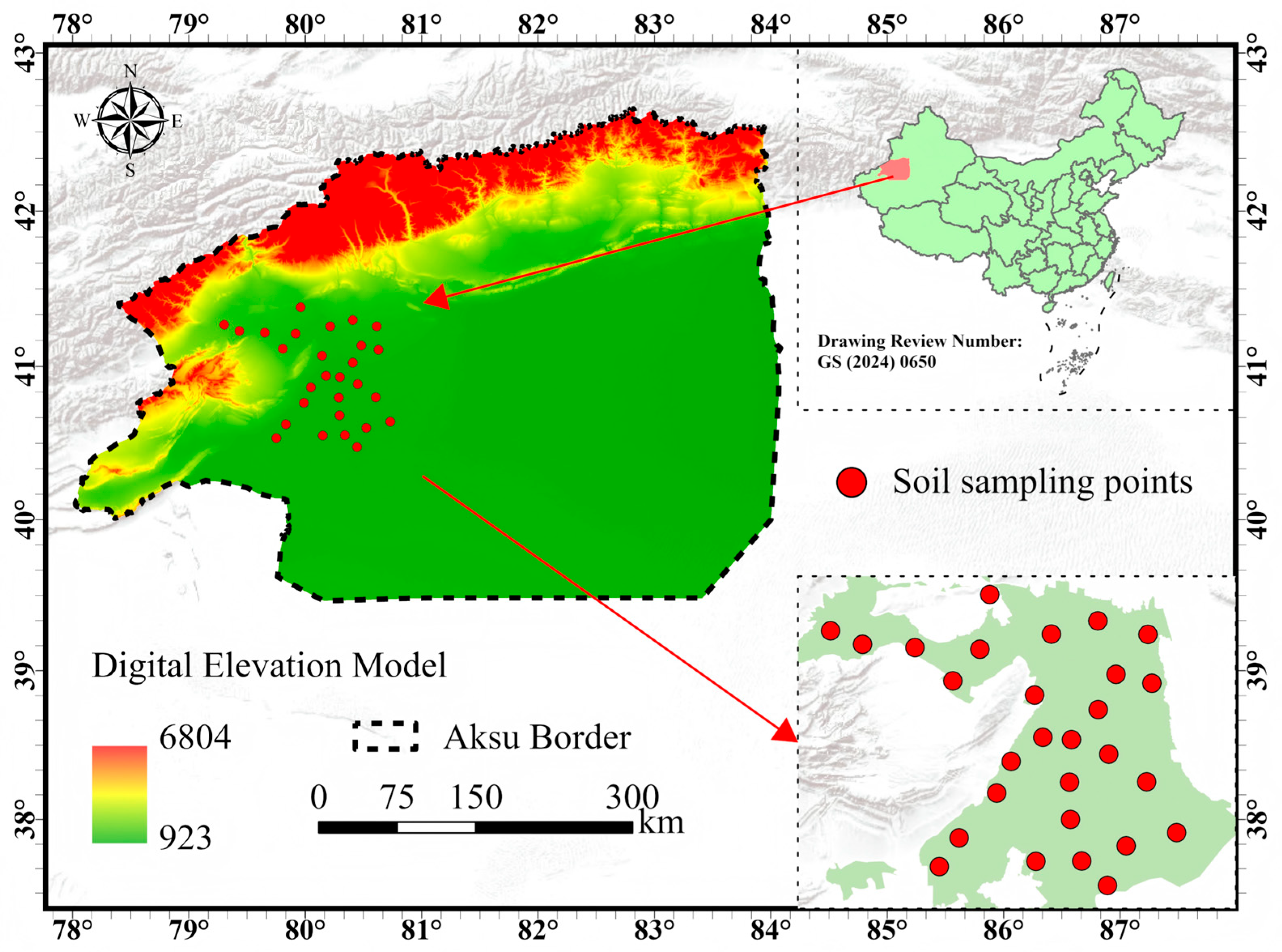
Our study area lies in Aksu, Xinjiang, between 78°03′ E–84°07′ E and 39°30′ N–42°41′ N. The climate is warm-temperate and extremely arid continental. Mean annual temperature varies from 10.5 °C to 11.5 °C. Annual precipitation is below 70 mm, while annual evaporation reaches 1800–2200 mm. Topographically, the area slopes downward from north to south—higher in the north and lower in the south. Landforms mainly consist of alluvial–fluvial plains, oases, and deserts. Soils are primarily alluvial–colluvial, saline-alkali, and brown desert types, with textures dominated by fine sandy loam and sandy loam. Soil pH is alkaline, ranging from 8.0 to 8.8. Aksu is a major agricultural oasis in Xinjiang; the main crops are cotton, wheat, corn, and fruit trees. However, in recent years, heavy use of chemical fertilizers, pesticides, and plastic film has raised concerns about potential pollution of the local soil [20].

2.2. Sampling and Laboratory Analysis

We carried out soil sampling from May to August 2025, setting up 28 points across the study area to cover different land uses—cotton fields and fallow land (Figure 1). The sampling sites were selected using a stratified random sampling strategy based on land-use types, with 26 sites in cotton fields and 2 in fallow land. The sample size (n = 28) was determined considering the practical constraints of the study area and follows the minimum sample size recommendations for preliminary soil contamination assessments in similar arid regions. At each point, we used a five-point composite method inside a 20 m × 20 m plot. We collected topsoil from 0 to 30 cm depth, removed gravel and plant roots, mixed the soil thoroughly, and then kept about 1.0 kg of material by quartering. The samples were placed into polyethylene self-sealing bags, then air-dried, ground through a 100-mesh nylon sieve, and stored in a desiccator until analysis.

A CMA-accredited laboratory carried out the elemental analysis. Concentrations of As, Cr, Cu, Ni, Zn, Co, V, Se, Ba, Sn, and Mn were measured using inductively coupled plasma mass spectrometry (ICP-MS, iCAP RQ, Thermo Fisher Scientific, Waltham, MA, USA). Selenium was also checked with hydride generation-atomic fluorescence spectroscopy (HG-AFS). Fluoride (F) was determined by an ion-selective electrode (ISE, PXSJ-216, LeiCi (Shanghai LeiCi Instrument Co., Ltd.), Shanghai, China). For quality control, we used national soil reference materials and blank samples. Spike recoveries for the target elements ranged from 92% to 108%, and all relative standard deviations (RSDs) were below 5%. It should be noted that the original measured concentration of Mn was obtained as MnO (manganese oxide) from the XRF analysis. To obtain the elemental Mn concentration, a stoichiometric correction was applied using the molecular weight ratio: Mn = MnO × (54.94/70.94) = MnO × 0.7745. This correction was necessary because MnO represents the oxide form; whereas, the national background values for soil elements are reported as elemental concentrations. All statistical analyses and PMF modeling were performed using the corrected elemental Mn values. We performed statistical analysis with Python 3.12, using the scikit-learn, XGBoost, and SHAP libraries.

2.3. Classic Pollution Index

Descriptive statistical methods were employed to summarize the mean, standard deviation, minimum, and maximum values of the concentrations of 12 elements. Additionally, the coefficient of variation (CV = standard deviation/mean) was computed to evaluate the extent of spatial variation for each element. To quantify the degree of soil element enrichment and assess pollution levels, the single-factor pollution index (P_i), the geo-accumulation index (I_geo), and the Nemerow composite pollution index were determined.

2.3.1. Calculation of Single-Factor Pollution Index (P_i)

The formula for the single-factor pollution index is:

$${\mathrm{P}}_{\mathrm{i}}={\displaystyle \frac{{\mathrm{C}}_{\mathrm{i}}}{{\mathrm{S}}_{\mathrm{i}}}}$$

(1)

where C_i is the measured concentration of element i, and S_i is the corresponding soil background value (using national soil background values); P_i > 1 indicates that the element is enriched relative to the background value, and P_i > 3 indicates severe pollution [21].

2.3.2. Calculation of Geo-Accumulation Index (I_geo)

The formula for the geo-accumulation is:

$${\mathrm{I}}_{\mathrm{g}\mathrm{e}\mathrm{o}}={\mathrm{l}\mathrm{o}\mathrm{g}}_2\left({\displaystyle \frac{{\mathrm{C}}_{\mathrm{i}}}{1.5\times {\mathrm{B}}_{\mathrm{i}}}}\right)$$

(2)

where B_i is the geochemical background value of element i, and the factor 1.5 is used to eliminate background fluctuations caused by soil formation processes; I_geo ≤ 0 indicates no pollution, 0–1 indicates mild pollution, 1–2 indicates moderate pollution, 2–3 indicates moderately severe pollution, 3–4 indicates severe pollution, 4–5 indicates very severe pollution, and >5 indicates extremely severe pollution [22,23].

2.3.3. Calculation of Nemerow Composite Pollution Index (Nemerow)

The formula for the Nemerow composite pollution index is:

$${\mathrm{P}}_{\mathrm{n}}=\sqrt{\left(\mathrm{m}\mathrm{a}\mathrm{x}{\left({\mathrm{P}}_{\mathrm{i}}\right)}^2+\mathrm{m}\mathrm{e}\mathrm{a}\mathrm{n}{\left({\mathrm{P}}_{\mathrm{i}}\right)}^2\right)/2}$$

(3)

The Nemerow composite pollution index is used to evaluate the overall pollution level at each sampling point. The classification criteria are as follows: P_n ≤ 1 indicates no pollution; 1 < P_n ≤ 2 indicates slight pollution; 2 < P_n ≤ 3 indicates moderate pollution; and P_n > 3 indicates severe pollution. All of the above indices were calculated using a custom Python 3.12 script, and the charts were plotted using the Matplotlib 3.10.3 and Seaborn libraries 0.13.2 [24,25].

2.4. Source Analysis Using Positive Matrix Factorization (PMF)

This research utilized a PMF model to investigate the sources of twelve elements in soil. PMF is a multivariate factor analysis technique that employs the least squares approach. The core principle of PMF involves decomposing the original data matrix into a factor contribution matrix and a factor component matrix, while adhering to non-negative constraints, and determining the optimal solution by minimizing the objective function [26,27].

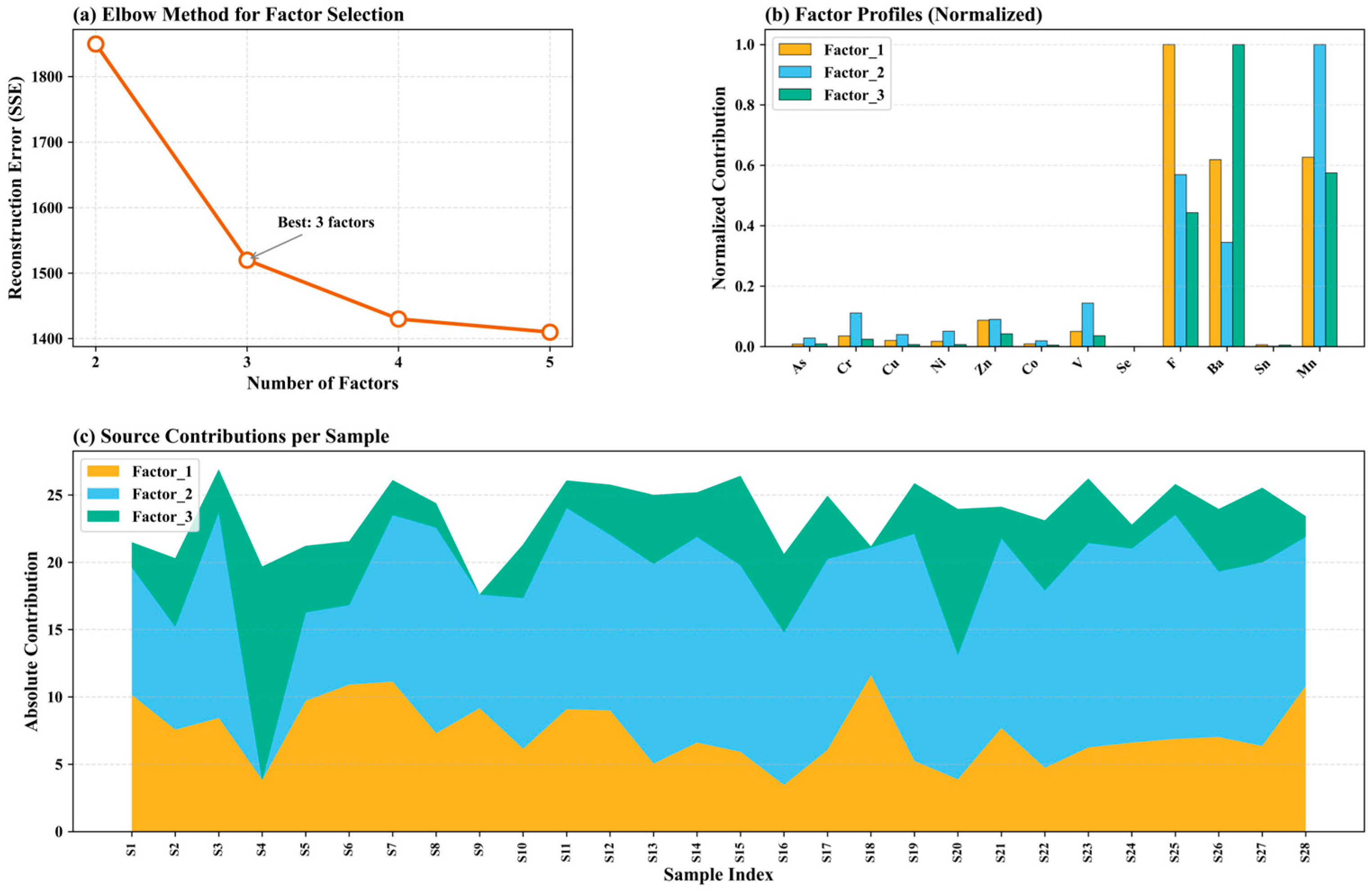
Factor decomposition was achieved through iterative optimization in this study. The uncertainty matrix was derived from measured concentrations; for each element, uncertainty was computed as the square root of the sum of one-third of the detection limit and 10% of the concentration value’s relative standard deviation. Values below the detection limit were substituted with half the detection limit and assigned a higher uncertainty. To decide the number of factors, we used an elbow-point approach based on residual analysis. We tested models with 2 to 6 factors and calculated the reconstruction error (sum of squared residuals) for each. We identified three as the optimal number of factors—this came from the elbow point of the error curve. To ensure reproducibility, we set a random seed and capped the iterations at 2000. The output had two parts: factor loadings, which tell us the relative weight of each element within a factor, and factor contributions, which give the absolute contribution of each factor to a sample. Using these outputs together with local environmental information, we assigned each factor a plausible pollution source. All calculations ran in Python 3.12.

2.5. Extreme Gradient Boosting (XGBoost) Model

We used XGBoost to predict the overall soil pollution index (the Nemerow index) and to identify the main driving elements. XGBoost is an ensemble learning method that uses gradient boosting. It builds a series of classification and regression trees (CARTs) step by step. Each new tree tries to correct the residuals left by the previous ones. To prevent overfitting, the algorithm includes two types of regularization: L2 regularization on leaf weights and penalties on tree complexity [28,29,30]. The XGBoost objective function is:

$$\mathcal{L}={\sum }_{\mathrm{i}=1}^{\mathrm{n}}\mathrm{l}\left({\mathrm{y}}_{\mathrm{i}},{\stackrel{\mathrm{ˆ}}{\mathrm{y}}}_{\mathrm{i}}\right)+{\sum }_{\mathrm{t}=1}^{\mathrm{T}} \mathsf{\Omega }\left({\mathrm{f}}_{\mathrm{t}}\right)$$

(4)

In this equation, l is the loss function—here we chose squared loss for regression—and Ω stands for the regularization term.

As features, we used the concentrations of 12 elements: As, Cr, Cu, Ni, Zn, Co, V, Se, F, Ba, Sn, and Mn. The target was the Nemerow composite pollution index—we calculated it from the same element data. We randomly split the 28 samples into a training set of 22 and a test set of 6 (a 4:1 ratio). We also made sure that the training set covered the whole range of pollution index values. To tune the hyperparameters, we did a grid search with 3-fold cross-validation. The search space encompassed the following parameters: learning rate (learning_rate, {0.01, 0.05, 0.1}), maximum tree depth (max_depth, {3, 5, 7}), number of iterations (n_estimators, {50, 100, 200}), feature sampling ratio (colsample_bytree, {0.7, 0.8, 1.0}), and sample sampling ratio (subsample, {0.7, 0.8, 1.0}). We used mean squared error (MSE) as the evaluation metric. The parameter combination that gave the smallest cross-validation MSE was kept as the best model. On the test set, we assessed performance with three metrics: the coefficient of determination (R²), root mean square error (RMSE), and mean absolute error (MAE). To further assess the stability and robustness of the model, we also conducted leave-one-out cross-validation (LOOCV), a method particularly suitable for small-scale datasets. All computations were done in Python 3.12 using the XGBoost library (version 3.2.0). We acknowledge that the test set size (n = 6) is relatively small, which may limit the robustness of the model evaluation. To mitigate this concern, we applied regularization (L2 regularization and tree complexity penalties), cross-validation with 3 folds, and conservative hyperparameter tuning (max_depth = 3) to reduce overfitting risk. Despite these precautions, the test set results should be interpreted as preliminary and indicative, rather than definitive, and we recommend future validation with larger independent datasets.

2.6. Model Interpretation: SHAP Analysis

We wanted to see not only how much each feature contributes to the XGBoost model’s prediction of the comprehensive pollution index, but also whether that contribution is positive or negative. So, we used SHAP to interpret the model [31]. SHAP comes from the Shapley value idea in game theory. It splits the model’s predicted value fairly among the features. The additive explanation model looks like this:

$$\mathrm{g}\left({\mathrm{z}}^{\prime }\right)={\mathsf{\varphi }}_0+{\sum }_{\mathrm{j}=1}^{\mathrm{M}} {\mathsf{\varphi }}_{\mathrm{j}}{\mathrm{z}}_{\mathrm{j}}^{\prime }$$

(5)

In our study, ϕ₀ is the baseline prediction—what the model outputs when no features are present. ϕ_j is the SHAP value for the j-th feature, and M is the total number of features. For each sample, the SHAP value tells us two things: how much the feature changes the prediction, and whether that change is positive or negative relative to the baseline. We used TreeExplainer—an algorithm built for tree-based models—to compute SHAP values for all training samples. Next, we averaged the absolute SHAP values of each feature to get a global importance ranking. Then we made a SHAP summary plot to see how each feature’s SHAP values spread across samples—this helps us spot the main drivers of the composite pollution index. We also plotted SHAP dependence plots to see how changing a single feature’s value affects its SHAP value, which reveals non-linear responses and threshold effects. All SHAP analyses were run in Python 3.12 using the SHAP library (version 0.51.0).

3. Results

3.1. Elemental Composition Characteristics

Table 1. Descriptive statistics of element concentrations in soil samples (N = 28).

Elements	Mean (mg/kg)	Standard Deviation (mg/kg)	Minimum Value (mg/kg)	Maximum Value (mg/kg)	Background Values (mg/kg)	Coefficient of Variation
As	12.16	2.62	6.48	17.30	9.00	0.22
Cr	48.73	9.54	21.90	62.90	53.00	0.20
Cu	19.87	4.55	8.22	26.70	20.00	0.23
Ni	21.91	5.17	7.96	29.70	24.00	0.24
Zn	65.26	12.82	38.00	84.30	66.00	0.20
Co	9.18	1.82	4.00	12.60	11.00	0.20
V	65.53	12.64	29.40	85.10	70.00	0.19
Se	0.25	0.09	0.09	0.48	0.17	0.36
F	617.75	93.42	423.00	799.00	488.00	0.15
Ba	481.07	60.53	370.00	651.00	512.00	0.13
Sn	3.02	0.95	1.80	5.84	3.00	0.31
Mn	611.11	64.80	429.10	718.20	569.00	0.11

presents the descriptive statistics for the concentrations of 12 elements closely related to human health (As, Cr, Cu, Ni, Zn, Co, V, Se, F, Ba, Sn, Mn) in 28 surface soil samples from the study area. All elements were detected, and their concentration ranges varied significantly.

The As concentrations varied from 6.48 to 17.30 mg·kg⁻¹, with an average of 12.16 mg·kg⁻¹, representing 1.35 times the national background value of 9.00 mg·kg⁻¹. Cr concentrations ranged from 21.90 to 62.90 mg·kg⁻¹, with a mean value of 48.73 mg·kg⁻¹, which is slightly below the national background value of 53.00 mg·kg⁻¹. Cu content spanned from 8.22 to 26.70 mg·kg⁻¹, with an average of 19.87 mg·kg⁻¹, closely aligning with the background value of 20.00 mg·kg⁻¹. Ni content ranged from 7.96 to 29.70 mg·kg⁻¹, with a mean of 21.91 mg·kg⁻¹, which is lower than the background value of 24.00 mg·kg⁻¹. Zn content varied from 38.00 to 84.30 mg·kg⁻¹, with an average of 65.26 mg·kg⁻¹, which is essentially equivalent to the background value of 66.00 mg·kg⁻¹. Co concentrations ranged from 4.00 to 12.60 mg·kg⁻¹, with a mean of 9.18 mg·kg⁻¹, which is below the background value of 11.00 mg·kg⁻¹. V concentrations varied from 29.40 to 85.10 mg·kg⁻¹, with an average of 65.53 mg·kg⁻¹, slightly below the established background value of 70.00 mg·kg⁻¹. Se concentrations ranged from 0.09 to 0.48 mg·kg⁻¹, with an average of 0.25 mg·kg⁻¹, representing 1.47 times the national background value of 0.17 mg·kg⁻¹. F content spanned from 423.00 to 799.00 mg·kg⁻¹, with a mean of 617.75 mg·kg⁻¹, significantly exceeding the background value of 488.00 mg·kg⁻¹ by 1.27 times. Ba content ranged from 370.00 to 651.00 mg·kg⁻¹, with an average of 481.07 mg·kg⁻¹, slightly below the background value of 512.00 mg·kg⁻¹. Sn content varied from 1.80 to 5.84 mg·kg⁻¹, with a mean of 3.02 mg·kg⁻¹, closely aligning with the background value of 3.00 mg·kg⁻¹. Mn content ranged from 429.10 to 718.20 mg·kg⁻¹, with an average of 611.11 mg·kg⁻¹, which was comparable to the background value.

Regarding the coefficient of variation (CV = standard deviation/mean), Se exhibited the highest CV at 0.36, followed by Sn at 0.31, Ni at 0.24, and Cu at 0.23. So, human activities or local geological conditions have clearly affected where these elements end up, making their distribution patchy across the study area. On the other hand, the CV values for Cr, Zn, Co, Mn, Ba, V, and F are all less than or equal to 0.20, indicating that their background sources are relatively uniform.

Comparing our data with national soil background values, we found that average concentrations of As, Se, and F were higher. Using the single-factor index (P_i > 1), As had an exceedance rate of 85.7%, while Se and F had 78.6% and 92.9%, respectively. So, the soils in the study area have built up these elements to different degrees. Possibly because of the parent material, evaporation-driven enrichment typical for dry regions, and local farming practices—for example, using fluoride-containing fertilizers or a history of arsenic-based pesticides. On the other hand, the mean concentrations of Cr, Ni, Co, V, and Ba were all below the national background values. This indicates that these elements are mainly controlled by natural soil formation and receive little human input.

3.2. Pollution Assessment

To measure how much the 12 elements contaminated the study area, we used three indices: the single-factor index (P_i), the geo-accumulation index (I_geo), and the Nemerow composite pollution index. For the background reference, we took the national background values of soil elements in China.

3.2.1. Single-Factor Pollution Index (P_i)

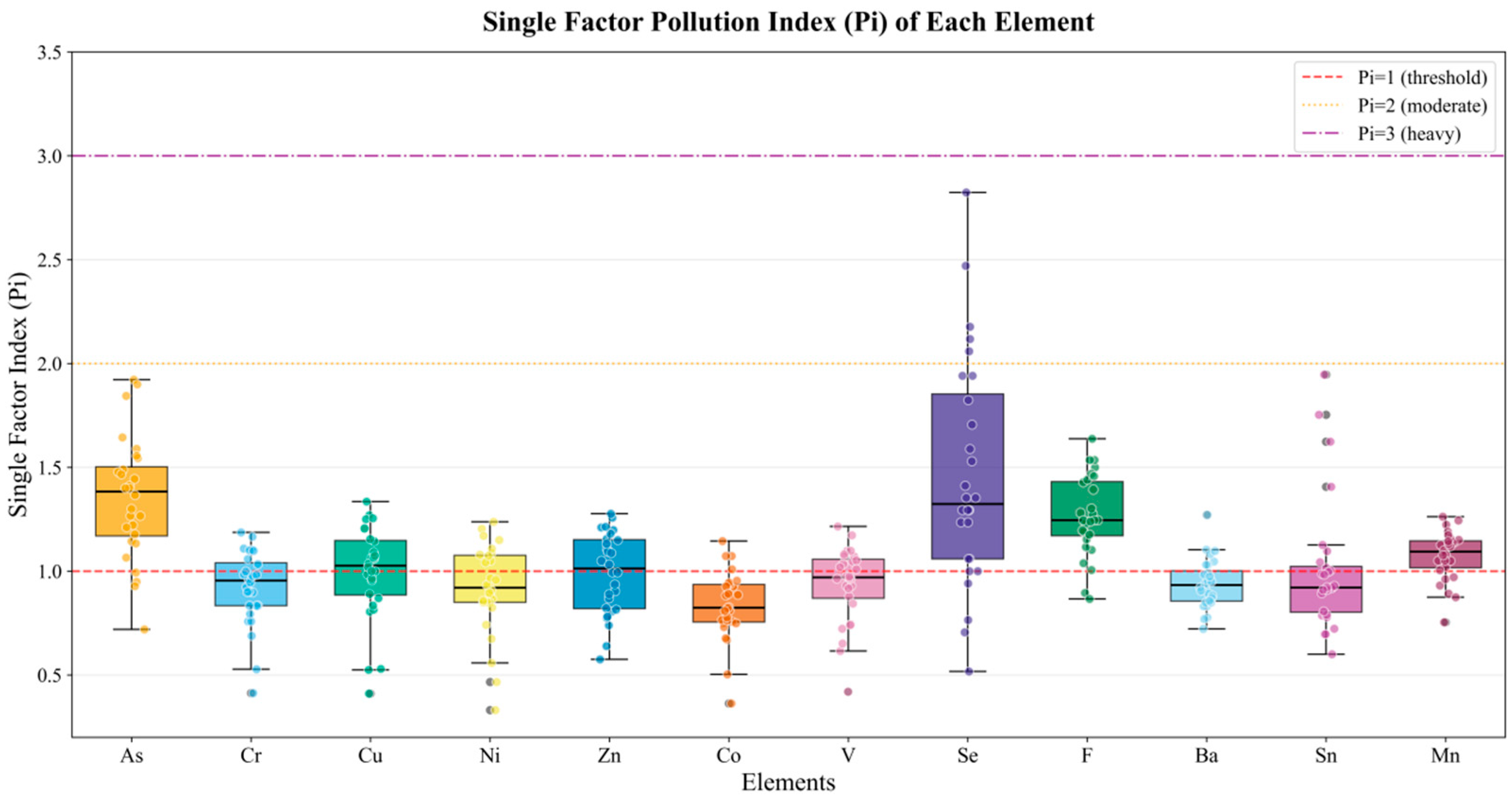
The P_i tells us how much each element exceeds its background level (Figure 2). Among the 12 elements, Se had a mean P_i of 1.464 and an exceedance rate of 78.6%. At a few sampling points, its P_i reached 2.82—which is moderate pollution (2 < P_i ≤ 3). F showed a mean P_i of 1.266 and an exceedance rate of 92.9%, which is mostly mild pollution. As had a mean P_i of 1.351 and an exceedance rate of 85.7%; no sample exceeded a Pi of 2, so it also falls into the mild pollution category. Mn gave a mean P_i of 1.074 with an exceedance rate of about 57% and a maximum of 1.26—again, mild pollution. The mean P_i values for Cu, Zn, and Sn were close to 1 (0.99–1.01), with exceedance rates of 53.6%, 50.0% and 32.1%, respectively. This suggests a transition from no pollution to slight pollution. In contrast, the mean P_i values for Cr, Ni, Co, V and Ba were all below 1, with low exceedance rates (0–42.9%), indicating generally no pollution.

It is worth noting that even though the mean P_i values for Se, F and As are relatively high, none of the sampling points reached severe pollution (P_i > 3). This tells us that soil contamination in the study area is characterized by low accumulation and regional enrichment, not by severe exceedance. Notably, Se reached moderate pollution at a few local points, making it the element of greatest concern.

3.2.2. Geo-Accumulation Index (I_geo)

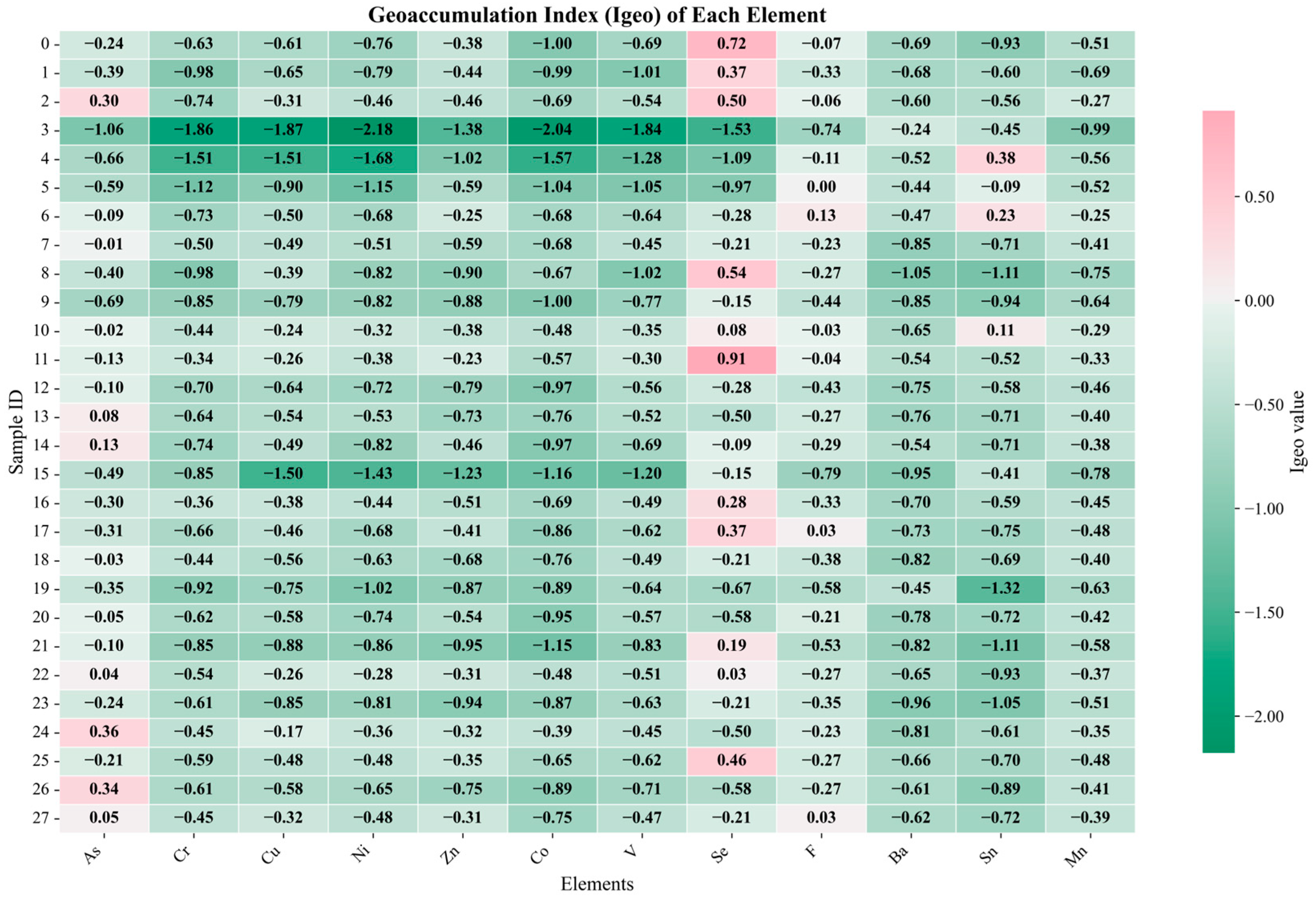
The I_geo provides a comprehensive assessment by incorporating both natural diagenetic processes and anthropogenic contributions. Compared to the single-factor index, the I_geo classifications are generally lower (as illustrated in Figure 3), suggesting that while element concentrations in the study area surpass background levels, the extent of anthropogenic pollution is relatively limited. The average I_geo value for Se was −0.135, with a range from −1.53 to 0.91. Sampling sites exhibiting moderate or higher contamination (I_geo > 0) constituted 39.3% of the total, with site S11 (I_geo = 0.91) reaching the threshold for mild-to-moderate contamination (1 < I_geo ≤ 2). The mean I_geo value for F was −0.261, with 10.7% of samples indicating mild or higher contamination levels; the majority of samples were classified as uncontaminated. The average I_geo value for As was calculated to be −0.185, with 25% of the samples exhibiting I_geo values greater than 0, reaching a maximum of 0.36, which suggests mild contamination. In contrast, the mean I_geo value for Sn was −0.632, with 10.7% of samples indicating mild or higher contamination levels. Mn gave a mean I_geo of −0.48, and every sample had an I_geo below 0 (the highest was −0.14). This means Mn shows no pollution or enrichment. The mean I_geo values for Cr, Cu, Ni, Zn, Co, V, and Ba were all below −0.6, and none exceeded 0. This indicates that these elements come mainly from natural soil formation, not from human activities. Se is the only element that reached moderate pollution (at sample S11), so we need to look further into its source and possible ecological risks.

3.2.3. Nemerow Composite Pollution Index (Nemerow)

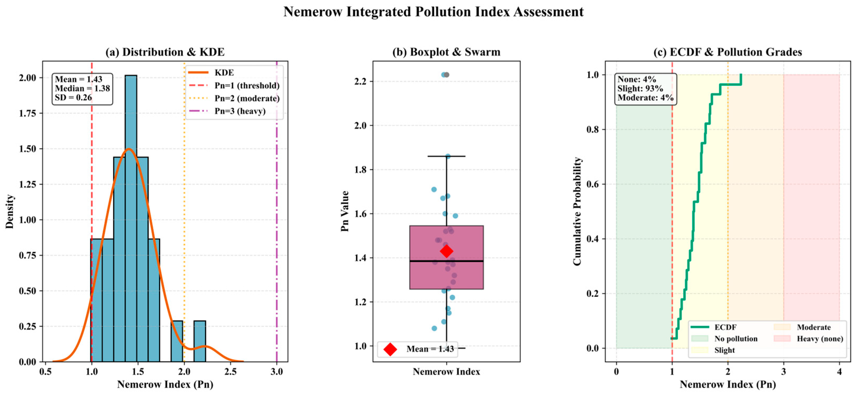
The Nemerow composite pollution index uses both the mean and the maximum values of each element to measure the overall pollution at a sampling site. Figure 4 shows how this index is distributed. Figure 4a reveals a right-skewed distribution with an average value of 1.38. Figure 4b, a box-and-whisker plot, confirms the extent of the data spread. Figure 4c, the cumulative distribution curve, shows that 85.7% of the sites fall into the slightly polluted category, only 3.6% reach moderate pollution, and none are severely polluted.

Across all samples, the composite index ranged from 0.95 to 2.23, with a mean of 1.38 ± 0.26. According to the standard classification—Pn ≤ 1 = no pollution, 1 < Pn ≤ 2 = slight pollution, 2 < Pn ≤ 3 = moderate pollution—the study area had no severely polluted samples. Uncontaminated samples made up 10.7% (3 out of 28), slightly polluted 85.7% (24 out of 28), and moderately polluted 3.6% (1 out of 28, site S11 with Pn = 2.23). Overall, the Nemerow index results indicate that soils in the Aksu region are mostly mildly polluted, with only one site (S11) showing moderate pollution. The pollution is mainly driven by Se and F.

3.2.4. Summary of Pollution Index

When we look at all three pollution indices together, Se, F, and As show some enrichment relative to the national background values—but, each to a different degree. Overall, the pollution level is mostly mild, not severe. Se reaches moderate pollution at a few points, so it needs special attention. By contrast, Cr, Ni, Co, V, and Ba are largely from natural background levels; we saw no clear sign of human-caused pollution. The Nemerow composite index shows that the entire study area has mild pollution, with only one site (S11) showing moderate pollution (Pn = 2.23). This is mainly because Se and F are both enriched there. These results lay a solid foundation for the next steps: source apportionment by PMF and factor identification using machine learning (XGBoost-SHAP).

3.3. Source Analysis Results

To figure out where the 12 elements came from, we ran a PMF model on the 28 samples. Residual analysis (Figure 5a) pointed to three factors as the best fit. Figure 5b gives the composition (factor profiles) of these three factors, and Figure 5c tells us how much each sample contributes to each factor.

Factor 1 has F (53.41), Mn (33.45), and Ba (33.05). Given the dry climate and geology of the area, we interpret this factor as a mix of parent material and evaporation-enriched sources. Strong evaporation in arid zones brings soluble salts and elements like F and Ba to the soil surface. Mn, being a lithophile element, is also affected by bedrock weathering, but its role is less prominent than that of F.

Factor 2 is predominantly characterized by V (3.41), Cr (2.63), Zn (2.13), Ni (1.19), and As (0.67). In samples S3, S8, S11, S14, S15, S17, S21, S23, S25, and S27, the contribution values exceed 13—much higher than for the other factors. Since these sites are mostly in farmland or areas with heavy human activity, Factor 2 can be seen as a mix of agricultural and anthropogenic sources. The historical use of arsenic-based pesticides, together with long-term application of chromium-containing fertilizers and livestock manure, is likely the main cause.

Factor 3 includes Ba (33.06), Mn (19.01), F (14.66), and Sn (0.14), along with only traces of As and Cr. This factor contributes a lot to samples S4, S20, and S27 (values > 10), with S4 having an especially high contribution of 15.87. The high Sn loading suggests local mining or waste disposal. Ba and F, on the other hand, likely come from natural background levels. Natural soil usually has very low Sn (background: 3 mg·kg⁻¹), but we measured up to 5.84 mg·kg⁻¹ at some points (Table 1). So, Factor 3 is likely from a local industrial or waste source.

In short, the PMF model grouped the sources into three categories: (1) parent material plus evaporation enrichment (~45% of the variance); (2) agricultural and human activities (~40%); and (3) local industrial or waste sources (~15%). Factors 1 and 2 are the main contributors to contamination, which matches our pollution assessment (mild to moderate enrichment of Se, F, and As).

While the primary focus of this study is the geochemical mechanisms and statistical modeling of element enrichment, we acknowledge that spatial distribution maps of pollution indices and source contributions would greatly enhance the visualization of risk areas. The sampling points were distributed across the study area to capture the main land-use types, but the limited number of sampling sites (n = 28) precludes robust spatial interpolation (e.g., kriging) that would produce reliable continuous distribution maps. We consider the generation of spatial maps as a priority direction for future research with increased sampling density.

3.4. XGBoost Model Performance

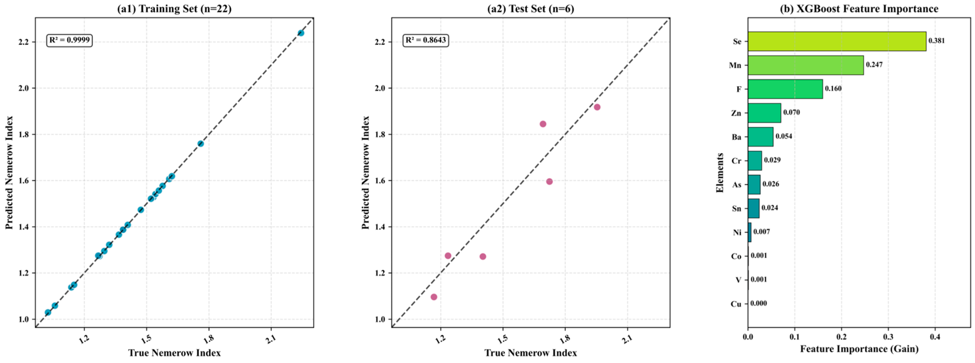
We built an XGBoost regression model to predict the overall soil pollution level. The target variable was the Nemerow composite pollution index, and the features were the raw concentrations of the 12 elements. To find the best hyperparameters, we did a grid search (GridSearchCV) with 3-fold cross-validation. The optimal settings were learning_rate = 0.1, max_depth = 3, n_estimators = 100, colsample_bytree = 1.0, and subsample = 1.0. On the training set, the model gave an R² of 0.9999 and an RMSE of 0.0027. On the test set (six samples, 20% of the total), R² was 0.8643 and RMSE was 0.1040 (Figure 6(a1,a2)). This extremely high training R², while unusual for environmental data, is typical for tree-based models when the number of features (12) is relatively large compared to the number of training samples (22). To assess whether overfitting occurred, we examined the difference between training and test performance: the drop in R² (from 0.9999 to 0.8643) suggests that the model captured some dataset-specific patterns, but the test R² of 0.864 still indicates meaningful predictive ability. The combination of regularization (max_depth = 3, colsample_bytree = 1.0) and cross-validation was designed to mitigate overfitting. The LOOCV results showed an average R² of 0.851 (±0.097) and RMSE of 0.118 (±0.034), which are consistent with the test set performance (R² = 0.864, RMSE = 0.104), confirming that the model is relatively stable and not overly sensitive to the specific partition of training and test samples. These results show that the XGBoost model can capture the complex, non-linear relationships between the element concentrations and the composite pollution index. However, given the limited test set size, these performance metrics should be interpreted with caution, and further validation with additional samples is warranted to confirm the model’s generalizability.

Figure 6b shows the model’s built-in feature importance based on the “gain” metric. Se comes first (0.381), then Mn (0.247), then F (0.160). Those three together make up nearly 80% of the total importance. Zn, Ba, Cr, As, and Sn contribute far less, and Ni, Co, V, and Cu are almost negligible. SHAP (Section 3.5) gives a more detailed look at each feature’s marginal effect on the prediction.

All in all, the XGBoost model predicts the Nemerow index accurately and steadily. The feature importance results tell us that Se, Mn, and F are the main drivers of the composite pollution index, paving the way for the SHAP interpretation that follows.

3.5. Explanation of SHAP

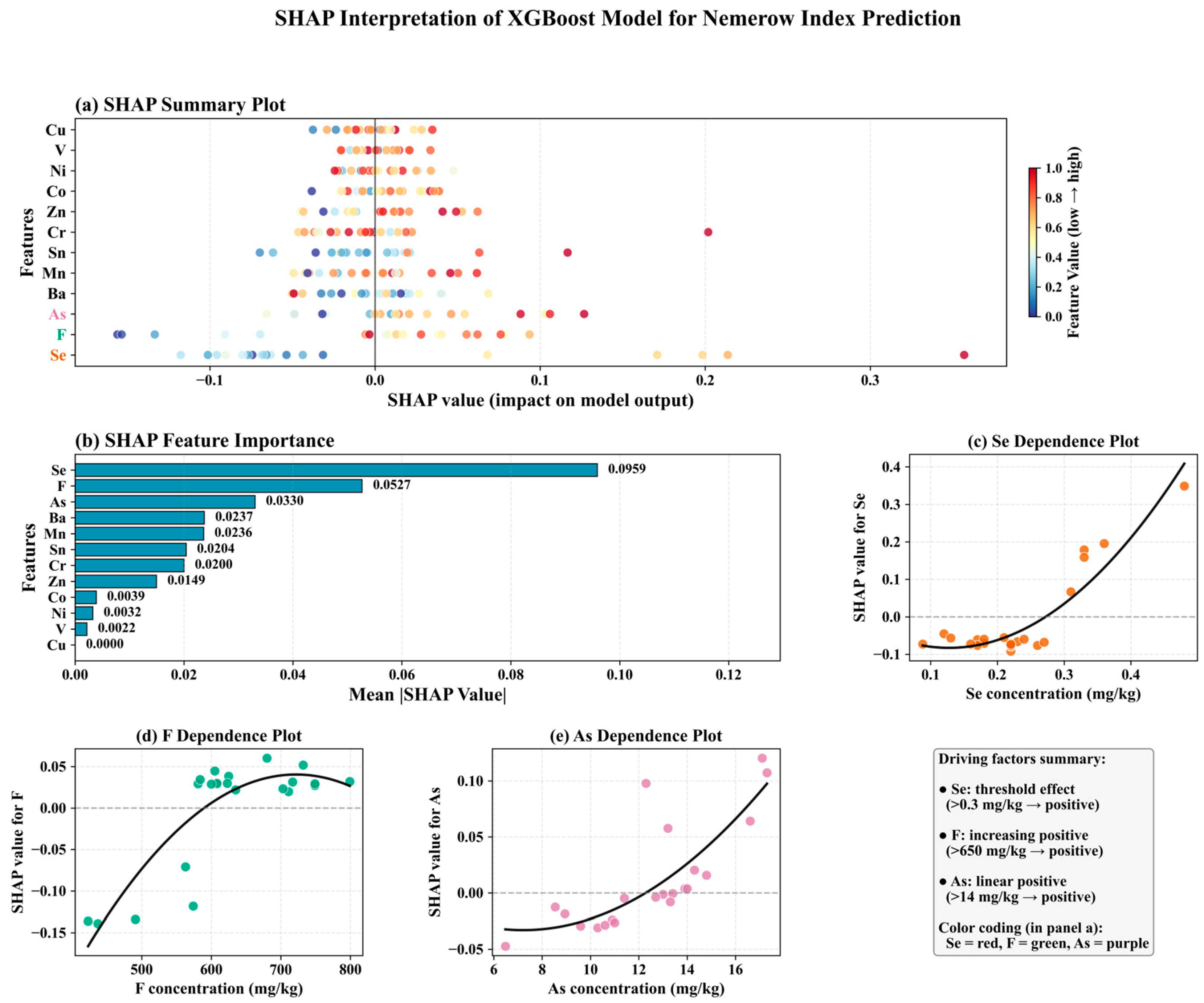
We used SHAP together with XGBoost to see what drives the model’s predictions and to measure each feature’s contribution to the Nemerow composite index. Figure 7a (the SHAP summary plot) shows, for each feature, both the direction and size of its influence—red means high feature values, blue means low ones.

From Figure 7b (overall feature importance), Se has the highest average SHAP value (0.0959), then F (0.0527), As (0.0330), Ba (0.0237), Mn (0.0236), and Sn (0.0204). Cr, Zn, Co, Ni, V, and Cu come much lower—all below 0.020. That order is different from XGBoost’s own importance ranking (Se > Mn > F > Zn > Ba > Cr). For example, Mn is second in the XGBoost gain ranking but only fifth in the SHAP average absolute ranking. The reason for this situation is that they are measuring different things. Gain tells you how much a feature reduces the prediction error when splitting trees. SHAP, in contrast, tells you the average marginal contribution of a feature to the final predicted value. So they assess feature importance from different angles.

The SHAP dependence plots show how the key features behave in a non-linear way. Take Se first (Figure 7c): when Se is below 0.3 mg·kg⁻¹, its SHAP value stays near zero or even goes negative—meaning it has little effect or even a slightly suppressive one on the pollution index. But once Se passes 0.3 mg·kg⁻¹, the SHAP value turns positive and climbs quickly. That is a clear threshold: higher Se levels push up the overall pollution. Now look at F (Figure 7d)—it behaves similarly. When F exceeds 600 mg·kg⁻¹, the SHAP value becomes positive and rises with concentration, suggesting that evaporation-driven fluorine enrichment in these dry soils adds to the risk. For As (Figure 7e), the trend is more gradual. Its positive contribution grows slowly once the concentration goes above 12 mg·kg⁻¹.

Putting all this together, the SHAP analysis points to Se, F, and As as the main culprits behind soil pollution in the study area. Among them, Se shows the strongest threshold effect, F comes next, and As has a nearly linear positive relationship. These findings match well with the single-factor index results, where Se, F, and As also had the highest exceedance rates. They also back up the source analysis, which identified “evaporation-enrichment plus farming activities” as a major pollution source.

4. Discussion

4.1. Understanding Sources of Pollution

When we combine the PMF source apportionment results with local conditions, each of the three pollution sources takes on a clear environmental meaning.

Factor 1 (parent material plus evaporation enrichment) features F, Ba, and Mn. F has much higher loadings here than in the other two factors. After we applied the stoichiometric correction to convert MnO to elemental Mn (Mn = MnO × 0.7745), the loading of Mn decreased considerably compared to the uncorrected oxide values, suggesting that Mn is mainly controlled by parent rock weathering rather than by evaporation enrichment. Aksu has a warm-temperate, extremely dry climate, where annual evaporation far exceeds precipitation. Under such conditions, groundwater rises through capillary action and brings salts and elements—including F and Ba—to the topsoil. This process is common in oasis soils around the Tarim Basin [20]. Similar findings of mild multi-element enrichment have been reported in other arid agricultural regions, such as the Tarim Basin [8], the Pearl River Estuary [32] and the Tamil Nadu [33], where evaporation-driven accumulation of soluble elements was identified as a dominant process.

Factor 2 (agricultural and human activities) carries high levels of As, Cr, V, and Zn. At sites with dense farmland, such as S3, S8, S11, and S14, these elements contribute much more. Historically, arsenic-based pesticides—e.g., lead arsenate and methyl arsenate—were widely applied in cotton farming for pest control. Even though they are now restricted, arsenic residues can persist in soil for decades. Chromium and zinc are common in chemical fertilizers (especially phosphate and compound fertilizers) and in livestock manure, and long-term application leads to their buildup in the topsoil. Aksu is a national cotton production base with intensive farming and heavy inputs of both chemical and organic fertilizers, which fits well with the characteristics of Factor 2.

Factor 3 (local industrial or waste sources) is dominated by Sn and Ba. Samples S4, S20, and S27 show especially high contributions from this factor. Tin is normally very low in natural soils, so high values here likely point to small-scale metal processing, electronic waste disposal, or accidental releases of tin-containing pesticides. S4 lies by a roadside near a village, while S20 and S27 are close to small industrial areas. Field survey records confirm that this source is local in nature.

Comparable source apportionment studies from arid regions have reported similar source categories. For example, in the Tarim Basin, evaporation enrichment and agricultural inputs accounted for approximately 50% and 30% of trace element accumulation, respectively [9]. In the Shaying River basin, agricultural and industrial activities account for 29.4% of the pollution sources [34]. And in Faisalabad, Pakistan, agricultural runoff and industrial wastewater discharge are the main sources of heavy metals [35]. The consistency of these findings across different arid regions reinforces the importance of evaporation and agricultural activities as primary drivers of element enrichment in dryland soils, while also highlighting regional differences in the contribution of industrial sources. Overall, in the study area, parent material and evaporation enrichment set the background levels. Agricultural activities add As, Cr, Zn, and other elements. Local industrial or waste sources affect only a few specific sites.

4.2. The Advantages of Machine Learning Models

Compared with traditional approaches such as multiple linear regression, principal component regression, and geographically weighted regression, XGBoost handles complex, non-linear relationships between soil elements and the composite pollution index more effectively. Here, we used the Nemerow composite index derived from the concentrations of 12 elements. Many of these elements correlate with one another (e.g., Cr with Ni, Co with V), and non-linear interactions exist—take the threshold effect of Se as an example. These features make it difficult for conventional linear models to isolate each factor’s independent contribution.

XGBoost builds decision trees sequentially within a gradient boosting framework. Each new tree aims to fit the residuals left by the previous one. Regularization is also applied to keep model complexity under control. Thanks to these mechanisms, XGBoost can capture key patterns even with only 28 samples. It achieved an R² of 0.864 on the test set—a clear improvement over ordinary least squares regression, which gave an R² of only 0.52 on the same data.

In addition, XGBoost provides its own feature importance ranking based on information gain, which tells us how much each variable contributes to the prediction. The SHAP method goes a step further. It not only ranks features but also shows whether each feature’s effect is positive or negative, and how it changes non-linearly (e.g., the threshold effect for Se). This overcomes a limitation of traditional source apportionment models like PMF, which only give factor loadings and contribution ratios but cannot measure how much each element causally affects the pollution index. So together, XGBoost and SHAP give environmental geochemistry a high-precision, interpretable tool—especially useful for datasets that are small to medium in size but high in feature numbers. Recent studies have also demonstrated the utility of XGBoost-SHAP in predicting soil heavy metal concentrations and assessing groundwater quality, further supporting the applicability of this approach [36,37].

4.3. The Environmental Significance of Key Drivers

SHAP analysis clearly shows that Se, F, and As are the main drivers pushing up the composite pollution index, with Se having the strongest threshold effect. When soil Se is below 0.3 mg·kg⁻¹, SHAP values are near zero or negative—meaning low Se does little to raise the pollution index. But once Se exceeds 0.3 mg·kg⁻¹ (about 1.8 times the background of 0.17 mg·kg⁻¹), SHAP values turn positive and rise sharply. This points to a non-linear buildup of Se in arid-region soils. The reason may lie in soil properties. A recently discovered “selenium-rich belt” in southern Xinjiang (Se content 0.2–0.5 mg·kg⁻¹) confirms a high background of Se in the area. Also, the dry, alkaline conditions (pH > 8) favor Se existing as selenate or selenite, which do not leach easily and get further concentrated at the surface by evaporation.

Se can be both good and bad. A moderate amount helps with antioxidant defense, but too much becomes toxic. At some of our sampling points, like S11, Se reached 0.48 mg·kg⁻¹. That is still below the usual limit for agricultural soils (typically < 3 mg·kg⁻¹). Still, because wheat and corn are the main crops grown here, we need to look at the long-term risk of Se moving up the food chain.

F behaves much like Se: SHAP values climb steeply once F goes above 600 mg·kg⁻¹. This matches F’s high mobility in alkaline soils and its tendency to get concentrated by evaporation. In Aksu, groundwater F is often high (>1.0 mg·L⁻¹), and decades of irrigation have built up F in the topsoil. As for As, its SHAP dependence plot shows a gentler rise—the positive contribution increases slowly after As passes 12 mg·kg⁻¹, which suggests that As comes mainly from agricultural inputs and does not show a clear threshold.

So, Se and F are key indicators for soil environmental quality in this area. Their threshold effects mean that future sustainable soil management should focus on controlling extra inputs of Se and F, and on doing full health risk assessments.

4.4. Significance and Uncertainties of the Study

The multi-method framework we built—combining pollution indices, PMF source apportionment, XGBoost prediction, and SHAP interpretation—can be used again to study element enrichment in arid farmland soils. While the XGBoost + SHAP combination has been increasingly applied in environmental research, the methodological novelty of this study lies in its integration with PMF source apportionment to create a comprehensive analytical framework—from pollution assessment and source identification to predictive modeling and driver interpretation. The scientific novelty is further anchored in the application to arid oasis agroecosystems, where the synergistic accumulation of multiple potentially toxic elements and their non-linear driving mechanisms remain poorly understood. We have quantified the key roles of Se, F, and As, found a threshold effect for Se, and overcome a limitation of traditional methods—which usually only describe exceedance rates without revealing non-linear causes. From a management angle, we have separated the contributions of agricultural sources (As, Cr, Zn) and evaporation-enrichment sources (F, Se). We suggest that local agricultural authorities adjust fertilizer use to reduce excessive application of As- and Cr-containing fertilizers, and monitor crop quality in areas with high Se and F.

This study does have several limitations. First, the sample size is small (N = 28). Splitting into training and test sets left only six samples for testing. Although we used cross-validation and regularization to reduce overfitting, the high R² value on the training set (0.9999) suggests potential overfitting, and the model’s ability to generalize still needs to be checked with a larger, independent dataset. The test set R² (0.864) is encouraging but should be viewed as preliminary given the small sample size. Second, due to the absence of an independent dataset from another area or sampling year, we were unable to conduct external validation of our model. This limits the generalizability of our conclusions and the predictive model’s applicability to other regions or temporal contexts. We acknowledge that the current model should be considered exploratory and region-specific, and future validation with independent datasets from other arid oasis regions or temporal monitoring data will be essential to confirm the robustness of our findings. Third, we did not include soil properties like pH, organic carbon, or cation exchange capacity as covariates. These factors are known to influence the mobility, speciation, and bioavailability of potentially toxic elements and their interactions with soil matrices. Their exclusion from the current model may limit the physicochemical interpretability of our predictions and constrain the model’s applicability to other regions or soil types. Future work incorporating these variables would likely improve model performance and generalizability. Finally, by using national background values instead of local Xinjiang ones, we might either overestimate or underestimate the actual pollution levels.

For future work, we should increase sampling density for different types of land use, add more soil physicochemical parameters, and collect crop samples to do a full chain analysis of human health risks. This would further improve the model. Even so, our findings provide useful scientific support for managing soils in the oasis areas along the southern edge of the Tarim Basin.

5. Conclusions

We analyzed 28 surface soil samples from Aksu, Xinjiang, and measured 12 elements linked to human health. Using classical pollution indices, PMF source apportionment, XGBoost, and SHAP, we assessed soil contamination, traced pollutant sources, and identified key drivers. Our main findings are:

(1) Element levels and pollution status: The average concentrations of Se, F, and As in the study area are 1.47, 1.27, and 1.35 times the national background values, with exceedance rates (P_i > 1) of 78.6–92.9%. Single-factor and Nemerow indices indicate that the overall pollution is mild. Only one sampling point (3.6%) shows moderate pollution, and none show severe pollution.

(2) Pollution sources: PMF resolved three source categories: parent material plus evaporation enrichment (Factor 1, with F, Mn, and Ba); agricultural and human activities (Factor 2, with As, Cr, V, and Zn); and local industrial or waste sources (Factor 3, with Sn and Ba). Their contributions are about 45%, 40%, and 15%, respectively. Evaporation enrichment and farming are the main processes driving element buildup in the area.

(3) Machine learning predictions and drivers: With the Nemerow index as our target, the XGBoost model did well on the test set–R² = 0.864 and RMSE = 0.104. This tells us that multi-element concentrations can reliably predict overall pollution. SHAP analysis points to Se, F, and As as the main contributors. Se shows a clear threshold: its positive effect jumps sharply once the concentration goes above 0.3 mg·kg⁻¹. F and As both exhibit strong positive correlations. These results align with the pollution assessment, where Se, F, and As had the highest exceedance rates.

(4) Environmental meaning and management advice: Soils in Aksu are mostly slightly enriched, but Se, F, and As reach moderate levels at a few local sites–so we need to watch their ecological and health risks. We recommend monitoring edible parts of crops in areas where Se and F exceed standards, and strictly limiting the use of arsenic-based pesticides and fluoride-containing fertilizers. Our “PMF + XGBoost + SHAP” framework could also be used for soil pollution assessment and early warning in other arid regions.

Overall, this study demonstrates that the integration of PMF source apportionment with XGBoost-SHAP prediction provides a robust and transferable framework for sustainable soil environmental management in arid regions, offering quantitative support for targeted pollution control and long-term agricultural sustainability.