Carbon-Neutrality Gap in Resource-Based Cities: STIRPAT Simulation and Cross-Validation of Carbon-Sink Models

Abstract

Coal-dominated resource-based cities face a structurally embedded carbon-neutrality gap, shaped by the simultaneous pressures of industrial carbon lock-in and ecological fragility. China’s dual-carbon targets impose severe transition pressure on such regions, where carbon-intensive industries, strong path dependence, and limited decarbonization flexibility compound the challenge. Forest carbon sinks offer a cost-effective approach for offsetting residual emissions. However, water scarcity and restricted land-carrying capacity impose hard ecological ceilings on sink expansion in semi-arid areas such as the Loess Plateau. Existing studies have largely focused on national or provincial scales, with few addressing the coupled dynamics of industrial emissions and water-limited sink capacity at the county level. This study examines Shenmu, China’s largest coal-producing county-level city and a national energy-chemical industrial base. Using time-series data spanning 2010–2025, we project multi-scenario carbon emissions via an extended STIRPAT model with ridge regression, estimate forest carbon sink potential through a growing-stock (GS) gradient model cross-validated against GM(1,1), and systematically quantify the resulting carbon-neutrality gap. The results show that energy activities dominate total emissions throughout, consistently exceeding 90% of the aggregate. Under the baseline scenario, emissions reach 407.96 MtCO₂eq in 2060 without peaking; under moderate mitigation, emissions peak at 269.39 MtCO₂eq in 2050; under strengthened mitigation, emissions peak at 225.80 MtCO₂eq before 2040 and subsequently decline. Forest carbon sinks are projected to offset 2.1–11.2% of emissions by 2060 under all scenarios, constrained by climatic aridity, finite afforestation potential, and water–soil carrying capacity thresholds. The carbon-neutrality gap remains structurally positive across every scenario, reflecting a fundamental asymmetry between rigid emission growth and ecologically bounded sink capacity. These findings indicate that only an integrated pathway combining industrial restructuring, energy decarbonization, diversified ecological sinks, and CCUS deployment can substantially narrow the gap; carbon neutrality by 2060 is unattainable through natural sinks alone.

1. Introduction

Global climate change profoundly disrupts natural ecosystems and socioeconomic systems, emerging as the paramount environmental challenge of the 21st century [1]. The accelerating accumulation of greenhouse gases in the atmosphere has driven unprecedented warming, which triggers cascading consequences for biodiversity, water cycles, food security, and human health [2]. In response to these escalating risks, major economies worldwide have announced carbon-peaking and neutrality targets, driving a broad transition toward low-carbon, green, and sustainable development. China, as the world’s largest carbon emitter, has committed to peaking carbon dioxide emissions before 2030 and achieving carbon neutrality by 2060. Meeting these dual-carbon goals requires coordinated low-carbon transformation of energy structures, industrial systems, and ecological environments. This transformation must simultaneously ensure energy security and sustained economic growth, representing an arduous long-term undertaking [3].

Among available decarbonization strategies, forest carbon sinks have attracted growing attention due to their cost-effectiveness, ecological co-benefits, and technological accessibility compared to engineered carbon removal options [4]. Forests function as significant terrestrial carbon reservoirs. They sequester atmospheric CO₂ through biomass accumulation and soil organic matter formation [5,6]. In China, large-scale afforestation and forest management programs have significantly expanded forest cover. Notable examples include the Three-North Shelterbelt Program and the Grain for Green initiative [7,8]. These programs have improved carbon-sink capacity, making forest carbon sinks an indispensable component of China’s carbon-neutrality framework. However, forest carbon-sink contributions are spatially heterogeneous and ecologically constrained. This is particularly evident in arid and semi-arid regions where water availability limits vegetation growth and biomass accumulation [9].

The Loess Plateau is located in arid to semi-arid inland China. It is characterized by water scarcity, soil erosion, and ecological fragility. Yet it simultaneously hosts a high concentration of coal extraction and energy-intensive industries [10]. This juxtaposition creates an acute structural conflict between high carbon emissions and inherently limited sink capacity [11]. Although the region has long been a focus of ecological-restoration efforts, the carbon-sequestration potential of its restored vegetation remains constrained by hydro-edaphic thresholds [10]. As the basic administrative unit of carbon governance, coal-dependent counties exhibit rigid emission profiles and strong industrial path dependence; they consequently face disproportionately difficult low-carbon transitions and constitute core bottlenecks for regional carbon-neutrality progress [12]. Quantifying the carbon-neutrality gap in such regions is therefore of great scientific and policy urgency. The carbon-neutrality gap is defined as the difference between anthropogenic emissions and available carbon-sink supply.

Shenmu exemplifies these challenges. Situated at the confluence of Shaanxi, Shanxi, and Inner Mongolia provinces, it occupies the transition zone between the Loess Plateau and the Mu Us Sandy Land. As the largest coal-producing county-level city in China, it is also a nationally designated energy-chemical industrial base. The city is characterized by exceptionally large carbon emissions and a heavily coal-dependent industrial structure, alongside a spatially differentiated ecological landscape [13,14]. Its carbon-sink potential is doubly constrained by water resource availability and forest structural conditions. The coexistence of high-carbon lock-in and ecological fragility typifies the structural contradictions facing energy-based regions under China’s dual-carbon agenda. Shenmu thus serves as a typical and analytically representative case for investigating carbon-neutrality mechanisms and pathways in resource-dependent counties with water scarcity constraints.

Current research on carbon-neutrality pathways has primarily focused on national [15,16], provincial [17], or watershed scales [18]. However, most studies treat carbon emissions and carbon sinks as independent systems, paying limited attention to their coupled dynamics and the resulting carbon-neutrality gap [19,20]. Fine-scale analyses at the county level remain particularly limited, especially for coal-dominated resource-based regions [21,22]. Existing national-scale assessments often overlook county-level spatial heterogeneity and fail to consider water resource constraints that restrict carbon-sink expansion in semi-arid areas [15,16]. Meanwhile, studies centered on forest carbon sinks rarely integrate industrial emission structures, leading to incomplete evaluations of regional carbon balance [9,18]. County-level emission studies have identified major emission drivers but generally lack systematic coupling with ecosystem carbon-sink potential and carbon-neutrality gap quantification [21,22]. Consequently, few studies have simultaneously examined the interaction between rigid industrial emissions and water-limited ecological sink capacity at the county scale in semi-arid resource-based cities.

Statistical accounting grounded in China’s National Forest Inventory (NFI) provides a stable foundation for county-scale carbon-sink projection. The IPCC-recommended volume-derived biomass method converts timber stock into carbon storage via species-specific expansion factors and has been extensively validated across Chinese forest types [23,24]. Where county-level time-series data are limited, the GM(1,1) gray model enables small-sample forecasting and has been applied to semi-arid contexts, including Shenmu [25,26]. Despite these methodological advances, a structural gap persists: emission projections and sink assessments are almost universally treated as independent systems. On the emission side, studies rely predominantly on LMDI decomposition [27], SHAP-based machine learning [28], or provincially calibrated STIRPAT-LEAP frameworks [29]. On the sink side, analyses remain confined to single-capacity inventory methods or univariate GM(1,1) forecasting, neither of which accommodates industrial emission dynamics [25]. Water resource constraints are almost entirely absent from carbon accounting frameworks, despite their documented role in regulating sink potential [30]. County-scale dynamic coupling analyses are also rare; provincial assessments dominate the literature [31]. Although STIRPAT captures nonlinear socioeconomic drivers [32], it is rarely integrated with ecological sink ceilings. In semi-arid, resource-dependent regions, water carrying capacity imposes a hard boundary on both economic activity and carbon sequestration [30]. Ignoring this constraint renders existing neutrality gap estimates fundamentally incomplete.

To overcome these limitations, we developed an integrated framework linking carbon emissions and ecological carbon sinks. On the emission side, an extended STIRPAT model combined with ridge regression effectively resolves severe multicollinearity among county-level energy–economic variables [33,34], enabling precise identification of nonlinear interactions among population, economic, energy, and industrial dimensions—thereby overcoming the well-documented limitations of ARIMA and related time-series methods in handling nonlinear and highly volatile emission data [35,36]. On the sink side, the model cross-validation approach combining growing-stock (GS) gradient and GM(1,1) model avoids the inherent limitations of remote sensing methods—including NDVI saturation in the CASA model [37], and the use of fixed carbon density parameters in the InVEST model that neglect interannual vegetation growth dynamics [38,39]—while explicitly incorporating water resource carrying capacity as a binding ecological ceiling on carbon-sink growth. Building on this framework, the present study pioneers, at the county scale, dynamic coupling and year-by-year accounting of high-carbon lock-in emission trajectories and water-constrained ecological carbon-sink ceilings, systematically quantifying the long-term temporal evolution of the carbon-neutrality gap and substantively filling the methodological gap in county-scale emission–sink coupled assessment.

2. Materials and Methods

2.1. Overview of Shenmu City

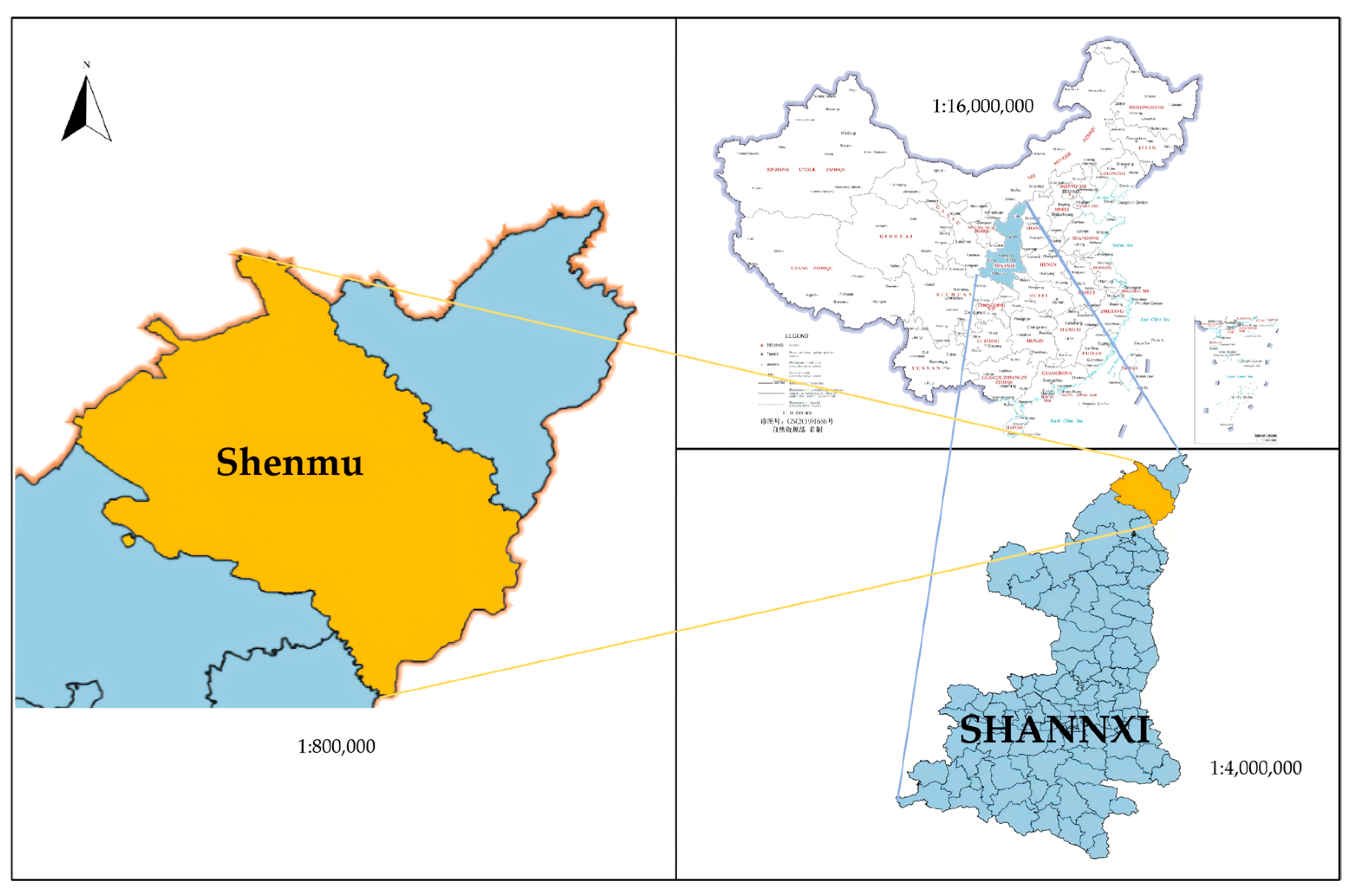
Shenmu is located in northern Shaanxi Province, encompassing a total area of 7635 km², and constituting the largest county-level administrative unit in Shaanxi Province (Figure 1). The study area occupies the transition zone between the Loess Plateau and the Mu Us Sandy Land, bisected by the Yellow River and the Great Wall. The northern wind-sand grassland and the southern hilly-gully terrain account for 51% and 49% of the total land area, respectively, functioning as the resource development zone and ecological conservation zone [40]. The region exhibits a typical arid-to-semi-arid continental climate, with an annual average precipitation of 439 mm and evaporation of 1338 mm, resulting in severe water scarcity that fundamentally limits vegetation growth and forest carbon-sink expansion.

As a national-level energy and chemical industrial base, Shenmu had a permanent population of over 580,000 (2024), annual coal output of 340 million tons, and GDP exceeding 250 billion yuan. Its economic structure is highly dependent on coal mining and heavy chemical industries, leading to extremely high carbon emissions, strong industrial lock-in, and fragile ecological conditions. This coexistence of high-carbon development pressure and water-ecological constraints makes Shenmu a typical representative case for studying carbon-neutrality pathways in resource-dependent counties in semi-arid regions.

2.2. Data Sources and Processing

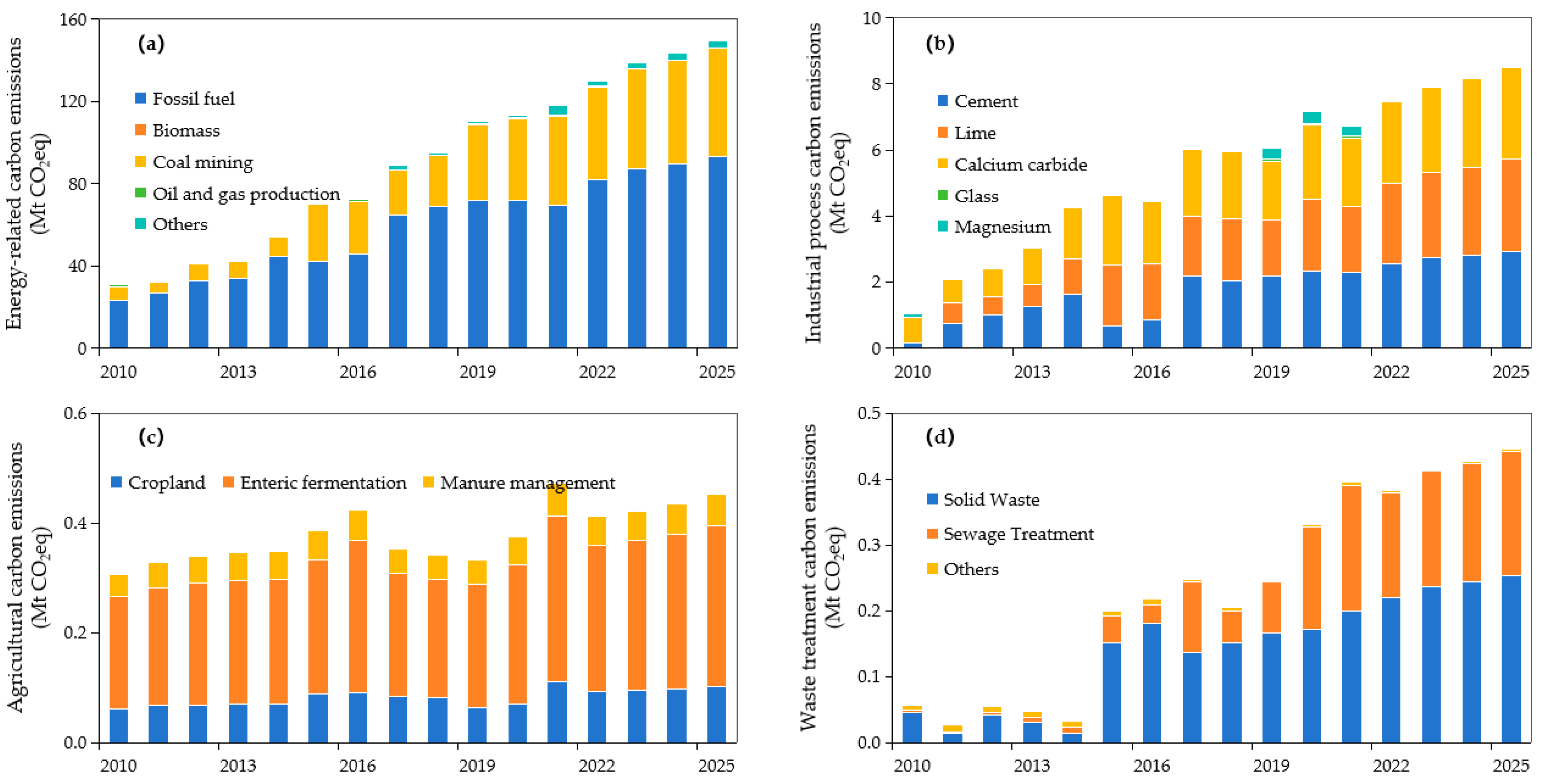
This study takes Shenmu as the accounting boundary, covering four major emission sectors: energy activities, industrial processes, agricultural activities, and waste treatment. Forest carbon sinks are assessed separately under the land use and forestry boundary. Time-series data (2010–2025) on population, GDP, energy consumption, forest resources, and land use change and forestry were collected from Shenmu Statistical Yearbooks, Shaanxi Provincial Greenhouse Gas Inventories, municipal statistical bulletins, and official releases from the local Bureau of Ecology and Environment and Forestry Bureau.

Carbon emissions were calculated following the 2006 IPCC Guidelines for National Greenhouse Gas Inventories [41,42]. Although this study follows the IPCC accounting framework at the county scale, recent integrated assessment studies have increasingly emphasized that carbon accounting systems are closely coupled with broader resource–environment–economic processes, where water use, energy consumption, and economic output jointly shape the overall sustainability performance of regional systems [43]. Although the present study focuses on territorial carbon accounting, recent life-cycle assessment studies have increasingly emphasized the interdependence among carbon emissions, water consumption, and economic performance within coupled socio-environmental systems. Such integrated analytical frameworks provide useful conceptual references for understanding regional sustainability transitions beyond conventional emission inventories. Following provincial guidelines for greenhouse gas inventory-preparation, annual emissions across four major source sectors were estimated by multiplying activity data by corresponding emission factors. The formula is:

$$E_{total}=\sum _i({AD}_i\times {EF}_i)$$

where E_total is the total greenhouse gas emissions (tCO₂eq); AD_i is the activity level of the emission source i (e.g., coal consumption); and EF_i is the corresponding emission factor, integrating net calorific value, carbon content per unit calorific value, and combustion oxidation efficiency.

The emission factors follow the 2006 IPCC Guidelines together with the provincial inventory-preparation guidelines, which provide partial regional calibration; fully localized factors for Shenmu’s specific coal quality and individual industrial processes were not available, and national/provincial defaults were therefore used. Because the net calorific value and carbon content of local coal can differ modestly from the defaults, the absolute emission totals carry a corresponding factor-level uncertainty; however, this study’s structural conclusions—the dominance of energy activities (>90%) and the order-of-magnitude emission–sink disparity—depend on relative magnitudes and are robust to this uncertainty.

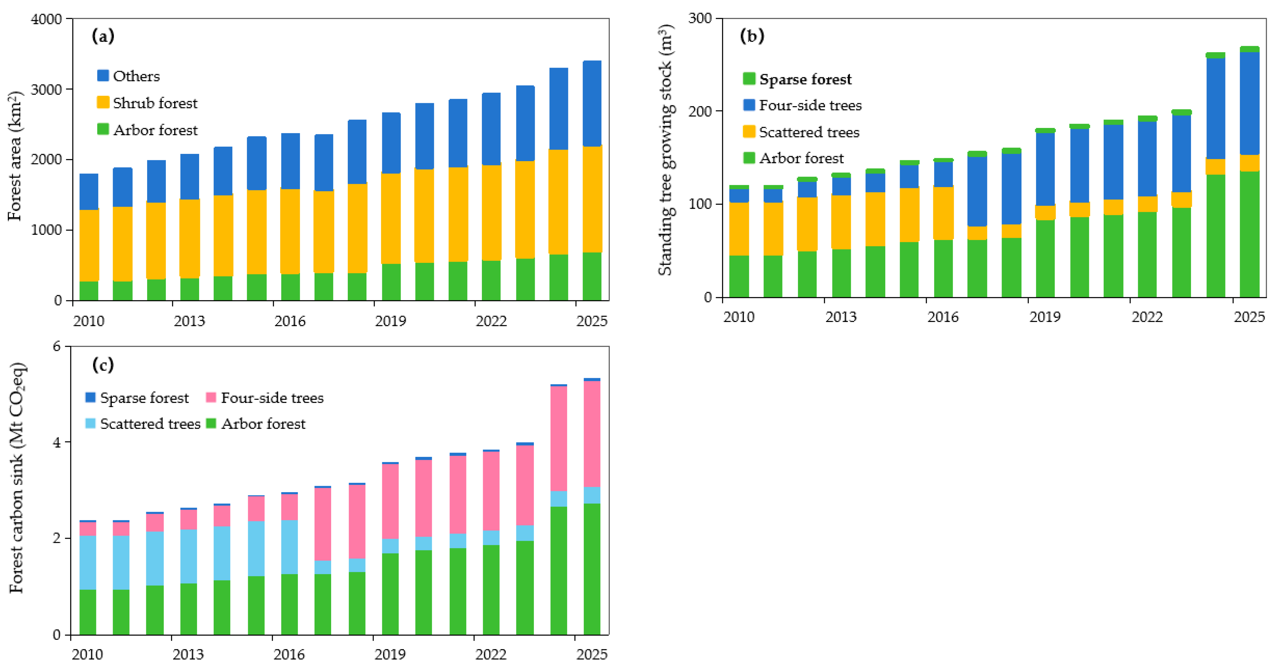
Forest carbon sinks were calculated using the forest growing-stock method [26]. The assessment is restricted to forest ecosystems only, including arbor forests, economic forests, and shrublands, and does not cover grasslands, wetlands, croplands, or other non-forest carbon pools. The calculation uses growing stock as the core input and combines it with wood density, biomass expansion factors (BEF), and carbon fraction (CF) to quantify above- and below-ground biomass carbon. Litter and soil organic carbon pools are excluded, consistent with the scope of forest carbon accounting in official inventories. All parameters take national default values (

Table A1. Forest carbon-sink accounting parameters for Shenmu.

Parameter	Description	Value
GR	Growing rate of standing stock	4.10%
CR	Consumption rate of standing stock	2.28%
SVD	Specific wood density	0.558 t·m−3
BEF (above ground)	Aboveground biomass expansion factor	1.947
BEF (below ground)	Belowground biomass expansion factor	1.517
B_bamboo	Stand biomass of bamboo forest	68.48 t·km−2
B_economic	Stand biomass of economic forest	3521 t·km−2
B_shrub	Stand biomass of shrub forest	17.99 t·km−2
CF	Carbon fraction	0.5

).

2.3. Carbon Emission Prediction Model

This study applies an extended STIRPAT model to project multi-scenario carbon emissions in Shenmu. The STIRPAT framework relaxes the proportionality constraint of the classical IPAT model and accommodates the non-linear emission dynamics characteristic of resource-based cities [44]. The baseline formula is:

$$I=a{·P}^b\times A^c\times T^d\times e$$

where I is total carbon emissions; a is a scaling constant; P, A, and T denote population, affluence, and technology, respectively; b, c, and d are their respective elasticity coefficients; and e is a stochastic error term.

Based on the structural characteristics of Shenmu, including coal dependence, high energy consumption, and a heavy industrial mix, the model is extended to incorporate six key driving factors: population size (P), per capita GDP (PGDP), energy intensity (EC), energy structure (ES), electricity consumption intensity (EI), and secondary industry share (IS). The formula is:

$$I=a·P^b\times PGD{P}^c\times E{C}^d\times E{S}^e\times E{I}^f\times I{S}^g\times e$$

2.3.1. Data and Multicollinearity Diagnostics

This study uses annual time-series data (2010–2025) rather than panel data. All variables are log-transformed, with lnI as the dependent variable and lnP, lnPGDP, lnEC, lnEI, lnES, and lnIS as explanatory variables within the extended STIRPAT framework. Pearson correlation analysis was conducted first to examine the relationships among explanatory variables. Several explanatory variables exhibit relatively high pairwise correlations (

Table A2. Correlation test of variables.

Variable	lnI	lnP	lnPGDP	lnEC	lnEI	lnES	lnIS
lnI	1	0.99	0.91	−0.09	0.92	−0.90	0.72
lnP	0.99	1	0.91	−0.11	0.89	−0.88	0.73
lnPGDP	0.91	0.91	1	−0.26	0.77	−0.75	0.83
lnEC	−0.09	−0.11	−0.26	1	0.03	−0.06	−0.63
lnEI	0.92	0.89	0.77	−0.03	1	−0.94	0.59
lnES	−0.90	−0.88	−0.75	−0.06	−0.94	1	−0.61
lnIS	0.72	0.73	0.83	−0.63	0.59	−0.61	1

), indicating the potential presence of multicollinearity and justifying further diagnostic testing. To ensure conceptual consistency in long-term scenario projections, all model variables are categorized into three distinct types.

(i)

Statistically, estimated elasticities, including population (P), per capita GDP (PGDP), and energy consumption (EC)-related variables, are derived from the RR based on historical observations (2010–2025). These parameters capture empirically observed associational relationships between socio-economic drivers and emissions within the study period.

(ii)

Scenario-driven structural variables, including energy structure (ES) and industrial structure (IS), are retained as explanatory variables in the RR estimation, yielding historically grounded elasticity coefficients (

Table 1. Ridge regression estimation results.

Variable	Non-Standardized Coefficient		Standardized Coefficient	t-Test	Significance
	B	Standard Error	Beta
a	2.417	4.453	-	0.543	0.600
lnP	1.329	0.618	0.273	2.150	0.060
lnPGDP	0.515	0.187	0.339	2.752	0.022
lnEC	0.500	0.301	0.173	1.659	0.132
lnEI	0.685	0.339	0.243	2.023	0.074
lnES	−0.470	0.396	−0.148	−1.186	0.266
lnIS	−0.013	0.850	−0.002	−0.015	0.988
R2	0.920
Adjusted R2	0.860
F	F = 16.31, p = 0.000 ***

Notes: *** indicates statistical significance at p < 0.001 level.

). However, in long-term scenario projections (2026–2060), their future trajectories are specified exogenously based on policy targets and structural transition pathways, rather than being extrapolated from their estimated historical elasticities. This distinction recognizes that these variables undergo planned structural breaks incompatible with historical trend extrapolation, and therefore embed future policy and technological transformation expectations.

(iii)

Derived intensity indicators, such as energy intensity (EI), reflect underlying structural relationships between economic output and electricity use rather than acting as independent causal drivers. Although EI enters the ridge specification empirically (Table 1; B = 0.685, β = 0.243), it is interpreted as a composite intensity indicator rather than an independent structural driver. As such, EI is interpreted as a composite indicator rather than a standalone explanatory variable.

This classification ensures that statistical estimation, scenario design, and derived structural representation are clearly separated, avoiding inconsistent interpretation of elasticity parameters in long-term projections. Ordinary least squares (OLS) estimation is first applied as the baseline specification. Multicollinearity diagnostics based on variance inflation factors (VIFs) (

Table A3. Ordinary least squares (OLS) collinearity diagnostics.

Variable	Non-Standardized Coefficient		Standardized Coefficient	t-Test	Significance	Collinearity Statistics
	B	Standard Error	Beta		p	Tolerance	VIF
a	6.66	12.47	-	0.53	0.61	-	-
lnP	2.21	1.41	0.45	1.57	0.15	0.10	9.74
lnPGDP	0.88	0.45	0.58	1.98	0.08	0.10	10.19
lnEC	0.53	0.56	0.18	0.94	0.37	0.23	4.43
lnEI	0.31	0.86	0.11	0.37	0.72	0.09	10.86
lnES	−0.39	0.81	−0.12	−0.49	0.64	0.13	7.65
lnIS	−1.94	2.56	−0.26	−0.76	0.47	0.07	14.52

) confirm severe collinearity among explanatory variables, with several VIF values exceeding conventional thresholds. This condition renders OLS estimates unstable and unsuitable for reliable elasticity estimation.

To address multicollinearity, principal component regression (PCR) and ridge regression (RR) are implemented and compared. PCR eliminates collinearity by constructing orthogonal principal components; however, this transformation removes the direct economic interpretation of individual explanatory variables. In contrast, RR stabilizes coefficient estimation while retaining the original variable structure, ensuring interpretability within the STIRPAT elasticity framework. Comparative results (

Table A4. Comparison of ridge regression (RR) and principal component regression (PCR) estimates.

Variable	Ridge Regression (RR)		Principal Component Regression (PCR)
	B	Beta	B	Beta
a	2.417	-	2.382	-
lnP	1.329	0.273	1.287	0.265
lnPGDP	0.515	0.339	0.502	0.331
lnEC	0.500	0.173	0.468	0.168
lnEI	0.685	0.243	0.672	0.239
lnES	−0.470	−0.148	−0.458	−0.145
lnIS	−0.013	−0.002	−0.011	−0.002
R2	0.920		0.917
Adjusted R2	0.860		0.852
F	F = 16.31, p = 0.000 ***		F = 15.87, p = 0.000 ***

Notes: *** indicates statistical significance at p < 0.001 level.

) support RR as the preferred specification. Accordingly, RR is adopted as the final estimation method.

The ridge-regression-based extended STIRPAT equation is expressed as:

$$\ln I=\mathrm{a}+\mathrm{b}\mathrm{l}\mathrm{n}P+\mathrm{c}\mathrm{l}\mathrm{n}PGDP+\mathrm{d}\mathrm{l}\mathrm{n}\mathrm{E}C+\mathrm{e}\mathrm{l}\mathrm{n}\mathrm{E}S+\mathrm{f}\mathrm{l}\mathrm{n}\mathrm{E}I+\mathrm{g}\mathrm{l}\mathrm{n}\mathrm{I}S$$

2.3.2. Ridge Regression and Model Validation

The optimal ridge parameter (k = 0.109) was determined via ridge trace analysis combined with generalized cross-validation. Bootstrap resampling was performed to generate corrected p-values and 95% confidence intervals, as RR yields biased estimates without classical OLS p-values (Table 1).

The ridge-regression-based extended STIRPAT model explained 0.92 of the variance in emissions (adjusted R² = 0.86) and was jointly significant (F = 16.31, p < 0.001; Table 1). Among the standardized coefficients, PGDP had the largest magnitude (β = 0.339), followed by P (β = 0.273) and EC (β = 0.243); EI showed a weaker positive association (β = 0.173), the ES entered with a negative sign, and the IS was negligible. All coefficient signs were stable across the bootstrap replications and the stepwise and partial-least-squares cross-checks, although the individual t-tests were conservative owing to the variance–bias trade-off inherent in RR.

2.3.3. Multicollinearity Diagnostics and Elasticity Interpretation

To address potential endogeneity in the population elasticity, a Frisch–Waugh–Lovell partial-correlation test is conducted. lnP is first regressed on a linear time trend, and lnI (emissions) is regressed on all remaining STIRPAT variables. The correlation between the resulting residuals is r = −0.554 (p = 0.026), indicating a statistically significant conditional association between population and emissions after controlling for confounders and temporal effects. The negative sign reflects offsetting structural processes in resource-based cities, where population inflows co-occur with industrial expansion and efficiency improvements. Accordingly, the estimated population elasticity should be interpreted as a composite structural parameter rather than a marginal causal effect. Given the limited sample size (2010–2025), instrumental-variable or time-varying coefficient approaches are not statistically reliable. Therefore, the parameter is treated as associative rather than causal, and this limitation is explicitly acknowledged.

The formula derived from the RR estimation results is:

$$\mathrm{l}\mathrm{n}I=2.417+1.329\mathrm{l}\mathrm{n}P+0.515\mathrm{l}\mathrm{n}PGDP+0.500\mathrm{l}\mathrm{n}EC+0.685\mathrm{l}\mathrm{n}EI-0.470\mathrm{l}\mathrm{n}ES-0.013\mathrm{l}\mathrm{n}IS$$

Coefficients represent emission elasticities. The partial correlation analysis based on the Frisch–Waugh–Lovell decomposition confirms a statistically significant association between population and emissions after controlling for other drivers and time trends. The population elasticity should be interpreted as a long-run scale effect rather than a causal structural parameter, reflecting the joint dynamics between population growth and industrial expansion in a resource-dependent economy. It should be noted that the positive elasticity of energy intensity does not imply that improvements in energy efficiency increase carbon emissions. During 2010–2025, declining energy intensity coincided with rapid growth in PGDP and industrial activity, resulting in strong multicollinearity among explanatory variables. Under the RR, part of the explanatory power associated with economic expansion is redistributed to the EC through coefficient regularization. Therefore, the positive coefficient should be interpreted as a statistical attribution effect within a correlated system rather than as an independent causal relationship.

2.3.4. Small-Sample Uncertainty

Given the short time series (2010–2025), extrapolation to 2060 introduces inherent uncertainty. Bootstrap 95% confidence intervals (±8.5% for the 2060 projection) and leave-one-out cross-validation are reported to characterize this scenario-dependent uncertainty.

Due to the absence of region-specific process-based ecosystem model outputs for the study area under consistent scenario assumptions, the growing-stock growth rates are parameterized using literature-constrained ranges combined with observed water limitation indicators, including precipitation, NDVI saturation trends, and soil moisture constraints.

2.3.5. Multi-Scenario Setting and Calibration

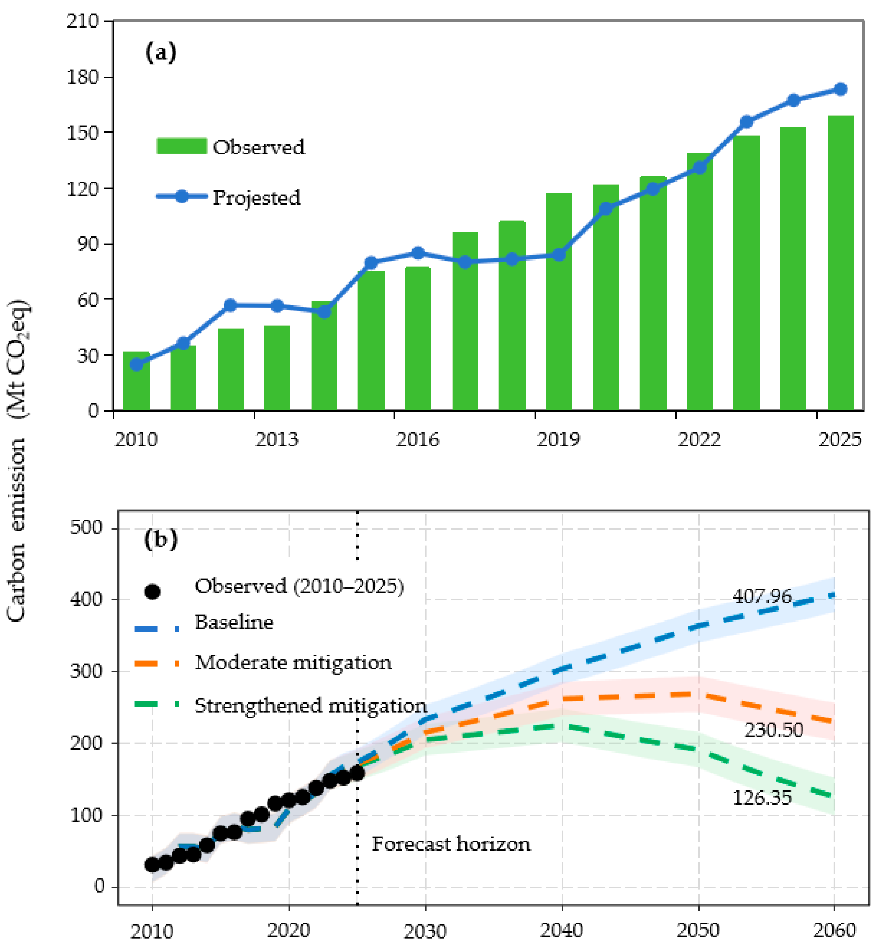
Scenario analysis assigns phased predicted values to STIRPAT variables based on historical trends, policy plans, and development expectations [45,46,47]. This ensures consistency with Shenmu’s actual socioeconomic trajectory. This study spans five phases (2010–2020, 2021–2030, 2031–2040, 2041–2050, 2051–2060) under three scenarios: baseline mitigation, moderate mitigation, and strengthened mitigation.

The scenario design isolates the policy levers most relevant to a coal-based economy. Across all three scenarios, the 2010–2020 stage reproduces observed historical growth rates and therefore coincides; the scenarios diverge only from 2021 onward. The baseline largely extends historical momentum—EC declines only marginally (−0.01 yr⁻¹) and EI continues to rise—so emissions keep growing. The moderate and strengthened scenarios progressively accelerate the decline of the two most decisive levers, energy intensity and the ES: EC falls to −0.06 yr⁻¹ after 2040, and population contracts more rapidly under the strengthened scenario (−0.04 yr⁻¹ by 2051–2060). PGDP growth is held positive throughout to honor the energy-security and economic-continuity constraints binding on a national energy base, so mitigation is achieved through structural and efficiency channels rather than through suppressed output.

Although the elasticities are held constant across 2026–2060, the scenario framework imposes time-varying exogenous growth rates on every driver (

Table 2. Temporal growth rates of key carbon emission drivers under the baseline, moderate, and strengthened mitigation scenarios in Shenmu (2026–2060).

Scenario	Stage	P	PGDP	EC	EI	ES	IS
Baseline	2010—2020	0.023	0.064	0.097	0.072	−0.023	0.004
	2021—2030	0.005	0.02	−0.01	0.05	−0.03	−0.02
	2031—2040	−0.02	0.02	−0.01	0.05	−0.03	−0.02
	2041—2050	−0.025	0.03	−0.01	0.04	−0.03	−0.02
	2051—2060	−0.03	0.04	−0.01	0.04	−0.02	−0.02
Moderate mitigation	2010—2020	0.023	0.064	0.097	0.072	−0.023	0.004
	2021—2030	−0.005	0.04	−0.03	0.05	−0.03	−0.01
	2031—2040	−0.02	0.04	−0.04	0.04	−0.02	−0.01
	2041—2050	−0.025	0.05	−0.06	0.03	−0.02	−0.01
	2051—2060	−0.03	0.05	−0.06	0.02	−0.01	−0.01
Strengthened mitigation	2010—2020	0.023	0.064	0.097	0.072	−0.023	0.004
	2021—2030	−0.01	0.04	−0.03	0.05	−0.03	−0.01
	2031—2040	−0.02	0.04	−0.04	0.04	−0.02	−0.01
	2041—2050	−0.03	0.05	−0.06	0.03	−0.02	−0.01
	2051—2060	−0.04	0.05	−0.06	0.02	−0.01	−0.01

Notes: P, population; PGDP, per capita GDP; EC, energy intensity; EI, electricity intensity; ES, energy structure; IS, secondary industry share.

), so a substantial part of the expected structural transformation is captured through the trajectories of the inputs rather than through the elasticities themselves. Constant-elasticity STIRPAT is the standard for long-horizon projection because reliable identification of time-varying coefficients is not feasible from a 16-year series. The direction of the resulting bias is, moreover, conservative for the mitigation scenarios: if deep decarbonization makes the energy structure elasticity more negative after 2050, emissions would fall faster than projected, and the strengthened scenario would peak earlier, whereas an expansion of coal-to-chemicals pathways would weaken this elasticity and widen the gap. Under the present specification, the mitigation-scenario emissions should therefore be regarded as a conservative (upper-bound) estimate of the achievable reductions.

2.4. Forest Carbon-Sink Prediction Model

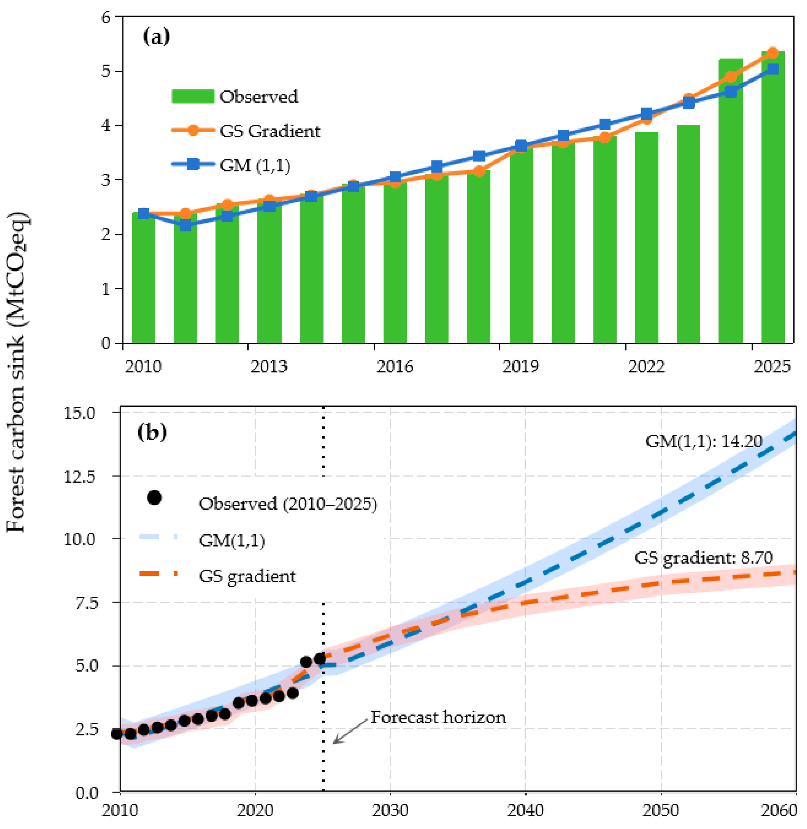
To improve the reliability of forest carbon-sink projections under semi-arid water constraints and small-sample conditions, two independent prediction models are developed and cross-validated in this study. To avoid overreliance on R², which can be inflated in monotonic small samples, we further assessed the GM(1,1) model using a precision grading system.

2.4.1. Growing-Stock Gradient Extrapolation Model

This model serves as the primary forecasting approach, leveraging the approximately linear correlation between forest growing stock and carbon flux. Phased gradient growth rates are calibrated based on historical trends (2010–2025), municipal afforestation plans, and ecological restoration targets. Carbon sink potential is subsequently calculated using BEF, specific wood density (SVD), and carbon fraction (CF) [48].

In ecosystem carbon-sink estimation, remote sensing and machine learning approaches have been increasingly applied to improve the spatial characterization of vegetation and land surface properties. For example, hyperspectral-based interpretable convolutional neural network methods can extract fine-grained spectral features and enhance environmental parameter inference in heterogeneous landscapes [49]. However, such approaches typically require high-quality remote sensing inputs and are less robust in long-term county-scale time-series reconstruction, particularly in data-scarce semi-arid regions such as the Loess Plateau. Therefore, they are used here only as a methodological reference rather than as a primary modeling tool.

It must be explicitly stated that the phased, declining forest growth rates (3.81% to 0.50%) implemented across our scenario matrix are not mathematically derived from mechanistic process-based model simulations. Instead, to maintain methodological alignment with county-scale socioeconomic projection units where grid-based process models cannot be seamlessly harmonized, these parameters are expert-elicited and empirically calibrated.

To capture the long-term dynamics of forest expansion and accumulation, we established a phased growth trajectory for both forest area and growing stock volume from 2010 to 2060. This parameterization constitutes a water-constrained macro-ecological proxy framework. The precise numerical parameters within this sequence were determined by expert consensus, which dynamically downscaled the unconstrained macro-statistical baseline trajectories over time to incorporate advancing stand age, canopy closure, and regional hydroclimatic thresholds (mean annual precipitation of 350–500 mm). To benchmark the scientific validity of this expert parameterization, we compared our growth trajectory against independently reported forest productivity metrics for the semi-arid Loess Plateau and analogous dryland ecosystems. Synthesis literature indicates that the sustainable, water-limited productivity growth of these ecosystems typically scales within a boundary of 0.3~6.0%·yr⁻¹, depending tightly on stand cohort maturity and soil moisture deficit accumulation [10]. As compiled in the expanded

Table 3. Observed historical (2010–2020) and scenario-based projected (2021–2060) growth rates of forest area and growing stock volume under water-limited constraints.

Period	Forest Area Growth (%·yr−1)	Growing Stock Growth (%·yr−1)	Dominant Influencing Factors	Literature-Supported Growth Envelope (%·yr−1)	Consistency Assessment	References
2010–2020	5.13	5.13	Large-scale ecological restoration and afforestation expansion	Upper-growth stage (>4%)	Consistent with observed rapid expansion phase	This study
2021–2025	3.81	3.81	Young stands, continuing afforestation, management improvement	Moderate-to-high growth (3–5%)	Within reported range for actively developing plantation systems	This study, [50]
2026–2030	3.11	3.11	Increasing stand age, reduced suitable afforestation land	Moderate growth (2–4%)	Consistent with transition from expansion to maturation	[50,51]
2031–2035	2.26	2.26	Canopy closure, declining marginal restoration benefits	Moderate growth (1–3%)	Consistent with maturing plantation forests	[10,50]
2036–2040	1.50	1.50	Resource constraints and productivity deceleration	Low-to-moderate growth (1–2%)	Consistent with ecological maturation trends	[10,52]
2041–2050	1.00	1.00	Approaching ecological carrying capacity	Low growth (0.5–1.5%)	Consistent with mature semi-arid forest systems	[10,53]
2051–2060	0.50	0.50	Maintenance-stage forest growth under long-term constraints	Maintenance growth (0–1%)	Conservative lower-bound estimate	[10,53]

Note: Both the historical and the future projected stages assume identical growth rates for forest area and growing stock volume within each specific envelope to maintain cross-scenario parameter consistency.

, our parameterized growth cascade transitions smoothly from an active afforestation rate toward the lower bound of the independent ecological envelope in the final stages (2051–2060), conforming to the principle of conservative carbon-sink projection under strict water resource carrying capacity limitations. Nonetheless, we explicitly acknowledge this expert-elicited parameter setting as a key structural uncertainty in our model predictions, which warrants caution during long-term extrapolation.

2.4.2. GM(1,1) Prediction Model

Given the scarcity of county-level forestry time-series data, the GM(1,1) model is adopted as an independent alternative pathway [26,54,55]. The model attenuates stochastic fluctuations via first-order accumulated generation, fits a differential equation to capture carbon-sink evolution, and reconstructs predictions through inverse accumulation. It requires minimal data and distributional assumptions, making it suitable for small-sample ecological forecasting. Forecasting performance was assessed using the gray-model criteria (posterior-error ratio and small-error probability, p = 0.98), indicating a high-precision grade.

2.5. Uncertainty and Sensitivity Analysis

Uncertainties in carbon emission and carbon sink accounting were quantified following the 2006 IPCC Guidelines and provincial inventory specifications. For activity data, emission factors, and sectoral coefficients, relative errors were estimated using standard error propagation methods based on sample means, standard deviations, and t-distribution critical values, and reported at the 95% confidence level (

Table A5. Uncertainty analysis.

Year	Energy-Related (%)	Industrial Process (%)	Agricultural (%)	Waste Treatment (%)	Land Use and Forestry (%)	Overall (%)
2010	15.15	6.22	36.39	19.52	11.41	45.87
2011	17.29	6.67	36.18	19.23	10.99	46.29
2012	19.38	7.41	35.86	18.98	10.38	46.74
2013	21.67	7.01	35.96	18.55	10.54	47.61
2014	19.33	7.73	35.90	20.22	10.17	47.27
2015	13.76	13.66	31.90	28.31	53.94	71.45
2016	12.86	12.85	32.81	30.55	39.84	62.67
2017	7.80	10.48	19.12	10.92	29.54	39.09
2018	6.92	10.46	18.99	10.90	36.85	44.66
2019	6.10	14.20	21.60	6.22	34.01	43.60
2020	6.19	14.28	21.10	6.13	29.23	39.74
2021	5.76	14.32	18.41	5.89	28.93	38.06
2022	3.47	15.63	13.78	6.72	25.12	33.50
2023	2.05	16.42	11.30	5.24	22.27	30.41
2024	1.85	17.15	10.85	5.12	21.50	30.06
2025	1.68	17.80	10.85	4.95	20.80	29.78

). This component represents the inventory-level uncertainty associated with historical emissions across energy-related, industrial process, agricultural, waste treatment, and land use and forestry sectors. The total relative uncertainty of annual carbon emissions was synthesized by the root-sum-of-squares (RSS) method across five independent emission sectors, following IPCC uncertainty guidance:

$${\mathrm{U}}_{\mathrm{t}\mathrm{o}\mathrm{t}\mathrm{a}\mathrm{l}}=\sqrt{{\mathrm{U}}_{\mathrm{e}\mathrm{n}\mathrm{e}\mathrm{r}\mathrm{g}\mathrm{y}}^2+{\mathrm{U}}_{\mathrm{i}\mathrm{n}\mathrm{d}\mathrm{u}\mathrm{s}\mathrm{t}\mathrm{r}\mathrm{y}}^2+{\mathrm{U}}_{\mathrm{a}\mathrm{g}\mathrm{r}\mathrm{i}}^2+{\mathrm{U}}_{\mathrm{w}\mathrm{a}\mathrm{s}\mathrm{t}\mathrm{e}}^2+{\mathrm{U}}_{\mathrm{l}\mathrm{u}\mathrm{l}\mathrm{u}\mathrm{c}\mathrm{f}}^2}$$

where U_i corresponds to the sector-specific relative uncertainty (%) for energy combustion, industrial processes, agricultural activities, waste treatment, and land use, land-use change and forestry, respectively. Year-by-year sectoral uncertainty data and the corresponding aggregated overall uncertainty results are fully documented in Table A5.

The carbon-neutrality gap is a derived quantity equal to the difference between emission and sink projections, each carrying independent uncertainty of different distributional origin. Propagating these separate uncertainties into a joint confidence interval for the gap requires Monte Carlo simulation rather than simple interval arithmetic. To capture model-level uncertainty, the GM(1,1) model was used to characterize emission projection uncertainty and the GS gradient model was used to characterize forest carbon-sink uncertainty, with confidence intervals derived from bootstrap prediction intervals (

Table A8. Bootstrap 95% prediction intervals for GS gradient and GM(1,1) forest carbon sink, 2030–2060 (MtCO₂eq).

Year	GS Gradient Model			GM(1,1) Model
	Forecast	Lower 95% PI	Upper 95% PI	Forecast	Lower 95% PI	Upper 95% PI
2030	6.22	5.72	6.54	5.91	5.49	6.51
2035	6.95	6.46	7.27	7.07	6.65	7.67
2040	7.49	6.99	7.81	8.31	7.89	8.90
2045	7.87	7.38	8.19	9.64	9.21	10.23
2050	8.28	7.78	8.60	11.06	10.63	11.65
2055	8.49	7.99	8.81	12.57	12.15	13.17
2060	8.70	8.20	9.02	14.20	13.77	14.79

). To incorporate additional sources of forest-sink uncertainty—including post-2020 accounting variability and long-term trend extrapolation—a composite uncertainty envelope was applied, encompassing rather than supplementing the model-structural interval. A Monte Carlo simulation with 50,000 iterations was implemented [56,57], jointly perturbing emission and sink projections within their respective uncertainty distributions in each iteration to generate the full probability distribution of the carbon-neutrality gap.

2.6. Definition of Carbon-Neutrality Gap

The carbon-neutrality gap is defined as the annual residual carbon emissions that cannot be offset by available carbon sinks, representing the core quantitative indicator for assessing the low-carbon transition pressure in resource-based cities [58,59]. Mathematically, the gap is expressed as:

$$G_{apt}=E_t-(S_t^F+S_t^G+S_t^S+S_t^{CCUS})$$

where G_apt is the carbon-neutrality gap in year t (MtCO₂eq); E_t is total anthropogenic carbon emissions (energy, industry, agriculture, and waste); ${\mathrm{S}}_{\mathrm{t}}^{\mathrm{F}}$ is forest carbon sinks (quantified in this study); ${\mathrm{S}}_{\mathrm{t}}^{\mathrm{G}}$ is grassland carbon sinks; ${\mathrm{S}}_{\mathrm{t}}^{\mathrm{S}}$ is soil organic carbon sinks; and ${\mathrm{S}}_{\mathrm{t}}^{\mathrm{C}\mathrm{C}\mathrm{U}\mathrm{S}}$ is carbon capture, utilization, and storage removal.

The equation is the general conceptual definition of the carbon-neutrality gap. In the empirical accounting of the baseline and moderate scenarios, the S_t^G and S_t^S terms are set to zero owing to the absence of consistent county-level data; this omission is quantified in Section 4.2.2 and shown to widen the gap by less than 8%, thereby biasing the estimate conservatively, and the S_t^CCUS is non-zero only under the strengthened scenario. The S_t^F is thus the only sink evaluated in the baseline and moderate scenarios, and the framework remains internally consistent in that every term retained in the operational accounting is explicitly quantified.

In accordance with the methodology framework for forest carbon-sequestration afforestation projects, this study only accounts for forest carbon sinks (${\mathrm{S}}_{\mathrm{t}}^{\mathrm{F}}$) within the official greenhouse gas inventory boundary. Grassland carbon sinks and soil organic carbon sinks are excluded from the accounting scope due to data constraints and methodological limitations. Carbon capture, utilization, and storage (CCUS) is incorporated only in the strengthened mitigation scenario to represent technological decarbonization potential in energy-intensive sectors. In this study, CCUS deployment is limited to large stationary point sources, including coal-fired power plants, coal-chemical industries, and cement production, which together account for approximately 85–88% of total energy-related emissions. Diffuse emission sources such as transportation, residential consumption, and agriculture are excluded due to limited technological applicability.

To avoid double counting, CCUS reductions were evaluated separately from the STIRPAT-based emission projections. The strengthened mitigation scenario was selected as the reference case because it represents the lowest residual-emission pathway achievable through currently available structural and technological mitigation measures. Therefore, CCUS was assessed as a complementary option for mitigating residual industrial emissions that remain after conventional decarbonization measures have been largely exhausted.

The CCUS system is parameterized using a capturable fraction of 85% (i.e., approximately 85% of total residual emissions originate from large stationary point sources technically suitable for capture), consistent with IEA assessments of post-combustion applicability. A nominal capture efficiency of 90% is subsequently applied to the capturable fraction. An energy penalty of 8–12% is explicitly incorporated into gross emissions to reflect efficiency losses and increased upstream fuel consumption. Therefore, CO₂ captured is calculated from pre-capture emissions, ensuring mass-balance consistency and avoiding double counting between capture efficiency and energy penalty effects. The detailed annual CCUS accounting, including gross emissions, energy penalty emissions, captured CO₂, and net emissions for 2030–2060 (

Table A6. Projections of carbon emissions and CCUS performance metrics from 2030 to 2060.

Year	Gross Emissions	Capturable Emissions (85%)	Captured CO2 (90%)	Energy Penalty (10%)	Net CO2 Removal	Removal Residual After CCUS
	MtCO2eq	MtCO2eq	MtCO2eq	MtCO2eq	MtCO2eq	MtCO2eq
2030	205.48	174.66	157.19	15.72	141.47	64.01
2035	215.40	183.09	164.78	16.48	148.30	67.10
2040	225.80	191.93	172.74	17.27	155.46	70.34
2045	208.00	176.80	159.12	15.91	143.21	64.79
2050	191.61	162.87	146.58	14.66	131.92	59.69
2055	155.59	132.25	119.03	11.90	107.12	48.47
2060	126.35	107.40	96.66	9.67	86.99	39.36

Note: Residual emissions are derived from the strengthened mitigation scenario presented. Capturable emissions are assumed to account for 85% of total residual emissions. A nominal capture efficiency of 90% is applied to capturable CO₂ emissions. Energy-penalty emissions are assumed to equal 10% of captured CO₂. Net CO₂ removal equals captured CO₂ minus energy-penalty emissions. Residual emissions after CCUS equal projected emissions minus net CO₂ removal.

).

2.7. Statistical Analysis

All data preprocessing, multivariate statistical modeling, uncertainty evaluation and visualization were completed using specified analytical software with complete vendor and version information: Microsoft Excel 2019 (Microsoft Corporation, Redmond, WA, USA) was applied for raw carbon emission and carbon sink dataset collation, normalization and preliminary calculation; all core quantitative analyses including ridge regression-based extended STIRPAT modeling, VIF multicollinearity diagnosis, Frisch–Waugh–Lovell partial correlation test, GM(1,1) grey prediction, bootstrap resampling and 50,000-iteration Monte Carlo uncertainty simulation were performed in R v4.2.2 (R Core Team, Vienna, Austria), with the ggplot2 package for scientific plotting, and a unified significance threshold of p < 0.05 was adopted for all hypothesis tests unless otherwise specified.

3. Results

3.1. Historical Evolution of Carbon Emissions and Carbon Sinks

Energy activities and industrial production processes accounted for the largest shares of total carbon emissions throughout the study period, whereas emissions from agriculture and waste treatment remained comparatively low. Forest carbon sinks increased over time, but their growth was substantially slower than that of carbon emissions.

Carbon emissions exhibited distinct sectoral characteristics. Energy-related emissions increased from 29.93 MtCO₂eq in 2010 to 149.38 MtCO₂eq in 2025, and consistently contributed more than 92% of total emissions (Figure 2a). Industrial process emissions contributed 3.3–7.2% of total emissions and showed a gradual upward trend (Figure 2b). Agricultural emissions fluctuated within a relatively narrow range, with cropland management and enteric fermentation remaining the two major sources (Figure 2c). Waste-treatment emissions represented the smallest component but increased steadily after 2016, mainly due to increases in landfill, sewage treatment, and waste-incineration emissions (Figure 2d). Despite their growth, the combined contribution of industrial-process and waste-treatment emissions remained relatively small compared with energy-related emissions.

Forest resources expanded steadily between 2010 and 2025 (Figure 3). The forest area increased from 1782.97 km² to 3386 km² (Figure 3a), while standing-tree growing stock rose from 1.19 × 10⁶ m³ to 2.68 × 10⁶ m³ (Figure 3b). Arbor forests contributed the largest increase in growing stock over the study period. Correspondingly, forest carbon sinks increased from 2.38 MtCO₂eq in 2010 to 5.34 MtCO₂eq in 2025, with an average annual growth rate of 5.54% (Figure 3c). After 2019, carbon-sink growth continued as forest area expansion slowed and standing-tree volume increased.

Annual carbon emissions increased from 31.32 MtCO₂eq in 2010 to 158.78 MtCO₂eq in 2025 (Figure 4). The average annual growth rate of carbon emissions was 11.43%, compared with 5.54% for forest carbon sinks. The carbon-sink offset ratio remained below 4% throughout the study period, and the difference between the total emissions and forest carbon sinks increased continuously.

3.2. Multi-Scenario Prediction of Carbon Emissions

To characterize the trajectory of carbon emissions in Shenmu from 2010 to 2060 and quantify emission reduction outcomes under varying policy intensities, the extended STIRPAT model is applied to construct three scenarios: baseline, moderate mitigation, and strengthened mitigation. Scenario parameters are calibrated in accordance with the regional positioning as an energy base, industrial structural rigidity, and national dual-carbon planning, ensuring regional applicability. The coefficient of determination R² > 0.90, and adjusted R² = 0.86 during the validation period (Figure 5a).

During 2010–2025, observed carbon emissions increased from 31.32 MtCO₂eq to 158.78 MtCO₂eq. Simulated values closely matched the observed trend throughout the validation period (Figure 5a). Under the baseline scenario, carbon emissions continued to increase throughout the projection period, reaching 407.96 MtCO₂eq in 2060 (Figure 5b;

Table A7. Bootstrap 95% prediction intervals for carbon emissions, 2030–2060 (MtCO₂eq).

Year	Baseline			Moderate Mitigation			Strengthened Mitigation
	Forecast	Lower 95% PI	Upper 95% PI	Forecast	Lower 95% PI	Upper 95% PI	Forecast	Lower 95% PI	Upper 95% PI
2030	233.88	213.48	254.33	215.76	193.59	237.70	205.48	183.45	227.36
2035	266.78	245.86	288.05	237.94	215.06	260.68	215.40	192.76	238.08
2040	304.31	282.61	325.94	262.39	238.69	286.14	225.80	202.16	249.35
2045	332.96	310.49	355.57	265.87	241.59	289.99	208.00	183.79	231.93
2050	364.30	341.17	387.40	269.39	244.18	294.27	191.61	166.82	216.53
2055	385.51	361.96	409.10	249.19	223.28	275.17	155.59	130.03	180.98
2060	407.96	383.79	432.19	230.50	204.28	256.90	126.35	100.45	152.29

). The growth rate gradually decreased after 2030, but emissions did not peak before 2060. Under the moderate mitigation scenario, emissions increased until 2050, reaching a peak value of 269.39 MtCO₂eq in 2050, and then declined to 230.50 MtCO₂eq in 2060. Under the strengthened mitigation scenario, emissions peaked before 2040 at 225.80 MtCO₂eq and subsequently declined to 126.35 MtCO₂eq in 2060. Differences among the three scenarios became increasingly evident after 2035. By 2060, the projected difference between the baseline and strengthened mitigation scenarios reached 281.61 MtCO₂eq.

3.3. Prediction of Forest Carbon-Sink Potential

Based on the observed carbon-sink series from 2010 to 2025, the GS gradient model and GM(1,1) model were calibrated and applied for future projections (Figure 6). The GS gradient model produced an R² value of 0.998, while the GM(1,1) model produced an R² value of 0.995, with only minor deviations in the early portion of the series. These results confirm that both models reliably capture the temporal dynamics of forest carbon sinks, providing a robust basis for long-term projections over 2026–2060.

Forest carbon sinks increased from 2.38 MtCO₂eq in 2010 to 5.34 MtCO₂eq under the GS gradient model and 5.03 MtCO₂eq under the GM(1,1) model in 2025 (Figure 6a). Simulated values from both models remained close to the observed series, and their 95% prediction intervals largely overlapped during the calibration period. Forest coverage was projected to increase from 44.35% in 2025 to 48.88% in 2030 (Figure 6b, Table A8). Larger differences emerged after 2035. By 2060, the GM(1,1) model projected a forest carbon sink of 14.20 MtCO₂eq, whereas the GS gradient model projected 8.70 MtCO₂eq. The difference between the two projections reached 63.2%.

3.4. Calculation of the Carbon-Neutrality Gap

Carbon-neutrality gaps under different scenarios were estimated by combining projected carbon emissions and forest carbon sinks (

Table 4. Projected carbon-neutrality gap (MtCO₂eq).

Year	Baseline Gap		Moderate Mitigation Gap		Strengthened Mitigation Gap
	Lower	Upper	Lower	Upper	Lower	Upper
2030	227.66	227.97	209.54	209.85	199.26	199.56
2040	296.00	296.82	254.08	254.90	217.48	218.30
2050	353.25	356.03	258.33	261.11	180.55	183.33
2060	393.76	399.26	216.30	221.80	112.15	117.65

Note: For each scenario, the lower and upper values bracket the carbon-neutrality gap using the two sink models: the lower bound subtracts the larger, unconstrained GM(1,1) sink, and the Upper bound subtracts the smaller, water-constrained growing-stock sink from projected emissions. Propagating the combined emission, sink, and parameter uncertainty through the gap (Monte Carlo, N = 50,000) yields a 95% interval dominated by the emission term and amounting to roughly ±9% of the gap, which lies far above zero in every scenario.

). Across all scenarios, projected carbon emissions remained substantially higher than projected forest carbon sinks throughout the study period. Under the baseline scenario, the carbon-neutrality gap increased from 227.66–227.97 MtCO₂eq in 2030 to 393.76–399.26 MtCO₂eq in 2060. Under the moderate mitigation scenario, the gap reached 216.30–221.80 MtCO₂eq in 2060. Under the strengthened mitigation scenario, the corresponding value decreased to 112.15–117.65 MtCO₂eq.

Overlaying the three emission scenarios and both sink projections on a common timeline shows that every emission trajectory (126.35–407.96 MtCO₂eq by 2060) lies far above the sink envelope (8.70–14.20 MtCO₂eq); the vertical distance between them is the carbon-neutrality gap, whose magnitude is governed far more strongly by the mitigation scenario than by the choice of sink model.

From 2010 to 2060, forest carbon sinks are projected to increase continuously, but are subject to the compounding constraints of semi-arid climate, water–soil resource carrying capacity, and finite suitable forest land, imposing a rigid ecological ceiling on carbon-sink expansion. For a short time, carbon-sink growth relies primarily on forest land expansion before 2025; after 2025, the growth rate decelerates substantially, as the focus shifts to stand structure optimization and quality improvement. From a carbon-balance perspective, projected 2060 emissions exceed forest carbon sinks by roughly 15-fold under strengthened mitigation and by up to 47-fold under the baseline (Table 4), so natural carbon sinks remain structurally incapable of offsetting fossil-energy emissions on their own. Propagating the combined uncertainty through the gap gives a 2060 baseline gap of 396 ± 35 MtCO₂eq, so the gap remains significantly positive under every scenario. Under the baseline scenario, emissions continued to rise without peaking before 2060. Moderate and strengthened mitigation scenarios substantially reduce future emissions, yet residual emissions remained considerable. Forest carbon sinks are projected to increase steadily under both the GS gradient and GM(1,1) models, but growth is constrained by limited afforestation potential and water–soil resource availability. As a result, projected sink capacity offset approximately 2.1–11.2% of total emissions by 2060, depending on the emission scenario and sink model adopted.

4. Discussion

4.1. Structural Carbon-Neutrality Constraints in Resource-Based Cities

Shenmu is a representative coal-dominated county within China’s national energy production system. Wang et al. [60] reported that coal-dependent resource-based cities generally show lower transition resilience because economic activities remain strongly linked to fossil-energy industries. Such regions are often classified as structurally constrained transition systems, where industrial lock-in and resource dependence exert stronger influences on transition outcomes than marginal policy adjustments. This perspective further supports the classification of Shenmu as a high-lock-in system.

As one of China’s major coal-producing counties, Shenmu remains highly dependent on coal mining and coal-chemical industries. This industrial structure slows the decoupling of economic growth from carbon emissions and contributes to the persistence of high emission levels [3,61]. Compared with manufacturing-oriented cities, emission reduction in energy-producing regions is more strongly influenced by resource endowment and industrial specialization.

The comparison presented in

Table 5. Comparative carbon-neutrality constraints among representative coal-dominated resource-based cities in China (2023).

City	Total Carbon Emissions (MtCO2eq)	Forest Carbon Sinks (MtCO2eq)	Carbon-Sink Offset Ratio (%)	References
Yulin, Shaanxi	192.34	19.12–40.91	9.94–21.27	[62,63]
Ordos, Inner Mongolia	284.43	19.12–40.91	6.72–14.38	[62,63]
Shuozhou, Shanxi	74.35	0.01–19.12	0.01–25.72	[62,63]
Changzhi, Shanxi	72.57	19.12–40.91	26.35–56.37	[62,63]
Yangquan, Shanxi	35.86	0.01–19.12	0.03–53.32	[62,63]
Jining, Shandong	81.88	0.01–19.12	0.01–23.35	[62,63]
Xuzhou, Jiangsu	95.02	0.01–19.12	0.01–20.12	[62,63]

Note: Total carbon emissions for all cities refer to the 2023 base year and are drawn from a consistent 2023 city-level CO₂ dataset. The forest-carbon-sink and offset-ratio columns are reported as ranges because the source studies adopt different sink-accounting boundaries (e.g., inclusion or exclusion of grassland and shrub pools).

further highlights these characteristics. Shenmu exhibits a lower carbon-sink offset ratio than several other coal-based cities. Although forest carbon sinks have increased steadily, their growth remains substantially smaller than the increase in anthropogenic emissions. 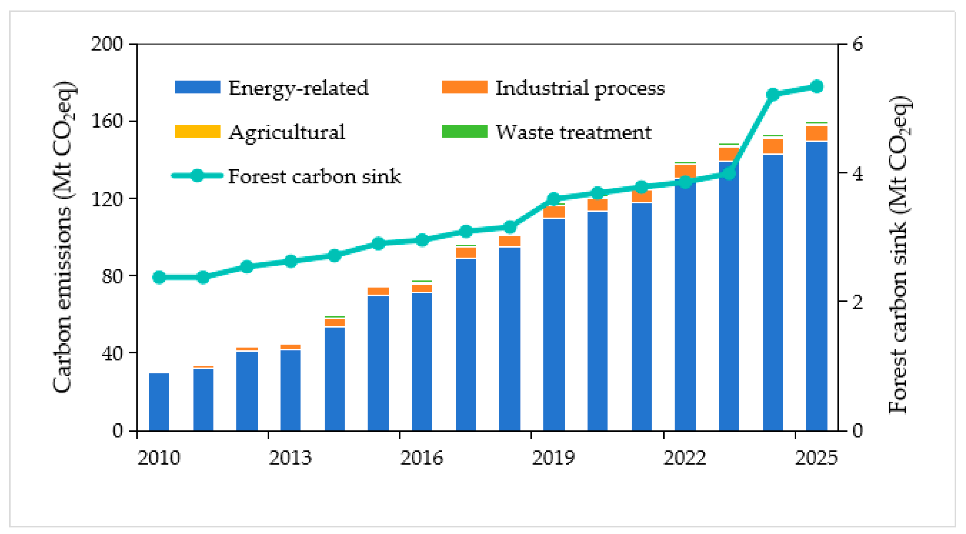Consequently, the gap between carbon sources and sinks remains larger than that reported for resource-based cities with more diversified economic structures [62,63]. Such divergence reflects a dual structural mechanism: emission intensity is amplified by coal-chemical industrial dominance, while carbon-sink capacity is constrained by limited ecological endowment and slow growth of forest carbon storage. This mismatch indicates that carbon neutrality is not constrained by emissions alone, but by the asymmetry between emission expansion and ecological absorption capacity.

This structural dependence substantially limits the short-term effectiveness of conventional mitigation measures, such as energy efficiency improvements and low-end industrial adjustments [64,65]. The rapid growth of Shenmu’s total carbon emissions over the study period far exceeds the national average growth rate, highlighting the amplified carbon burden imposed by its positioning as a national energy base [66].

The RR results provide additional insight into the factors associated with emission growth. PGDP showed the largest standardized coefficient, indicating that economic expansion remains closely linked to regional emissions [44,67,68]. Population elasticity also exceeded the range commonly reported in STIRPAT studies [44]. However, this coefficient should not be interpreted as a purely demographic effect. In Shenmu, population growth has largely accompanied coal-industry expansion, infrastructure development, and increasing energy demand. Therefore, the estimated elasticity reflects a combined scale effect of population and economic activities rather than a direct causal relationship. Similar patterns have been reported in other energy-intensive regions [69,70]. Industrial structure exhibited a comparatively small elasticity, suggesting limited short-term structural adjustment during the study period [71]. The positive coefficient of energy intensity should also be interpreted cautiously because ridge regression redistributes explanatory power among highly correlated variables. Accordingly, the estimated elasticities are better interpreted as relative associations than as independent causal effects.

Overall, the results indicate that the carbon-neutrality challenge in Shenmu arises from the combined effects of sustained emission growth and comparatively limited sink expansion. This interpretation aligns with existing case evidence: Xiong et al. [72] showed that rigid industrial composition and fossil-energy lock-in constrain low-carbon transition in resource-based cities regardless of policy effort, while Lin et al. [61] found that coal-production-based emissions in Chinese mining cities are spatially governed by resource endowment rather than efficiency alone. The present study extends these findings by quantifying the sink-side ecological ceiling that compounds emission-side rigidity, rendering the structural constraint in Shenmu doubly binding. The persistence of high-carbon lock-in reflects the combined influence of resource endowments, industrial specialization, and national spatial-functional mandates [73,74]. Within the green-transition resilience typology proposed for resource-based cities [75], Shenmu falls among the most constrained, coal-chemical-locked cases—those with the least capacity to absorb and adapt to decarbonization shocks. The projected emission trajectories are also broadly consistent with previous assessments for Shaanxi Province and comparable resource-based regions under different mitigation pathways [47].

4.2. Ecological Ceiling and Limited Offset Capacity of Natural Carbon Sinks

Forest carbon sinks are projected to increase throughout the study period, but their growth rate gradually declines after 2035. This pattern reflects the ecological characteristics of Shenmu and the broader semi-arid Loess Plateau region. Annual precipitation in Shenmu is approximately 439 mm, placing the region near the lower boundary required to sustain long-term biomass accumulation in water-limited ecosystems [76]. Feng et al. [10] have shown that vegetation restoration under such conditions may increase competition for soil water and reduce long-term growth rates.

4.2.1. Model Reconciliation and Projection Reliability

To account for these constraints, the GS gradient model incorporated progressively declining growth rates, whereas the GM(1,1) model extended historical growth trends without explicitly considering ecological limitations. Although both models reproduced historical observations well, their projections diverged after 2035. By 2060, the GM(1,1) projection exceeded the GS gradient estimate by more than 60%. This difference reflects contrasting model assumptions regarding long-term forest growth. Nevertheless, both models indicate that forest carbon sinks remain substantially smaller than projected emissions.

This divergence is structural rather than statistical: the GM(1,1) model extrapolates a constant-rate accumulation that ignores any site carrying-capacity limit [77], whereas the GS gradient model embeds the progressive deceleration of carbon increment as stands approach that limit, consistent with stand-dynamics theory [78,79]. Accordingly, the GS gradient model projection is adopted as the policy-relevant estimate and GM(1,1) as an optimistic upper bound; because even the upper bound offsets only a single-digit percentage of emissions, the policy conclusion is robust to model choice.

4.2.2. Sink Growth Dynamics and Structural Constraints

The growth of carbon sinks initially depends on forest expansion, but gradually shifts toward stand structure optimization and biomass accumulation [8,80]. However, limited precipitation, fragile soil-water systems, and finite afforestation potential constrain long-term sink expansion [10,81]. Our projections reveal that although forest carbon sinks increase substantially by 2060 relative to current levels, the offset ratio remains insufficient to achieve regional carbon neutrality independently. The mismatch between rapidly growing anthropogenic emissions and slowly saturating ecological sinks creates a widening carbon-neutrality gap during the critical 2030–2050 transition period [82].

The contribution of non-forest carbon pools was also evaluated. Grasslands and soil organic carbon were not included in the primary accounting framework because of data limitations. To assess their potential influence, an additional estimation was conducted using regional land-use data, soil organic carbon density data from the Second National Soil Survey, and published sequestration rates for the Loess Plateau [83,84]. The results suggest that the annual sink provided by non-forest ecosystems would range from approximately 0.07 to 0.33 MtCO₂eq. Even when combined with forest carbon sinks, the total natural sink remains below 9.1 MtCO₂eq yr⁻¹ [51]. Omitting these pools therefore overestimates the carbon-neutrality gap by less than 0.3% relative to the gap itself (or less than 8% relative to the forest carbon sink), confirming that the forest-focused accounting boundary is methodologically conservative and does not materially affect the central conclusions.

The findings are consistent with previous studies of ecological restoration in China. Lu et al. [85] reported that large-scale restoration programs increased regional carbon storage but offset only a limited proportion of fossil-fuel emissions. Similar conclusions were found that ecological restoration improved ecosystem carbon sequestration but could not fully compensate for emissions from energy-intensive economic activities [86,87]. The results obtained in Shenmu follow the same pattern, although the contrast between emissions and sink capacity is more pronounced because of the region’s high emission intensity and semi-arid environmental conditions. Ecological restoration alone cannot fundamentally offset rigid industrial emissions in resource-based energy regions [76]. Therefore, future carbon-neutrality pathways in semi-arid resource-based cities should emphasize diversified sink portfolios that integrate forests, grasslands, soil carbon sequestration, and technological negative-emission approaches such as CCUS and biochar enhancement [4,88].

4.3. Implications for Carbon-Neutrality Pathway Design

The persistent mismatch between rigid industrial emissions and limited ecological sink capacity implies that resource-based cities cannot rely solely on natural carbon sequestration to achieve carbon neutrality. Instead, integrated transition pathways combining industrial decarbonization, technological substitution, and market-based carbon governance are required [89]. Therefore, mitigation efforts will need to combine emission reduction and carbon removal measures.

Industrial restructuring and energy transition remain the primary approaches for controlling long-term emission growth. However, even under the strengthened mitigation scenario, a considerable residual gap remains by 2060. Carbon-market mechanisms may further support mitigation efforts by encouraging technological innovation and improving the allocation efficiency of emission-reduction resources [90,91,92,93]. For regions with limited ecological sink capacity, cross-regional carbon compensation may help alleviate local sink deficits and complement local mitigation measures [94,95,96,97]. Additionally, low-carbon technology-network analysis can map the inter-regional CCUS linkages through which an energy base connects to a broader decarbonization network [98], while accounting for the amplified water-consumption pressure that CCUS deployment imposes in arid regions [99].

Finally, this study suggests that differentiated carbon-neutrality strategies are necessary for resource-based cities with strong fossil-energy dependence. Uniform national peaking timelines may not fully account for regional functional heterogeneity, particularly in strategic energy supply zones such as Shenmu and Ordos. Future policy frameworks should therefore balance national energy security objectives with differentiated regional decarbonization pathways, recognizing that one-size-fits-all approaches may be neither feasible nor optimal for energy-based regions. A recent study of low-carbon technology collaboration networks suggests that technological diffusion and cross-sector innovation linkages play important roles in accelerating regional low-carbon transitions [100]. Therefore, CCUS deployment should be integrated with broader portfolios of energy-efficiency improvements, renewable-energy expansion, and industrial process optimization rather than being considered as an isolated mitigation measure.

4.4. Limitations and Future Research Directions

This study has several limitations. First, only forest carbon sinks were explicitly included in the accounting framework because long-term datasets for grassland and soil carbon pools were unavailable at the municipal scale. Although supplementary estimates suggest that their contribution is relatively limited, incorporating multiple ecosystem carbon pools would improve the completeness of future assessments.

Second, the extended STIRPAT model adopts constant elasticity coefficients over the entire projection horizon (2026–2060). Although time-varying growth rates are assigned to all scenario drivers, the underlying emission elasticities are held fixed at their ridge-regression estimates derived from the 2010–2025 historical period. Time-varying coefficient specifications are theoretically preferable for long-horizon projections but are not statistically feasible with a 16-year time series, as reliable parameter identification would require substantially longer observations. Additionally, the population elasticity (B = 1.329) should be interpreted as associational rather than causal, reflecting a composite scale effect of demographic and industrial expansion in a resource-dependent economy. Future panel studies spanning multiple coal-dominated cities would provide the cross-sectional variation required for causal identification of the demographic component. If deep decarbonization causes the energy-structure elasticity to become more negative after 2040—as substitution of renewables for coal accelerates—actual emissions under the strengthened scenario would fall faster than projected, meaning the present framework provides a conservative upper bound on residual emissions. Conversely, expansion of coal-to-chemicals pathways could weaken this elasticity and widen the gap. The constant-elasticity assumption therefore introduces directional uncertainty that future work with longer time series or process-based hybrid models should address.

Third, the phased forest growing-stock growth rates (3.81% declining to 0.50% yr⁻¹) were determined through structured expert consultation with specialists from the Shaanxi Academy of Forestry Sciences, the Yulin Municipal Water Resources Bureau, and the Yulin Municipal Forestry Bureau, rather than as outputs from process-based ecosystem models. Although these rates are benchmarked against the literature-supported water-limited productivity envelope for semi-arid Loess Plateau ecosystems and are consistent with reported deceleration trajectories under progressive soil moisture depletion, the absence of region-specific process-model validation means the precise growth rates carry inherent uncertainty. Alternative expert judgments within the reported envelope would shift the 2060 forest carbon-sink estimate, though not enough to alter the qualitative finding that natural sinks remain structurally insufficient to close the carbon-neutrality gap.

Fourth, CCUS was treated as a supplementary mitigation option under the strengthened mitigation scenario. The assessment incorporated capture efficiency and energy-penalty effects but did not evaluate geological storage capacity, infrastructure requirements, or economic feasibility. Consequently, the estimated mitigation contribution should be interpreted as a technical potential rather than an implementation forecast.

Future research should expand carbon accounting to include multiple ecosystem carbon pools, improve representation of hydrological constraints in semi-arid regions, and evaluate the techno-economic feasibility of CCUS deployment. Comparative studies across multiple coal-dominated energy bases would further improve understanding of regional differences in carbon-neutrality pathways.

5. Conclusions

This study integrated an extended STIRPAT model, ridge regression, and dual-model forest carbon-sink simulations to assess carbon emissions, sink dynamics, and the carbon-neutrality gap in Shenmu, a coal-dominated resource-based city on the Loess Plateau. Coupling emission projections with estimates of ecological sequestration capacity enabled a quantitative evaluation of the extent to which forest carbon sinks can offset anthropogenic emissions under alternative development pathways.

Energy-related activities dominated carbon emissions throughout the study period, consistently accounting for more than 90% of the total. Under the baseline scenario, emissions continued to rise without peaking before 2060. Moderate and strengthened mitigation scenarios substantially reduced future emissions, yet residual emissions remained considerable. Forest carbon sinks increased steadily under both the GS gradient and GM(1,1) models, but growth was constrained by limited afforestation potential and water–soil resource availability. As a result, projected sink capacity offset approximately 2.1–11.2% of total emissions by 2060, depending on the emission scenario and sink model adopted.

A persistent carbon-neutrality gap was identified across all scenarios. The projected growth of forest carbon sinks was substantially smaller than the increase in anthropogenic emissions, producing a structural long-term mismatch between carbon sources and sinks. This finding indicates that achieving carbon neutrality in coal-dominated regions requires not only emission reductions but also explicit strategies to address the inherently limited sequestration capacity of regional ecosystems.

The analytical framework developed here offers a replicable approach for evaluating carbon-neutrality pathways in resource-dependent regions. The results provide quantitative evidence that ecological constraints must be incorporated into regional carbon-neutrality assessments. Coordinating emission reduction, ecological restoration, and carbon-removal technologies remains essential to narrowing the carbon-neutrality gap in similar resource-based cities.