Indoor Air Quality Assessment in Educational Spaces Through CFD Modelling of CO₂ Distribution: Implications for Sustainable Building Design

Abstract

Indoor air quality (IAQ) plays a critical role in the health and cognitive performance of students, making its assessment essential for sustainable building design in educational environments. This study evaluates whether the ventilation flow rates prescribed by the Spanish Regulation for Thermal Installations in Buildings (RTIB), together with the occupancy densities defined by the Technical Building Code (TBC), are sufficient to maintain CO₂ concentrations within regulatory limits in classrooms and library reading rooms. A validated three-dimensional CFD model was developed to simulate airflow patterns and CO₂ distribution under typical operating conditions. The model was experimentally validated using measurements from a dedicated test room in the KUBIK experimental building of Tecnalia, demonstrating high predictive accuracy with average relative errors between 14% and 20%. Results indicate that, under current RTIB and TBC design criteria, (modelled for a 36 m² classroom with 24 occupants and a fresh air supply of 1080 m³/h), CO₂ levels frequently exceed the 910 ppm regulatory thresholds established by the RTIB’s direct method, highlighting potential shortcomings in existing standards for educational spaces. Additionally, two mechanical ventilation configurations were analyzed, revealing that floor-supply ventilation promotes more homogeneous pollutant dispersion and lower concentration peaks compared with ceiling-mounted systems. These findings underline the need to reconsider ventilation design strategies in educational buildings and demonstrate the value of CFD modelling as a tool to support evidence-based decisions toward healthier and more sustainable indoor environments.

1. Introduction

People spend nearly 90% of their time indoors, according to the United States Environmental Protection Agency [1], so indoor air quality (IAQ) has a direct influence on human health and comfort. In recent decades, efforts to improve the energy efficiency of buildings have led to increasingly airtight envelopes, which, while reducing energy demand, can inadvertently degrade the IAQ if ventilation is insufficient [2]. This issue is particularly relevant in the context of sustainable development, where energy efficiency targets must be balanced with indoor environmental quality goals. This dual challenge highlights the need for building designs that jointly address both health and sustainability objectives.

A wide range of studies have examined both natural and mechanical ventilation as strategies to control CO₂ accumulation in occupied indoor environments [3]. For naturally ventilated buildings, multiple works [4,5,6,7] reveal that CO₂ levels strongly depend on outdoor–indoor temperature differences and window-opening behaviour. For example, M. Santamouris [4] concluded that about 52% of classrooms have a mean indoor CO₂ concentration higher than 1000 ppm, even in warm climates where window opening is more frequent. Griffiths et al. [5] demonstrated that just a trickle of natural ventilation was not enough to guarantee CO₂ levels below 1000 ppm. Moreover, maintaining acceptable IAQ through window opening may increase heating or cooling demand, compromising energy efficiency. Studies using CFD modelling, such as Krawczyk et al. [6], further confirm the difficulty of controlling air change rates in naturally ventilated rooms, particularly when balancing comfort, IAQ, and energy use.

Mechanical ventilation systems, mostly Demand-Controlled Ventilation (DCV) and Constant Air Volume (CAV), offer a more controlled alternative. DCV systems adjust airflow based on occupancy dynamics and measured CO₂ levels [8,9,10,11,12]. Recent works also integrate machine-learning tools to improve prediction accuracy and system control [13,14,15,16], reflecting the growing trend toward smart, energy-resilient building operation.

CO₂ concentration indoors may exhibit uniform, stratified, or mixed distributions depending on the prevailing airflow patterns [17]. Such spatial variability can significantly affect the performance of both DCV and CAV systems, particularly in ventilation modes such as stratum ventilation [18,19], where pollutant distribution is inherently heterogeneous. Understanding these gradients is essential, because most ventilation control algorithms rely on single-point CO₂ measurements, which may not represent the actual exposure conditions throughout the occupied zone. As a result, the literature reports divergent conclusions regarding the optimal placement of CO₂ sensors and the reliability of point-based measurements, issues that are critical for ensuring accurate CO₂ monitoring and effective DCV operation [20,21,22,23].

Given the complex interactions between airflow, occupancy, and pollutant transport, modelling tools are increasingly used to complement experimental IAQ studies. Computational Fluid Dynamics (CFD) has become a powerful tool to evaluate IAQ and ventilation performance in both the design and operational phases [24,25,26]. Several studies have applied CFD to analyze CO₂ distribution in indoor spaces and optimize ventilation design [27,28,29,30]. These works show that airflow patterns, sensor location, occupancy density and ventilation strategy significantly influence measured CO₂ and, consequently, energy performance and perceived IAQ.

Regulations establish maximum acceptable CO₂ levels to protect occupant health. The World Health Organization recommends limits around 1000 ppm [31]. In Spain, IAQ categories and ventilation requirements are defined by the Regulation for Thermal Installations of Buildings (RTIB) [32] and occupancy densities by the Technical Building Code (TBC) [33]. However, despite the extensive literature on IAQ, limited research assesses whether regulatory ventilation flow rates and occupancy densities truly ensure compliance with IAQ limits in real educational spaces. This is particularly relevant because children are more vulnerable to air pollution than adults and because IAQ directly affects cognitive performance and learning outcomes [34,35].

Several studies in the literature have addressed comparing different ventilation strategies based on the CO₂ concentration in combination with CFD modelling to analyze IAQ and assess the influence of CO₂ sensor positioning. However, despite these contributions, a clear research gap remains regarding whether the ventilation flow rates and occupancy densities prescribed by Spanish regulations are actually sufficient to ensure permissible CO₂ levels under typical classroom conditions. Thus, the aim of this study is to determine whether the ventilation flow rates defined by the RTIB’s indirect method, combined with the occupancy densities defined in the TBC, are sufficient to comply with the CO₂ limits established in the RTIB’s direct method for educational classrooms in Spain.

Therefore, in this work, the ventilation flow rates, defined by the indirect method of the Regulation for Thermal Installations of Buildings (RTIB), and occupancy density, defined by the Technical Building Code (TBC), are analyzed on an educational classroom located in Spain. It is hypothesized that the ventilation rates prescribed by the RTIB indirect method are insufficient to guarantee compliance with CO₂ limits defined by the direct method under realistic airflow conditions.

For this purpose, a 3D CFD model is developed using a computationally efficient room geometry and validated against experimental data obtained in a dedicated test room of the KUBIK facility at Tecnalia (Derio, Spain), which is equipped with controlled CO₂ emission sources and strategically placed sensors. The validated model is then used to evaluate the IAQ in representative teaching classrooms, examining the influence of occupancy density and comparing two mechanical ventilation configurations (ceiling and floor supply). The findings reveal that CO₂ concentrations exceed regulatory limits under standard ventilation prescriptions, highlighting a misalignment between regulatory requirements and real IAQ performance. This misalignment raises concerns about the long-term health, comfort, and cognitive performance of building occupants, particularly children in educational settings. Moreover, the results show that floor-level ventilation promotes a more homogeneous pollutant distribution and achieves lower overall CO₂ concentrations, offering insights for sustainable classroom design.

Overall, this study advances sustainable building design by identifying key regulatory limitations, quantifying IAQ performance through validated CFD modelling, and providing evidence-based recommendations to improve ventilation strategies in educational environments.

2. Materials and Methods

This section describes the experimental setup, measurement procedures, and numerical modelling framework used in this study, providing sufficient detail to ensure reproducibility.

Some experimental tests were carried out in a real space, which were later reproduced in a 3D simulation to validate the developed CFD model. In these experiments, the CO₂ pollutant is distributed in the presence of a ventilation system, and CO₂ concentrations are measured at different points in the room.

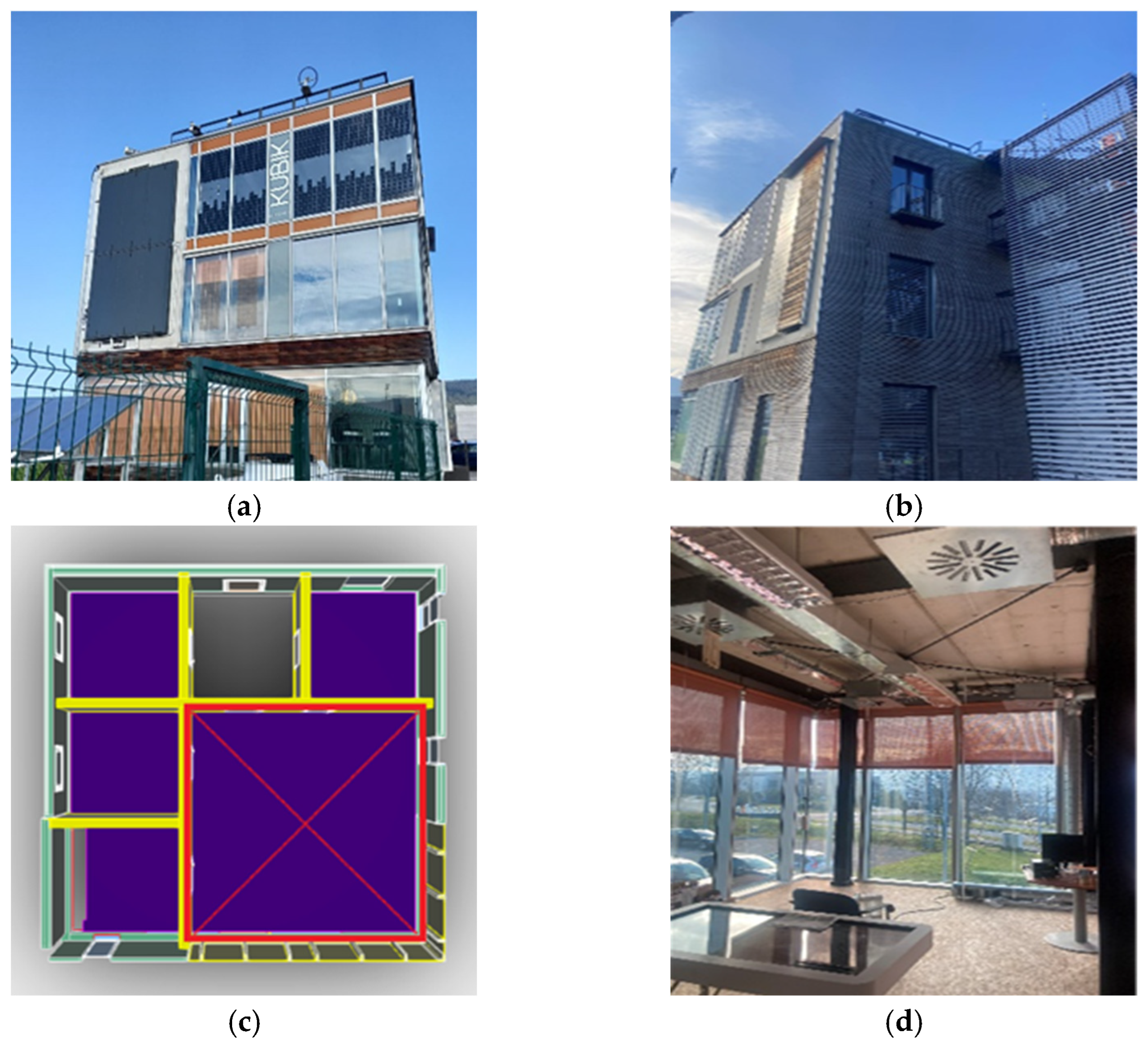
For these experimental tests, a room in the KUBIK experimental building, setup by Tecnalia (see Figure 1), was used. Various tests were carried out to compare different ventilation conditions. Those tests were conducted during the night to avoid solar radiation effects. Test 1 was performed from 12 June 2023 at 22:00 to 13 June 2023 at 8:00, and Test 2 from 15 June 2023 at 22:00 to 16 June 2023 at 8:00.

For both experiments, CFD validation was performed under steady-state conditions using the final 30 min of measurements, when CO₂ concentrations and airflow rates were observed to be quasi-stationary. A steady-state formulation was intentionally adopted as a conservative, near worst-case representation for regulatory compliance assessment, as it approximates sustained occupancy and constant emission and ventilation rates. For Test 2 (15 June 2023 at 22:00 to 16 June 2023 at 08:00), the last 30 min were likewise used for model validation. This assumption may overestimate exposure relative to real classrooms, where occupancy and ventilation typically vary over time.

The sampling system at the KUBIK experimental building is “continuous sampling”. In these tests, a continuous sweep is made over the communications bus and the sensors respond. The effective sampling frequency was below 1 min, although logging occurred only when variable changes were detected.

The ventilation system airflow rate was continuously monitored, and specific measures were implemented to minimize uncontrolled air infiltrations within the room. The space was properly sealed for experimental purposes, including keeping the door fully closed and ensuring the absence of external openings such as windows. These precautions allowed the airflow supplied by the mechanical ventilation system to be considered representative of the indoor air exchange, thereby enabling a reliable assessment of ventilation performance and CO₂ distribution for indoor air quality analysis.

The room has, on the one hand, a distribution system of the CO₂ pollutant and, on the other, a system for measuring its concentrations. The room is also equipped with a ventilation system through which the renewed air enters and allows the polluted air to be evacuated. The ventilation system is made up of the air supply system and the air exhaust system. The air supply system injects new air into the room, while the air exhaust system removes the polluted air. As for the air supply configuration, there are two supply arrangements in this room, one at ceiling height, and another at floor height. All of these elements are specified in the next sections.

2.1. CO₂ Controlled Injection Network

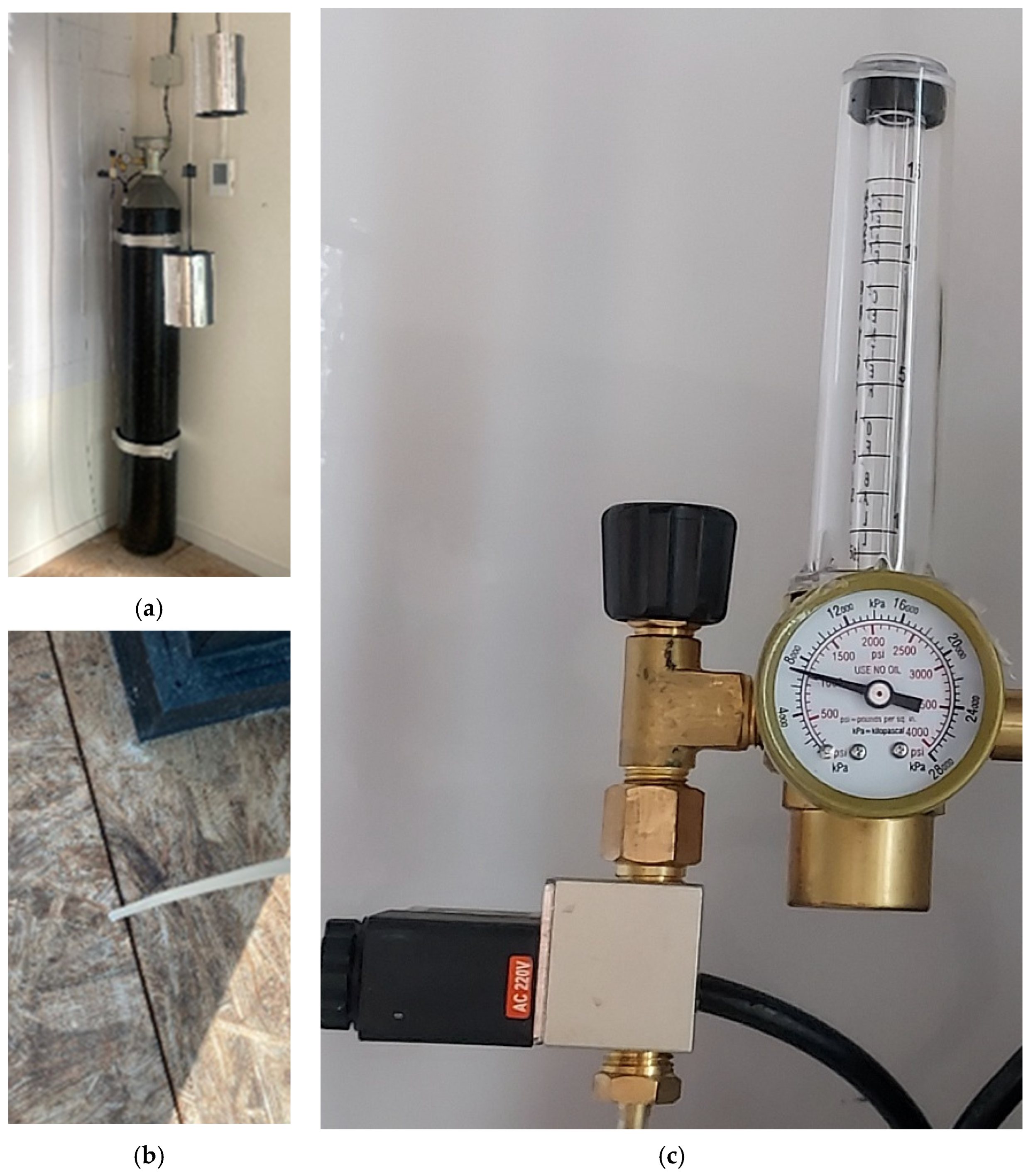
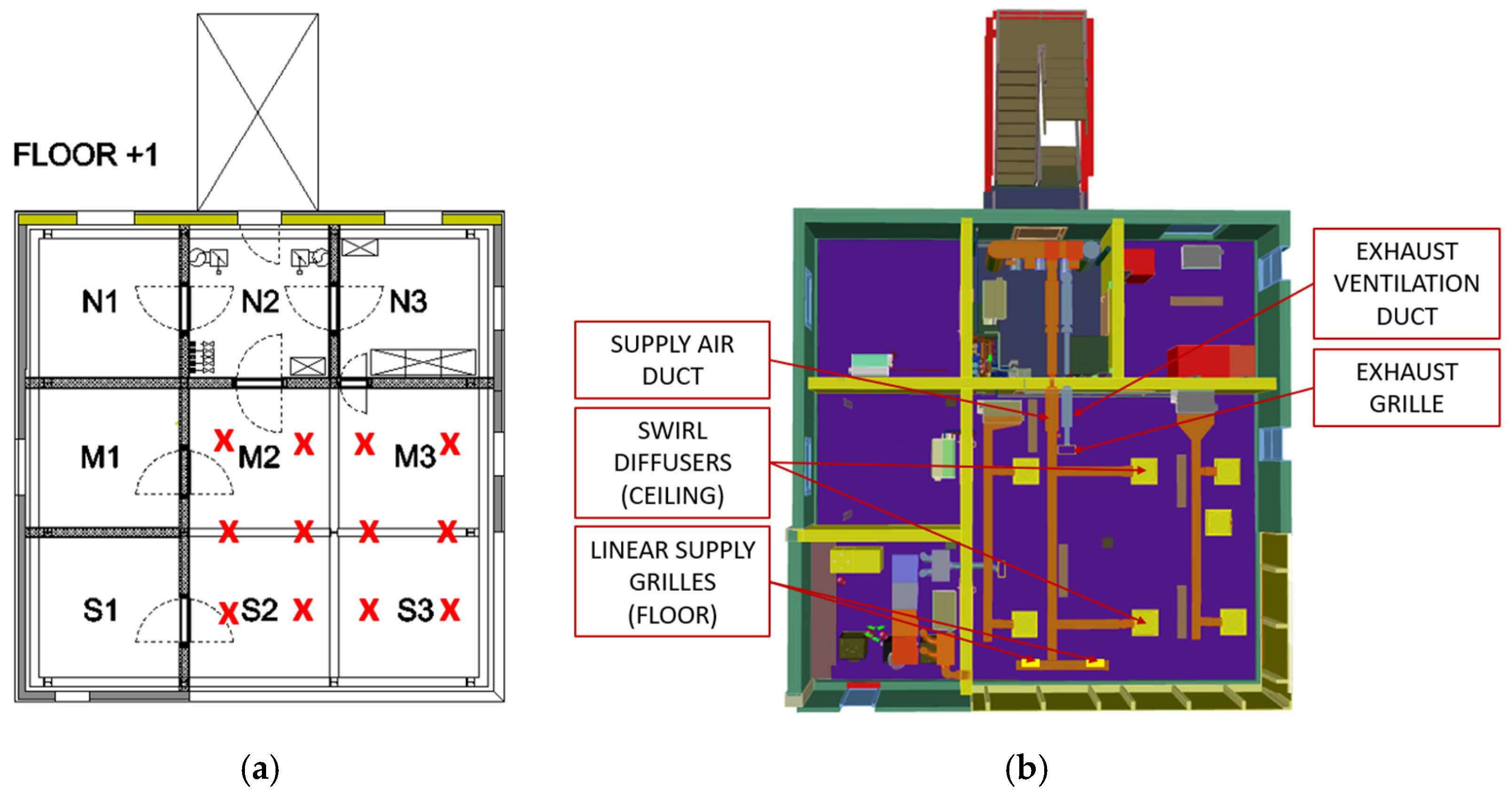
The CO₂ injection network consisted of a pressurized CO₂ cylinder equipped with a control valve to regulate the injection rate. The gas was distributed within the room through a set of 6 mm diameter release tubes (Figure 2), strategically arranged to emulate multiple emission points. CO₂ was discharged at floor level, and the injection flow rate was kept constant throughout all experiments. Floor-level release represents a conservative condition with respect to stratification and local accumulation, thereby enabling a cautious assessment of ventilation effectiveness within the occupied zone. The locations of the release tubes are indicated by red crosses in the plan view shown in Figure 3a.

It should be mentioned that injecting CO₂ at floor level ignores the body heat of real students. These upward thermal plumes may influence floor-level airflow dynamics. In the experimental room design stage, it was decided to locate the CO₂ injection at floor level, as technically it is simpler for modifying the distribution of ‘dummy occupants’ within the experimental space.

2.2. Air Supply System

There are two different types of air supply systems; Figure 3b shows their arrangement:

-

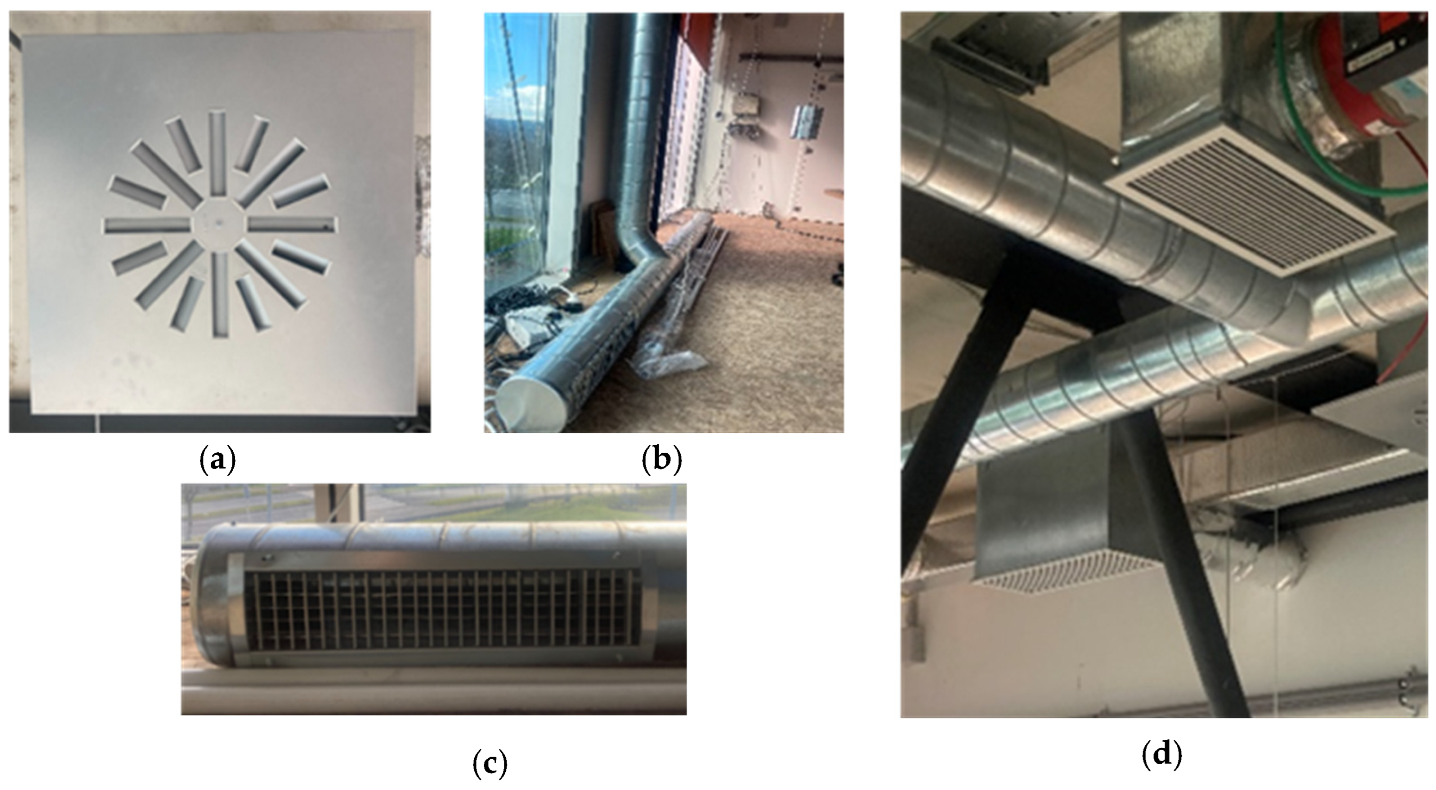
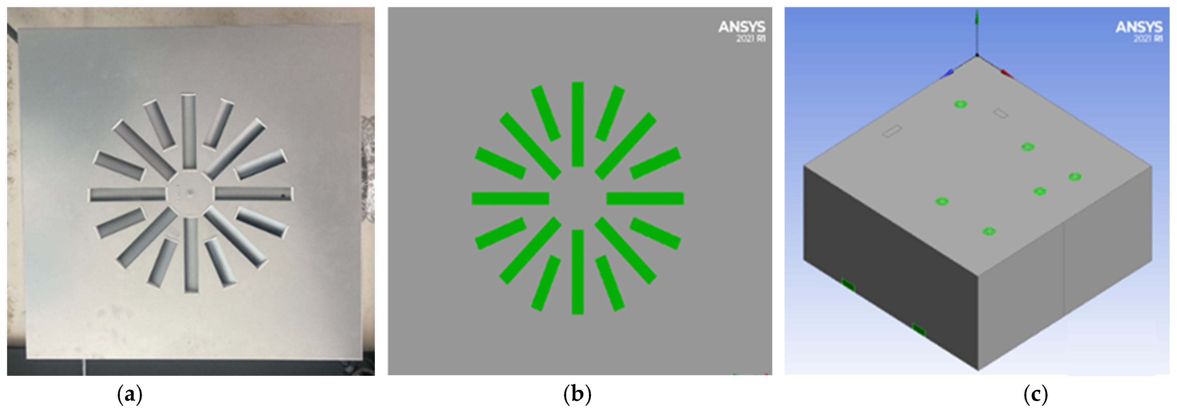
First, the ceiling ventilation system. The ceiling air supply system has 2 diffusers to emit clean air into the room. These fans are formed by a useful area divided into rectangles of two different sizes. In addition, all of these sections have an inclination of 45°, which causes the air to come out with a rotational movement. See Figure 4a.

-

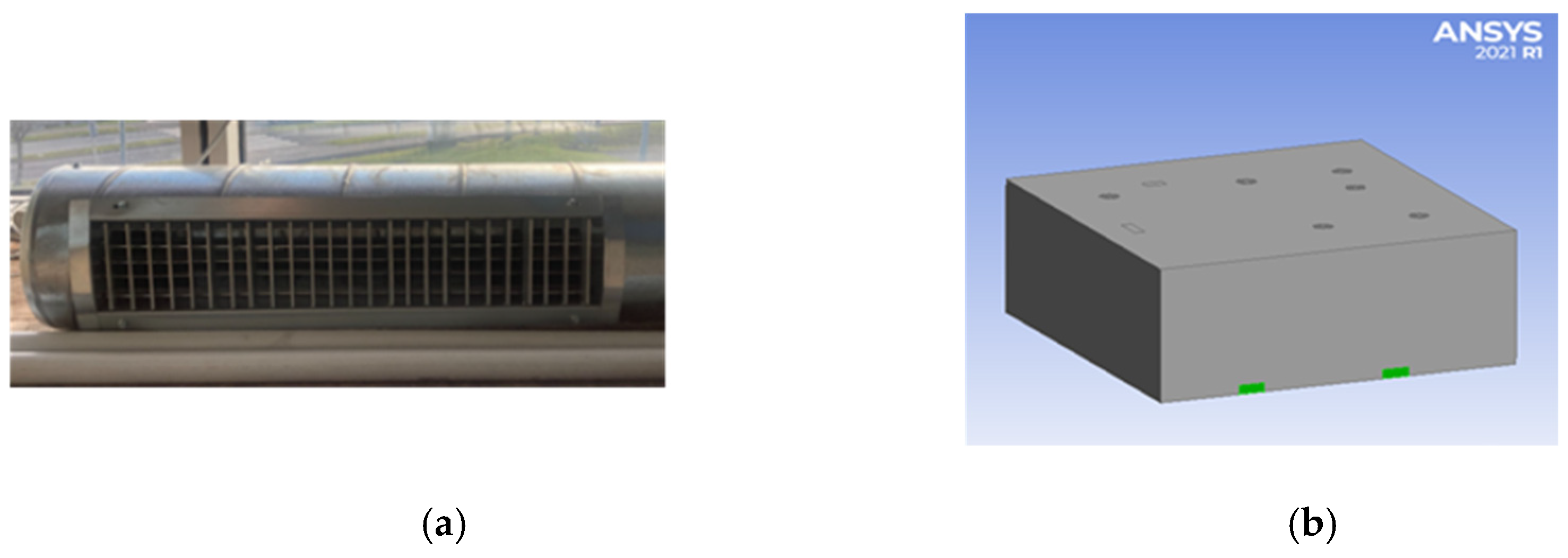
Second, the floor ventilation system. This system is equipped with 2 linear supply grids that emit clean air. The geometry of these grids causes the air to be expelled perpendicularly to the surface of these. (See Figure 4b).

A specific Monitoring Control Unit (MCU) is available to control the air inlet flow in the test space and thus the ventilation in the test cells. The airflow rate supplied by each ventilation configuration was recorded continuously and later used as CFD boundary conditions.

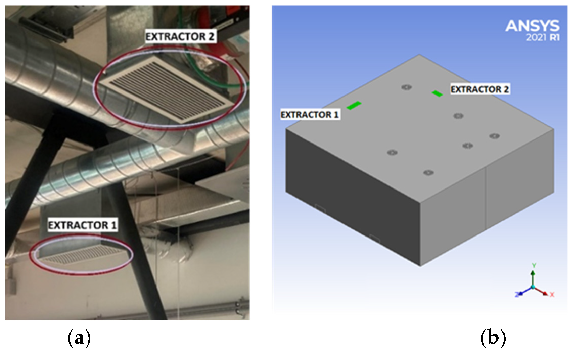
Figure 4. Ventilation system components: (a) Ceiling-mounted air supply diffusers with inclined vanes inducing rotational airflow, (b,c) floor-level linear supply grilles providing perpendicular air injection, and (d) mechanical exhaust outlet used for air extraction.

Figure 4. Ventilation system components: (a) Ceiling-mounted air supply diffusers with inclined vanes inducing rotational airflow, (b,c) floor-level linear supply grilles providing perpendicular air injection, and (d) mechanical exhaust outlet used for air extraction.

2.3. Air Exhaust System

For the extraction of polluted air, and to ensure the renewal of indoor air, it is necessary to have an exhaust method. Two exhaust fans are installed, although only one was used in these tests, the one belonging to the primary ventilation system, see Figure 4a–d.

2.4. Measuring System

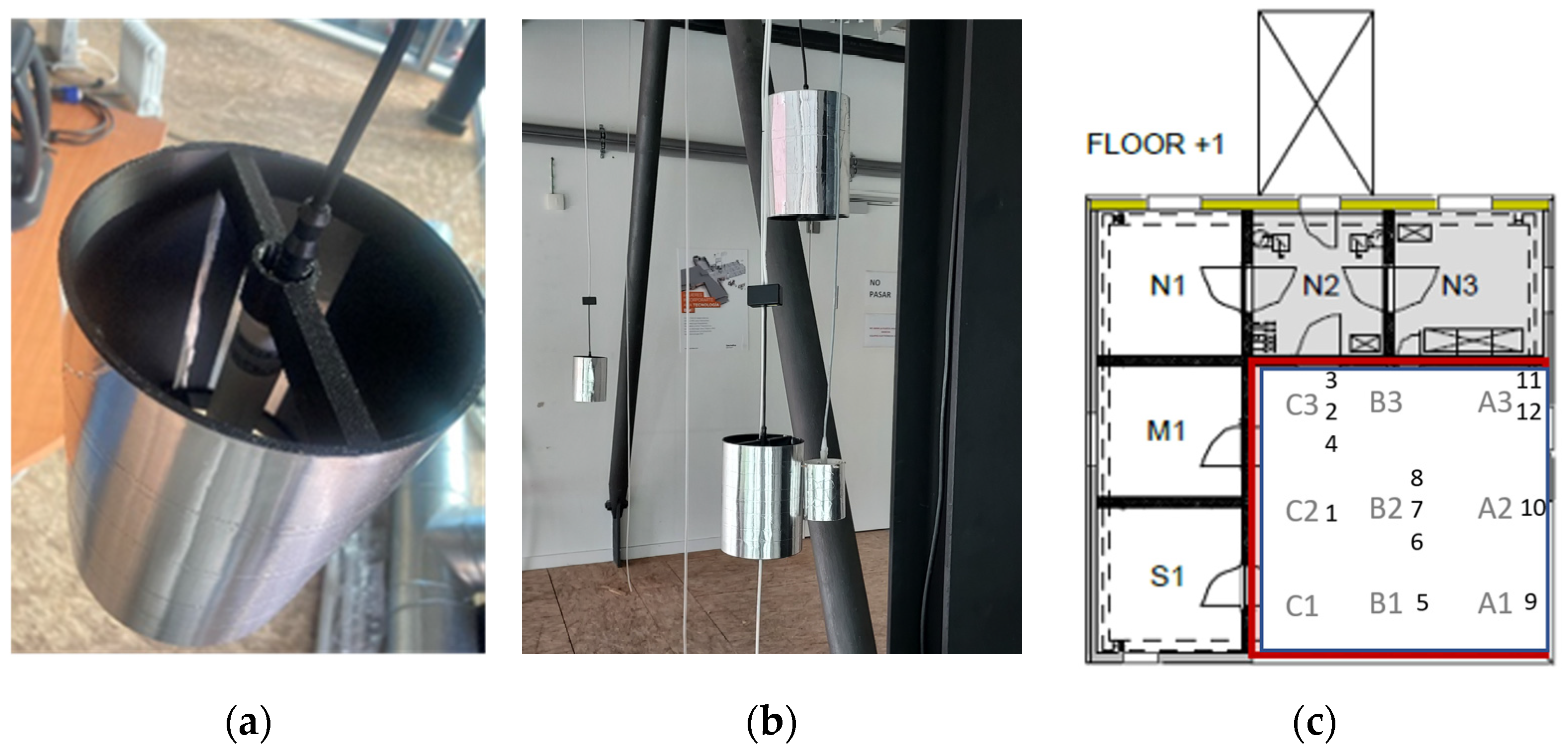
The system has 12 probes, see Figure 5, of equal characteristics, with a CO₂ measuring range of [0–5000] ppm and an accuracy of 50 ppm + 3% of the measured value. Used CO₂ sensors are the E + E brand, model EE872-M. All sensors were factory-calibrated and verified prior to the experiments. The CO₂ sensors are listed from 1 to 12, respectively, and located as shown in Figure 5c and

Table 1. Spatial coordinates and vertical position of CO₂ sensors installed in the experimental room, indicating measurement locations used for CFD validation.

N° Sensor	Cell Position	Height (cm)
1	C2	110
2	C3	110
3	C3	170
4	C3	10
5	B1	110
6	B2	20
7	B2	110
8	B2	170
9	A1	110
10	A2	110
11	A3	170
12	A3	110

. The sensors are located at different heights, as described in Table 1.

3. Computational Setup

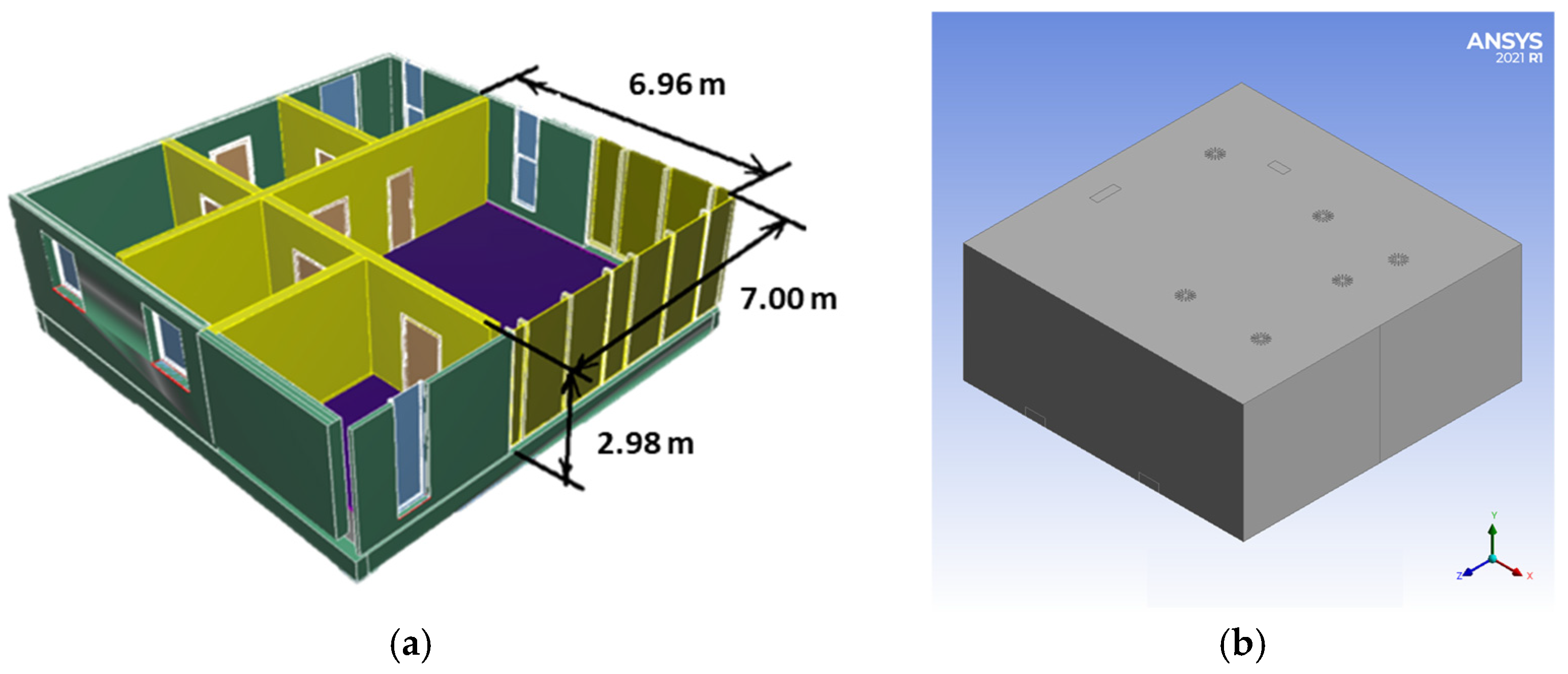
The CFD code ANSYS Fluent, release 2021R1, was used [36]. Three-dimensional steady-state RANS modelling was performed. Considering the test room dimensions, the computational domain covers the entire room. Figure 6 shows the room dimensions and the computational domain.

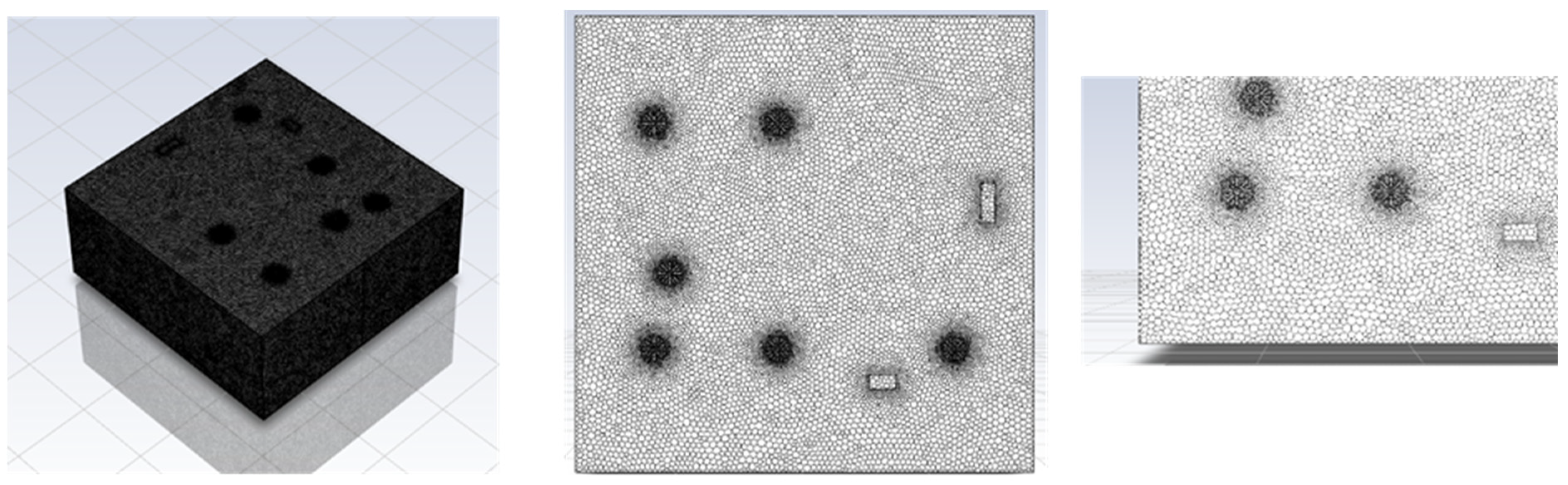
The computational grid used in this work is the polyhedron mesh (Figure 7) due to its advantages for reducing the computational time up to 50%. Mesh size is selected after performing a mesh sensitivity analysis. The fluid flow pattern through the room when the ventilation system is working was modelled for the mesh analysis. The results of three mesh sizes were compared: a fine mesh with 772,215 elements (MESH 1), a medium size mesh with 531,975 elements (MESH 2), and a coarse mesh with 345,732 elements (MESH 3). The grid convergence index (GCI) method [37,38], which is based on the Richardson extrapolation, was used for the mesh sensitivity analysis. Accepted GCI values for a good mesh quality must be below 5%, and they are very good if they are below 2%. The results obtained in this work are 2.50% in MESH 2 and 1.99% in MESH 1. Therefore, both meshes are of good quality for simulations. In this work, MESH 2 was chosen, as the computational cost is lower [39]. It has been concluded that the defined grid provides both good accuracy and consistency in the results on the one hand and an acceptable CPU time on the other.

The numerical simulation was performed using a pressure-based steady-state solver. Spatial discretization for governing equations, including momentum and CO₂ transport, was managed via second-order upwind schemes to maintain numerical accuracy. Convergence was achieved when the monitoring residuals dropped below 10⁻⁴ for flow dynamics and 10⁻⁶ for the species transport equation.

The models used during the modelling are the species transport model, which allows both components (air and CO₂) to be considered while calculating the diffusion between them and their concentrations at all points, and the SST k-ω model, which is well suited at high and low Reynolds numbers [36]. The SST k-ω model was selected due to its capability to accurately resolve near-wall flows and recirculation zones, which are critical in indoor airflow simulations involving low Reynolds numbers.

The boundary conditions were defined directly from the experimental setup. Therefore, although the specific numerical values differ for each test (as detailed in Section 4), the type of boundary condition applied remained the same in all simulations.

Table 2. Boundary conditions applied in the CFD simulations, including inlet airflow rates, CO₂ injection rates, and outlet pressure conditions based on the experimental setup.

	Ventilation Air	CO2 Injection	Air and/or CO2 Outlet
Boundary condition type	Velocity inlet	Mass flow inlet	Pressure outlet

summarizes the boundary conditions used in each case, including the ventilation airflow rates and the CO₂ injection mass flow imposed as inputs to the CFD model.

The room and ventilation system domains are modelled in CFD, as shown in Figure 8, Figure 9 and Figure 10.

4. Results

The goal of this work is to analyze educational classrooms located in Spain and whether the ventilation flow rates and occupancy density defined by the RTIB’s indirect method and TBC regulations [32,33] are sufficient to comply with the emission limits defined by the RTIB’s direct method.

For this purpose, a simplified yet computationally efficient 3D CFD model was developed and validated to predict airflow patterns and CO₂ distribution in an indoor space. To do this, experiments were first carried out in the KUBIK experimental room, and they were later modelled by CFD (Section 4.1). Once validated, the model was applied to analyze the ventilation flow rates and occupancy density defined by the RTIB and TBC regulations (Section 4.2). For the regulatory scenarios, CFD results were compared with the CO₂ concentration build-up calculator tool [40], which provides spatially averaged concentration estimates. All analyses were conducted under steady-state conditions.

4.1. Three-Dimensional CFD Model Validation

In this section, the model was validated by comparing the CO₂ concentrations measured by the experimental test and the CFD modelling results. Two experimental tests were carried out: 4.1.1 CO₂ distribution analysis by a ceiling-type ventilation, and 4.1.2 CO₂ distribution analyzed by a floor-type ventilation system. During the experiments, data on airflow rates, CO₂ distribution, and inlet temperatures were all recorded. Validation was performed under steady-state conditions.

Arithmetic Mean Error (Equation (1)) and Mean Bias Error (MBE) (Equation (2)) were used to quantify the relative error at each sensor location by comparing the experimentally measured CO₂ concentration in the KUBIK test room with the corresponding CFD prediction.

$$\mathrm{A}\mathrm{r}\mathrm{i}\mathrm{t}\mathrm{h}\mathrm{m}\mathrm{e}\mathrm{t}\mathrm{i}\mathrm{c}\text{\_}\mathrm{e}\mathrm{r}\mathrm{r}\mathrm{o}\mathrm{r}\text{\_}\mathrm{i}(\%)=\left(\right(\mathrm{C}\text{\_}\mathrm{e}\mathrm{x}\mathrm{p},\mathrm{i}-\mathrm{C}\text{\_}\mathrm{C}\mathrm{F}\mathrm{D},\mathrm{i})/\mathrm{C}\text{\_}\mathrm{e}\mathrm{x}\mathrm{p},\mathrm{i})\times 100$$

(1)

where

-

Arithmetic_error_i (%) is the relative error at sensor i (in %);

-

C_exp, i. is the experimentally measured CO₂ concentration at sensor i (ppm);

-

C_CFD, i. is the CO₂ concentration predicted by the CFD model at the same sensor location i (ppm);

-

i = 1,…, N, with N being the total number of sensors.

$$\mathrm{M}\mathrm{B}\mathrm{E}\left(\%\right)={\displaystyle \frac{1}{\mathrm{N}}}{\displaystyle \sum _{i=1}^N}(C_{CFD,i}-C_{exp,i})\times 100$$

(2)

where

-

$C_{exp,i}$ is the experimentally measured CO₂ concentration at sensor i (ppm);

-

$C_{CFD,i}$ is the CO₂ concentration predicted by the CFD model at the same sensor location i (ppm);

-

i = 1,…, N, with N being the total number of sensors.

4.1.1. TEST 1: Ceiling Ventilation and CO₂ Diffusion

In this experiment, the ceiling ventilation system and the injection of the contaminant were kept in operation. The aim was to observe the effect of this type of ventilation on the diffusion of the contaminant. The airflow through the ventilation considered was 386.75 m³/h, while the pollutant flow was 0.0283 m³/h. The air entering through the ventilation system was considered to have the same concentration of CO₂ as the outside environment, i.e., 410 ppm of CO₂. The air entered with a temperature of 26.05 °C. All these data were taken from the experimental measurements.

The results obtained in the experimental room and the CFD model under these conditions are shown in

Table 3. Comparison of CO₂ concentrations (ppm) obtained from CFD simulations and experimental measurements for Test 1 (ceiling ventilation), including relative error at each sensor location.

Sensor	[CO2] (ppm) CFD Model	[CO2] (ppm) Exp. Room	Arithmetic Mean Error (%)	MBE (%)
sensor 1	472.05	571.67	17%	-
sensor 2	469.07	558.33	16%	-
sensor 3	466.54	596.50	22%	-
sensor 4	462.48	645.75	28%	-
sensor 5	503.05	572.25	12%	-
sensor 6	464.13	556.75	17%	-
sensor 7	477.77	539.00	11%	-
sensor 8	480.71	537.00	10%	-
sensor 9	467.16	596.00	22%	-
sensor 10	471.62	586.50	20%	-
sensor 11	478.11	663.33	28%	-
sensor 12	473.46	771.00	39%	-
Total			20%	−125 ppm

Note: Errors are calculated according to Equation (1).

:

Comparing the results of the modelling and the experimental results in Table 3, the CFD model gives lower values than the experimental data. The total error calculated is 20%, which could be caused by the objects that were in the real room (such as columns, a table, and a chair) but were not considered in the modelling. It should be mentioned that the most notorious errors occur in sensors 4, 11, and 12, specifically, when experimental concentrations are higher. These results indicate an acceptable agreement between experimental and numerical data. Errors are consistent with previous indoor airflow CFD validation studies reporting discrepancies between 10 and 25% under simplified geometries. The MBE provides an error of −125 ppm. This means that the CFD model is underestimating the CO₂ prediction.

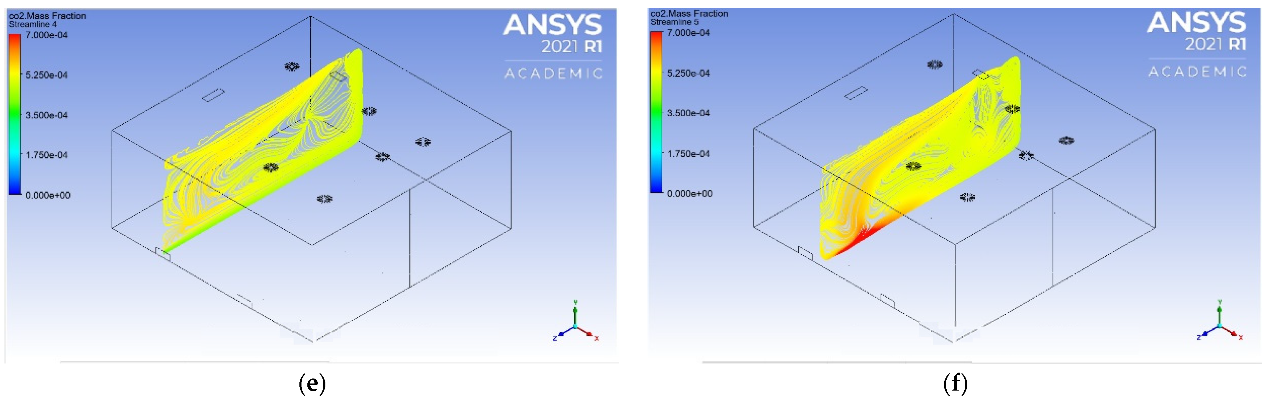
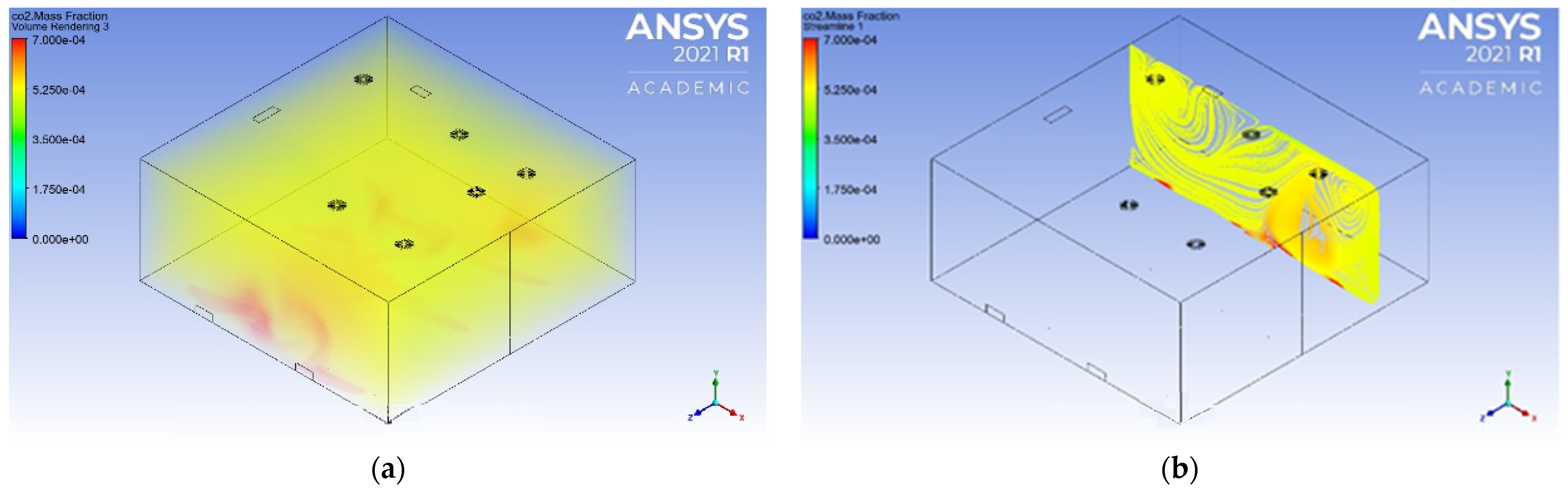
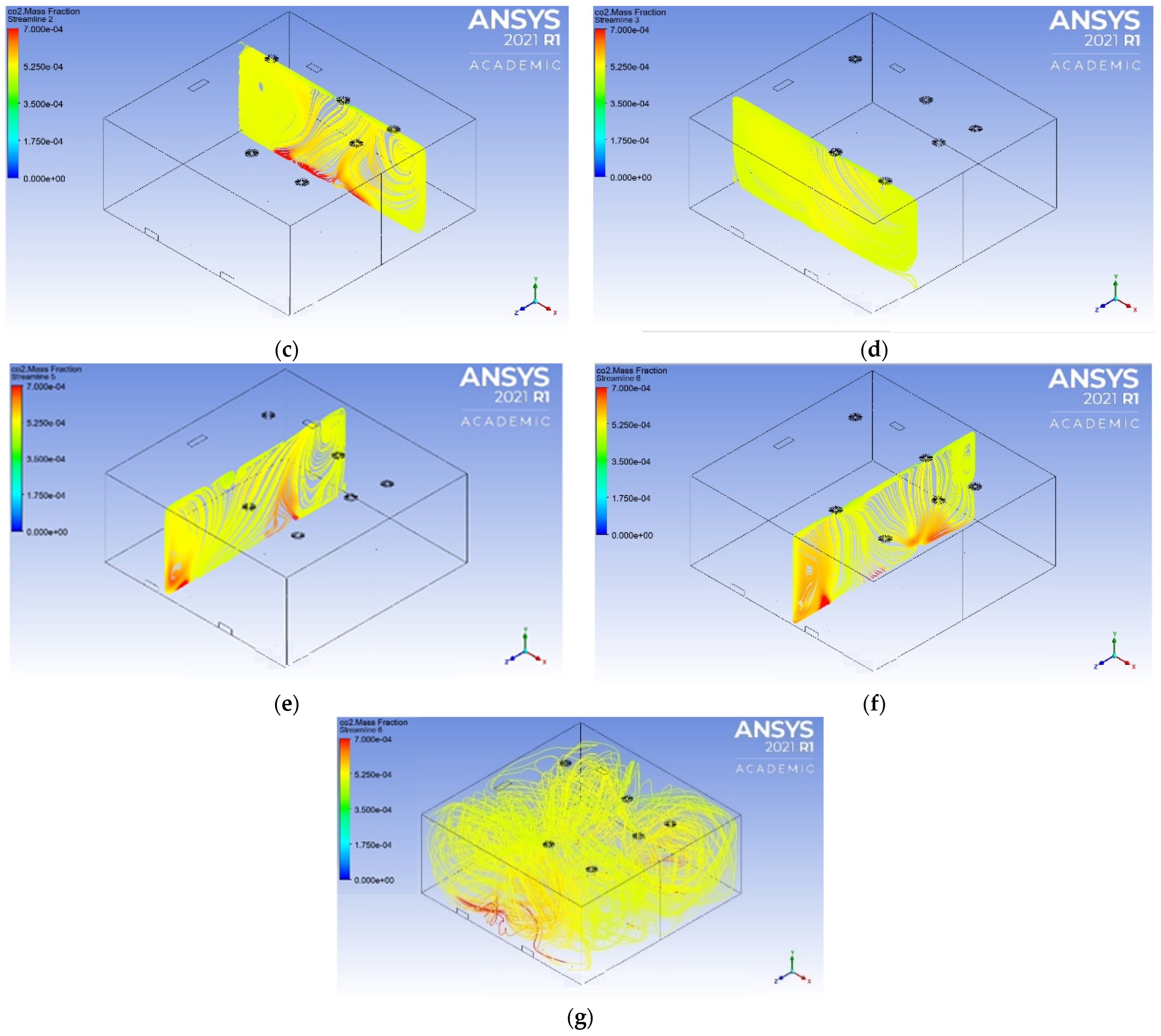
Analyzing Figure 11, the CO₂ concentration is higher near the floor level, decreasing with the height. The spatial distribution highlights non-uniform concentration patterns within the room.

4.1.2. TEST 2: Floor Ventilation and CO₂ Diffusion

The second model validation campaign simulates the behaviour of the contaminant in the case of floor ventilation. The injected airflow rate was 387 m³/h (with a concentration of 410 ppm of CO₂), while the contaminant flow rate was 0.0283 m³/h. The flow injection temperature, in this case, was 24.92 °C. All these data were taken from the experimental measurements.

The results obtained in the experimental room and the CFD model under these conditions are shown in

Table 4. Comparison of CO₂ concentrations (ppm) obtained from CFD simulations and experimental measurements for Test 2 (floor ventilation), including relative error at each sensor location.

Sensor	[CO2] (ppm) CFD Model	[CO2] (ppm) Exp. Room	Arithmetic Mean Error (%)	MBE (%)
sensor 1	460.92	534.33	14%	-
sensor 2	459.25	542.33	15%	-
sensor 3	463.92	586.33	21%	-
sensor 4	522.77	645.75	19%	-
sensor 5	500.78	556.33	10%	-
sensor 6	489.09	562.00	13%	-
sensor 7	468.80	521.00	10%	-
sensor 8	478.86	529.33	10%	-
sensor 9	541.37	587.50	8%	-
sensor 10	492.53	591.67	17%	-
sensor 11	472.62	553.00	15%	-
sensor 12	473.85	602.00	21%	-
Total			14%	−82 ppm

Note: Errors are calculated according to Equation (1).

:

In this test, the CFD model again gives lower values than the experimental data. The total error is 14%, which is lower than in Test 1. This confirms the consistency of the CFD model under different ventilation configurations. The MBE provides an error of −82 ppm. This means that the CFD model is underestimating the CO₂ prediction.

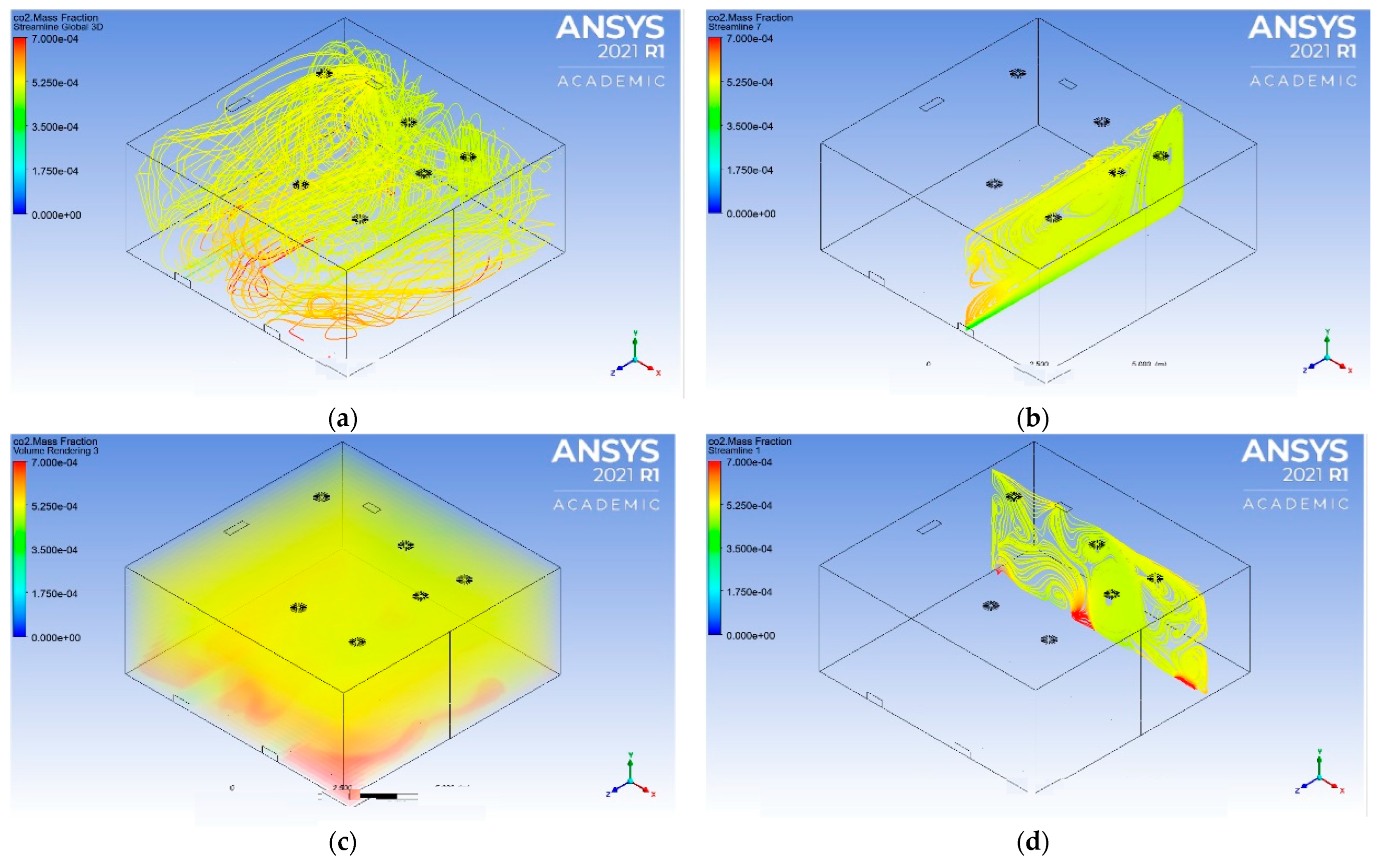
The contaminant distribution shows that, in Figure 12, it is possible to see that the point of greatest concentration is still at floor level. Even so, the air injection at the height of the floor results in lower CO₂ levels.

4.2. Regulation Flow Rates and Occupancy Density Analysis to Comply with Emissions Limits

The ventilation flow rates and occupancy densities applied in this study are defined according to the Spanish regulatory framework, specifically the RTIB and the Technical Building Code (TBC).

Table 5. Indoor air quality (IAQ) categories and corresponding ventilation requirements defined by the Spanish Regulation for Thermal Installations in Buildings (RTIB) [32], including external airflow rates and allowable indoor CO₂ concentration increases relative to outdoor levels.

Category	Use	IAQ Level	External Airflow Rate (L/s Per Person)	Maximum CO2 Increase (ppm)
IDA1	Hospitals, nursery school	High	20	350
IDA2	Offices, classrooms	Medium–high	12.5	500
IDA3	Restaurants, hotels, theatre	Medium	8	800
IDA4	Other uses	Low	5	1200

summarizes the indoor air quality categories and corresponding ventilation requirements, while

Table 6. Occupancy density values defined in the Spanish Technical Building Code (TBC, DB-SI) [32,33] for educational buildings, expressed as usable floor area per occupant.

Space Type	Occupancy Density (m2/Person)
General building areas	10
Laboratories, workshops, gyms, drawing rooms	5
Classrooms (except nursery)	1.5
Nursery/Preschool classrooms and library reading rooms	2

presents the occupancy density values used for educational spaces.

Once the model had been validated, the ventilation flow rates and occupancy density defined by the RTIB’s and TBC’s regulations (Table 5 and Table 6) for educational classrooms located in Spain were analyzed. The objective was to evaluate whether the ventilation rates defined by the RTIB indirect method comply with the CO₂ limits established by the direct method. Therefore, the simulations were carried out considering the KUBIK building’s experimental room as an educational classroom located in Spain. For the analysis, the occupancy density and removed airflow rates criteria, as defined by DB SI of the TBC [33] and RTIB standards [32], were followed to ensure a good IAQ.

The experimental room has an area of 36 m², which, considering Table 5 and Table 6 for a teaching classroom (the most critical case), 36 m² is equivalent to an occupation of 24 people, which supposes an occupancy of 1.5 m²/person. Considering a metabolic rate of 1.2 met and the occupancy of 24 people, the equivalent CO₂ contribution for this situation is 0.12096 L/s. The air inlet flow rates in the room are equivalent to those that the RTIB’s indirect method standard awards for this type of space; basically, a type IDA 2 space with a flow of 12.5 L/s per person [32]. Considering the occupation of 24 people and the minimum flow per person, it can be concluded that it is necessary to inject 1080 m³/h of clean air through the ventilation system. It was assumed that the air entering the room comes directly from outside, so this inlet air has the same concentration of CO₂ as the outside air, i.e., 410 ppm of CO₂.

With the 3D model validated in Section 4.1, the CO₂ distribution for this hypothetical situation was analyzed for both ventilation systems, ceiling and floor. There were no experimental data for the defined situation, but the results were compared with the known CO₂ concentration build-up calculator [40]. As in the previous sections, for the calculation of the error between the CFD model and the CO₂ level build-up calculator [40], Equation (1) was used.

4.2.1. TEST 3: Ceiling Ventilation and CO₂ Diffusion Following RTIB Standard

In this test, the diffusion of the CO₂ pollutant was modelled when the ventilation system injects new air from the height of the ceiling. Therefore, for occupation by 24 people, the air entering the room is 1080 m³/h, with 410 ppm of CO₂, and the generation of CO₂ of 0.12096 L/s. The CO₂ injection was modelled at the height of the ground, as in the experimental test, whose values were used previously to validate the CFD model.

Table 7. Comparison of CO₂ concentrations (ppm) predicted by CFD simulations and the CO₂ build-up calculator for Test 3 (ceiling ventilation under RTIB ventilation rates and TBC occupancy), including relative error.

Sensor	[CO2] (ppm) CFD Model	[CO2] (ppm) CO2 Concentration Build-Up Calculator [40]	Error (%)
sensor 1	1270.62	1010	−25%
sensor 2	1216.46	1010	−20%
sensor 3	1232.38	1010	−21%
sensor 4	1202.34	1010	−18%
sensor 5	1542.64	1010	−51%
sensor 6	1284.26	1010	−26%
sensor 7	1617.33	1010	−58%
sensor 8	1448.14	1010	−42%
sensor 9	1126.98	1010	−11%
sensor 10	1272.83	1010	−25%
sensor 11	1392.37	1010	−36%
sensor 12	1363.86	1010	−34%
Total	26%

Note: Errors are calculated according to Equation (1).

shows the CO₂ concentrations at the different points where the sensors are placed. The errors obtained between the tool and the CFD model are also shown.

It is possible to see that the values provided by the CO₂ level build-up calculator [40] are lower than those obtained by the CFD model. Both approaches predict CO₂ concentrations exceeding 910 ppm. In addition, the tool does not consider the location of the air supply system and its effect, for example, where the concentration is higher due to the approximation to the CO₂ distribution system.

Additionally, in both cases, the CO₂ concentration values are greater than the maximum CO₂ distribution permitted by the RTIB’s direct method, i.e., 910 ppm. It can be concluded that the airflow rate values, as defined by the RTIB’s indirect method in combination with the TBC-defined occupancy density, do not guarantee CO₂ concentration values lower than those defined by the RTIB’s direct method, i.e., 910 ppm [32].

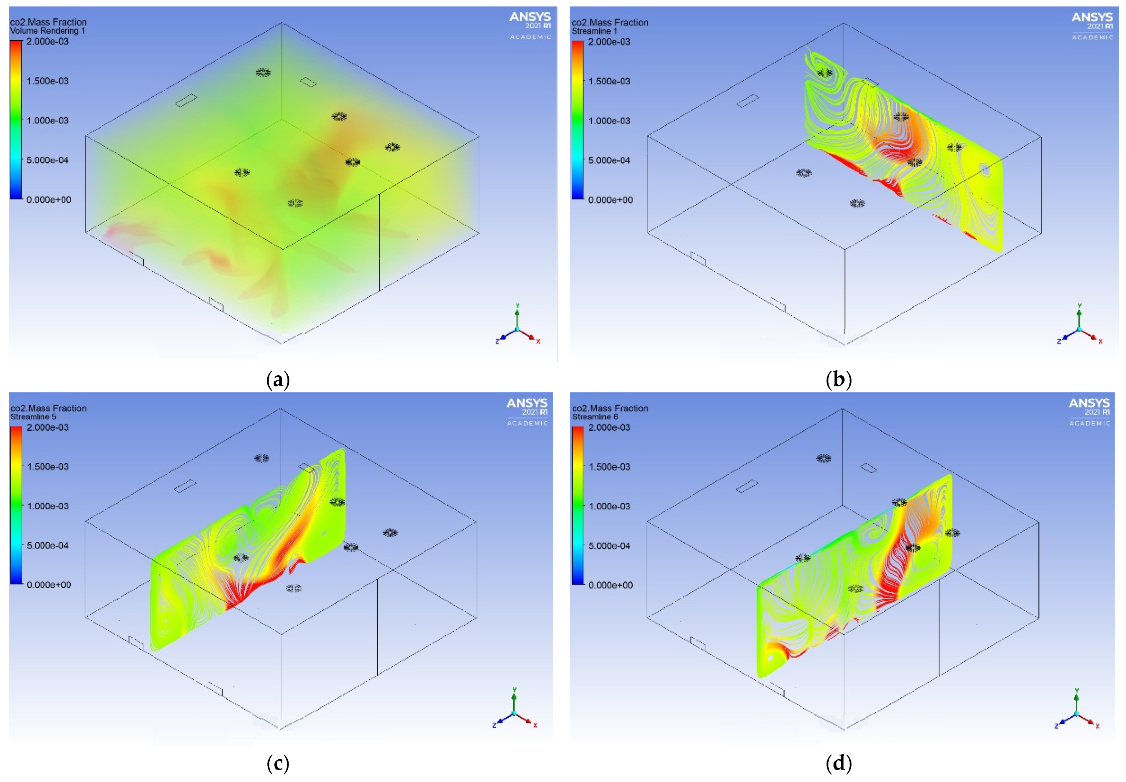
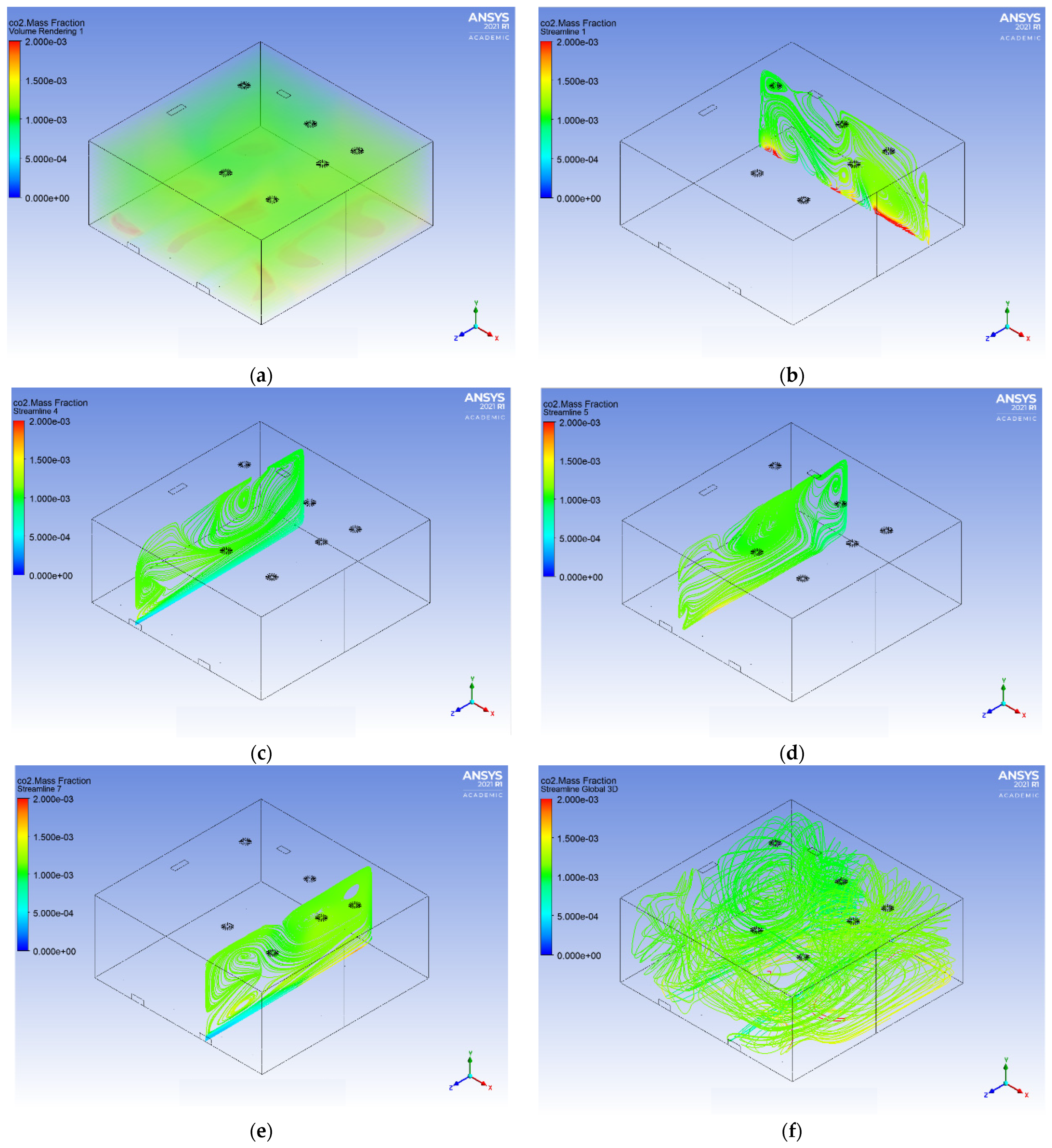
Figure 13 shows that the distribution of CO₂ is quite similar to the one in Test 1, with the highest concentrations being at floor level. From this it can be deduced that, when the locations of the inputs and outputs are the same, the areas with the highest concentration of CO₂ will remain the same despite changing the flows. As for the CO₂ values obtained, the concentrations are higher than the limits established by the RTIB [32]. For this reason, it is concluded that, with the ventilation flow rates defined by the indirect method and the occupancy density defined by the TBC and current fan location, the CO₂ ppm limits defined in the RTIB’s direct method are exceeded.

4.2.2. TEST 4: Floor Ventilation and CO₂ Diffusion Following the RTIB Standard

This new test models the behaviour of CO₂ in the test room of the KUBIK building when it is occupied by 24 people, with the ventilation system at floor level. The amount of renewed air that must enter through the ventilation system, according to the RTIB’s indirect method, is 1080 m³/h (with 410 ppm of CO₂). The CO₂ generation equivalent to the 24 people is still 0.12096 L/s and is injected at floor level through the distribution system.

Table 8. Comparison of CO₂ concentrations (ppm) predicted by CFD simulations and the CO₂ build-up calculator for Test 4 (floor ventilation under RTIB ventilation rates and TBC occupancy), including relative error.

Sensor	[CO2] (ppm) CFD Model	[CO2] (ppm)CO2 Concentration Build-Up Calculator [40]	Error (%)
sensor 1	1099.77	1010	−9%
sensor 2	1023.94	1010	−1%
sensor 3	1104.75	1010	−9%
sensor 4	1858.33	1010	−81%
sensor 5	1060.35	1010	−5%
sensor 6	1088.57	1010	−7%
sensor 7	1024.60	1010	−1%
sensor 8	1029.23	1010	−2%
sensor 9	1611.46	1010	−57%
sensor 10	1516.34	1010	−48%
sensor 11	1556.11	1010	−52%
sensor 12	1641.29	1010	−60%
Total	−9%

Note: Errors are calculated according to Equation (1).

shows the CO₂ concentrations at the different points where the sensors are placed. The errors obtained between the tool and the CFD model are also shown.

For both tests in these hypothetical conditions (Tests 3 and 4), the CO₂ injection and airflow entering the room are the same; the difference between them is the mechanical ventilation type and its location. The CO₂ calculator tool gives the same results for both tests despite the differences in the ventilation system. However, CFD results show spatial variations in concentration depending on the ventilation configuration. As concluded with the results from Tests 1 and 2, there is a more uniform air distribution with the floor ventilation system. The greatest variation is found in sensor 4, which is the sensor at a lower height. As mentioned above, the CO₂ injection is introduced at floor height, so it is logical that the concentrations of the gas will be higher near these points. This shows that, in addition to achieving logical values for the rest of the geometry, the CFD models have the advantage of being able to identify the most critical areas and observe the distribution of contaminants.

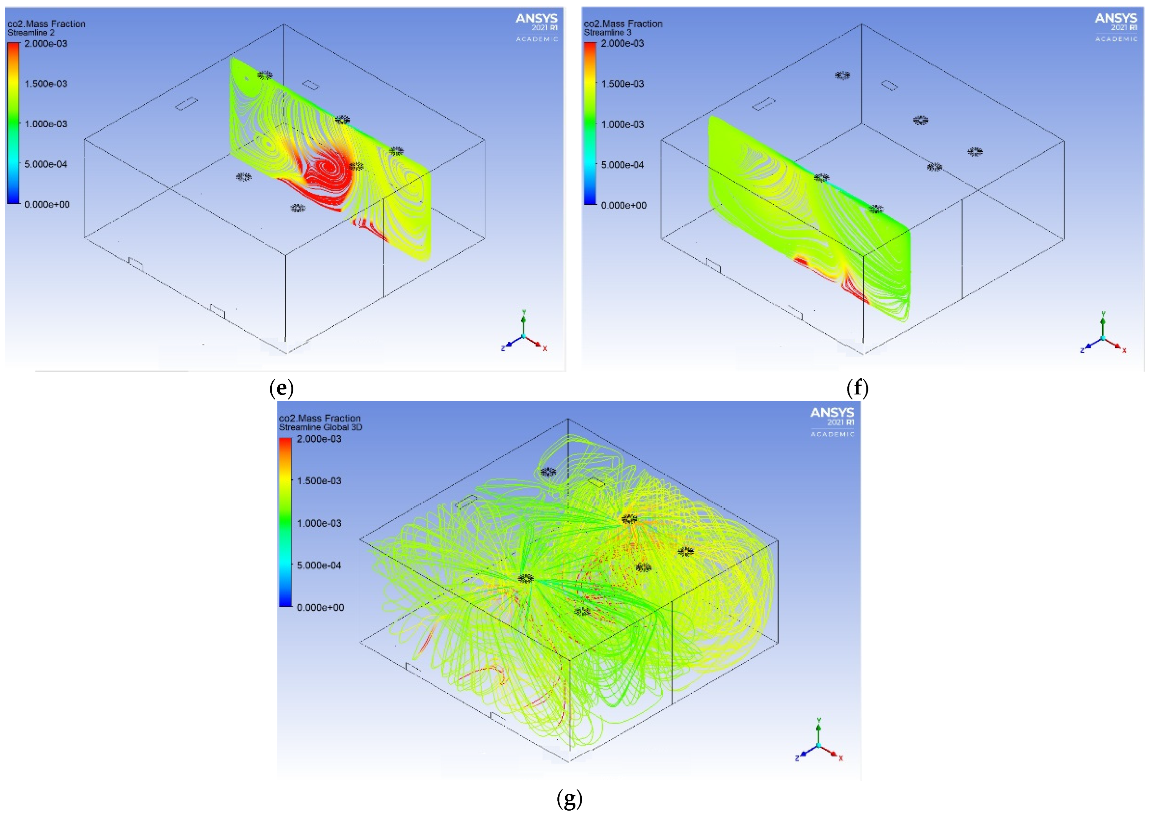
Figure 14 shows the distribution of the contaminant in the room.

As can be seen in Table 8 and Figure 14, the distribution of CO₂ is noticeably more homogeneous than in Test 3, with the most critical points being the CO₂ entry points. It is worth noting that the concentrations of CO₂ are also lower in this case. It can thus be concluded that floor ventilation provides better pollutant diffusion than ceiling ventilation. However, CO₂ concentrations still exceed the regulatory limit of 910 ppm [32].

Therefore, it can be concluded that, while the CO₂ concentration build-up calculator tool serves as an acceptable and computationally effortless method for early stage estimates of average indoor air quality, it remains fundamentally limited. Because it assumes a perfectly homogeneous fluid distribution, the tool is mathematically bound to underestimate localized concentration peaks. This highlights why 3D CFD modelling is necessary for practical engineering applications; unlike ideal zero-dimensional macro models, CFD provides the spatial resolution required to spot critical ventilation dead zones, short-circuiting paths, and localized air stagnation areas where CO₂ levels significantly exceed the room’s average.

5. Discussion

This work demonstrates that CFD models are a robust and suitable approach for indoor air quality assessment in educational environments. Thanks to the spatial resolution provided by the 3D CFD model, it is possible to assess which areas have the highest concentration of pollutants, i.e., the most critical areas. This implies that ventilation is not entirely effective in these areas, which helps to identify deficiencies in ventilation. These areas are directly associated with reduced ventilation effectiveness and would remain undetected using spatially averaged approaches. Furthermore, CFD modelling enables the evaluation of multiple scenarios with reduced experimental cost and time requirements.

First, the developed 3D CFD model was validated. The validation against experimental data obtained in the KUBIK facility shows average errors in the range of 14–20%, corresponding to an approximate reliability of 85%. In this way, the CFD model with a special geometry that saves computational time was validated. Additionally, some sources of error in the model validation may be due to uncertainties or calibration errors in the measuring material. In addition, the modelling results are compared with stationary measured experimental data. Although steady-state conditions were assumed, the experimental system is subject to small temporal fluctuations. On the other hand, minor air infiltrations through the envelope or door, even when closed, may influence the measured values. Finally, the use of a simplified geometry, excluding furniture elements such as columns, tables, and chairs, contributes to deviations, as these elements can promote the local accumulation of contaminants. Additionally, the CFD model tends to predict a more homogeneous CO₂ distribution than observed experimentally, particularly in zones with higher measured concentrations.

Second, the validated CFD model was used to analyze whether the ventilation flow rates defined by the RTIB’s indirect method in combination with the occupancy density defined by the TBC are sufficient to comply with the emission limits as defined by the RTIB’s direct method. CFD results were compared with the widely used CO₂ concentration build-up calculator tool [40]. Both approaches predict CO₂ concentrations exceeding the maximum limit established by the RTIB direct method (910 ppm). In educational settings, such systematic exceedances are particularly relevant, because elevated CO₂ is repeatedly associated with reduced attention and learning performance, making compliance not only a regulatory target but also a functional requirement for student well-being and productivity. Therefore, these results demonstrate that the RTIB indirect and direct methods are not equivalent, as the airflow rates prescribed by the indirect method are insufficient to meet the targets of the direct method. Based on the regulatory discrepancy exposed in this study, HVAC engineers sizing ventilation systems for high-occupancy educational spaces must prioritize the RTIB’s direct method (CO₂ concentration targets) over the prescriptive per-person flow rates of the indirect method to avoid compliance failures. To counteract the localized dead zones and stratification revealed by the CFD model, it is recommended to incorporate a volumetric airflow safety margin of 20% to 30% above regulatory minimums when utilizing standard ceiling mixing configurations. Alternatively, implementing floor-level ventilation systems represents a more efficient design path, as they optimize distribution homogeneity and lower overall CO₂ levels within the breathing zone without requiring excessive fan over-sizing.

CFD results were systematically higher than those obtained using the CO₂ concentration build-up calculator tool. This is because the CO₂ concentration build-up calculator tool considers an interior space with ideal conditions; specifically, a perfectly homogeneous distribution of air and CO₂ in the interior space. It also does not consider whether the ventilation is located in the floor or ceiling of the room. Therefore, this tool is suitable for preliminary estimations but may underestimate real exposure levels due to the assumption of ideal mixing conditions. These findings highlight a critical trade-off between indoor air quality and energy efficiency, which is central to sustainable building design.

Finally, the comparison between ceiling and floor ventilation systems reveals that the pollutant distribution is more homogeneous in the case of floor ventilation. In ceiling ventilation, the pollutant tends to accumulate in specific areas, where supply air does not reach. CO₂ accumulates near the floor level, with concentrations decreasing with height, indicating stratification. In contrast, floor ventilation promotes a more uniform airflow distribution and lower CO₂ concentrations. Therefore, under the analyzed conditions, floor-based ventilation systems provide more effective pollutant dilution and removal than ceiling-based configurations.

Lastly, this study is subject to several limitations. The analysis was conducted under steady-state assumption to establish a clear baseline and optimize computational cost. However, real educational spaces feature highly dynamic HVAC loads characterized by sudden occupancy spikes (e.g., at the start of a lecture) and the influence of the building’s thermal mass. In real-world engineering applications, these dynamic factors introduce a noticeable time lag in the ventilation system’s response, slowing down both initial contaminant dilution and thermal stabilization compared to steady-state predictions. Consequently, while the steady-state analysis presented here outlines the equilibrium limits of current regulations, transient modelling, accounting for thermal inertia and scheduled occupancy profiles, represents a necessary next step to fully capture real-time indoor air quality variations. Although the use of a simplified geometry reduces the computational cost, it also limits the accuracy with which airflow structures and pollutant transport are represented. In practical engineering scenarios, the idealized concentration gradients reported in this study would be influenced by physical obstacles (e.g., furniture and human bodies). From a fluid dynamics perspective, obstacles act as bluff bodies that disrupt the low-velocity displacement airflow, generating wake regions, stagnation zones, and localized turbulence. In these stagnation zones, the transport of CO₂ shifts from being convection-dominated to diffusion-dominated, which can trap contaminants. Furthermore, the mechanical mixing induced by these perturbations tends to homogenize the air layer near the floor, smoothing out the sharpest vertical concentration gradients. While the simplified geometry used in this work establishes a clear baseline and saves computational time, real-world obstructions will introduce localized variations in the CO₂ distribution. Moreover, only CO₂ was considered as an indoor air quality indicator, whereas other pollutants and bioaerosols may exhibit different dispersion mechanisms and removal efficiencies. Future work should therefore focus on transient simulations, more detailed geometrical modelling, multi-zone analyses, and the integration of indoor air quality assessments with building energy performance considerations.

6. Conclusions

This study demonstrates that CFD modelling is a robust tool for assessing ventilation performance in educational spaces, providing detailed insight into airflow patterns and spatial CO₂ distribution that cannot be captured with simplified approaches. The validated model, showing deviations within 15–20% compared to experimental data, and MBE are negative, revealing a systematic underestimation of concentration levels, highlighting the importance of considering geometric detail and flow complexity in indoor simulations. Results indicate that simplified methods based on well-mixed assumptions tend to underestimate occupant exposure, as they neglect spatial variability and ventilation effectiveness.

The analysis further shows that ventilation system configuration plays a critical role, with floor-based supply promoting more homogeneous air distribution and lower concentration peaks than ceiling-based systems. More importantly, the study identifies a significant inconsistency within the Spanish regulatory framework: the ventilation flow rates prescribed by the RTIB indirect method, when combined with occupancy densities from the Technical Building Code, do not guarantee compliance with the CO₂ limits defined by the direct method. These findings suggest that current design criteria may not ensure adequate ventilation under realistic conditions.

From a sustainability perspective, the results highlight the need to move beyond simplified design assumptions and incorporate advanced modelling tools into the design process, enabling a better balance between indoor environmental quality and energy efficiency. Nevertheless, the conclusions are subject to limitations related to steady-state assumptions, simplified geometry, and the use of CO₂ as a proxy for ventilation rather than a comprehensive IAQ indicator, which should be addressed in future research.