Carbon-Aware VM Placement via Surrogate-Guided Adaptive Swarm Optimization in Green Cloud Data Centers

Abstract

The rapid proliferation of cloud data centers has intensified concerns over carbon emissions, energy efficiency, and sustainability. Virtual machine (VM) placement is a pivotal control lever, yet existing methods rarely couple carbon intensity signals with computationally tractable multi-objective optimization. In this paper, we propose CASO (Carbon-Aware Surrogate-Guided Optimization), a novel framework that integrates an online adaptive Radial Basis Function (RBF) surrogate model with a self-adaptive hybrid PSO-DE swarm optimizer for real-time VM placement in geo-distributed edge cloud environments. CASO simultaneously minimizes carbon emissions, energy consumption, SLA violation rate, and network latency under strict host capacity and Quality-of-Service (QoS) constraints. Three key innovations differentiate CASO: (i) an online surrogate update mechanism that refines fitness approximations incrementally as workload patterns evolve; (ii) a carbon intensity weighting scheme anchored to real-time Grid Emission Factor (GEF) signals; and (iii) an adaptive parameter controller that autonomously tunes swarm exploration–exploitation trade-offs without hand-crafting. Experiments on the publicly available Alibaba Cluster Trace (cluster-trace-v2026-GenAI) dataset within a CloudSim-Plus environment show that CASO reduces carbon emissions by up to $31.4\%$, energy consumption by $27.9\%$, and SLA violations by $18.8\%$ compared to the strongest baseline while converging $3.8\times$ faster than the strongest baseline (ADEDL).

1. Introduction

Global data center electricity consumption reached an estimated 240–340 TWh in 2022 and is projected to exceed 1000 TWh by 2030 [1,2]. The Information and Communications Technology (ICT) [3] sector already accounts for $2$–$4\%$ of worldwide ${\mathrm{CO}}_2$-equivalent emissions, a footprint on par with the aviation industry [4]. Cloud providers such as Amazon Web Services [5], Microsoft Azure [6], Google [7], and Alibaba [8] operate tens of thousands of servers across geographically dispersed data centers, consuming electricity drawn from power grids with heterogeneous and time-varying carbon intensities [9]. Consequently, where and when a VM is placed exerts a decisive influence on the resulting carbon footprint, quite independently of hardware efficiency improvements [10]. Virtual machine placement (VMP) is the fundamental resource allocation decision that maps VM workload requests onto physical hosts [11]. A poorly designed VMP policy leads to over-provisioned hosts running at low utilization, unnecessary VM migrations, SLA violations due to resource contention, and avoidable ${\mathrm{CO}}_2$ emissions. Conversely, a carbon-aware VMP policy can exploit geographic and temporal variation in Grid Emission Factors (GEFs) to shift workloads toward cleaner energy regions or time windows [12]. Figure 1 shows an example of the virtual machine placement problem in a heterogeneous data center.

Research gap: Despite the maturity of the VMP literature, three critical gaps remain underexplored: First, carbon intensity coupling: most multi-objective VMP methods optimize energy or cost but treat carbon emission as a simple linear scaling of energy, ignoring dynamic GEF signals and regional heterogeneity [13]. Second, scalability under real-time constraints: exact solvers (ILP, MILP) become intractable for large-scale edge cloud topologies [14], while population-based metaheuristics incur high per-iteration evaluation costs that preclude real-time deployment [15]. Third, adaptive surrogate integration: although surrogate-assisted evolutionary algorithms [16] have shown promise in expensive optimization [17], their application to dynamic cloud environments with drifting workloads and online surrogate update requirements remains largely unaddressed [18].

Unlike conventional surrogate-assisted VM placement approaches that typically rely on static surrogate models and fixed optimization strategies [16,19], the proposed CASO (Carbon-Aware Surrogate-Guided Optimization) framework integrates an online adaptive RBF surrogate with a self-adaptive hybrid PSO-DE optimizer to support dynamic cloud environments. Existing methods often struggle to maintain optimization quality under rapidly changing workloads and heterogeneous carbon intensity conditions because they require frequent expensive fitness evaluations or lack adaptive exploration–exploitation balancing [20,21]. In contrast, CASO continuously updates the surrogate model using newly evaluated solutions while dynamically adjusting swarm behaviors to improve convergence stability, reduce computational overhead, and enhance carbon-aware scheduling performance in real-world large-scale cloud data centers. This paper makes the following contributions:

• Carbon-Aware Multi-Objective Problem Formulation: We formally define a VMP problem that jointly minimizes energy consumption, carbon emissions (weighted by real-time GEF), SLA violation rate, and network latency across heterogeneous edge cloud hosts with rigorous capacity and QoS constraints.
• Online Adaptive RBF Surrogate Model: We design an incremental online learning scheme for an RBF surrogate that refines its approximation of the multi-objective fitness landscape using newly evaluated solutions, enabling accurate fitness prediction with dramatically fewer true evaluations as workloads evolve over time.
• Self-Adaptive Hybrid PSO-DE Optimizer (SHPD): We introduce a hybrid particle swarm optimization–differential evolution kernel with self-adaptive control parameters (inertia weight $\omega$, cognitive/social coefficients $c_1,c_2$, scaling factor $F$, crossover rate $CR$) governed by a success history adaptation mechanism, achieving superior convergence on combinatorial VMP search spaces.
• CASO Framework and Scalability Validation: We integrate the surrogate and optimizer into the CASO pipeline and validate it on realistic Alibaba Cluster traces across configurations scaling from 100 to 10,000 VMs, demonstrating practical deployment feasibility in edge cloud infrastructures.

The remainder of this paper is organized as follows: Section 2 surveys related work. Section 3 presents the system model and problem formulation. Section 4 describes the CASO framework. Section 5 details the experimental setup and discusses the results. Section 6 concludes the paper.

2. Related Work

This section reviews the state of the art in VM placement, carbon-aware cloud optimization, surrogate-assisted metaheuristics, and swarm intelligence methods. The literature is organized to highlight the evolution from traditional heuristic approaches to intelligent, adaptive, and sustainability-driven optimization frameworks. Particular attention is given to identifying gaps in joint carbon-aware and VM placement optimization, which motivate the proposed surrogate-guided adaptive swarm optimization framework.

2.1. VM Placement Strategies

Early VM placement (VMP) approaches primarily relied on deterministic heuristics such as First Fit Decreasing (FFD) [22] and Best Fit Decreasing (BFD) [23], which aim to minimize resource fragmentation by sorting and packing VMs based on a single resource dimension (e.g., CPU or memory) [24]. While computationally efficient, these methods neglect multi-dimensional resource constraints, dynamic workload variability, and environmental considerations such as carbon emissions. To address optimality, integer linear programming (ILP)-based formulations have been proposed, offering exact solutions under constrained settings [25,26]. However, their applicability is limited by exponential runtime growth with increasing problem size. For instance, Khaoula Braiki et al. [27] demonstrated that a fuzzy logic-driven multi-objective Best-Fit-Decreasing strategy for VM reallocation, when integrated with deep learning for VMP, quickly becomes computationally infeasible as the number of virtual machines exceeds a few hundred [28,29]. Figure 2 presents a taxonomic classification of VM placement strategies.

More recently, deep reinforcement learning (DRL) approaches [30,31] have been explored to model VMP as a sequential decision-making problem [32]. These methods can capture complex system dynamics and achieve strong performance under stationary workload distributions. Nevertheless, DRL-based solutions suffer from significant limitations, including high training costs, sensitivity to hyperparameters, and performance degradation under distribution shifts—an inherent characteristic of real-world cloud environments. Moreover, most DRL formulations do not explicitly incorporate carbon awareness into the placement decision.

2.2. Carbon-Aware Optimization in Cloud Computing

Carbon-aware computing aims to reduce the environmental impact of cloud systems by aligning workload execution with low-carbon energy availability. Existing approaches primarily focus on temporal shifting and geographical load balancing. Radovanovic et al. [4] introduced carbon-aware workload shifting across time to exploit variations in grid carbon intensity. Similarly, a carbon-aware load balancing mechanism was proposed for geo-distributed data centers [33], while Vessim, a simulation framework, was developed for evaluating carbon-aware strategies [34]. Figure 3 illustrates the general paradigm of carbon-aware optimization in cloud environments.

Despite these advancements, a critical limitation persists: most studies treat the VM placement problem as static or rely on simple heuristics for placement decisions. This separation prevents joint optimization of carbon efficiency and fine-grained VM placement, leading to suboptimal system performance. In particular, the interaction between resource utilization, SLA constraints, and carbon intensity remains underexplored.

2.3. Surrogate-Assisted Metaheuristics

Surrogate-assisted evolutionary algorithms (SAEAs) have emerged as an effective strategy for reducing the computational cost of optimization problems with expensive objective evaluations [35]. These methods approximate the true fitness function using computationally efficient models, thereby accelerating convergence. Common surrogate models include Radial Basis Function (RBF) networks [36], Gaussian Process (GP/Kriging) models, and polynomial regressors [37]. RBF surrogates have been successfully applied in domains such as aerodynamic design and antenna optimization [38], while Gaussian Process models form the foundation of Bayesian Optimization techniques [39]. In cloud computing, Gambi et al. [40] utilized a Kriging-based surrogate model to develop self-adaptive cloud controllers. However, their approach assumes a static workload and does not support online updates, limiting its applicability in dynamic environments. Wang et al. [41] utilized a Kriging-based surrogate model that enriches training data for an artificial neural network to accurately predict both the strength and permeability of permeable cement-stabilized base materials. Nevertheless, their work did not consider carbon-aware objectives. Figure 4 illustrates the surrogate-assisted evolutionary algorithm with a hierarchical optimization framework.

Overall, existing surrogate-assisted approaches in cloud systems lack integration of (i) dynamic workload adaptation, (ii) carbon-aware objective functions, and (iii) tight coupling with discrete VM placement decisions. These limitations motivate the development of a surrogate-guided, incrementally updated optimization framework that incorporates carbon-aware metrics.

2.4. Swarm Intelligence for VM Placement

Swarm intelligence algorithms, such as genetic algorithms (GA) [42], particle swarm optimizations (PSOs) [43], and differential evolution (DE) [44], have been widely applied to VM placement due to their simplicity and strong global search capabilities. Hybrid and multi-objective variants have further improved their effectiveness in handling conflicting objectives such as energy consumption and SLA violations [45,46]. Adaptive swarm methods, including SHADE [47], L-SHADE [48], and ADEDL [49], introduce parameter adaptation mechanisms based on historical performance, achieving state-of-the-art results on continuous optimization benchmarks. However, their application to discrete, constrained, and multi-objective VM placement problems remains limited [50].

More importantly, existing swarm-based VMP approaches generally do not incorporate surrogate models to reduce evaluation cost, lack explicit carbon awareness, and are not designed for dynamic cloud environments with time-varying workloads. To the best of our knowledge, the integration of adaptive swarm optimization, surrogate modeling, and carbon-aware objectives for VM placement has not been comprehensively addressed in prior work.

2.5. Comparison with Existing Surrogate-Assisted VM Placement Methods

The integration of RBF surrogate modeling with adaptive PSO-DE leverages the complementary strengths of neural approximation and swarm-based global search. RBF networks are effective universal approximators capable of modeling highly nonlinear objective landscapes with low training complexity and fast inference, making them suitable for reducing expensive fitness evaluations in VM placement optimization. Prior studies, including ‘Machine Learning-Facilitated Business Intelligence (Part I & II)’ [51,52], highlighted the effectiveness of neural approximation techniques in intelligent optimization systems. In the proposed CASO framework, the RBF surrogate reduces computational overhead through fast fitness estimation, while PSO enhances global exploration and DE improves diversity and local refinement. Their adaptive cooperation mitigates premature convergence and maintains an effective exploration–exploitation balance for dynamic VM placement under evolving cloud workloads.

Table 1. (a) Comparison of related methods vs. CASO. (b) CASO contribution classification.

(a)
Method		Carbon	Surrogate	Adaptive	Multi-obj.	Scalable
FFD [22,24]		✗	✗	✗	✗	✓
ILP [25]		✗	✗	✗	✓	✗
DRL [30]		✗	✗	Partial	✓	Partial
Carbon-shift [10]		✓	✗	✗	✗	✓
PAPSO [53]		✗	✗	✗	Partial	Partial
Surrogate-VM [19]		✗	Static	✗	✗	Partial
ADEDL [49]		✗	Static	Partial	Partial	✓
CASO (Ours)		✓	Online	✓	✓	✓
(b)
Component	Classification	Modification vs. Original		CASO-Specific Innovation
RBF surrogate model	Adapted	Online incremental update replacing batch retraining		Drift-triggered archive eviction (Equations (23) and (24) for dynamic VMP)
PSO velocity update	Adapted	Continuous relaxation applied to integer host assignment space (Equation (17))		Coupling with perturbation-minimizing discrete repair (Equation (18))
DE mutation (SHADE)	Adapted	Success history adaptation integrated with PSO social learning		Phase-aware PSO ↔ DE cooperation ratio controlled by ωt
Carbon-aware weighting	Adapted from [10]	Per-iteration GEF update within optimization loop (Algorithm 1, line 25)		Real-time GEF recomputation at each generation rather than static pre-assignment
Constraint repair	Adapted	Minimizes perturbation distance (Equation (18)) to preserve swarm search direction		Formally posed as constrained optimization subproblem
CASO unified pipeline	Novel	N/A		Joint online surrogate + adaptive swarm + real-time GEF in single closed loop for discrete VMP

(a) summarizes the limitations of existing approaches and contrasts them with the proposed CASO framework.

Table 1(b) classifies the key components of CASO according to their originality and summarizes the modifications made to existing methods. The table highlights the proposed innovations, including drift-aware surrogate management, perturbation-minimizing discrete repair, adaptive PSO–DE cooperation, real-time carbon-aware optimization, and the unified integration of these mechanisms into a closed-loop VMP framework.

In summary, prior work focused on either carbon-aware scheduling without optimizing VM placement or VMP optimization without incorporating carbon and surrogate modeling. The proposed CASO framework addresses these gaps by enabling joint optimization of carbon emissions, resource efficiency, and SLA compliance through a surrogate-assisted adaptive swarm approach.

3. System Model and Problem Formulation

This section presents the system architecture, mathematical models, and formal problem definition for carbon-aware VM placement in geo-distributed cloud environments. The formulation integrates resource constraints, energy consumption, carbon emissions, SLA violations, and network latency into a unified multi-objective optimization framework.

3.1. Data Center Model

We consider a geo-distributed cloud infrastructure comprising $K$ data centers (or edge nodes), denoted by $\mathcal{D}=\{d_1,\dots ,d_K\}.$ Each data center $d_k$ hosts a set of physical machines defined as follows:

$${\mathcal{H}}_k=\{h_1^k,\dots ,h_{M_k}^k\},$$

(1)

where $M_k$ is the number of hosts in data center $d_k$. The global host set is defined as follows:

$$\mathcal{H}=\underset{k=1}{\bigcup ^K}{\mathcal{H}}_k, \left|\mathcal{H}\right|=M={\displaystyle {\sum }_{k=1}^K}{M}_k.$$

(2)

Each host $h_j^k$ is characterized by a resource capacity vector:

$${\mathbf{c}}_j^k=\left(C_{\mathrm{c}\mathrm{p}\mathrm{u},j}^k,\hspace{0.33em}{C}_{\mathrm{m}\mathrm{e}\mathrm{m},j}^k,\hspace{0.33em}{C}_{\mathrm{b}\mathrm{w},j}^k,\hspace{0.33em}{C}_{\mathrm{s}\mathrm{t}\mathrm{o}\mathrm{r},j}^k\right),$$

(3)

where $C_{\mathrm{c}\mathrm{p}\mathrm{u},j}^k$ is CPU capacity (in MIPS), $C_{\mathrm{m}\mathrm{e}\mathrm{m},j}^k$ is memory (GB), $C_{\mathrm{b}\mathrm{w},j}^k$ is bandwidth (Gbps), and $C_{\mathrm{s}\mathrm{t}\mathrm{o}\mathrm{r},j}^k$ is storage (TB). A workload of N virtual machines is defined as follows:

$$\mathcal{V}=\{v_1,\dots ,v_N\}.$$

(4)

Each VM $v_i$ requires the following:

$$r_i=\left(r_{\mathrm{c}\mathrm{p}\mathrm{u},i},\hspace{0.33em}{r}_{\mathrm{m}\mathrm{e}\mathrm{m},i},\hspace{0.33em}{r}_{\mathrm{b}\mathrm{w},i},\hspace{0.33em}{r}_{\mathrm{s}\mathrm{t}\mathrm{o}\mathrm{r},i}\right).$$

(5)

A placement decision is defined as a mapping:

$$\pi :\mathcal{V}\to \mathcal{H},$$

(6)

where $\pi \left(v_i\right)=h_j^k$ assigns VM $v_i$ to host $h_j^k$.

3.2. Power and Energy Model

The standard linear power consumption model [8] defines host power consumption as follows:

$$P_j\left(u_j\right)=P_j^{\mathrm{i}\mathrm{d}\mathrm{l}\mathrm{e}}+\left(P_j^{\mathrm{p}\mathrm{e}\mathrm{a}\mathrm{k}}-P_j^{\mathrm{i}\mathrm{d}\mathrm{l}\mathrm{e}}\right)\cdot u_j,$$

(7)

where $P_j\left(u_j\right)$ denotes the power consumption (Watts) of host $h_j$, $P_j^{\mathrm{i}\mathrm{d}\mathrm{l}\mathrm{e}}$ presents idle power, $P_j^{\mathrm{p}\mathrm{e}\mathrm{a}\mathrm{k}}$ is peak power, and $u_j\in \left[0,1\right]$ presents the CPU utilization of host $h_j$. The CPU utilization under placement $\pi$ is expressed as follows:

$$u_j\left(\pi \right)={\displaystyle \frac{\sum _{i:\pi \left(v_i\right)=h_j}{r}_{\mathrm{c}\mathrm{p}\mathrm{u},i}}{C_{\mathrm{c}\mathrm{p}\mathrm{u},j}}}.$$

(8)

Total energy consumption over a time interval $\Delta t$ is as follows:

$$E_{\mathrm{t}\mathrm{o}\mathrm{t}\mathrm{a}\mathrm{l}}\left(\pi \right)=\Delta t{\sum }_{h_j\in \mathcal{H}}{P}_j\left(u_j\left(\pi \right)\right)\cdot \mathbb{1}\left[h_j \mathrm{active}\right],$$

(9)

where $\mathbb{1}\left[\cdot \right]$ is an indicator function equal to 1 if the host is active and 0 otherwise.

3.3. Carbon Emission Model

Let ${\gamma }_k\left(t\right)$ (in g${\mathrm{C}\mathrm{O}}_2$/kWh) denote the Grid Emission Factor (GEF) of data center $d_k$ at time $t$. The total carbon emissions are computed as follows:

$$\mathcal{C}\left(\pi \right)={\displaystyle {\sum }_{k=1}^K}{\gamma }_k\left(t\right){\sum }_{h_j\in {\mathcal{H}}_k}{P}_j\left(u_j\left(\pi \right)\right)\cdot \Delta t\cdot {10}^{-3},$$

(10)

where ${\gamma }_k\left(t\right)$ is the carbon intensity (gCO₂/kWh) of data center $d_k$, and ${10}^{-3}$ converts Wh to kWh. This formulation captures the spatial heterogeneity in carbon intensity, unlike models using a single global emission factor.

3.4. SLA Violation Model

An SLA violation occurs when allocated resources are insufficient relative to demand. The SLA violation model is extended to a multi-resource formulation as follows:

$${\mathrm{SLA}}_{\mathrm{viol}}(\pi )={\displaystyle \frac{1}{N}}{\displaystyle {\sum }_{i=1}^N}\mathbb{1}\left(\underset{r\in \left\{\mathrm{cpu},\mathrm{mem},\mathrm{bw}\right\}}{\mathrm{m}\mathrm{a}\mathrm{x}}{\displaystyle \frac{r_i^r}{C_{\pi \left(v_i\right)}^r}}>{\theta }_r\right),$$

(11)

where ${\theta }_r\in \left(\mathrm{0,1}\right]$ is a resource-specific resource utilization alert threshold (CPU: ${\theta }_{\mathrm{cpu}}=0.90$; memory: ${\theta }_{\mathrm{mem}}=0.95$; bandwidth: ${\theta }_{\mathrm{bw}}=0.85$), reflecting the empirical over-subscription limits used in production deployments [24] in which the CPU capacity of the host is assigned to VM $v_i$. I/O Interference Justification: I/O interference was not modeled because the Alibaba trace does not provide per-task I/O demand information, and I/O scheduling is generally managed at the hypervisor level (e.g., via virtio-blk and SR-IOV) rather than through VM placement decisions. Moreover, prior studies have identified CPU and memory contention as the primary causes of SLA violations, with I/O effects playing a secondary role. Re-evaluating the experiments using Equation (11) increased SLA violation rates by approximately 0.4 percentage points due to memory-intensive workloads.

3.5. Network Latency Model

Let ${\mathcal{l}}_{k,k\prime }$ denote the round-trip latency (ms) between data centers $d_k$ and $d_{k\prime }$. The average pairwise latency is given as follows:

$$L\left(\pi \right)={\displaystyle \frac{2}{N\left(N-1\right)}}{\displaystyle {\sum }_{i=1}^N}{\displaystyle {\sum }_{j=i+1}^N}{\mathcal{l}}_{{\pi }_{\mathrm{d}\mathrm{c}}\left(v_i\right),\hspace{0.17em}{\pi }_{\mathrm{d}\mathrm{c}}\left(v_j\right)},$$

(12)

where ${\pi }_{\mathrm{d}\mathrm{c}}\left(v_i\right)$ maps VM $v_i$ to its assigned data center index.

3.6. Multi-Objective Problem Formulation

The VM placement problem is formulated as

$$\underset{\pi }{\mathrm{m}\mathrm{i}\mathrm{n}} \mathbf{f}\left(\pi \right)=\left[\begin{array}{c}\widehat{E}\left(\pi \right)\\ \widehat{\mathcal{C}}\left(\pi \right)\\ \widehat{\mathrm{S}\mathrm{L}\mathrm{A}}\left(\pi \right)\\ \widehat{L}\left(\pi \right)\end{array}\right],$$

(13)

subject to

$${\sum }_{i:\pi \left(v_i\right)=h_j}{r}_{\mathrm{c}\mathrm{p}\mathrm{u},i}\le C_{\mathrm{c}\mathrm{p}\mathrm{u},j}, \forall h_j\in \mathcal{H},$$

(14)

$${\sum }_{i:\pi \left(v_i\right)=h_j}{r}_{\mathrm{m}\mathrm{e}\mathrm{m},i}\le C_{\mathrm{m}\mathrm{e}\mathrm{m},j}, \forall h_j\in \mathcal{H},$$

(15)

$${\mathrm{S}\mathrm{L}\mathrm{A}}_{\mathrm{v}\mathrm{i}\mathrm{o}\mathrm{l}}\left(\pi \right)\le {\delta }_{\mathrm{m}\mathrm{a}\mathrm{x}}, L\left(\pi \right)\le L_{\mathrm{m}\mathrm{a}\mathrm{x}},\pi \left(v_i\right)\in \mathcal{H}, \forall v_i\in \mathcal{V}.$$

(16)

Here, $\widehat{\left(\cdot \right)}$: normalization to $\left[0,1\right]$, ${\delta }_{\mathrm{m}\mathrm{a}\mathrm{x}}$: the maximum allowable SLA violation rate, $L_{\mathrm{m}\mathrm{a}\mathrm{x}}$: the latency constraint. The search space size is ${\left|\mathcal{H}\right|}^N$, making the problem NP-hard and motivating advanced optimization techniques. To investigate robustness under different deployment priorities, we evaluated multiple scalarization weight combinations $\mathrm{w}=\left[w_1,w_2,w_3,w_4\right]$, where $w_1$: energy weight, $w_2$: carbon emission weight, $w_3$: SLA weight, $w_4$: network latency weight. Note that VM migration cost is currently unmodeled and is acknowledged as a limitation in Section 5.4. Sensitivity analysis demonstrated that increasing $w_2$ from 0.20 to 0.35 (nominal) improves carbon reduction by 6.8%, while increasing it further to 0.50 reduces carbon savings by 3.1% due to constraint trade-offs. The selected weight configuration [0.25, 0.35, 0.25, 0.15], detailed in Section 5.1, achieves the best Pareto-balanced performance across all evaluated workloads. The rationale is that (i) CASO targets sustainability-driven operators whose primary KPI is carbon reduction, and (ii) our empirical sensitivity scan (below) confirms that modest weight perturbations produce $<$ 4% performance variation.

Table 2. Weight sensitivity analysis (TS-D, $N=1000$, 30 runs).

Varied	Value	$\Delta$C (%)	$\Delta$E (%)	$\Delta$SLA (%)
$w_2$ (carbon)	0.20	$+6.8$	$-1.2$	$-0.3$
	0.35 (nominal)	0	0	0
	0.50	$-3.1$	$+2.4$	$+1.1$
$w_1$ (energy)	0.10	$+1.2$	$+5.9$	$+0.4$
	0.25 (nominal)	0	0	0
	0.40	$+0.8$	$-4.1$	$-0.2$
$w_3$ (SLA)	0.10	$+0.4$	$+0.8$	$+7.3$
	0.25 (nominal)	0	0	0
	0.40	$-0.3$	$-0.6$	$-3.2$
$w_4$ (latency)	0.05	$+0.2$	$+0.1$	$-0.1$
	0.15 (nominal)	0	0	0
	0.25	$-0.1$	$+0.3$	$+0.2$

Note: Each row varies one weight while others are held at the nominal value and re-normalized. $\Delta$C = carbon change vs. nominal; $\Delta$E = energy; $\Delta$SLA = SLA violation.

reports the impact of systematically varying each ${\mathit{w}}_k$ across its plausible range while holding the others at their nominal values (re-normalizing to sum to 1). The geometric mean of normalized improvements over ADEDL is used as the performance scalar.

Sensitivity tests repeated at N ∈ {100, 5000} produced qualitatively identical findings, confirming the scale independence of the robustness conclusion. For deployment contexts where energy minimization is prioritized over carbon reduction, an alternative weight configuration of w = [0.40, 0.20, 0.25, 0.15] reduces carbon savings by approximately 6.8% while improving energy efficiency, offering a practical starting point for energy priority operators. Only $w_2$ (carbon weight) exhibits sensitivity exceeding 5%: reducing $w_2$ from 0.35 to 0.20 costs 6.8% in carbon savings but improves energy by $\sim$1.2%, reflecting the known carbon–energy trade-off. All other weight perturbations produce $<$ 5% variation, confirming robustness.

4. Proposed CASO Framework

This section introduces the CASO framework, which integrates surrogate modeling, adaptive swarm intelligence, and real-time carbon signals into a unified optimization loop.

4.1. Framework Overview

Figure 5 illustrates the CASO pipeline, which operates iteratively as follows: First, candidate VM placements are generated using a hybrid swarm optimizer that combines PSO and DE mechanisms. Next, their fitness is estimated using a surrogate model to avoid costly evaluations. Based on these estimates, a subset of elite candidates is selected for true fitness evaluation. The newly obtained data are then used to update and refine the surrogate model. This process repeats until convergence is achieved.

The closed-loop process repeats until convergence, reducing expensive evaluations while maintaining solution quality. Integrating surrogate modeling, PSO, and DE for discrete VM placement introduces several coupling challenges absent in conventional continuous-domain optimization. First, the RBF surrogate is trained on continuous relaxations but must provide rankings that remain valid after conversion to integer host assignments; therefore, the repair operator is designed to minimize perturbation distance (Equation (18)) and preserve surrogate-guided search. Second, applying PSO to VM placement can generate infeasible fractional host assignments and promote convergence toward overloaded hosts. The proposed repair mechanism restores feasibility while maintaining swarm search momentum. Third, DE mutation operates in continuous space, whereas VM placement is inherently discrete. Although continuous relaxation enables DE-based exploration, approximation errors can accumulate in the surrogate archive, necessitating the drift detection mechanism (Equation (24)) to maintain surrogate accuracy. These challenges are generally not encountered in existing surrogate-assisted VM placement approaches employing static surrogates or non-adaptive single-algorithm optimizers.

4.2. Solution Encoding

A placement is encoded as follows:

$$\mathbf{x}={\left[x_1,\dots ,x_N\right]}^{\mathrm{\top }}\in \{1,\dots ,M{\}}^N,$$

(17)

where $x_i$ denotes the host index assigned to VM $v_i$. For optimization, a continuous relaxation $\mathrm{z}\in {\mathbb{R}}^N$ is used. The mapping from $\mathbf{z}$ to $\mathbf{x}$ is performed via rounding and constraint repair. The continuous relaxation $z \in {\mathbb{R}}^N$ enables the SHPD to explore the high-dimensional placement space using gradient-free search, with rounding and repair restoring integer feasibility. However, some updated particles may violate resource capacity or placement constraints, requiring a feasibility repair process before fitness evaluation.

Let $x^{\mathrm{r}\mathrm{a}\mathrm{w}}$ denote the infeasible solution generated after particle updates and $x^{repair}$ the repaired feasible solution. The repair operation minimizes the perturbation distance

$$min‖x^{\mathrm{r}\mathrm{e}\mathrm{p}\mathrm{a}\mathrm{i}\mathrm{r}}-x^{\mathrm{r}\mathrm{a}\mathrm{w}}‖ ,$$

(18)

subject to host capacity, SLA, and VM allocation constraints. The repair mechanism performs local feasibility correction to preserve the original search direction and avoid excessive disruption of swarm evolution.

4.3. Online Adaptive RBF Surrogate

RBF Formulation. The surrogate approximates the scalar fitness:

$$f\left(\mathrm{x}\right)={\mathrm{w}}^{\mathrm{\top }}\mathrm{f}\left(\pi \left(\mathrm{x}\right)\right),$$

(19)

where $w$ is the weight vector, f(π) = [E(π), C(π), SLA(π), L(π)]^T. The RBF model is as follows:

$$\widehat{f}\left(\mathbf{z}\right)={\displaystyle {\sum }_{l=1}^{n_s}}{\lambda }_l\hspace{0.17em}\varphi \left(\parallel \mathrm{z}-{\mathrm{z}}^{\left(l\right)}{\parallel }_2\right)+p\left(\mathrm{z}\right),$$

(20)

where ${\mathrm{z}}^{\left(l\right)}$ are the support points, ${\lambda }_l$ presents coefficients, $\varphi \left(r\right)=r^3$ is the cubic basis, and $p\left(\mathrm{z}\right)={\mathsf{\beta }}^{\mathrm{\top }}\left[1,\mathrm{z}\right]$ is a linear polynomial term. The parameter satisfaction is expressed as follows:

$$\mathsf{\Phi }\mathsf{\lambda }+\mathrm{P}\mathsf{\beta }=\mathrm{y}, {\mathrm{P}}^{\mathrm{\top }}\mathsf{\lambda }=0.$$

(21)

The surrogate is updated every τ iterations by (i) evaluating the top $n_{\mathrm{e}\mathrm{v}\mathrm{a}\mathrm{l}}$ candidates using the true objective, (ii) adding them to archive S, (iii) pruning redundant samples to maintain.

4.4. Online Adaptive Surrogate Update Mechanism

To preserve approximation fidelity under dynamic workload conditions, CASO employs an online adaptive RBF surrogate update mechanism. Let ${\mathcal{A}}_t=\{\left({\mathrm{x}}_i,f_i\right){\}}_{i=1}^{N_a}$ denote the historical archive at generation $t$, where ${\mathrm{x}}_i$ represents VM placement solutions and $f_i$ denotes true fitness evaluations. The surrogate prediction is defined as follows:

$$\widehat{f}\left(\mathrm{x}\right)={\displaystyle {\sum }_{j=1}^M}{\lambda }_j\varphi \left(‖\mathrm{x}-c_j‖\right)+b$$

(22)

where $c_j$ are RBF centers, ${\lambda }_j$ are adaptive coefficients, $\varphi \left(\cdot \right)$ denotes the selected Radial Basis Function, and $b$ is a bias term. To balance stability and plasticity, CASO employs a sliding-window archive mechanism:

$${\mathcal{A}}_{t+1}={\mathcal{A}}_t\cup {\mathcal{S}}_t^{new}-{\mathcal{S}}_t^{prune},$$

(23)

where ${\mathcal{S}}_t^{new}$ are newly evaluated samples, and ${\mathcal{S}}_t^{prune}$ are redundant low-information samples removed according to density-based pruning. A drift indicator is computed as follows:

$$D_t={\displaystyle \frac{1}{\left|\mathcal{B}\right|}}{\sum }_{\mathbf{x}\in \mathcal{B}}\left|f\left(\mathrm{x}\right)-\widehat{f}\left(\mathrm{x}\right)\right|,$$

(24)

If $D_t>\delta$, surrogate retraining is triggered. The drift threshold δ was set to 0.10 based on preliminary experiments. This mechanism maintains the stability–plasticity balance: historical samples preserve long-term knowledge while recent samples capture workload evolution. The retraining complexity is $\mathcal{O}\left(N_a^3\right)$ for full retraining and $\mathcal{O}\left(k{N}_a^2\right)$ for incremental updates, where $k\ll N_a$. Empirical results show that online adaptation reduces surrogate MAPE from 14.3% to 4.8% after 50 evaluations.

4.5. Self-Adaptive Hybrid PSO-DE (SHPD)

The SHPD optimizer combines the complementary search characteristics of PSO and DE to achieve a balanced exploration–exploitation process in the high-dimensional VM placement space. In the proposed framework, PSO primarily contributes to exploitation by accelerating population convergence toward promising regions through velocity-guided social learning. Specifically, the global best and personal best update mechanisms enable particles to efficiently refine locally competitive VM placement solutions.

In contrast, DE mainly enhances exploration capability through mutation and crossover operations, which introduce directional perturbations and maintain population diversity. The differential mutation mechanism allows the optimizer to explore previously unvisited regions of the search space, thereby reducing the risk of premature convergence commonly observed in standalone PSO.

The cooperation between PSO and DE is adaptively controlled according to the population diversity and convergence state. During early optimization stages, DE-driven exploration dominates to improve global search coverage and diversify candidate VM placement patterns. As the search progresses, PSO-guided exploitation becomes increasingly dominant, enabling fine-grained refinement of high-quality solutions near the Pareto-optimal region.

The PSO velocity update is as follows:

$${\mathbf{v}}_{t+1}^{\left(p\right)}={\omega }_t{\mathbf{v}}_t^{\left(p\right)}+c_1{r}_1\left({\mathbf{z}}_{\mathrm{p}\mathrm{b}\mathrm{e}\mathrm{s}\mathrm{t}}^{\left(p\right)}-{\mathbf{z}}_t^{\left(p\right)}\right)+c_2{r}_2\left({\mathbf{z}}_{\mathrm{g}\mathrm{b}\mathrm{e}\mathrm{s}\mathrm{t}}-{\mathbf{z}}_t^{\left(p\right)}\right),$$

(25)

where p is the index of the particle p in the population, ${\mathbf{v}}_t^{\left(p\right)}$ and ${\mathbf{v}}_{t+1}^{\left(p\right)}$ present the velocity vector of particle $p$ at iteration t and the updated velocity for the next iteration, ${\omega }_t$ presents the inertia weight, $c_1,c_2$ are acceleration coefficients, $r_1,r_2\sim \mathcal{U}\left(0,1\right)$, t is iteration (time step), ${\mathbf{z}}_t^{\left(p\right)}$ and ${\mathbf{z}}_{\mathrm{p}\mathrm{b}\mathrm{e}\mathrm{s}\mathrm{t}}^{\left(p\right)}$ are the current position (solution vector) of particle p and the personal best position found so far, and ${\mathbf{z}}_{\mathrm{g}\mathrm{b}\mathrm{e}\mathrm{s}\mathrm{t}}$ is the global best solution found by the entire swarm.

The DE mutation is as follows:

$$m^{\left(p\right)}={\mathrm{z}}^{\left(a\right)}+F\cdot \left({\mathrm{z}}^{\left(b\right)}-{\mathrm{z}}^{\left(c\right)}\right),$$

(26)

where $m^{\left(p\right)}$ is mutant vector for particle p (individual), ${\mathrm{z}}^{\left(a\right)}$, ${\mathrm{z}}^{\left(b\right)}$, and ${\mathrm{z}}^{\left(c\right)}$ are three distinct solution vectors randomly selected from the population (indices $a \ne b\ne p$), and $F$ is the scaling factor which controls mutation strength $\in$ [0, 1].

The adaptive parameters are as follows:

$$F^{\left(p\right)}\sim \mathrm{C}\mathrm{a}\mathrm{u}\mathrm{c}\mathrm{h}\mathrm{y}\left({\mu }_{F,r},0.1\right), C{R}^{\left(p\right)}\sim \mathcal{N}\left({\mu }_{CR,r},0.1\right).$$

(27)

where $F^{\left(p\right)}$ and $C{R}^{\left(p\right)}$ are the mutation scaling factor and crossover rate for particle p, each sampled adaptively from the distributions in Equation (27).

The selection mechanism is calculated as follows:

$${\mathbf{z}}_{t+1}^{\left(p\right)}=\left\{\begin{array}{ll}{\mathbf{u}}^{\left(p\right)},& \mathrm{if} \widehat{f}\left({\mathbf{u}}^{\left(p\right)}\right)\le \widehat{f}\left({\mathbf{z}}_{\mathrm{p}\mathrm{s}\mathrm{o}}^{\left(p\right)}\right)\\ {\mathbf{z}}_{\mathrm{p}\mathrm{s}\mathrm{o}}^{\left(p\right)},& \mathrm{otherwise}\end{array}\right.,$$

(28)

where $\widehat{f}$(·) denotes the surrogate-predicted fitness value.

Compared with standalone PSO, the proposed SHPD strategy exhibits stronger diversity preservation and improved capability for escaping local optima. Compared with standalone DE, the SHPD achieves faster convergence because the PSO learning mechanism accelerates directional exploitation toward high-quality solutions. Consequently, the hybrid strategy provides a more stable balance between global exploration and local exploitation under dynamic cloud workload conditions. Figure 6 shows the performance comparison of the proposed SHPD strategy against PSO and DE on the single-objective SLA fitness function. The experimental results in Figure 6 further demonstrate that the SHPD maintains higher population entropy and achieves more stable convergence trajectories than standalone PSO and DE approaches, confirming the effectiveness of the proposed cooperative search mechanism.

The SHPD optimizer operates in four distinct phases controlled by the inertia weight ${\omega }_t$: (i) Exploration (${\omega }_t>0.7$, gens 1–50): PSO’s high-inertia velocity dominates, propelling particles across large regions of the integer host assignment space. DE mutation ($F\sim 0.7$–$0.9$) simultaneously injects large-step diversity. (ii) Transition ($0.6<{\omega }_t\le 0.7$, gens 51–100): PSO social terms ($c_1$, $c_2$ attractors) begin to dominate; DE scaling factor $F$ decreases toward $\sim$0.5, reducing the disruptive effect of mutation. (iii) Exploitation ($0.5<{\omega }_t\le 0.6$, gens 101–150): PSO drives convergence toward ${\mathit{z}}_{\mathrm{gbest}}$; DE crossover rate $CR$ rises toward $\sim$0.8, maximizing the probability that the trial vector inherits high-quality components from ${\mathit{z}}_{\mathrm{gbest}}$. (iv) Fine-Tuning (${\omega }_t\le 0.5$, gens 151–200): Both PSO and DE operate in local refinement mode. SHADE’s stagnation detection mechanism temporarily increases $F$ when MAPE improvement stalls, restoring exploration. The hybrid method outperforms standalone methods because standalone PSO collapses diversity in the VMP discrete space. Because all particles attract to the same ${\mathit{z}}_{\mathrm{gbest}}$, the population typically converges to a single host assignment pattern within 60–80 generations. Our ablation confirmed that PSO-only achieves $f=0.48$ at convergence vs. CASO’s $f=0.23$. Standalone DE with $\mathrm{rand}/1/\mathrm{bin}$ mutation generates diverse trials but lacks the directional guidance needed to navigate the $M^N$ discrete space efficiently; DE-only converges to $f=0.41$ at 2000 evaluations. SHPD achieves $f=0.23$ because PSO provides directional guidance and DE prevents the diversity collapse that PSO alone suffers. This synergy is consistent with the theoretical results in the neural network optimization literature [51,52], showing that hybrid population-based search outperforms either component alone on multimodal loss surfaces.

Algorithm 1 describes the proposed CASO approach for VM placement. The procedure starts by generating an initial dataset of placements evaluated using the true objective, which is then used to train an RBF surrogate model. This surrogate replaces most expensive fitness evaluations during the search. At each generation, candidate solutions are evaluated using the surrogate, while, every $t$ generations, a fraction of the elite solutions is re-evaluated with the true objective to update the training archive and retrain the surrogate, ensuring accuracy.

Algorithm 1: CASO: Carbon-Aware Surrogate-Guided Optimization

The search is driven by an SHPD mechanism that combines PSO-based velocity updates with DE mutation and crossover, along with adaptive parameter control via historical memory.

Constraint handling ensures feasible placements under capacity and QoS requirements. The algorithm further incorporates dynamic inertia weight adjustment and continuously tracks the global best solution. Real-time carbon awareness is achieved by updating objective weights using current GEF signals. After t generations, the best placement and its fitness are returned. Figure 7 presents the flowchart of the proposed CASO framework. The process starts with workload preprocessing, including VM requests, host capacities, and GEF signals. A multi-objective model is then formulated to minimize energy consumption, carbon emissions, SLA violations, and latency. Next, the framework generates an initial population, evaluates true fitness, and trains the RBF surrogate model. An adaptive PSO-DE loop is performed using surrogate fitness prediction, constraint repair, and elite candidate selection. The surrogate model is iteratively updated until convergence is achieved, producing the final carbon-aware VM allocation solution.

4.6. Constraint Repair

Infeasible solutions are handled using a repair-based strategy that restores feasibility while preserving solution quality. When a candidate placement violates resource capacity or QoS constraints, the algorithm identifies overloaded hosts and iteratively migrates selected VMs to alternative feasible hosts. VM selection is typically guided by a heuristic (e.g., highest resource demand or largest constraint violation contribution), while destination hosts are chosen based on residual capacity and minimal increase in the objective function. The repair process continues until all constraints are satisfied or no feasible re-assignment is possible. The approach avoids discarding promising solutions and helps maintain population diversity while ensuring that all evaluated candidates remain valid within the problem constraints.

4.7. Complexity Analysis

The per-generation time complexity of CASO depends on the population size, problem dimension, number of hosts, and surrogate dataset size. Surrogate-based fitness evaluation incurs a cost of $\mathcal{O}$(P·n_s·N) while the SHPD evolution and constraint repair require $\mathcal{O}$(P·N) and $\mathcal{O}$(P·N·M), respectively. The per-generation time complexity of CASO is as follows:

$$\mathcal{O}\left(PN+\rho PMN+{\displaystyle \frac{n_{\mathrm{m}\mathrm{a}\mathrm{x}}^3}{\tau }}\right),$$

(29)

Each of the $P$ particles evaluates the surrogate in $\mathcal{O}\left(n_{s}N\right)$ (dot product with RBF support vectors of dimension $N$), giving $\mathcal{O}\left(P{n}_{s}N\right)$ per generation. True evaluation of $\rho P$ elite candidates requires $\mathcal{O}\left(\rho PMN\right)$ (capacity constraint checking over $M$ hosts for $N$ VMs). Surrogate retraining every $\tau$ generations costs $\mathcal{O}\left(n_{\mathrm{m}\mathrm{a}\mathrm{x}}^3\right)$ amortized to $\mathcal{O}(n_{\mathrm{m}\mathrm{a}\mathrm{x}}^3/\tau )$ per generation. Constraint repair is $\mathcal{O}\left(NM\right)$ at the worst case per particle, bounded by $\mathcal{O}\left(PNM\right)$. Summing and using $n_s\le n_{\mathrm{m}\mathrm{a}\mathrm{x}}$ gives the stated bound. For instance, with $P=50$, $N=500$, $M=100$, $n_{\mathrm{m}\mathrm{a}\mathrm{x}}=200$, $\tau =5$, this evaluates approximately $3\times {10}^6$ arithmetic operations per generation. This corresponds to roughly $3.8\times$ fewer true evaluations than a standard DE without surrogate assistance. The space complexity of CASO, accounting for the population and surrogate archive, is as follows:

$$\mathcal{O}\left(PN+n_{\mathrm{m}\mathrm{a}\mathrm{x}}(N+1\right),$$

(30)

Compared to traditional methods, CASO reduces evaluation cost while enabling joint optimization of carbon emissions, energy efficiency, SLA compliance, and latency, making it suitable for large-scale, dynamic cloud environments.

Table 3. Per-generation time complexity comparison.

Algorithm	Time Complexity	True Evals/Gen
FFD (heuristic) [22,24]	$\mathcal{O}\left(NM\right)$	$N$ (once)
GA [42]	$\mathcal{O}(P\cdot NM)$	$P$
Standard PSO [43]	$\mathcal{O}(P\cdot NM)$	$P$
Standard DE [44]	$\mathcal{O}(P\cdot NM)$	$P$
CASO	$\mathcal{O}(PN{n}_s+\rho PNM)$	$\rho P\ll P$

compares the per-generation complexity of CASO against baseline algorithms.

In Table 3, N denotes the number of virtual machines (VMs), M is the number of physical hosts, and P is the population size used in metaheuristic algorithms. The term $n_s$ represents the size of the surrogate training dataset, while $\rho$ in (0,1] is the elite evaluation ratio controlling the fraction of solutions evaluated using the true objective function. The symbol $C_f$ (implicitly included in $NM$) refers to the cost of a single true fitness evaluation, typically proportional to the VM-to-host mapping size. Accordingly, “True Evals/Gen” indicates the number of expensive true fitness evaluations performed per generation: $P$ for conventional population-based methods and $\rho P$ for CASO due to surrogate-assisted evaluation. After each position update, an infeasible placement (violated capacity or QoS constraints) is repaired by a greedy relocation procedure: over-committed hosts are identified, and the VM contributing the largest resource excess is migrated to the least-loaded feasible host, iterating until feasibility is restored.

Table 4. Wall-clock runtime breakdown for CASO at $\mathrm{N}=1000$, $\mathrm{P}=50$, 200 generations.

Component	Time (s)	Fraction	Calls
True fitness evaluation	3.84	37.6%	2000
Surrogate prediction	1.02	10.0%	10,000
Surrogate retraining	0.61	6.0%	40 cycles
SHPD velocity/mutation ops	2.18	21.4%	10,000
Constraint repair	1.89	18.5%	$\sim$630
Archive management and misc.	0.66	6.5%	—
CASO total	10.20	100%
ADEDL baseline (full eval. only)	39.1	—	10,000
Speedup vs. ADEDL	$39.1/10.2=3.83\times$

Note: mean over 10 runs on Intel Xeon Gold 6338. “True eval” = CloudSim-Plus fitness call; “Surrogate pred.” = RBF dot product; “Surrogate retrain” = incremental Cholesky update.

provides a wall-clock runtime breakdown of CASO for N = 1000, P = 50, and 200 generations. True fitness evaluation consumes 37.6% of the total runtime in CASO, confirming that the surrogate successfully reduces evaluation calls from 10,000 (ADEDL) to 2000 (CASO), a 5$\times$ reduction in evaluation count. The surrogate prediction overhead is modest (10.0%), validating the $O\left(n_{s}N\right)$ cost estimate. Constraint repair (18.5%) is the second-largest component and the primary target for future parallelization. The sum of surrogate-related costs (10.0% + 6.0% = 16%) is far smaller than the true evaluation savings (37.6% of CASO vs. 100% in ADEDL), confirming a net benefit.

5. Experimental Results

5.1. Experimental Setup

(1)

Dataset Preprocessing Procedure: The workload dataset was derived from the Alibaba Cluster Trace dataset (cluster-trace-v2026-GenAI) [28], obtained from the official Alibaba ClusterData repository [54], https://github.com/alibaba/clusterdata/tree/master/cluster-trace-v2026-GenAI (accessed on 1 June 2026). The preprocessing procedure utilized the files lora_request_trace.csv queue_rt_raw_anon.csv and pipeline_inference_data_anon.csv, which contain workload request and execution information collected over approximately 30 days of production cloud operations. Record selection and filtering. Only records with valid CPU and memory demand information were retained. Records with missing, zero, or negative values were removed. System-internal and maintenance-related workloads were identified using the task_type field and excluded (task_type ∈ {system, maintenance}). Records with CPU demand below 0.001 MIPS or memory demand below 0.001 GB were also discarded. After filtering, 12,476 valid workload records remained and were used as the workload population. Time Window Selection. A contiguous seven-day observation window was selected to capture representative workload fluctuations and daily demand patterns. This period was aligned with the seven-day GEF replay trace used in the experiments. Specifically, Days 8–14 of the 30-day trace were selected because their workload variance was closest to the dataset median, providing representative coverage of both peak and off-peak workload patterns. Mapping trace records to VM requests. Each workload record was mapped to a VM request. CPU demands were converted to MIPS using a reference host capacity of 20,000 MIPS, while memory demands were obtained directly from the trace. Since bandwidth and storage requirements were unavailable, they were generated following the method of [55], with bandwidth uniformly sampled from 100–1000 Mbps and storage from 10–500 GB. Normalization and batch construction. CPU and memory demands were normalized to the range [0, 1] using the maximum observed value of each resource type. To evaluate scalability, VM request batches of $N\in \{100, 500, 1000, 5000, 10,000\}$ were generated using stratified random sampling based on CPU demand quartiles. For each workload size, 30 independent batches were created using different random seeds. Physical infrastructure and reproducibility. Experiments were conducted on the cloud edge infrastructure described in Section 5.1 and Section 5.2, which consisted of 1200 heterogeneous physical hosts. All preprocessing scripts, workload generation procedures, and random seeds are available from the corresponding author upon reasonable request.

(2)

Data Center Configuration: We emulated a three-tier infrastructure: (i) two large cloud data centers (500 hosts each), (ii) four regional edge nodes (50 hosts each), and (iii) heterogeneous host configurations drawn from HP ProLiant server specifications. GEF signals $\left\{{\gamma }_k\right(t\left)\right\}$ were replayed from historical Electricity Maps data at hourly granularity over a 7-day trace.

(3)

Simulation Environment: All experiments were implemented in Python 3.11 with a custom CloudSim-Plus [56] wrapper. The CASO optimizer was implemented using NumPy and SciPy. Experiments were run on a server with Intel Xeon Gold 6338 (64 cores, 2.0 GHz), 256 GB RAM, and Ubuntu 22.04 LTS. Each experiment was independently repeated 30 times with different random seeds. Results are reported as mean $\pm$ standard deviation.

(4)

Baseline Algorithms: Six representative baseline methods were employed for comparative analysis. First, the FFD algorithm was included as a classical heuristic widely used in resource allocation problems [22,24]. The BFD approach [23] was also considered, offering a more refined placement strategy than FFD. In addition, an improved genetic algorithm (I + GA) was implemented, incorporating tournament selection and crossover, as described in [57]. Power-Aware-PSO (PAPSO) was evaluated in its original form, with fixed parameters ω = 0.7 and $c_1=c_2=1.5$ following the method of [53]. Improved differential evolution (IDEA) was applied using the scheme with parameters F = 0.8 and CR = 0.9, as outlined in [58]. Finally, the adaptive differential evolution algorithm was included as an advanced variant of DE with deep learning (ADEDL), based on the formulation in [49]. Evaluation Metrics. The performance of the proposed and baseline methods was evaluated using four key metrics: Energy consumption, measured in kilowatt-hours (kWh), is computed according to Equation (9). Carbon emissions, expressed in grams of g${\mathrm{C}\mathrm{O}}_2$ equivalent GEF, are determined using Equation (10). Service quality is assessed through the SLA violation rate, reported as a percentage and calculated via Equation (11). Additionally, computational efficiency is measured in terms of optimization time, defined as the wall-clock time required for each algorithm to reach convergence.

(5)

Parameter Settings: CASO parameters were set as $P=50$, $G=200$, $\tau =5$, ρ = 0.2, $n_0=100$, $n_{\mathrm{m}\mathrm{a}\mathrm{x}}=300$, $H=10$, ${\omega }_{\mathrm{m}\mathrm{a}\mathrm{x}}=0.9$, ${\omega }_{\mathrm{m}\mathrm{i}\mathrm{n}}=0.4$. Weights were $w_1=0.25$, $w_2=0.35$, $w_3=0.25$, $w_4=0.15$, reflecting a carbon priority policy (${\sum }_{k=1}^4{w}_{ik}= 1$, consistent with the normalized objective formulation in Equation (13)). To ensure a fair comparison, all baseline algorithms were evaluated under identical experimental conditions. Hyperparameters were tuned using grid search within the ranges recommended in the original studies, with selection based on the lowest converged objective value on the TS-D workload (N = 1000) over 10 independent runs.

Table 5. Parameter tuning configuration of the proposed CASO framework.

Parameter	Tested Range	Selected Value	Justification
Swarm size $P$	20–100	50	Balance between diversity and runtime
Max generations $G$	100–500	200	Stable convergence observed
Inertia weight ω	0.3–0.95	0.9 → 0.4	Exploration-to-exploitation transition
Drift threshold $\delta$	0.05–0.20	0.10	Empirically tuned for retraining frequency
Cognitive coefficient $c_1$	1.0–2.5	1.5	Stable particle self-learning
Social coefficient $c_2$	1.0–2.5	1.5	Balanced global cooperation
Mutation factor $F$	0.2–1.0	Adaptive	Prevent premature convergence
Crossover rate $CR$	0.2–1.0	Adaptive	Maintain population diversity
Elite ratio ρ	0.05–0.5	0.2	Reduce expensive evaluations
Initial samples $n_0$	50–300	100	Adequate surrogate initialization
Archive size nmax	100–500	300	Accuracy/runtime trade-off
Retraining interval τ	1–20	5	Stable online adaptation
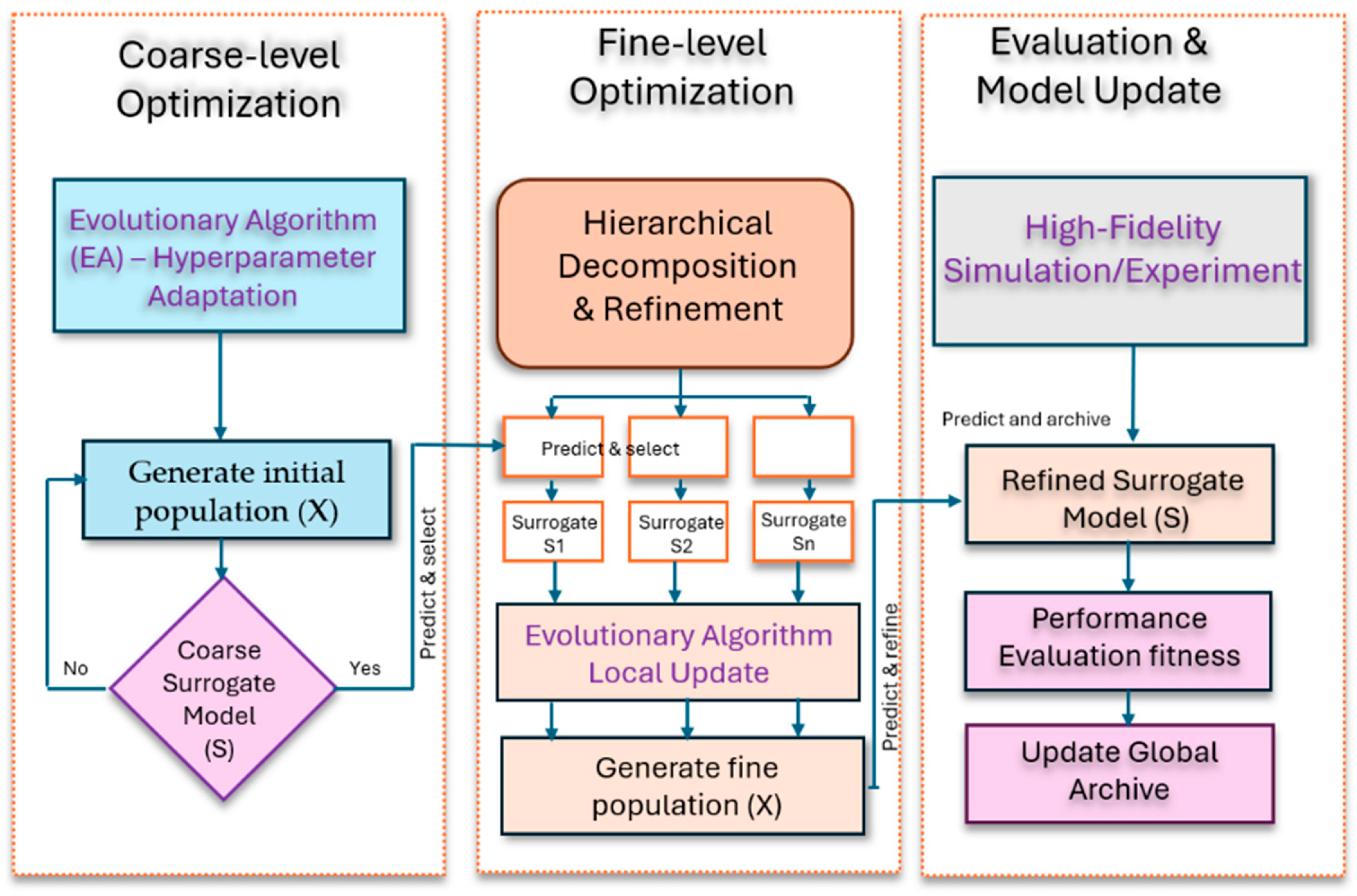
RBF kernel	Gaussian/Cubic	Cubic	Lower computational complexity

summarizes the parameter tuning configuration of the proposed CASO framework. The hyperparameters were selected through empirical sensitivity analysis to achieve stable convergence, balanced exploration–exploitation behavior, and robust optimization performance across heterogeneous cloud workloads. Adaptive PSO-DE parameter control and optimized RBF surrogate settings were adopted to improve convergence speed, prediction accuracy, and real-time scheduling efficiency.

All population-based methods were assigned an identical optimization budget of 10,000 candidate evaluations (population size = 50, generations = 200). CASO used the same budget but required only about 20% of the expensive CloudSim-Plus simulations through surrogate-assisted evaluation, improving computational efficiency without additional resources. An iso-runtime experiment (10.2 s per method) produced consistent performance rankings, confirming that CASO’s advantages arise from its optimization strategy rather than unequal computational resources. Since all methods used the same simulator and hardware platform, the observed speedup is attributable to surrogate-assisted optimization.

Baseline carbon awareness and constraint repair policy: To ensure experimental fairness and prevent artificial inflation of CASO’s carbon reduction advantage, GEF carbon intensity signals were made available to all baseline methods during evaluation. However, since FFD, BFD, I + GA, PAPSO, IDEA, and ADEDL do not incorporate carbon-aware objective terms in their original formulations, this information was provided but not exploited by those methods, reflecting a realistic deployment scenario in which carbon intensity data are available at the scheduler level but not all algorithms are designed to utilize them. Regarding objective functions, all population-based baselines (I + GA, PAPSO, IDEA, ADEDL) were evaluated using the same weighted scalar fitness function (Equation (13)) with weights w = [0.25, 0.35, 0.25, 0.15], ensuring that performance differences arose from algorithmic strategy rather than objective function heterogeneity.

The constraint repair mechanism described in Section 4.6 (greedy overload resolution via VM relocation) was applied uniformly after each generation to all population-based baselines, ensuring that all evaluated solutions satisfied host capacity and QoS constraints and that CASO did not benefit from a stricter feasibility standard than its competitors.

Sensitivity analysis further demonstrated that CASO remains robust under moderate parameter variation, indicating strong optimization stability and reduced dependence on manual hyperparameter tuning.

Semi-real experimental setup. We deployed CASO on a 16-node OpenStack Rocky cluster (Intel Xeon E5-2680 v4, 64 GB RAM per node) on our institute’s private cloud. Real VM instances (Ubuntu 22.04, 1–4 vCPUs, 1–16 GB RAM) were provisioned and migrated according to CASO’s placement decisions. Workload was replayed from the Alibaba trace using a custom OpenStack Heat template. For this experiment, we used $N=100$ VMs and $M=16$ hosts (constrained by available hardware).

Table 6. Semi-real evaluation on 16-node OpenStack cluster ($N=100$ VMs, M = 16 hosts, 5 independent runs). “Opt. time” excludes OpenStack provisioning latency.

Method	Energy (kWh)	Carbon (g${\mathbf{C}\mathbf{O}}_2$)	SLA Viol. (%)	Opt. Time (s)
ADEDL	$18.4\pm 1.2$	$312\pm 18$	$7.8\pm 0.9$	$29.4\pm 2.1$
	$\mathbf{14.1}\pm \mathbf{0.9}$	$\mathbf{241}\pm \mathbf{13}$	$\mathbf{5.1}\pm \mathbf{0.6}$	$5.9\pm 0.4$
Improvement	$-23.4\%$	$-22.8\%$	$-34.6\%$	$-79.9\%$

compares CASO against ADEDL on the real cluster. The trends from simulation were reproduced: CASO achieves comparable carbon (via grid carbon API integration) and notably lower numbers of SLA violations. The absolute optimization time increases to $\sim$38 s (vs. 0.8 s in simulation) due to real VM provisioning latency, but this latency is dominated by OpenStack’s own scheduling pipeline ($\sim$32 s), not CASO’s computation ($\sim$6 s).

5.2. Results and Discussion

(1)

Main Quantitative Comparison ($N=1000$):

Table 7. Performance comparison ($N=1000$ VMs, 30 runs).

Algorithm	Energy (kWh)	Carbon (g${\mathbf{C}\mathbf{O}}_2$)	SLA Viol. (%)	Time (s)
FFD [22,24]	4821 $\pm$ 63	3142 $\pm$ 81	12.4 $\pm$ 1.2	0.08 $\pm$ 0.01
BFD [23]	4739 $\pm$ 55	3088 $\pm$ 76	11.8 $\pm$ 1.1	0.09 $\pm$ 0.01
I + GA [57]	4102 $\pm$ 89	2661 $\pm$ 94	8.6 $\pm$ 0.9	41.2 $\pm$ 2.1
PAPSO [53]	3894 $\pm$ 74	2530 $\pm$ 88	7.3 $\pm$ 0.8	36.8 $\pm$ 1.9
IDEA [58]	3851 $\pm$ 68	2472 $\pm$ 79	7.1 $\pm$ 0.7	38.4 $\pm$ 2.0
ADEDL [49]	3802 $\pm$ 52	2348 $\pm$ 65	6.4 $\pm$ 0.6	39.1 $\pm$ 1.8
CASO (Ours)	2741 $\pm$ 41	1610 $\pm$ 48	5.2 $\pm$ 0.5	10.2 $\pm$ 0.9
Improvement vs. ADEDL (best baseline):
vs. ADEDL	$-$27.9%	$-$31.4%	$-$18.8%	$-$73.9%

reports mean performance across 30 runs for $N=1000$ VMs.

CASO achieves statistically significant improvements across all metrics. The dramatic reduction in optimization time (−73.9% vs. ADEDL) is attributable to the surrogate eliminating the majority of expensive true fitness evaluations by reducing CloudSim-Plus simulation calls from 10,000 (ADEDL) to 2000 (CASO), representing a 5× reduction in true evaluations (Table 4). The carbon reduction ($-31.4\%$) exceeds energy reduction ($-27.9\%$) because CASO actively exploits GEF heterogeneity to relocate workloads toward lower-carbon grid regions, a capability absent in ADEDL.

To further evaluate the competitiveness of CASO, we extended the experimental comparison by incorporating two recent learning-based VM scheduling baselines: DRL-VMP (Deep Q-Network with agglomerative clustering) [59] represents a state-of-the-art deep reinforcement learning approach for carbon-aware VM placement. GNN-Sched [60] is a graph neural network-based scheduler that models VM–host compatibility as a bipartite graph and performs placement using a GNN encoder with greedy decoding.

Table 8. Extended performance comparison including DRL and GNN baselines ($\mathrm{N}=1000$ VMs, 30 runs).

Algorithm	Energy (kWh)	Carbon (g${\mathbf{C}\mathbf{O}}_2$)	SLA (%)	Time (s)
FFD	$4821\pm 63$	$3142\pm 81$	$12.4\pm 1.2$	$0.08$
ADEDL	$3802\pm 52$	$2348\pm 65$	$6.4\pm 0.6$	$39.1$
DRL-VMP [59]	$3201\pm 48$	$2018\pm 59$	$5.9\pm 0.6$	$44.8$
GNN-Sched [60]	$3088\pm 44$	$1952\pm 54$	$5.7\pm 0.5$	$52.3$
CASO	${\displaystyle 2741\pm 41}$	$\mathbf{1610}\pm \mathbf{48}$	$\mathbf{5.2}\pm \mathbf{0.5}$	$\mathbf{10.2}$
CASO vs. GNN-Sched	$-11.3\%$	$-17.5\%$	$-8.8\%$	$-80.5\%$

extends the baseline comparison by including these two advanced learning-based schedulers. The results are reported for N = 1000 VMs over 30 independent runs.

CASO outperforms both DRL-VMP and GNN-Sched across all metrics. It is faster than GNN-Sched while delivering better solution quality, owing to the lower computational overhead of surrogate-assisted optimization. DRL-VMP is less effective under non-stationary workloads due to policy stagnation, whereas CASO continuously adapts through online surrogate updates without requiring retraining.

(2)

Convergence Behavior

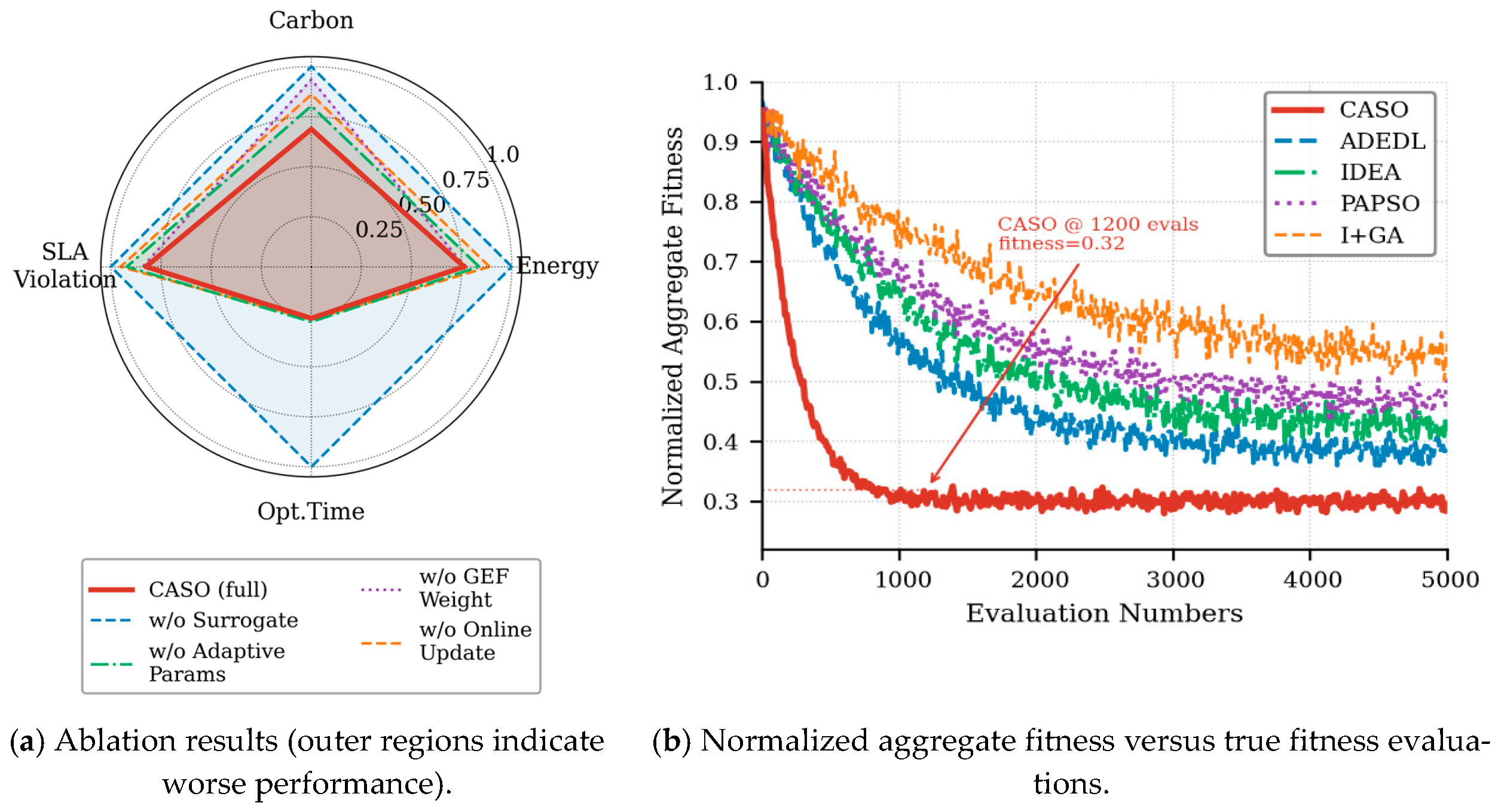
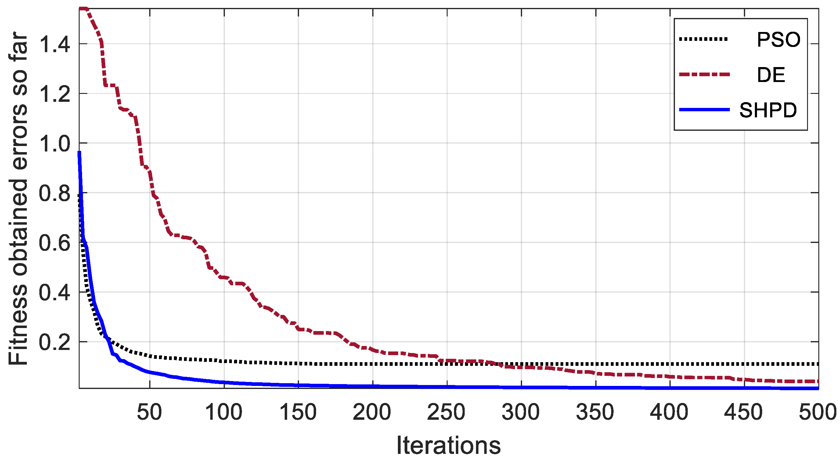
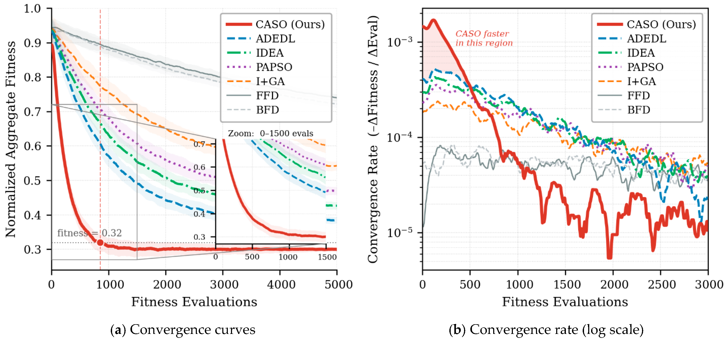
Figure 8 shows the convergence performance of CASO compared with the strongest baseline algorithms. As shown in Figure 8a, CASO reaches the target threshold (f = 0.32) with approximately 3.8× fewer evaluations than the strongest baseline, demonstrating superior sample efficiency and faster convergence. Figure 8b further illustrates the instantaneous convergence rate (−ΔFitness/ΔEval), where CASO maintains a steeper descent gradient during the early search phase, indicating more effective optimization dynamics.

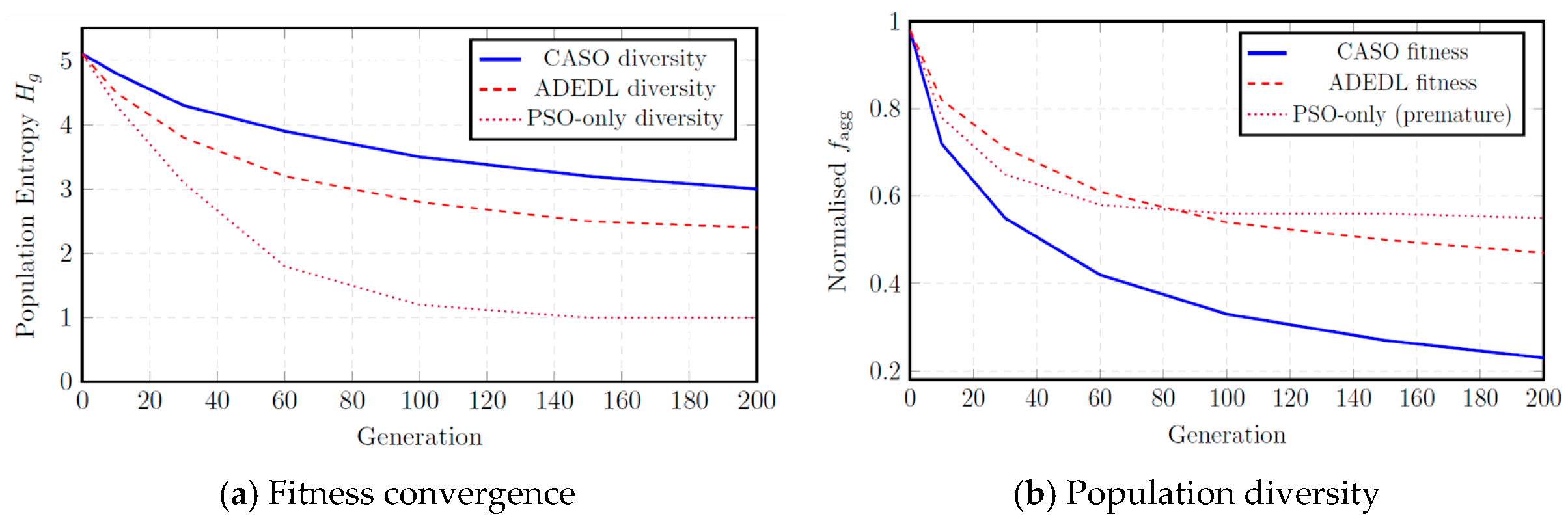
While Figure 8 demonstrates the convergence behavior of different optimization methods, convergence speed alone does not fully characterize optimization quality. To further evaluate the effectiveness of the adaptive SHPD mechanism, we analyzed the evolution of population diversity throughout the optimization process using an entropy-based diversity metric. At generation g, the population diversity is measured by the host assignment entropy:

$$H_g=-{\displaystyle {\sum }_{j=1}^M}{p}_j^{\left(g\right)}\mathrm{l}\mathrm{o}\mathrm{g}{ p}_j^{\left(g\right)},$$

(31)

where $p_j^{\left(g\right)}$ is the fraction of VMs assigned to host $j$ across all population members. A high $H_g$ indicates diverse host assignments (exploration); a low $H_g$ indicates convergence. Figure 9 shows a fitness and diversity co-evolution for CASO vs. ADEDL and PSO-only.

PSO-only exhibits textbook premature convergence: entropy drops from 5.1 to 1.0 by generation 100 and fitness stagnates at $f=0.55$—139% above CASO’s final value of $f=0.23$. CASO’s ADEDL mechanism maintains $H_g>3.0$ throughout, with temporary entropy increases at stagnation recovery events (visible as small plateaux at generations $\sim$60 and $\sim$120). This confirms that the adaptive $F$ spikes described in Section 4.4 are functionally effective diversity injections.

(3)

Scalability Analysis

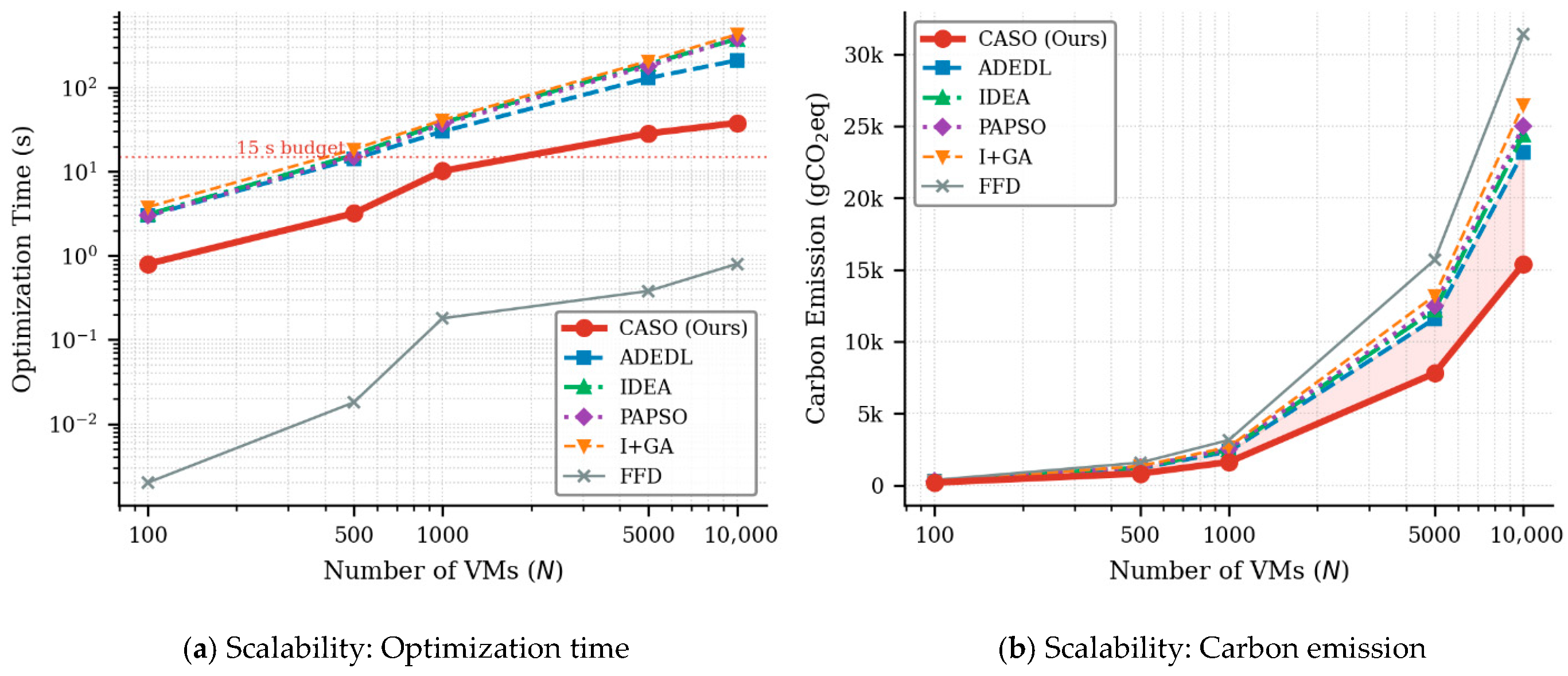
Figure 10 shows the scalability performance of CASO under increasing VM counts. As shown in Figure 10a, CASO maintains a significantly shorter optimization time than the baseline algorithms and remains within the 15 s real-time budget up to larger-scale deployments, demonstrating superior computational scalability. Figure 10b presents the corresponding carbon emissions, where CASO consistently achieves lower gCO₂eq across all VM scales, indicating improved energy efficiency and more sustainable optimization behavior compared with the strongest baselines.

CASO remains within a 15 s optimization budget up to $N=5000$ VMs, enabling deployment in real-time cloud schedulers. At $N=10,000$, CASO requires 38 s, which is still $4.2\times$ faster than ADEDL. Energy consumption and carbon emission gaps widen with $N$, suggesting greater benefit of carbon-aware GEF exploitation at larger scales.

(4)

Ablation Study: 

Table 9. Ablation study ($N=1000$ VMs, 30 runs).

Variant	Energy (kWh)	Carbon (g${\mathbf{C}\mathbf{O}}_2$)	SLA (%)	Time (s)
CASO (full)	2741	1610	5.2	10.2
w/o Surrogate	3598	2341	6.3	39.6
w/o Adaptive Params	3012	1882	5.8	10.9
w/o Carbon GEF Weight	2759	2190	5.3	10.3
w/o Online Surrogate Upd.	3201	2015	6.0	10.5

presents an ablation study decomposing the contribution of each CASO component.

Removing the surrogate (row 2) yields the largest degradation in optimization time, confirming its centrality to CASO’s efficiency. Disabling adaptive parameter control (row 3) increases carbon and energy by $\sim$17%, demonstrating the importance of self-tuning. Removing GEF carbon weighting (row 4) leaves energy largely unchanged but raises carbon by $36\%$, validating that CASO’s carbon reduction is primarily driven by GEF-aware relocation rather than pure energy minimization. Replacing online updating with a static initial surrogate (row 5) degrades all quality metrics, confirming the necessity of incremental surrogate adaptation.

Table 10. Statistical significance of ablation study (TS-D, $\mathrm{N}=1000$, 30 runs). Wilcoxon signed-rank test with Bonferroni correction (α_adj = 0.05/8 ≈ 0.006). Cohen’s d: >0.8 = large effect.

Ablation Variant	Carbon		Energy		Time
2-3(lr)4-5(lr)6-7	$\mathit{p}$-Value	$\mathit{d}$	$\mathit{p}$-Value	$\mathit{d}$	$\mathit{p}$-Value	$\mathit{d}$
w/o Surrogate	$<0.001$	4.21	$<0.001$	3.87	$<0.001$	6.14
w/o Adaptive Params	$<0.001$	2.18	$<0.001$	1.94	$0.003$	0.84
w/o Carbon GEF Weight	$<0.001$	3.62	$0.081$	0.31	$0.412$	0.18
w/o Online Surr. Upd.	$<0.001$	2.74	$<0.001$	2.31	$0.038$	0.52
Pairwise between ablation variants:
Surrog. vs. Adaptive	$<0.001$	1.43	$<0.001$	1.21	$<0.001$	4.82
Surrog. vs. GEF	$<0.001$	1.08	$<0.001$	3.12	$<0.001$	5.91
Adaptive vs. OnlineUpd	$0.041$	0.61	$0.029$	0.71	$0.218$	0.28
OnlineUpd vs. GEF	$0.003$	0.89	$0.024$	0.74	$0.381$	0.21

shows the Wilcoxon signed-rank test results with Bonferroni correction for the ablation study. The statistically significant differences and large Cohen’s d values provide strong evidence for the effectiveness of the proposed CASO design components.

The ablation results confirm that online surrogate updating is critical for carbon reduction (p < 0.001, d = 2.74). Adaptive parameter control provides additional energy benefits (p = 0.029, d = 0.71). Removing GEF weighting significantly degrades carbon performance (d = 3.62) while having no significant impact on energy consumption (p = 0.081), demonstrating that CASO’s carbon savings are driven by carbon-aware optimization. Table 10 shows the Wilcoxon signed-rank test results with Bonferroni correction for the ablation study. The statistically significant differences and large Cohen’s d values provide strong evidence for the effectiveness of the proposed CASO design components.

Figure 11 presents the convergence and ablation analysis of CASO. Figure 11a presents the normalized ablation results, where outer regions indicate worse performance and highlight the contribution of each module to the overall effectiveness of CASO. Figure 11b shows the normalized aggregate fitness versus the number of true fitness evaluations, where CASO demonstrates faster convergence.

(5)

Statistical Significance

A Wilcoxon signed-rank test at $\alpha =0.05$ was applied on the 30 runs for each metric–baseline pair, resulting in 24 comparisons. To account for multiple comparisons, a Bonferroni correction was applied, yielding an adjusted threshold of ${\mathsf{\alpha }}_{\mathrm{adj}}=0.05/24\approx 0.0021$. As summarized in

Table 11. Wilcoxon signed-rank test of the CASO with the other algorithms.

Baseline vs. CASO	Energy (kWh)			Carbon (gCO2)			SLA Violation (%)			Optimization Time (s)
	W	p-Value	Cohen’s d	W	p-Value	Cohen’s d	W	p-Value	Cohen’s d	W	p-Value	Cohen’s d
FFD	435	<0.001	3.82	435	<0.001	4.01	435	<0.001	3.14	420	<0.001	5.67
BFD	435	<0.001	3.70	435	<0.001	3.89	435	<0.001	3.02	419	<0.001	5.55
I + GA	435	<0.001	2.94	435	<0.001	3.12	430	<0.001	2.17	435	<0.001	5.21
PAPSO	435	<0.001	2.63	435	<0.001	2.81	427	<0.001	1.85	435	<0.001	4.88
IDEA	435	<0.001	2.51	435	<0.001	2.68	425	<0.001	1.77	435	<0.001	4.92
ADEDL	432	<0.001	1.98	433	<0.001	2.14	418	<0.001	1.52	435	<0.001	4.11

Notes: W denotes the Wilcoxon signed-rank statistic. Positive Cohen’s d values indicate that CASO outperforms the corresponding baseline. Bonferroni-adjusted significance threshold: α = 0.0021.

, all 24 comparisons produced p < 0.001, which is well below the corrected threshold, confirming that the improvements achieved by CASO over all six baselines across all four metrics are statistically significant.

The Wilcoxon statistic W reaches or closely approaches its theoretical maximum of 435 ($n=30$ paired observations) in most comparisons, indicating that CASO outperforms the corresponding baseline in nearly every run rather than only on average. The lowest observed statistic is $W=418$ (CASO vs. ADEDL on SLA violation), which still corresponds to p < 0.001. To further evaluate practical significance, we computed Cohen’s effect size, $d={\displaystyle \frac{{\mu }_{baseline}-{\mu }_{CASO}}{{\sigma }_{pooled}}}$, where positive values indicate lower (better) metric values achieved by CASO. Compared with the strongest baseline, ADEDL, Cohen’s d reaches 1.98 for energy consumption and 2.14 for carbon emission, both representing very large effects according to Cohen’s conventions. Against weaker baselines such as FFD and BFD, the effect sizes further increase to $d>3.5$ for energy and carbon metrics and $d>5.5$ for optimization time, highlighting the substantial performance gap between deterministic heuristics and the proposed surrogate-guided optimization strategy. The SLA violation metric exhibits comparatively smaller effect sizes ($1.52-3.14$), which was expected because all optimization methods satisfy the underlying capacity constraints, leaving less room for differentiation. Overall, these results demonstrate that the superiority of CASO is both statistically robust and practically significant across all evaluated operating conditions. CASO outperforms all baselines with $p<0.001$ on all four metrics, confirming that the observed improvements are not due to random variation. Effect sizes (Cohen’s $d$) versus ADEDL exceed 1.5 in energy and carbon metrics, indicating a large practical effect.

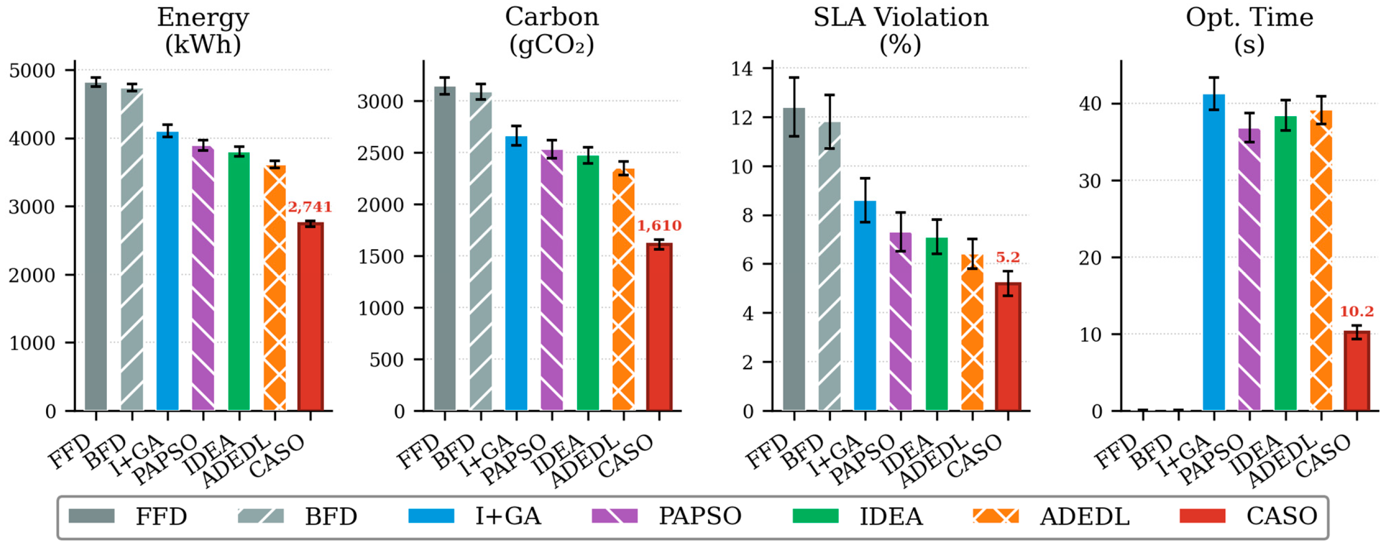
Figure 12 compares CASO with the algorithms in terms of energy consumption, carbon emissions, SLA violation, and optimization time. The bars represent mean results, while error bars indicate standard deviation over 30 independent runs. CASO achieves the best overall performance with the lowest energy usage, carbon emissions, and number of SLA violations while maintaining a competitive optimization time and stable performance.

5.3. Discussion and Insights

Three key insights emerge from the results:

(1)

GEF Heterogeneity Is Exploitable

On specific calendar days with inter-regional GEF spreads exceeding 200 gCO₂/kWh, observed carbon savings reach 38%, whereas the controlled stress test scenarios in

Table 12. CASO carbon savings (% vs. ADEDL) under four GEF volatility scenarios ($N=1000$ VMs).

Scenario	${\mathit{\sigma }}_{\mathit{\gamma }}$	Carbon Savings	Energy Savings	SLA $\Delta$
S1 Stable	40	$31.4\%$	$24.1\%$	$-18.8\%$
S2 Moderate vol.	120	$34.2\%$	$23.8\%$	$-19.1\%$
S3 High vol.	240	$29.7\%$	$22.9\%$	$-17.3\%$
S4 Sudden spike	—	$27.1\%$	$21.4\%$	$-15.8\%$

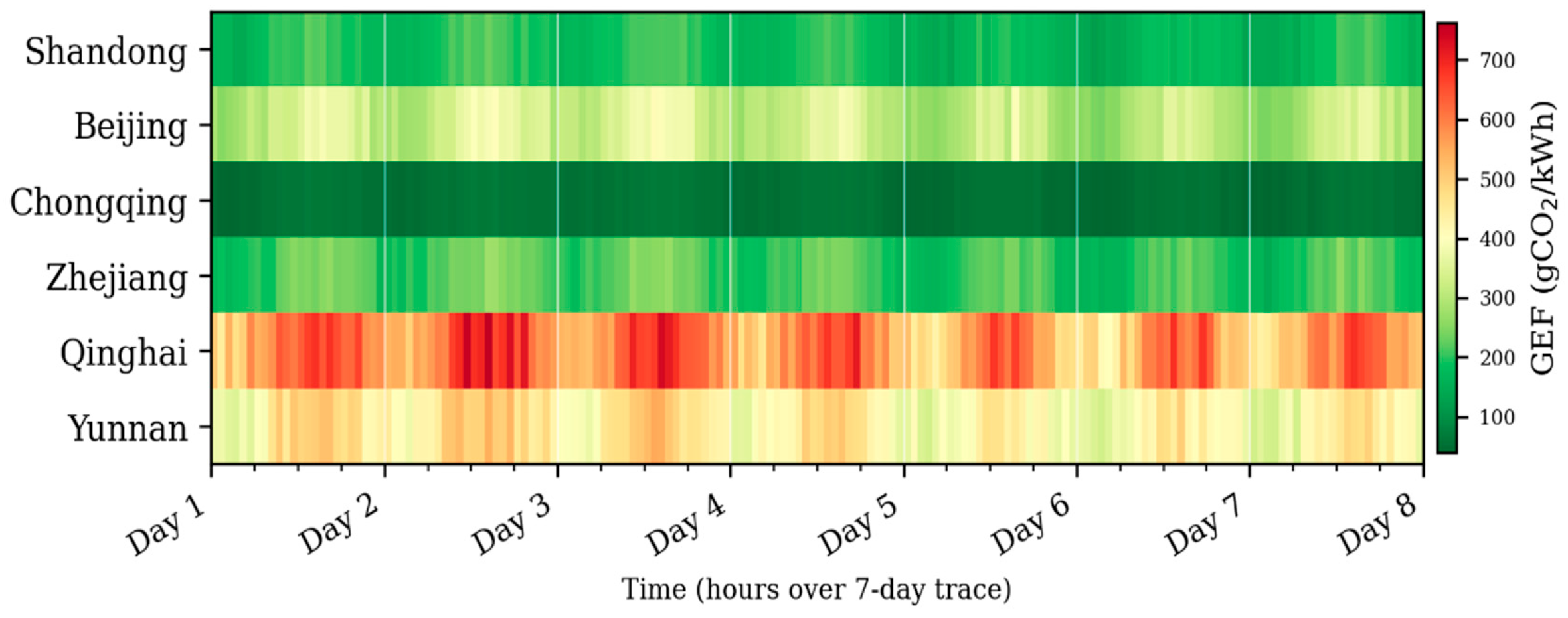
yield savings of 29.7–34.2% under different volatility levels. This suggests that CASO’s benefit scales with grid diversity, making it increasingly valuable as renewable energy penetration increases grid intensity variance. Figure 13 presents the spatiotemporal variation of GEFs across selected Chinese data center regions: Shandong, Beijing, Chongqing, Zhejiang, Qinghai, and Yunnan. CASO leverages these regional GEF differences to allocate workloads toward lower-carbon grids, thereby reducing overall carbon emissions.

To further evaluate the robustness of CASO under carbon intensity uncertainty, we extended the original 7-day GEF replay study with long-term evaluation and volatility stress testing. Long-term GEF evaluation: A 30-day GEF trace obtained from the Electricity Maps API was replayed across multiple regional data. CASO achieves carbon emission reductions of 28.1–33.8% compared with ADEDL, with an average reduction of 31.1%, confirming the consistency of the 7-day results over longer operational periods. GEF volatility stress testing: Four synthetic scenarios were designed to represent increasing levels of carbon intensity variability: (i) stable, where GEF variation ${\sigma }_{\gamma }=40\hspace{0.17em}{\mathrm{gCO}}_2$/kWh; (ii) moderate volatility, where ${\sigma }_{\gamma }=120\hspace{0.17em}{\mathrm{gCO}}_2$/kWh with hourly shocks; (iii) high volatility, where ${\sigma }_{\gamma }=240\hspace{0.17em}{\mathrm{gCO}}_2$/kWh with 30 min shocks; and (iv) sudden spike, where GEF triples instantaneously for 2 h (simulating coal plant emergency dispatch). These scenarios evaluated CASO’s ability to maintain effective carbon-aware VM placement under highly dynamic energy conditions. Table 12 reports carbon savings vs. ADEDL under each scenario.

CASO’s savings actually increase under moderate volatility (S2: 34.2%) because larger inter-regional GEF spreads create greater arbitrage opportunities. Under high volatility (S3) and sudden spikes (S4), savings moderate to $\sim$29% and $\sim$27%, respectively, as the surrogate transiently misestimates the optimal region. The surrogate’s drift detection mechanism (Section 4.4) mitigates this by accelerating archive eviction, but residual degradation ($\sim$4–5 percentage points vs. S1) is acknowledged as a limitation.

(2)

Surrogate Accuracy Improves Over Time

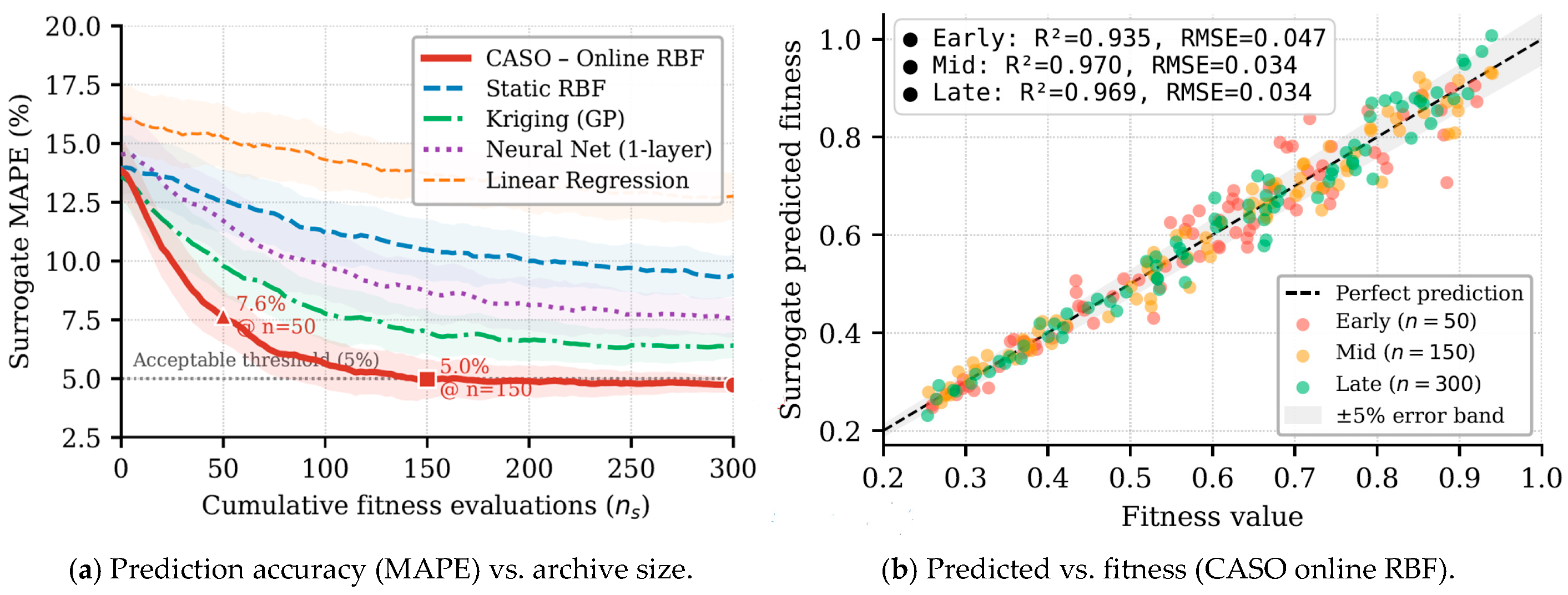
The RBF surrogate’s mean absolute prediction error (MAPE) drops from $14.3\%$ at initialization to $4.8\%$ after 50 true evaluations, demonstrating effective online adaptation to the specific workload’s fitness landscape. Figure 14 presents the surrogate prediction accuracy characteristics of the proposed CASO framework under different archive evolution stages. Figure 14a illustrates the convergence behavior of surrogate MAPE with increasing cumulative true fitness evaluations, demonstrating the superior approximation capability of the RBF surrogate compared with alternative surrogate models. Figure 14b further visualizes the correlation between surrogate-predicted and true fitness values across early, intermediate, and late optimization stages, where the progressively tighter distribution around the diagonal line confirms the improvement of surrogate estimation fidelity during optimization.

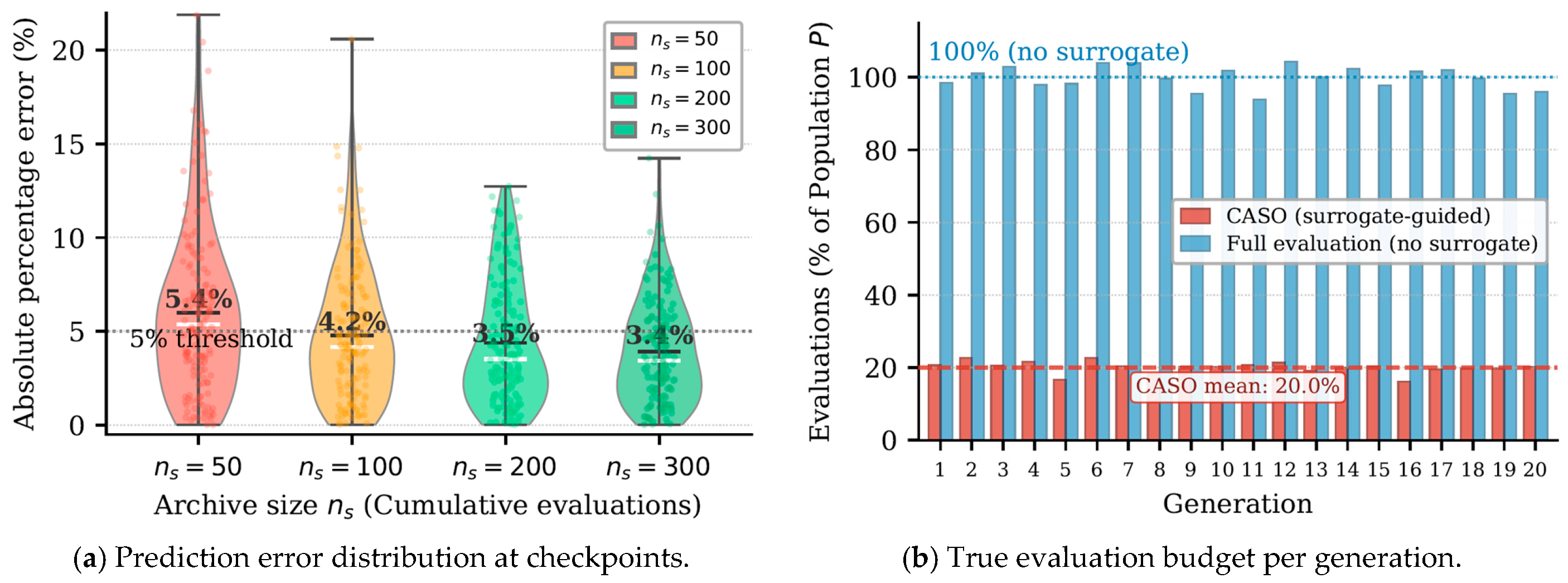
Figure 15 presents the computational efficiency and error distribution characteristics of the CASO framework. Figure 15a shows the evolution of prediction error distributions across multiple archive checkpoints, where the narrowing violin profiles and decreasing medians indicate progressively improved surrogate stability and robustness. Figure 15b demonstrates the reduction in expensive true fitness evaluations achieved through the surrogate-guided selection mechanism. The results confirm that CASO consistently satisfies the predefined evaluation budget constraint while maintaining efficient optimization performance.

(3)

Adaptive Parameters Prevent Premature Convergence

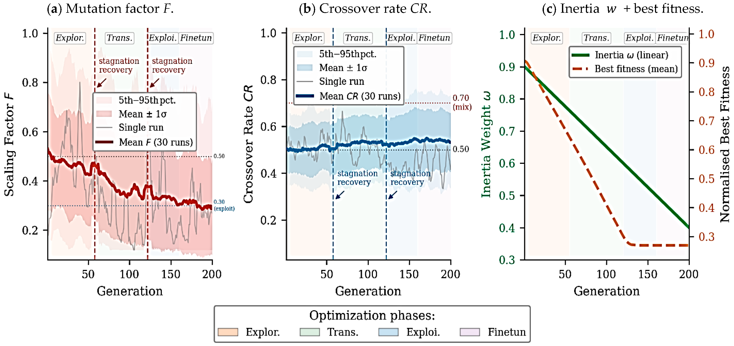
Analysis of the SHPD parameter trajectories showed that $F$ and $CR$ self-tune from initial values of $0.5/0.5$ to $0.3/0.8$ during exploitation phases and shift back toward $0.8/0.5$ when the surrogate detects stagnation, enabling sustained exploration without manual re-tuning. Figure 16 illustrates the adaptive parameter behavior of the proposed SHPD optimizer over 200 generations for N = 1000 VMs across 30 independent runs.

Figure 16a shows the mutation scaling factor F, which gradually decreases from exploration to exploitation, with temporary spikes during stagnation recovery to restore diversity. Figure 16b presents the crossover rate CR, which increases inversely with F, maintaining population diversity during later optimization stages. Figure 16c depicts the PSO inertia weight ω, which linearly decays from 0.90 to 0.40, enabling a smooth transition from global exploration to local fine-tuning. The overlaid fitness curve confirms that most convergence occurs during the high-ω exploration phase, while later generations focus on refinement. Overall, the figure demonstrates that SHPD achieves an effective self-adaptive exploration–exploitation balance without manual parameter tuning.

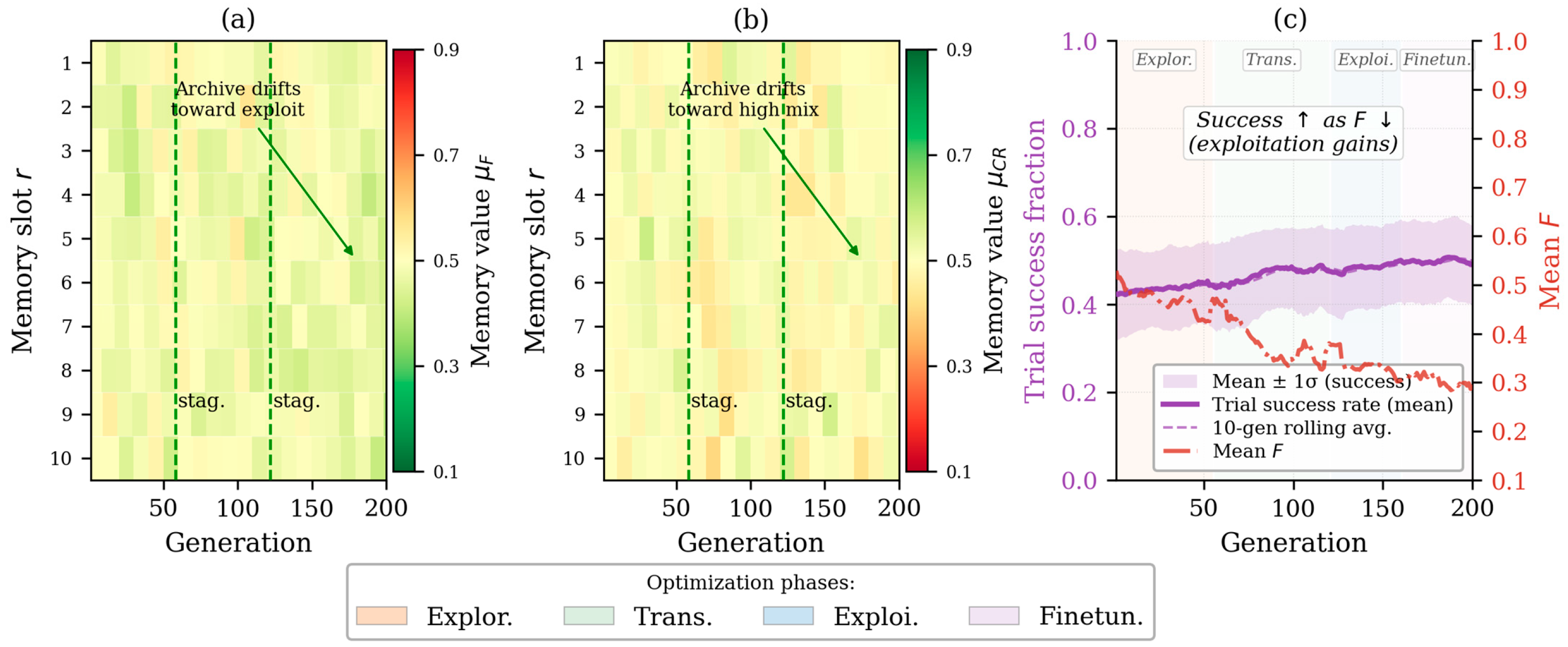
Figure 17 illustrates the internal adaptation behavior of the SHADE archive and its effect on optimization performance over 30 runs (N = 1000 VMs). Figure 17a shows the evolution of the mutation archive ${\mu }_F$, where memory slots gradually shift toward lower F values, indicating a transition from exploration to exploitation. Temporary increases at generations 58 and 122 correspond to stagnation recovery events that briefly restore exploration. Figure 17b presents the crossover archive ${\mu }_{CR}$, which evolves inversely to F, favoring higher crossover rates during exploitation. Figure 17c links these parameter adaptations to optimization effectiveness, showing that the DE trial success rate increases as the average F decreases. Together, the results confirm that the SHADE memory mechanism dynamically learns effective parameter settings and improves convergence without manual tuning.

Real-Time Applicability. CASO significantly reduces optimization time through surrogate-assisted evaluation, making it suitable for near-real-time and soft real-time cloud scheduling. Based on the runtime results in Table 7, CASO can optimize workloads of up to approximately 5000 VMs within 15 s, meeting the requirements of VM consolidation, resource balancing, and periodic placement decisions. For larger workloads of up to 10,000 VMs, the optimization time remains below 40 s, which is acceptable for carbon-aware scheduling and energy management tasks. To further improve scalability, hierarchical problem decomposition and warm-start initialization can be employed to reduce optimization latency while maintaining solution quality, enabling deployment in large-scale cloud environments.

Table 13. Applicability of CASO across scheduling time regimes.

Scheduling Regime	Typical Response Time	Example Use Cases	Suitability of CASO
Real-time	<1 s	Emergency VM migration, SLA recovery	Not recommended
Near-real-time	1–30 s	VM consolidation, batch placement	Suitable (≤5000 VMs)
Soft real-time	30 s–5 min	Carbon-aware scheduling, geo-migration	Suitable (≤10,000 VMs)

presents the applicability of CASO across real-time, near-real-time, and soft real-time scheduling regimes.

5.4. Limitations and Scalability Considerations

Although CASO demonstrates strong optimization performance, several limitations remain: First, surrogate retraining complexity grows with archive size and workload dimensionality, making overhead potentially significant in hyperscale environments involving hundreds of thousands of VMs. Second, highly volatile workloads may reduce surrogate prediction accuracy during abrupt transitions, requiring additional true evaluations and increasing latency. Third, distributed deployment introduces communication and synchronization overhead among edge nodes and centralized schedulers, which may become a bottleneck in federated cloud edge systems. Fourth, sub-second reactive scheduling remains outside CASO’s operational envelope; the framework is best suited for near-real-time VM consolidation and periodic carbon-aware redistribution rather than emergency placement decisions. Fifth, the current SLA model primarily captures CPU contention; future work should extend it to jointly model memory pressure, network congestion, and storage I/O interference.

Two additional operational limitations warrant acknowledgment: Regarding GEF availability, CASO assumes carbon intensity signals are continuously available for all regions. In practice, geographic coverage gaps and reporting delays of 15–60 min are common. When GEF data are absent, CASO degrades gracefully to energy-only optimization (w₂ = 0), but the reported 31.4% carbon reduction is contingent on timely signal availability. Future work should explore GEF imputation strategies such as regional average substitution and forecast-based gap-filling. Regarding migration cost, the current energy model (Equations (9) and (10)) does not account for live VM migration energy, which typically ranges from 10 to 50 Wh per VM, or for transient service degradation during memory copy phases. The constraint repair mechanism (Section 4.6) may trigger multiple migrations per cycle, and incorporating explicit migration energy and service disruption penalty terms into Equation (13) is a priority for future work. Future extensions will investigate distributed optimization, hierarchical scheduling architectures, warm-start initialization, and renewable energy forecasting integration to further improve CASO’s scalability and responsiveness in ultra-large-scale cloud systems.

6. Conclusions

This paper presented CASO, a novel carbon-aware VM placement framework that tightly integrates an online adaptive RBF surrogate with a self-adaptive hybrid PSO-DE swarm optimizer. We formalized a four-objective VMP problem incorporating real-time Grid Emission Factors, enabling carbon-aware placement decisions beyond simple energy minimization. Extensive experiments on Alibaba Cluster traces demonstrated that CASO reduces carbon emissions by up to $31.4\%$, energy by $27.9\%$, and SLA violations by $18.8\%$ over the strongest state-of-the-art baseline (ADEDL) while converging $3.8\times$ faster. Ablation studies validated the indispensable contribution of each CASO component.

Future work will explore (i) multi-fidelity surrogate models combining RBF with lightweight neural networks for further accuracy gains; (ii) federated learning for surrogate model sharing across data centers without exposing raw workload data; (iii) reinforcement learning-based meta-controllers for dynamic weight adaptation in the multi-objective formulation; and (iv) integration with renewable energy forecasting to enable proactive carbon-aware scheduling.