Spatiotemporal Dynamics and Drivers of Hydroclimatic Change in the Mu Us Sandy Land: A Machine Learning and Multi-Scale Analysis

Abstract

Climate change remains among the most pressing environmental challenges confronting the world, exerting profound pressure on both ecological systems and socio-economic development. To advance understanding of the evolution patterns and driving mechanisms governing hydroclimatic systems in arid and semi-arid regions, this study employed an integrated framework encompassing trend testing, change-point detection, periodicity and persistence analysis, and machine learning-based attribution. Focusing on the Mu Us Sandy Land from 1982 to 2023, we systematically investigated the spatiotemporal evolution, periodic characteristics, and driving mechanisms of hydroclimatic factors. Furthermore, future climate risks were assessed using CMIP6 multi-model data. The results showed that: (1) All four variables exhibited positive slopes, but only soil moisture showed a statistically significant long-term wetting trend (β = 0.025 × 10⁻³, p = 0.0008) and a clear global abrupt change in 2011; the upward tendencies of precipitation (p = 0.3946), potential evapotranspiration (p = 0.4970), and surface runoff (p = 0.1097) did not reach the 0.05 significance level. (2) Meteorological elements showed weak periodicity and strong anti-persistence (mean Hurst index = 0.379 for precipitation and 0.222 for PET), whereas hydrological elements exhibited clear seasonal–interannual periods and more random future variability with greater spatial heterogeneity (mean Hurst index = 0.436 for runoff and 0.414 for soil moisture). (3) Monthly changes were mainly associated with local surface processes. Vegetation dynamics were key predictors of precipitation, runoff, and soil moisture, while potential evapotranspiration was dominated by atmospheric demand, with limited influence from large-scale climate indices. (4) Under high-emission scenarios, imbalanced water–heat increases may lead to a higher likelihood of drought conditions.

1. Introduction

Climate change is currently the most serious environmental issue globally, and its effects have been significantly manifested worldwide [1]. Global warming, as one of the profound impacts of human activities on the climate system, is increasing the frequency and intensity of extreme weather events [2]. It has exacerbated climate instability and poses systemic risks to the global ecosystem and socio-economic systems [3]. In the analysis of climate change, the non-uniform evolution of precipitation patterns is a key factor shaping current and future climate conditions [4]. Precipitation, as the core component of the Earth’s water cycle, is dynamically influenced by various factors such as soil moisture [5]. Changes in precipitation affect runoff response through vegetation interception and soil infiltration, thereby exacerbating the risk of urban flooding [6]. Meanwhile, the extreme water imbalance caused by changes in precipitation and evapotranspiration (such as droughts and floods) has posed a double threat to the sustainable development of agriculture [7]. If such disturbances continue to intensify, they may even lead to irreversible changes in the structure and function of the ecosystem, threatening the provision of critical ecosystem services at both regional and global scales [8]. Therefore, revealing the spatiotemporal evolution patterns of meteorological and hydrological elements such as precipitation is of considerable practical significance for maintaining regional ecological security, safeguarding water and soil resources, and promoting sustainable management of ecosystems.

China is an important country in the East Asian monsoon region and is one of the regions most vulnerable to extreme hydrological events such as floods and droughts [9]. The sixth assessment report of the IPCC states that the current rate of global warming has substantially surpassed historical observation records [10]. In this context, the temperature in China has exhibited a significant upward trend, with the increase exceeding the global average [11]. Ecologically sensitive areas, especially those in arid and semi-arid regions, respond particularly strongly to climate change. These areas possess fragile environments and unstable systems, and are more vulnerable to degradation processes such as desertification and soil erosion induced by climate change [12]. Observations from the China Meteorological Administration further indicate that as the climate continues to warm, the intensity and duration of extreme weather events are both increasing [13]. Therefore, systematic research on the climate evolution in arid and semi-arid regions has become an important research priority in the field of global environmental change. These regions not only respond to the overall global trend but also exhibit unique regional characteristics, which urgently require in-depth exploration.

The Mu Us Sandy Land (MUSL) is located in northern China and is a typical area with fragile ecology and an important ecological barrier [14]. Although the vegetation restoration in this area has achieved remarkable results, it still faces multiple pressures including the intensification of water shortages, coal development, population growth and rapid urbanization [15]. Under the combined influence of human activities and global change, the interaction between regional ecological and social systems has become increasingly complex, and conflicts have become more prominent, seriously hindering sustainable development [16]. Previous meteorological and hydrological investigations of the MUSL relied on satellite remote sensing, machine learning techniques, or CMIP6 outputs to characterize regional climate dynamics [17,18]. Others employed hydrological models to project environmental changes under climate change scenarios [19]. Although these studies provided valuable insights, they were largely confined to discrete temporal analyses or single-method approaches, while lacking systematic exploration of spatial pattern evolution and their nonlinear driving mechanisms. High-resolution, multi-dimensional assessments of sandy land hydroclimatic conditions therefore remained insufficient. To address this deficiency, the unique contribution of this study lies in: integrating the Mann–Kendall test, Pettitt mutation detection, wavelet analysis, Hurst index, and the LightGBM machine learning model into a unified framework. Compared to traditional single methods, this framework could simultaneously identify trends and mutations, quantify multi-scale cycles, evaluate long-range persistence, and employ LightGBM to reveal multi-factor nonlinear interactions. This not only provided a more comprehensive hydroclimatic evolution picture for the Mu Us Sandy Land, but also offered a transferable methodological paradigm for multi-scale dynamic studies in arid and semi-arid regions.

Based on the above integrated framework, this study focused on MUSL and, using high-resolution three-dimensional datasets, systematically investigated the dynamic evolution patterns of regional hydrometeorological elements from a spatio-temporal integrated perspective. By introducing the Hurst index and multi-model integration methods to assess the persistence characteristics of climate change, and using the LightGBM machine learning model to identify key drivers, the following goals are proposed: (1) To reveal the spatio-temporal patterns and evolution trends of different hydrometeorological elements in MUSL; (2) To clarify its development characteristics and predict the future change direction; (3) To identify the dominant cycles and key drivers of element evolution. This study aimed to systematically depict the spatio-temporal evolution patterns and driving mechanisms of hydrometeorological elements in MUSL. Through high-precision environmental monitoring and ecological risk identification, it provided a scientific basis for the restoration of degraded ecosystems and the rational allocation of water resources, and held practical significance for ensuring ecological security in northern China. The related results can also provide reference methods and theoretical references for the systematic research of similar desertification regions worldwide, and promote innovation in the methods and paradigms of environmental evolution research in arid areas.

2. Study Area and Data

2.1. The Study Area Overview

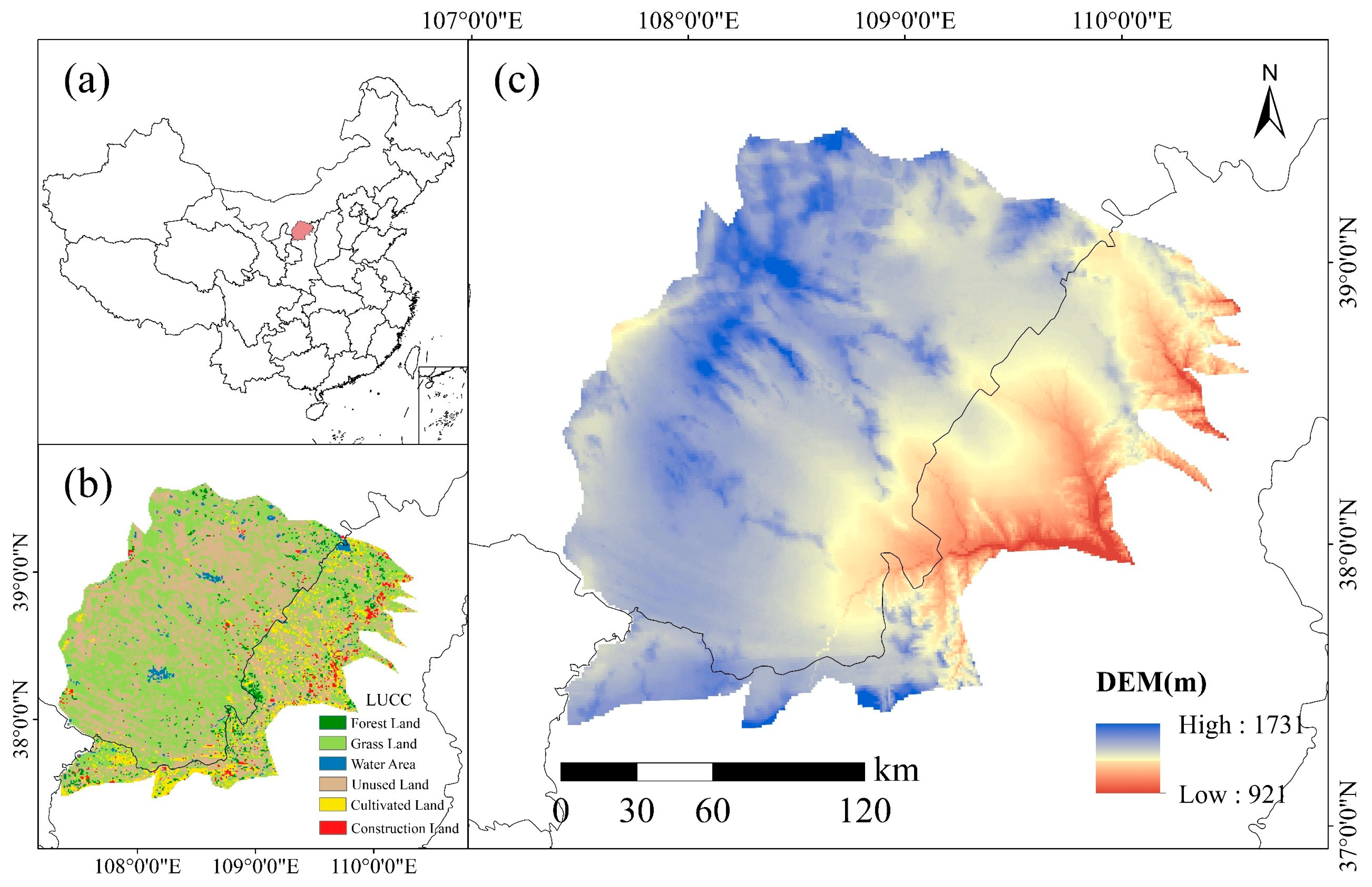
MUSL was situated in northwestern China, at the interface between the Loess Plateau and the Ordos Plateau (Figure 1). It constituted one of the four major semi-arid sandy areas in China, encompassing an area of approximately 40,000 km² [20]. The average altitude of this area ranges from 900 to 1600 m. The overall terrain gradually rises from the northwest to the southeast, and the landform is rather fragmented [16]. Its topography is characterized by the alternating distribution of plateaus, sand dunes and depressions, which was formed under the conditions of a dry climate in the late Quaternary period through the strong wind transportation of ancient river and lake sediment layers [21]. This region lies in the transitional zone between arid and semi-arid areas, as well as between grasslands and desert grasslands. It has a typical semi-arid continental monsoon climate. During the winter and spring seasons, the northwest wind prevails, and the wind erosion effect is significant [22]. Meanwhile, this area is also an important agro-pastoral transitional zone in northern China. The land use types here are complex and the spatial distribution is rather disorderly. In the southern part, agriculture is dominant, while in the northwestern part, animal husbandry is the main form [23]. Under the combined influence of climate change and human activities, the MUSL once suffered from a severe problem of land desertification [24]. Since the 1990s, through the implementation of a series of government-led ecological restoration projects and extensive popularization of sand control activities, the expansion trend of desertification in this region has been effectively curbed. Currently, the measures for vegetation restoration and comprehensive management of sandy areas have achieved remarkable results, and the regional vegetation coverage rate is showing a steady upward trend [16].

2.2. Data Sources

The precipitation and potential evapotranspiration data used in this study are sourced from the National Qinghai–Tibet Plateau Science Data Center (https://data.tpdc.ac.cn/, accessed on 10 October 2025) [25,26]. The runoff and soil moisture data are derived from the NASA FLDAS NOAH dataset and have been applied in multiple studies, demonstrating good credibility (https://disc.gsfc.nasa.gov/, accessed on 10 October 2025) [27,28]. The vapor pressure deficit (VPD) data are sourced from Earth System Science Data (https://essd.copernicus.org/, accessed on 10 October 2025) [29]. In terms of vegetation indices, NDVI was obtained from the figshare repository (https://springernature.figshare.com/, accessed on 10 October 2025) [30]; the leaf area index (LAI) was from the National Cryosphere Desert Data Center (https://www.ncdc.ac.cn/portal, accessed on 10 October 2025) [31]. The atmospheric circulation indices (such as ENSO, SOI, NAO, PDO, etc.) are obtained from the National Center for Atmospheric Research in the United States (https://psl.noaa.gov, accessed on 10 October 2025). The future climate data were sourced from the Coupled Model Intercomparison Project Phase 6 (CMIP6) dataset, and the multi-model ensemble (MME) approach was employed to derive climate projections under different scenarios. All data were uniformly resampled and cropped to a spatial resolution of 0.1° to facilitate the integration and analysis of multi-source datasets. During data processing, rigorous quality control was implemented, with missing-value diagnostics performed both prior to and following computation. Peripheral missing values were imputed via nearest-neighbor differencing or temporal extrapolation, whereas sporadic internal gaps were addressed through spline interpolation or kriging. For future climate projection, monthly output data from eight CMIP6 models were used: ACCESS-CM2, BCC-CSM2-MR, CAS-ESM2-0, CMCC-ESM2, IPSL-CM6A-LR, MPI-ESM1-2-LR, NorESM2-LM, and UKESM1-0-LL. Four hydroclimatic variables were extracted: precipitation, potential evapotranspiration, surface runoff, and soil moisture. The models were selected based on data availability for all four variables from 2015 to 2100 and their common usage in climate impact studies over China. All model outputs were bilinearly interpolated to the same spatial resolution of 0.1° to match the observational datasets used in this study. A multi-model ensemble (MME) was constructed by taking the equally weighted average of the eight models for each variable and scenario. All model outputs were bilinearly interpolated to a spatial resolution of 0.1°. A multi-model ensemble (MME) was constructed by taking the equally weighted average of the eight models for each variable and scenario. Systematic bias correction was not independently performed. The analysis utilized the raw multi-model ensemble mean computed as the equally weighted average of the eight models for each variable and scenario.

3. Methods

3.1. Trend and Abrupt Change Analysis

Hydro-meteorological changes were governed by a confluence of factors encompassing climate change, natural geography, and human activities. Prevalent trend testing methods encompassed the Mann–Kendall, Pettitt, cumulative anomaly, and sliding T-tests, among others [32]. Of these, the Mann–Kendall test (MKT) constituted a non-parametric statistical method extensively employed to detect drought trends [33]. This method imposed no distributional assumptions upon the data and proved insensitive to outliers. To mitigate the impact of sequence autocorrelation on trend identification, this study evaluated various MKT improvement methods and ultimately adopted the trend pre-whitening-adjusted variant to analyze time series trends across hydro-meteorological elements [34]. At a significance level of α = 0.05, p < 0.05 signified a statistically significant trend; |Z| > 1.96 or 2.58 respectively indicated significance at the 95% and 99% confidence levels. The Tau coefficient indicated the direction and magnitude of the trend, with larger absolute values implying a more pronounced trend; the β value quantified the rate of change, with positive values denoting an upward trend. The specific steps of the improved M-K test were as follows: First, the linear trend was removed from the original sequence to yield the detrended sequence, and the significance of its first-order autocorrelation coefficient was assessed. Where the coefficient proved insignificant, the original sequence was tested directly; where significant, the detrended sequence underwent pre-whitening to eliminate autocorrelation, producing an independent sequence. The linear trend component was subsequently restored to this sequence to yield the final series for the MKT.

The Pettitt test (PT) constituted a classic non-parametric method for mutation point detection, employed to pinpoint locations within the time series at which statistical characteristics shifted significantly [35]. This method imposed no distributional assumptions upon the data. It proved applicable to continuous data encompassing hydrological and climatic series, and retained robustness even under small-sample conditions [36]. The core principle entailed identifying structural mutation locations through assessing distributional discrepancies between any two partitions of the sequence. In operational practice, the test pinpointed the most probable mutation point via maximization of the cumulative deviation across preceding and following subsequences, while yielding the corresponding significance probability. Where the test statistic attained the preset significance level (typically p < 0.05), the point was designated as a mutation point, signifying a significant shift in the statistical characteristics (e.g., the mean) of the sequence preceding and following this location [37]. The PT method exhibited robust stability and interpretability. It was endorsed by the World Meteorological Organization and found extensive application in hydro-meteorological abrupt change detection, environmental evolution segmentation, and ecological response analysis. In practical research, this method was frequently coupled with the Mann–Kendall trend test and cumulative anomaly method to reinforce the reliability of abrupt change identification [38].

3.2. Wavelet Analysis

A wavelet was defined as a waveform of finite duration, zero mean, and compact time-domain support. It typically manifested irregular, short-term, and asymmetric properties. Owing to the non-stationary nature of meteorological and hydrological sequences, traditional time-domain or frequency-domain methods proved inadequate in fully resolving their multi-scale time-varying structure. Wavelet-based analysis effectively discerned local anomalies and periodic fluctuations of the sequence within the time-frequency joint domain [39]. The continuous wavelet transform, a representative time-frequency technique, decomposed signals concurrently across temporal and spectral dimensions, affording the resolution of dynamic periodic patterns embedded within both quasi-stationary and non-stationary hydrological regimes. In this study, the continuous wavelet transform was employed to scrutinize monthly meteorological and hydrological sequences, with the objective of identifying dominant oscillation periods and elucidating the temporal evolution of these periodicities [40]. In contrast to the traditional Fourier transform confined exclusively to sine and cosine basis functions, the wavelet transform afforded substantially greater adaptability. Through selection of a mother wavelet conforming to the sequence’s morphological characteristics, local features could be extracted with considerable flexibility. Based on orthogonality properties, wavelet functions were categorized into orthogonal families (e.g., Haar, Daubechies series) and non-orthogonal families (e.g., Morlet, Mexican hat, and Gaussian wavelets), each category proving suited to discrete and continuous analytical contexts, respectively [41]. In climate and hydrological research, the Morlet wavelet emerged as the preferred mother wavelet, attributable to its optimal time-frequency localization and its fidelity in capturing the fluctuation patterns inherent in hydrological sequences [42]. In this study, the complex Morlet wavelet was adopted for continuous wavelet transformation. This function encompassed both real and imaginary components, thereby preserving the full phase information of the signal. Squaring the wavelet coefficients yielded the wavelet power spectrum. Subsequent normalization enabled quantitative comparisons of spectral characteristics across different sequences and scales.

3.3. Hurst Index Analysis

The Hurst Index (HI) served as a pivotal metric for quantifying the long-term dependence and trend persistence of time series, and found extensive application in discerning long-range memory characteristics across hydrological, climatic, and environmental datasets. The R/S analysis (rescaled range analysis), a classical approach to HI estimation, effectively elucidated the fractal architecture and persistent behavior inherent in time series, and proved well-suited to evaluating the memory strength and trend inertia of natural processes across temporal scales [43]. This method was frequently coupled with statistical diagnostics such as the Mann–Kendall trend test to concurrently ascertain the directional trends of historical changes and the likelihood of their future persistence or reversal [44]. Drawing upon the magnitude of the Hurst index, the persistence characteristics of the time series could be classified: at H = 0.5, the sequence constituted a random walk process devoid of long-term memory; for 0 ≤ H < 0.5, the sequence exhibited anti-persistence, with future trends prone to diverge from historical trajectories; the closer H approached 0, the more pronounced the reversal characteristic became; for 0.5 < H ≤ 1, the sequence demonstrated persistence, with historical trends likely to persist; the closer H approached 1, the more stable the trend became and the stronger the predictability grew [45]. This study utilized the R/S analysis method to compute the Hurst index for each preprocessed meteorological and hydrological time series, and, in conjunction with trend test results, systematically appraised the persistence and future evolutionary inertia of changes in each element, elucidating the long-term patterns underlying regional hydroclimatic system evolution.

3.4. LightGBM Model for Driving Factor Analysis

As the final step of the integrated analytical framework, this study employed the LightGBM model to link the four target variables (precipitation, potential evapotranspiration, surface runoff, and soil moisture) with their candidate predictors (climatic factors, atmospheric circulation indices, and ecological indicators). LightGBM was a gradient boosting-based machine learning framework engineered for high efficiency and scalability, which rendered it particularly well-suited to large-scale datasets [46]. This model employed a histogram-based algorithm to accelerate the training process and natively supported categorical features, thereby simplifying the data preprocessing procedure. LightGBM could effectively handle high-dimensional data. While maintaining a high level of prediction accuracy, it reduced the risk of overfitting through regularization mechanisms, making it widely applicable in environmental and hydrological prediction research [47]. This study comprehensively considered multiple variables, including climatic factors, atmospheric circulation indices, and ecological indicators. It also incorporated their moving averages and cumulative values as predictor variables and selected the top five important variables for analysis. The model was implemented using the LightGBM Python3.9 package with all candidate predictors standardized prior to training. Prior to the SHAP-based interpretation, the predictive skill of the LightGBM model was rigorously evaluated through a five-fold time-series cross-validation (TSCV). The full monthly dataset (1982–2023) was chronologically partitioned into five consecutive folds to strictly preserve temporal dependence and prevent data leakage. In each iteration, the model was trained on the preceding folds and validated on the subsequent fold. Predictive accuracy was quantified using the coefficient of determination (R²), root mean square error (RMSE), and mean absolute error (MAE), and the standard deviations were computed across the five folds to assess stability. This procedure confirmed that the model achieved acceptable and stable predictive performance before the SHAP-based attribution analysis was conducted. To quantify the contribution of each factor to the prediction results, the study further employed SHAP values for interpretation. Positive SHAP values indicated that the factor increased the likelihood of drought occurrence, while negative values indicated that it reduced the likelihood of drought occurrence.

The complete analytical sequence progressed from detecting historical shifts and periodic structures, through assessing their future likelihood, to quantifying the relative influence of candidate drivers. By structuring the investigation in this progressive manner, the study ensured that the machine-learning-based attribution remained anchored to the empirically derived properties of the hydroclimatic records.

4. Results

4.1. Spatiotemporal Evolution of Hydrometeorological Elements

4.1.1. Temporal Trends

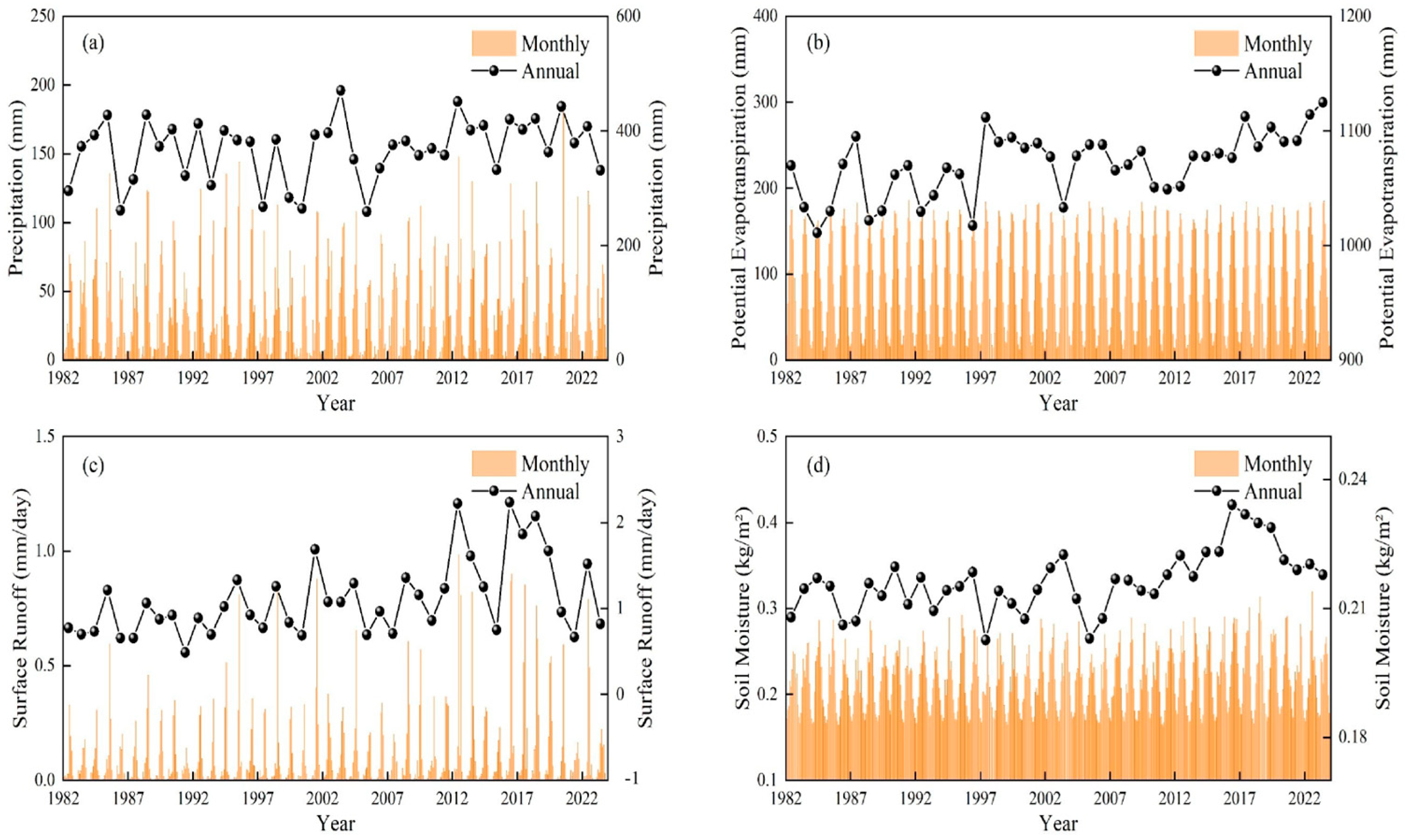
Figure 2 unveiled four discrete hydroclimatic regimes over the MUSL from 1982 to 2023. Precipitation culminated in July (72.6 mm) and reached its nadir in December (1.8 mm), thus delineating a pronounced monsoon-driven annual cycle. Potential evapotranspiration exhibited a consistent seasonal rhythm accompanied by interannual stability. Surface runoff demonstrated intermittent surge events concentrated in summer. Soil moisture alone manifested a statistically significant long-term upward trajectory, increasing by approximately 0.0007 kg·m⁻² per year. It further exhibited a typical monsoon-driven annual cycle punctuated by substantial intra-annual variations. Annual precipitation displayed a modest positive tendency (~0.68 mm/year). From 2012 onward, high-precipitation years recurred frequently, exceeding 400 mm on several occasions. This indicated that the regional climate had entered a comparatively pluvial phase. Potential evapotranspiration showed a stable annual pattern, with elevated values in May–June (monthly average >150 mm). Low values clustered in December–January (~18 mm). Its interannual variability remained marginal (stable average ~1070 mm). It exhibited a gradual ascending trend (~0.24 mm/year), which was consistent with augmented evaporative forcing under global warming. Surface runoff occurred predominantly from June to August, peaking in August. This sequence displayed a pronounced pulsed nature accompanied by strong interannual variation. Overall, a slight positive trend existed (~0.002 mm/year). Between 2016 and 2018, runoff extremes surpassing 2.0 mm ensued in succession, concomitant with the intense precipitation events during the same period. This underscored an amplified hydrological responsiveness to extreme precipitation. Surface soil moisture lagged behind precipitation by approximately one month, typically attaining its peak in August–September. The monthly average fluctuated between 0.26 and 0.27 kg·m⁻². This sequence manifested a significant long-term upward trend (~0.0007 kg·m⁻²/year), intimately linked to increased precipitation and the advantages derived from ecological restoration initiatives. It thus constituted critical hydrologic evidence for regional ecological improvement. Superimposed upon the annual cycle, longer-term fluctuation characteristics also existed in the sequence. Overall, during the past four decades, precipitation, potential evapotranspiration, surface runoff, and soil moisture in this region exhibited upward trends to varying extents. This reflected the MUSL climate’s transition toward warmer and wetter conditions, and the ecological environment demonstrated a trajectory of sustained amelioration.

4.1.2. Spatial Patterns

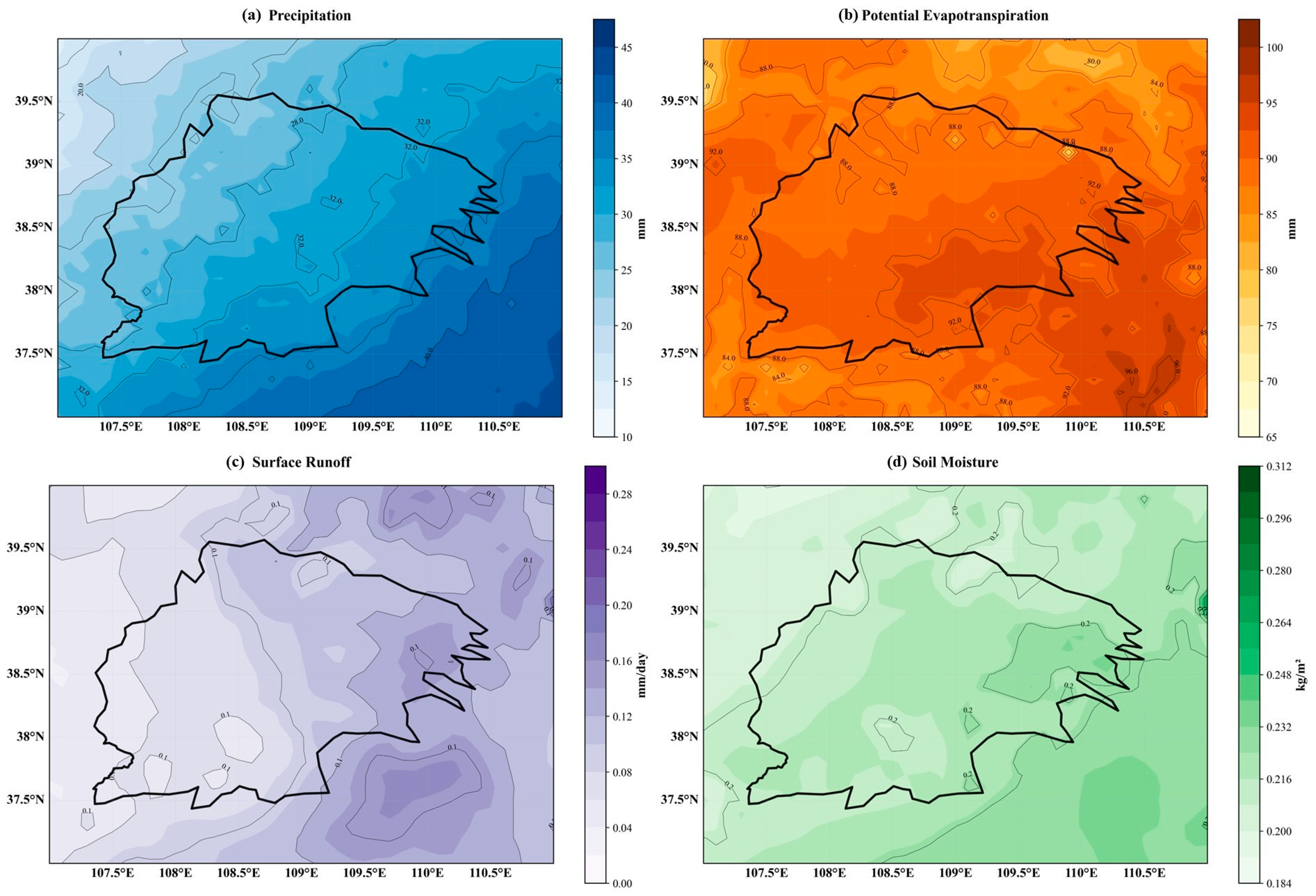
Figure 3 illustrated the spatial distributions of key hydroclimatic elements across the MUSL. Precipitation exhibited a gradient from southeast to northwest, decreasing from approximately 36 mm to 24 mm (standard deviation = 8.13 mm, coefficient of variation = 26.45%), reflecting the systematic influence of terrain and water vapor transport. Potential evapotranspiration was generally higher than precipitation and exhibited a south-to-north decline (92 mm to 88 mm; standard deviation = 3.31 mm), although the gradient was somewhat uneven, possibly attributable to local meteorological and surface factors. Surface runoff displayed an east–west contrast (0.05–0.15 mm/day; coefficient of variation = 38.52%), indicating strong sensitivity to underlying surface properties such as soil permeability and vegetation coverage. Soil moisture averaged 0.22 kg/m², with higher values in central areas (0.20–0.25 kg/m²) and a right-skewed distribution, consistent with vegetation restoration or local water accumulation. Collectively, these four elements revealed that hydroclimatic patterns across the MUSL were regulated by terrain, water vapor transport, and underlying surface properties, exhibiting both marked inter-variable differences and systematic spatial organization.

4.2. Statistical Detection of Trends and Abrupt Changes

4.2.1. Mann–Kendall Trend Test

Table 1. Results of the Mann–Kendall test for hydrometeorological elements.

Variable	p	z	Tau	β (10−3)
PRE	0.3946	0.8513	0.0254	2.956
PET	0.4970	0.6792	0.0203	8.111
SR	0.1097	1.5996	0.0477	0.006
SM	0.0008	3.3596	0.1002	0.025

revealed markedly divergent trend signatures among the four hydroclimatic variables. The p-values of precipitation and evapotranspiration were both greater than 0.05. They failed to pass the significance test. This indicated that no significant upward or downward trend was detected during the study period. The p-value of surface runoff was 0.1097. It did not reach the 0.05 significance level. However, its Tau statistic was 0.0477. This reflected a certain increasing tendency of surface runoff. Soil moisture showed an extremely significant upward trend. Its p-value was 0.0008 and the Tau value was 0.1002. The β slope was 0.025 × 10⁻³. This indicated that the moistening trend of soil moisture was statistically robust. Its change direction was consistent and continuous. Overall, only soil moisture showed a statistically significant upward trend at the 0.05 level. The other variables had certain changing tendencies, but none passed the significance test. This reflected that the hydroclimatic system of this region during the study period was mainly characterized by soil moisture increase.

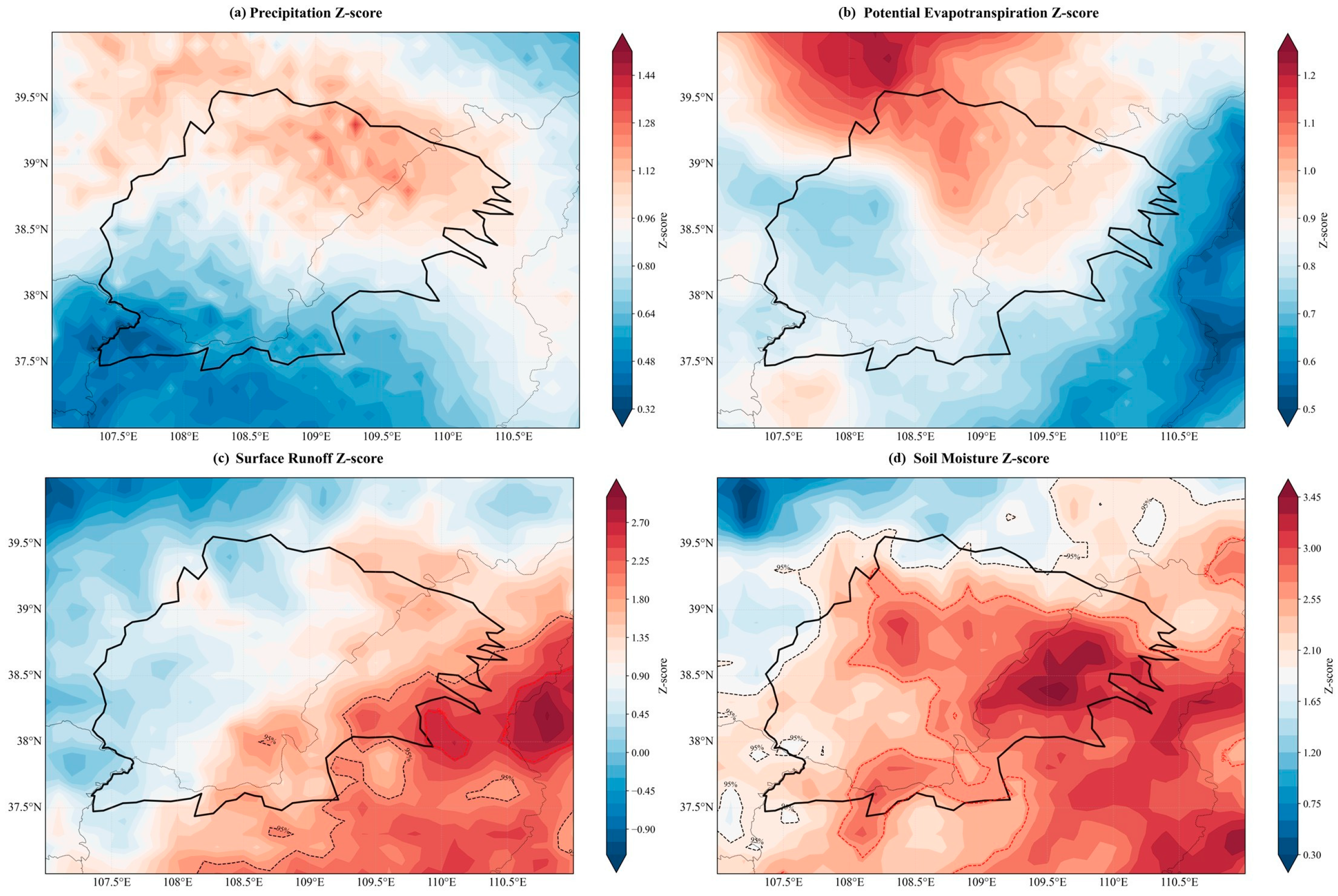
The spatial distribution of Z values was presented in Figure 4. Z values displayed distinct trend characteristics and spatial heterogeneity (Table 1). Precipitation Z values decreased from north to south. Z values remained below 1.5 across the entire area, with a relatively regular gradient. This gradient did not reach statistical significance, despite spatial differences. Potential evapotranspiration Z values remained below 1.3, with high values in the northern central and peripheral regions. Z values decreased toward the south and east–west flanks (east side slightly higher than north). The overall gradient was evident but did not reach significance. Runoff Z values spanned a wide range (−0.9 to 2.7). High values were concentrated in the southeast, decreasing toward the northwest. Some areas passed the 95% significance test, and a total of 24.35% of the pixels showed a significant increasing trend. This reflected strong spatial differentiation in regional runoff changes. Soil moisture Z values exceeded the 99% significance threshold across the entire area, with a relatively irregular spatial distribution. 73.15% of pixels showed a significant increasing trend. This confirmed an extremely significant moistening trend across the study area. Collectively, soil moisture emerged as the sole variable with a statistically robust directional trend, indicating that the regional hydrological system was dominated by a soil-moisture-led wetting process during the study period. Quantitatively, the proportion of pixels with a significant increasing trend (p < 0.05) was 0% for precipitation, 0% for potential evapotranspiration, 24.35% for surface runoff, and 73.15% for soil moisture, confirming that soil moisture greening was the most spatially widespread significant change.

4.2.2. Pettitt Test for Abrupt Change Points

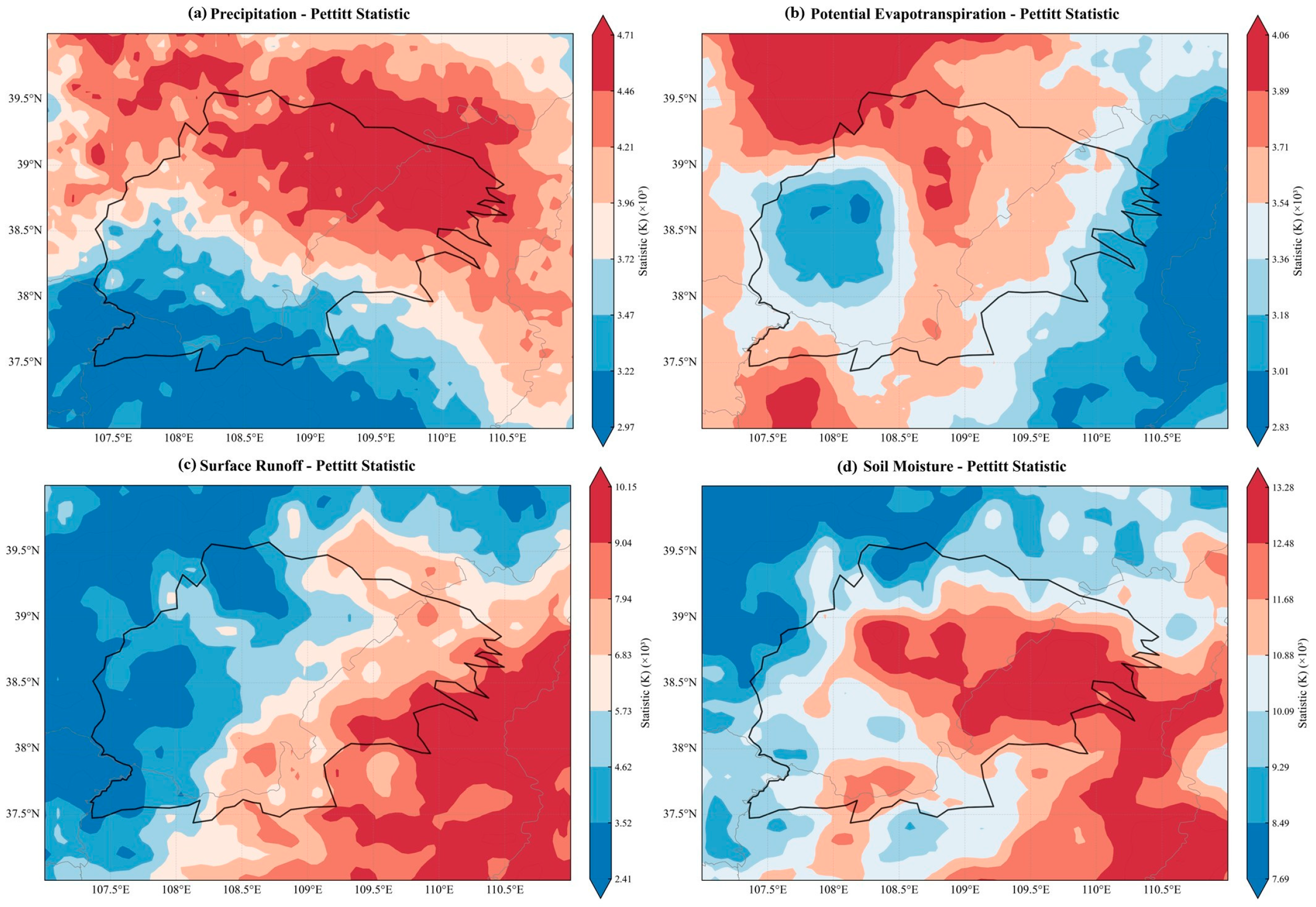
The Pettitt test results (

Table 2. Results of Pettitt test for environmental factors.

Variable	Statistic	p	Change Point	Significant Ratio (%)
PRE	3919	0.904	1 July 2001	0
PET	3454	0.992	1 April 1997	0
SR	5986	0.523	1 June 2001	15
SM	10,605	0.044	1 May 2011	82

) revealed divergent abrupt-change characteristics among the four hydro-meteorological variables. Precipitation (p = 0.904, mutation in July 2001) and potential evapotranspiration (p = 0.992, mutation in April 1997) both did not attain significance at the regional scale, with no detectable significant mutation pixels. Surface runoff (p = 0.523, mutation in June 2001) also showed no regional-scale shift, although approximately 15% of pixels displayed local mutations. In contrast, soil moisture (p = 0.044, mutation in May 2011) underwent a significant global abrupt change, with 82% of pixels confirming a spatially coherent moistening transition.

From the perspective of spatial distribution characteristics (Figure 5), the distribution patterns of the K values of each variable further confirmed the aforementioned trend. The K value of precipitation exhibited a north-high and south-low gradient. The K value of evapotranspiration exhibited a radial pattern with lower values in the west and higher values in the east. The K value of runoff was significantly higher in the southeast region, whereas the K value of soil moisture exhibited a high-value zone centered on the middle and eastern regions. Overall, only the soil moisture showed a statistically significant abrupt change at the regional scale, while the changes in the other variables were relatively stable. In summary, among the four indicators, namely precipitation, evapotranspiration, surface runoff, and soil moisture, only the soil moisture underwent a highly significant global abrupt change. The other indicators might have local variations, but overall they did not show systematic abrupt changes. This indicated that the dominant signal of the dry–wet changes in the MUSL during the study period was mainly manifested as a significant turning point in soil moisture and widespread moisture increase, which might reflect the response characteristics of the regional ecological hydrological process to climate change and human activities. The pixel-wise significant mutation ratios were 0% for precipitation, 0% for potential evapotranspiration, 15% for surface runoff, and 82% for soil moisture, indicating that only soil moisture experienced a spatially coherent abrupt change.

4.3. Periodic and Persistent Characteristics

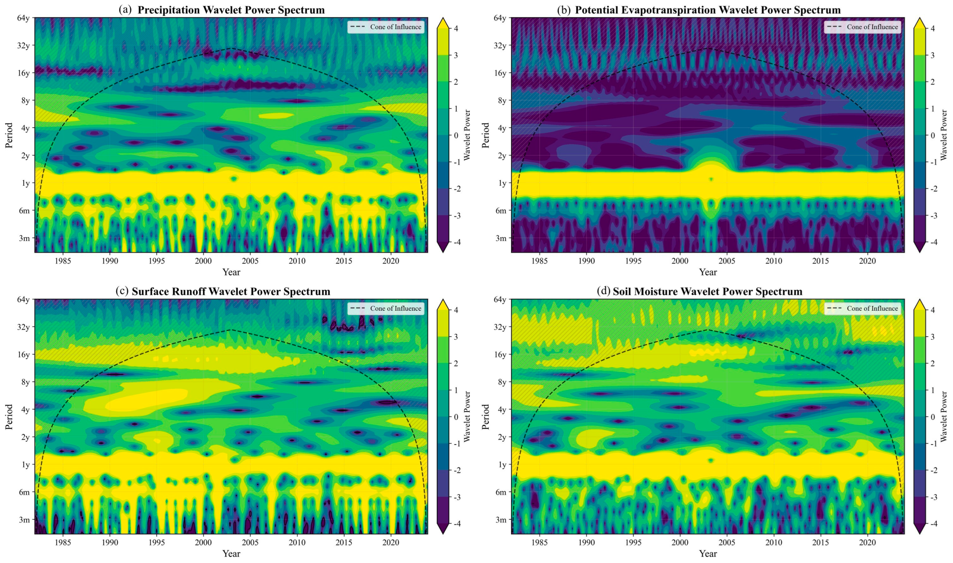
4.3.1. Wavelet-Based Periodicity

Wavelet analysis revealed multi-scale periodic oscillations across all variables from 1982 to 2024 (Figure 6). All variables exhibited a dominant power peak at the ~0.97-year seasonal cycle, with weaker secondary peaks at 1.04–1.12 years indicating modest interannual variation. However, the statistical significance of these cycles differed markedly. Precipitation and potential evapotranspiration did not pass the 95% confidence test; despite relatively high annual-cycle power, their significant wavelet area ratios and average power at the 2–8-year scale remained low, resulting in weak reliability of the periodic signals. In contrast, surface runoff and soil moisture displayed statistically robust periodic structures with large-scale continuous significant regions. Their 2–8-year average power substantially exceeded that of the meteorological variables and fell entirely within the significant domain, confirming statistically reliable interannual variations.

The strongest power cycle and the strongest significant cycle differed across variables. For precipitation and potential evapotranspiration, the dominant cycle represented only a power ranking without statistical significance. In contrast, surface runoff and soil moisture displayed a strongest significant cycle of approximately 0.17 years (~2 months), indicating that the most statistically reliable periodic disturbance occurred at the intraseasonal scale. Overall, oscillation energy alternated between seasonal (~0.85–0.97 years) and interannual (~1.04–1.12 years) cycles, reflecting the joint influence of multi-scale oscillation modes. Only hydrological variables exhibited definite statistical significance. Precipitation and potential evapotranspiration exhibited periodic fluctuations, yet their periodic signals failed to attain statistical significance; by contrast, surface runoff and soil moisture manifested statistically significant periodic structures spanning intraseasonal to interannual scales, which implied more stable and discernible oscillatory patterns and attested to the regulatory role of underlying surface and ecological processes on the hydrological cycle.

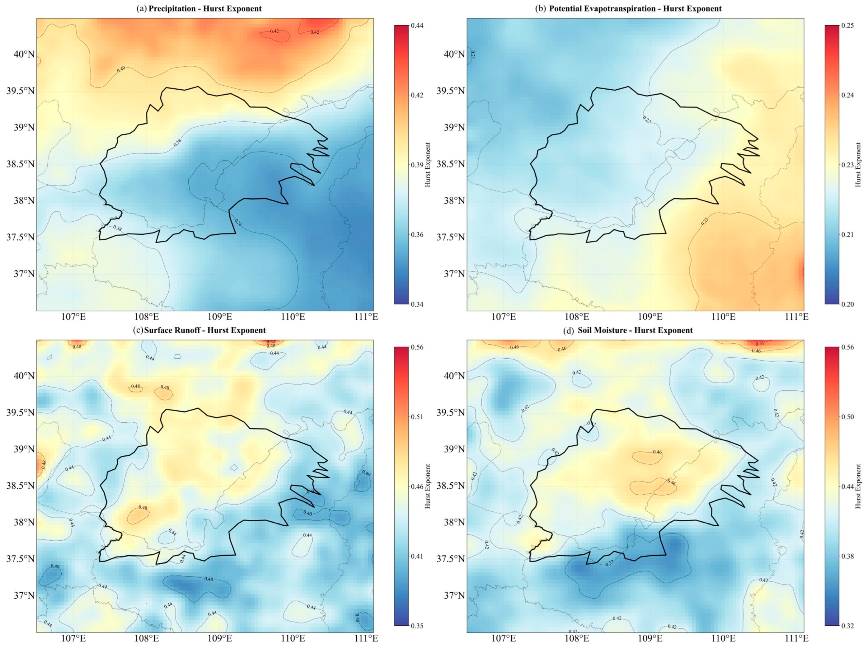
4.3.2. Hurst Index and Future Trend Persistence

Hurst index analysis revealed marked inter-variable differences in long-range persistence (Figure 7). Precipitation displayed uniform anti-persistence (mean H = 0.379, standard deviation = 0.020, 84.2% strong and 15.8% moderate anti-persistence), with a north-to-south decreasing gradient. Potential evapotranspiration exhibited the most intense and spatially uniform anti-persistence (mean H = 0.222, standard deviation = 0.004, coefficient of variation = 0.018; 100% extremely strong anti-persistence). Hydrological variables generally tended toward a more stochastic state with greater spatial complexity. Surface runoff showed the highest mean H (0.436, standard deviation = 0.022, range = 0.225) and the most complex persistence status: 68.1% moderate anti-persistence, 26.2% weak anti-persistence, with minor proportions of random and weak persistence states totaling approximately 5.7%. Soil moisture presented a similarly complex profile (mean H = 0.414, standard deviation = 0.026), with 63.8% moderate anti-persistence, 28.7% strong anti-persistence, 5.7% weak anti-persistence, and small proportions of random (1.3%) and weak persistence (0.5%). Collectively, meteorological elements exhibited stronger anti-persistence and lower spatial variability, whereas hydrological elements exhibited weaker persistence and higher spatial heterogeneity, suggesting greater future unpredictability in the latter.

4.4. Important Predictors Identified by LightGBM

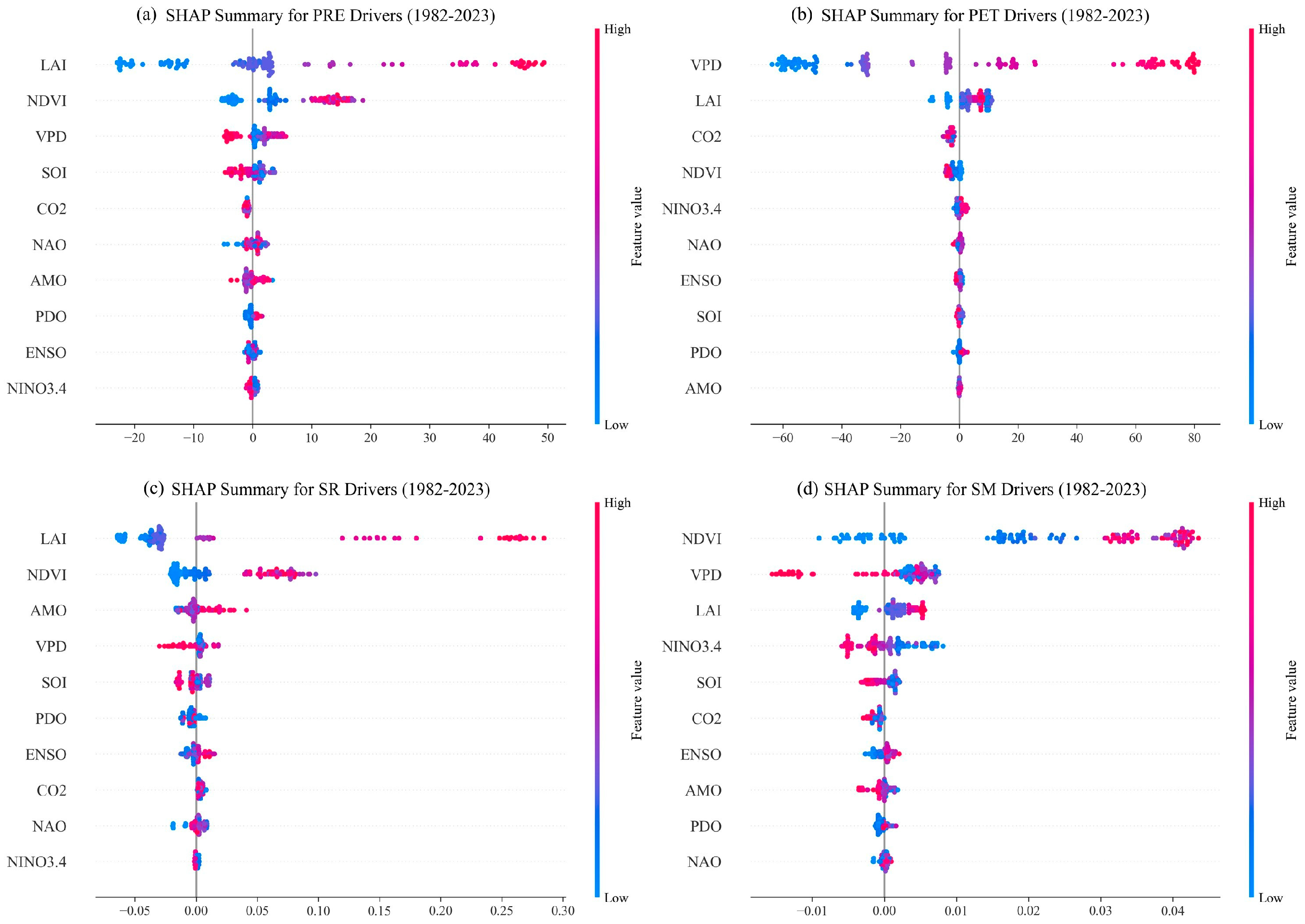
The predictive performance of the LightGBM model was first assessed under the time-series cross-validation framework described in Section 3.4. The model achieved acceptable cross-validated predictive skill across all four target variables. The performance metrics (R², RMSE, and MAE) and their inter-fold standard deviations indicated robust and stable prediction accuracy. These validation results supported the reliability of the subsequent SHAP-based importance rankings. Based on the LightGBM model and SHAP analysis, this study identified the most important predictors (statistically associated factors) and their relative importance scores for the four key variables: precipitation, potential evapotranspiration, surface runoff, and soil moisture (Figure 8). The results showed that the dominant driving mechanisms of different variables were significantly different. The temporal and spatial variation of precipitation was strongly associated with local vegetation dynamics and atmospheric conditions. The SHAP contributions of the leaf area index and the normalized vegetation index were the highest, and both were strongly positively correlated with precipitation. This indicated that regional vegetation coverage, through transpiration and changes in surface properties, might exert an important feedback on local convection. The water vapor pressure difference, as an indicator of atmospheric aridity, contributed secondarily, highlighting the direct constraint of atmospheric humidity on precipitation formation. In contrast, the contributions of various large-scale climate indices were weak and the correlations were not significant. This result indicated that precipitation in the study area showed the strongest statistical association with local land–atmosphere interaction processes on a monthly scale. The statistical pattern of potential evapotranspiration was completely different, and its variation was most strongly associated with a single physical variable. The SHAP contribution of the water vapor pressure difference was extremely high, with a correlation coefficient of 0.97 with potential evapotranspiration. This confirmed that atmospheric evaporation demand was the most important predictor (statistically) for its temporal and spatial variations. The contribution of the leaf area index ranked second, demonstrating the biological and physical control of vegetation. It should be noted that LightGBM and SHAP quantify statistical associations and predictive importance, which do not necessarily imply causal relationships. Causal interpretations require additional physical mechanism analysis or experimental validation.

Surface runoff variation was primarily associated with underlying surface properties. The leaf area index and normalized vegetation index contributed most strongly. Their moderate positive correlation with runoff indicated a linkage between vegetation condition and runoff generation, likely mediated by effects on infiltration and surface resistance. Vapor pressure deficit contributed relatively little but still indirectly affected runoff by influencing initial soil moisture. Overall, the surface runoff model exhibited relatively limited explanatory power, suggesting that other key local factors might have controlled the runoff process. Soil moisture changes further confirmed the core driving role of underlying surface properties. The normalized vegetation index exhibited the highest contribution and emerged as the most sensitive driver; its strong correlation underscored the dual regulation of vegetation on soil water consumption and retention. The leaf area index and vapor pressure deficit contributed secondarily. As with precipitation and potential evapotranspiration, the concurrent direct influence of all large-scale climate indices on soil moisture was not significant.

A comprehensive comparison revealed a clear dichotomy in the monthly-scale drivers. Local biogeochemical processes, particularly vegetation dynamics, dominated the prediction of precipitation, runoff, and soil moisture. In contrast, potential evapotranspiration was controlled almost exclusively by atmospheric evaporative demand. Large-scale climate indices contributed minimally to all four variables, suggesting that local land–atmosphere interactions rather than remote teleconnections governed the hydroclimatic variability of the MUSL. This highlighted the extreme importance of accurately representing vegetation dynamics in regional hydrological simulations. Additionally, the analysis results revealed differences in the statistical associations of different components in the hydrological cycle: potential evapotranspiration showed the strongest statistical association with energy-related variables (i.e., atmospheric evaporation demand), whereas precipitation, runoff, and soil moisture were more strongly associated with water availability and underlying surface processes. This systematic difference profoundly reflected the unique response modes of each component of the terrestrial hydrological cycle to climate and environmental changes. In terms of relative importance (normalized SHAP values), the top two predictors for precipitation (LAI and NDVI) together accounted for approximately 68% of the total predictive importance; for potential evapotranspiration, VPD alone contributed over 85%; for surface runoff, LAI and NDVI contributed approximately 55%; for soil moisture, NDVI contributed approximately 42%. These quantitative breakdowns highlighted the dominant role of vegetation dynamics and atmospheric demand.

5. Discussion

5.1. Interpretation of Spatiotemporal Patterns

The spatiotemporal analysis yielded three salient features that characterized the hydroclimatic evolution of the MUSL from 1982 to 2023. Overall, the region exhibited a warming–wetting tendency, but the response characteristics of different elements were significantly different [20]. Notably, only soil moisture displayed a statistically robust long-term increase, while the upward tendencies of precipitation, potential evapotranspiration, and surface runoff all failed to reach significance—suggesting that the regional hydroclimatic shift was not uniformly expressed across the water cycle. In contrast to previous studies that reported significant precipitation increases over longer periods, our study detected no statistically significant trend for precipitation (p = 0.3946) or potential evapotranspiration (p = 0.4970) during 1982–2023, suggesting that trend significance might be sensitive to the study period. Among them, soil moisture showed a highly significant long-term increase in humidity, while the upward trends of precipitation and potential evapotranspiration did not pass the statistical significance test. This phenomenon suggested that, in addition to climate background changes, large-scale ecological restoration projects might have played a role in enhancing soil moisture retention capacity by improving surface conditions, potentially amplifying the moistening signal. However, because soil moisture was the only variable with a statistically significant trend, this interpretation remained speculative and required further investigation using process-based models or controlled experiments [48]. In terms of spatial distribution, each element exhibited a systematic pattern regulated by multiple factors. These features were controlled by large-scale atmospheric circulation (precipitation gradient), latitudinal energy distribution (PET), and local surface properties (runoff). The soil moisture showed an uneven distribution pattern, with higher values in the central area and lower values in the surrounding areas. Human activities (such as vegetation restoration) may have had an impact on the local hydrological processes, although this causal relationship cannot be directly determined from the statistical evidence alone [49]. Compared with previous correlation-based analyses, our SHAP approach identified NDVI as the most important predictor for soil moisture, demonstrating the added value of machine learning for attribution. This finding suggested that vegetation greening—likely associated with ecological restoration projects—may have enhanced soil moisture retention in the central area, which was consistent with the observed patchy distribution of higher soil moisture values.

5.2. Dynamics of Trends and Periodicity

This study systematically investigated the periodic and persistence characteristics of the hydroclimatic system in the MUSL. Systematic differences existed in the intrinsic dynamic mechanisms of meteorological and hydrological elements. Hydrological elements responded more deterministically to intraseasonal forcing and displayed weaker long-term persistence than meteorological elements, rendering hydrological predictions inherently more uncertain and spatially variable. These differences confirmed that the response of the hydrological system to climate-driven factors was more complex and uncertain. For meteorological variables (H < 0.5), anti-persistence implied that historical trends were likely to reverse, indicating low predictability and potential climate regime shifts. For hydrological variables (H ≈ 0.5), near-random behavior meant future changes were largely unpredictable and the system was highly sensitive to disturbances, reducing stability. This study integrated wavelet analysis, the Hurst index, and LightGBM to reveal an intrinsic connection between the multi-scale oscillation modes identified by wavelet analysis and the long-term memory quantified by the Hurst index. Furthermore, LightGBM captured the key nonlinear factors driving these mode transitions, revealing the essence of hydroclimatology more comprehensively than any single method.

Before interpreting the CMIP6 projections, the relationship between the Hurst analysis and the CMIP6 results was clarified. The Hurst index inferred future trend persistence or reversal solely based on historical statistics, without considering emission scenarios. In contrast, CMIP6 projected future changes under specific scenarios using physically based models. The two approaches serve complementary roles: Hurst provides a data-driven baseline, while CMIP6 offers scenario-dependent projections. For example, the Hurst analysis indicated strong anti-persistence for precipitation and PET, suggesting a reversal of historical trends, whereas CMIP6 under high-emission scenarios showed persistent warming and moistening. This apparent contradiction highlighted the inherent uncertainty in future projections and the value of multi-method cross-validation. Thus, the two analyses were to be viewed as complementary rather than conflicting.

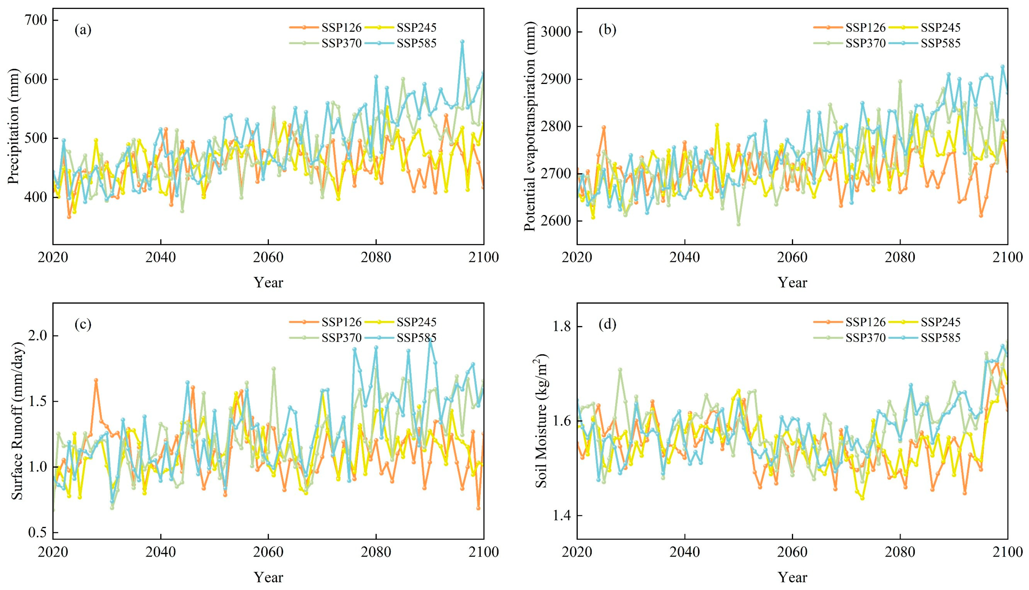
CMIP6 multi-model projections (Figure 9) indicated a concurrent water–heat increase under future emission scenarios [50]. The trends in precipitation, potential evapotranspiration, surface runoff, and soil moisture under different emission scenarios were directly derived from the raw multi-model ensemble mean (Section 2.2). The statements regarding evapotranspiration-driven drought risk intensification, cascading hydrological responses, and soil moisture sustainability uncertainty at the end of the high-emission period represented inferences from historical statistical relationships rather than direct CMIP6 outputs. Unlike national-scale compound-extreme projections, our results specifically quantified that under the high-emission scenario, potential evapotranspiration outpaced precipitation growth. This differential amplification might partially offset water gains and elevate regional drought stress at certain stages [51], consistent with previous semi-arid projections reporting stronger evapotranspiration increases under high-emission conditions. Under the low-emission scenario, synchronized water–heat growth yielded more moderate water-balance shifts. High-temperature-driven evapotranspiration intensification amplified drought-stress potential under the high-emission trajectory. The response of hydrological processes to climate forcing exhibited a cascading effect: precipitation changes propagated to runoff and soil moisture through altered infiltration and evaporation pathways, magnifying the net water deficit. Consequently, surface runoff variability increased under the high-emission scenario, implying a higher likelihood of extreme hydrological events. Soil moisture displayed a lagged and integrated response, generally following a wetting trend driven by precipitation increases, yet the sustainability of this gain remained uncertain by the end of the high-emission period [52]. The continuous intensification of evapotranspiration might gradually erode the long-term accumulation of soil moisture in the future. These projections were inherently uncertain, particularly for soil moisture trends under high-emission scenarios. Nevertheless, soil moisture emerged as a key indicator of regional dry–wet conditions and ecological resilience.

Future drought risk management required a multi-dimensional assessment system, with both macro-scale climate forcing and micro-scale hydrological responses considered simultaneously, accounting for dual uncertainties. A comprehensive assessment framework should integrate composite drought indices, high-resolution hydrological models, and core soil moisture monitoring. Such a system will help better cope with the increasingly complex climate risk challenges.

5.3. Limitations and Future Research Directions

Although this study employed advanced datasets and methods, it to some extent revealed the patterns of regional environmental evolution. However, it still had several limitations, which also highlighted directions for further research. At the data level, although the grid data used in this study had been processed and possessed a relatively high resolution, its spatial representativeness in complex terrain areas might still be inferior to in situ observations. Meanwhile, the interpolation, standardization, and other operations during data preprocessing might introduce uncertainties, thereby affecting the accuracy of subsequent analyses. Moreover, the hydrometeorological elements selected in this study were core hydrological and climatic variables, but the regional climate system was governed by multiple layers and scales of processes. The current indicator system had not fully incorporated the influence of key processes such as snow dynamics, groundwater level changes, and vegetation physiological responses.

In addition, uncertainties associated with the multi-source datasets themselves were not quantitatively assessed. The gridded precipitation, potential evapotranspiration, runoff, soil moisture, and vegetation index datasets used in this study were derived from satellite retrievals, reanalysis, or spatial interpolation. Each product carries inherent uncertainties due to measurement errors, spatial resolution, temporal gaps, and algorithmic assumptions. Although quality control was performed and all data were resampled to a uniform 0.1° resolution with missing values filled by interpolation, the propagation of these uncertainties through the subsequent statistical and machine learning analyses was not quantified. Future work would need to adopt ensemble datasets or error propagation techniques to better constrain the impact of input data uncertainties on the final conclusions. Furthermore, simply resampling all datasets to a common 0.1° grid and applying interpolation did not eliminate the intrinsic differences in data generation mechanisms, error structures, and spatiotemporal representativeness among the various products. This comparability issue remains a limitation of the current data fusion approach and may affect the robustness of the subsequent analyses. Future research would need to develop more rigorous harmonization frameworks to better account for these discrepancies.

Another limitation concerns the CMIP6 future projections presented in this study. These projections were subject to multiple sources of uncertainty, including emission scenarios, model structural differences, and internal climate variability. While a multi-model ensemble (MME) approach was used to reduce single-model bias, the ensemble spread was not explicitly quantified. Moreover, the downscaling procedure may have introduced additional uncertainties. Furthermore, the analysis relied on raw CMIP6 outputs without prior systematic bias correction, which may have left uncorrected systematic offsets in the projected magnitudes. Therefore, the future trends shown in Figure 9 should be interpreted as indicative directions of change rather than precise forecasts. A more rigorous uncertainty quantification (e.g., using confidence intervals derived from the model spread or probabilistic projections) was recommended for future research. In addition, neither a systematic historical performance assessment of the selected CMIP6 models nor formal bias correction was performed in this study. Specifically, direct comparisons of raw CMIP6 outputs against observational data during the overlapping historical period (1982–2014) were not conducted, and consequently the manuscript does not include bias-corrected results or quantitative validation metrics (e.g., correlation coefficients, RMSE, Taylor diagrams). This limits the quantitative validation of the CMIP6 ensemble against regional observations and represents a significant methodological gap. Future work should prioritize such an evaluation—including explicit intercomparison of raw outputs, corrected results, and observational benchmarks—alongside formal bias correction procedures to better constrain projection uncertainties.

At the method and model level, this study also had certain limitations. Firstly, the assessment of future trends was mainly based on historical statistical laws and the correlation between elements, and had not been coupled with hydrological models or Earth system models with clear physical mechanisms. Therefore, there were deficiencies in simulating the dynamic feedback processes under the dual influence of climate change and human activities. Secondly, although machine learning methods such as LightGBM can effectively identify key drivers, their limitations in interpretability restrict our understanding of the nonlinear interaction and cascading effects among factors. Furthermore, although the LightGBM model was rigorously validated through time-series cross-validation and achieved acceptable predictive performance the SHAP-based feature importance analysis quantified statistical associations rather than causal inferences. In addition, extensive hyperparameter tuning and robustness quantification (e.g., multiple random seeds or repeated cross-validation) were not performed for the LightGBM model, which limited the reproducibility of the attribution results. Future work would need to incorporate more physical variables and process-based models to reduce this uncertainty.

To deepen understanding, future work should promote the organic integration of process mechanism models and data-driven models, systematically reveal the contribution and interaction mechanisms of each driving factor, and enhance the physical transparency and reliability of the research results. Future research should also focus on developing dynamic fusion and assimilation technologies for multi-source heterogeneous data, and constructing more reliable long-term, high-consistency datasets, so as to more comprehensively characterize the complex state of the regional hydrological and climatic system.

6. Conclusions

This study, based on multi-source data and various statistical methods, systematically revealed the temporal and spatial evolution patterns, future trend characteristics, and key driving mechanisms of hydroclimatic elements in the MUSL from 1982 to 2023. The main conclusions are as follows:

Over the past four decades, all four hydroclimatic variables (precipitation, potential evapotranspiration, surface runoff, and soil moisture) exhibited a positive trend, suggesting a shift toward warmer and wetter conditions. However, this tendency was statistically significant only for soil moisture (p < 0.05), which also showed a clear global abrupt change point. The positive trends of precipitation, potential evapotranspiration, and surface runoff did not attain the 0.05 significance level. Therefore, the statistically significant moistening signal was primarily reflected in soil moisture, while the other variables showed only non-significant upward tendencies. This confirmed that the continuous increase in soil moisture was an important hydrological indicator consistent with local ecosystem recovery, although other factors (such as land use change and vegetation restoration) might have also contributed, and the observed trend in soil moisture alone did not constitute conclusive evidence of a regional climate regime shift. The spatial patterns of each element were highly heterogeneous, reflecting the comprehensive regulation of terrain, water vapor transport, and underlying surface properties.

Systematic differences existed in the dynamic mechanisms of hydrological and meteorological elements. The periodic fluctuations of meteorological elements were not significant, and future changes displayed a strong anti-continuity. In contrast, hydrological elements displayed significant periodic oscillations on seasonal to interannual scales. Their future changes approached a random state, with greater spatial heterogeneity and more complex responses. This difference highlighted the regulatory role of underlying surface processes on the hydrological system.

Monthly-scale variations showed strong statistical associations with local surface processes. Vegetation dynamics were identified as the most important predictors for precipitation, runoff, and soil moisture, which was consistent with the hypothesis that ecological restoration projects may influence the local hydrological cycle. However, direct causal attribution was not possible from the machine learning analysis alone. Changes in potential evapotranspiration were most strongly associated with atmospheric evaporation demand. The regional hydrological cycle exhibited a differentiated feature of energy-driven and water-process regulation.

This study had important implications for regional climate management. Although soil moisture increased throughout the historical period, persistent drought risk remained possible under future high-emission scenarios. Given the uncertainty and sensitivity of hydrological processes, a multi-dimensional climate risk management system was needed. A comprehensive early warning framework integrating multi-scale monitoring, high-resolution models, and vegetation feedback mechanisms should be developed. The crucial role of underlying surface management in enhancing regional ecological resilience warrants emphasis.

References

1. Keat, W.J.; Kendon, E.J.; Bohnenstengel, S.I. Climate change over UK cities: The urban influence on extreme temperatures in the UK climate projections. Clim. Dyn. 2021, 57, 3583–3597. [Google Scholar] [CrossRef]
2. Blunden, J.; Boyer, T. State of the Climate in 2021. Bull. Am. Meteorol. Soc. 2022, 103, S1–S465. [Google Scholar] [CrossRef]
3. Liu, Q.; Fu, C.; Xu, Z.; Ding, A. Global warming intensifies extreme day-to-day temperature changes in mid–low latitudes. Nat. Clim. Change 2025, 16, 69–76. [Google Scholar] [CrossRef]
4. Du, J.; Zhou, L.; Yu, X.; Ding, Y.; Zhang, Y.; Wu, L.; Ao, T. Understanding precipitation concentration changes, driving factors, and responses to global warming across mainland China. J. Hydrol. 2024, 645. [Google Scholar] [CrossRef]
5. Kim, D.; Lee, S.; Cho, S.; Kim, D.; Choi, M. Evaluating rainfall estimates derived from soil moisture using soil hydraulic properties over the Korean Peninsula. J. Hydrol. 2025, 663, 134267. [Google Scholar] [CrossRef]
6. Wang, L.; Dai, X.; Wang, G.; Yinglan, A.; Miao, C.; Xue, B.; Wang, Y.; Zhu, Y. Establishment of a slope-scale innovated rainfall-runoff model by combining infiltration equation and motion wave equation for watershed flash flood risk prediction. J. Hydrol. 2025, 652, 132700. [Google Scholar] [CrossRef]
7. Tang, R.; Qian, L. Multi-indicator comparison in characterizing spatiotemporal patterns of water disasters and corresponding agricultural applications in the Middle-and-lower Yangtze River. Agric. Water Manag. 2025, 321, 109878. [Google Scholar] [CrossRef]
8. Yang, G.-Y.; Guo, L.-L.; Feng, Y.-H.; Chu, Y.; Li, T.-W.; Xu, H.-T.; Zheng, H.; He, B. Widespread loss of ecosystem resilience in response of 1.5 and 2 °C global warming. Adv. Clim. Change Res. 2025, 17, 117–127. [Google Scholar] [CrossRef]
9. Shu, Z.; Jin, J.; Zhang, J.; Wang, G.; Lian, Y.; Liu, Y.; Bao, Z.; Guan, T.; He, R.; Liu, C.; et al. 1.5 °C and 2.0 °C of global warming intensifies the hydrological extremes in China. J. Hydrol. 2024, 635. [Google Scholar] [CrossRef]
10. IPCC. Climate Change 2021: The Physical Science Basis. Working Group I Contribution to the IPCC Sixth Assessment Report; Cambridge University Press: Cambridge, UK; New York, NY, USA, 2021. [Google Scholar] [CrossRef]
11. Su, B.; Huang, J.; Fischer, T.; Wang, Y.; Kundzewicz, Z.W.; Zhai, J.; Sun, H.; Wang, A.; Zeng, X.; Wang, G.; et al. Drought losses in China might double between the 1.5 °C and 2.0 °C warming. Proc. Natl. Acad. Sci. USA 2018, 115, 10600–10605. [Google Scholar] [CrossRef] [PubMed]
12. Chen, X.; Zhang, Y. Impacts of climate, phenology, elevation and their interactions on the net primary productivity of vegetation in Yunnan, China under global warming. Ecol. Indic. 2023, 154, 110533. [Google Scholar] [CrossRef]
13. CMA. Blue Book on Climate Change in China (2023); Science Press: Beijing, China, 2023. [Google Scholar]
14. Liu, L.; Gou, X.; Wang, X.; Yang, M.; Qie, L.; Pang, G.; Wei, S.; Zhang, F.; Li, Y.; Wang, Q.; et al. Relationship between extreme climate and vegetation in arid and semi-arid mountains in China: A case study of the Qilian Mountains. Agric. For. Meteorol. 2024, 348, 109938. [Google Scholar] [CrossRef]
15. Mao, S.; Lv, J.; Li, M.; Li, L.; Xue, J. Trade-off and driving factors of water-energy-food nexus in Mu Us sandy land, China. J. Clean. Prod. 2024, 434, 139852. [Google Scholar] [CrossRef]
16. Xu, Z.; Liang, W.; Lei, J.; Wu, Y.; Wang, Z. Monitoring and assessment of desertification reversal in ecologically fragile areas: A case study of the Mu Us Sandy Land. J. Environ. Manag. 2025, 373, 123695. [Google Scholar] [CrossRef]
17. Hirko, D.B.; Du Plessis, J.A.; Bosman, A. Using machine learning and satellite data to analyse climate change in the Upper Awash Sub-basin, Ethiopia. Phys. Chem. Earth Parts A/B/C 2025, 141, 104137. [Google Scholar] [CrossRef]
18. Wang, X.; Song, C.; Yang, T.; Gu, H.; Liu, G.; Zhan, P. How well do the CMIP6 climate models capture terrestrial water storage variations in data-scarce basins originating from the high mountains of Asia? J. Hydrol. 2025, 661, 133677. [Google Scholar] [CrossRef]
19. Lee, T.; Ouarda, T.B.M.J. Climate teleconnection-driven stochastic simulation for future water-related risk management. J. Hydrol. 2025, 662, 133834. [Google Scholar] [CrossRef]
20. Liang, L.E.; Chao, Y.; Wang, X.; Li, J.; Ma, P. Seasonal climate change characteristics of the Mu Us Sandy Land based on long time scale. Environ. Monit. Assess. 2025, 197, 771. [Google Scholar] [CrossRef]
21. Liu, J.-Y.; Nie, H.-F.; Xu, L.; Xiao, C.-L.; Li, W.; Yuan, G.-L.; Huang, Y.-P.; Ji, X.-Y.; Li, T.-Q. Assessment of ecological geological vulnerability in Mu Us Sandy Land based on GIS and suggestions of ecological protection and restoration. China Geol. 2025, 8, 117–140. [Google Scholar] [CrossRef]
22. Zhang, Z.; Wang, S.; Han, L.; Pan, K.; Liu, X.; Wang, R.; Dong, Z. Farmland wind erosion in the Mu Us Desert, China. Soil Tillage Res. 2026, 255, 106788. [Google Scholar] [CrossRef]
23. Liao, J.; Peng, F.; Kang, W.; Chen, X.; Sun, J.; Chen, B.; Xia, Y.; Du, H.; Li, S.; Song, X.; et al. No increase of soil wind erosion with the establishment of center pivot irrigation system in Mu-Us sandy land. Sci. Total Environ. 2024, 939, 173558. [Google Scholar] [CrossRef]
24. Qu, Q.; Wang, Z.; Xu, H.; Liu, R.; Wang, M.; Xue, S. Sand dune fixation enhances the contribution of microbial necromass carbon to soil organic carbon: A case study of Mu Us Sandy Land in China. Appl. Soil Ecol. 2025, 209, 106011. [Google Scholar] [CrossRef]
25. Shouzhang, P. 1-km Monthly Precipitation Dataset for China (1901–2022); Copernicus Publications: Göttingen, Germany, 2020. [Google Scholar] [CrossRef]
26. Shouzhang, P. 1 km Monthly Potential Evapotranspiration Dataset in China (1901–2022); Copernicus Publications: Göttingen, Germany, 2022. [Google Scholar] [CrossRef]
27. Ma, Y.; Ren, J.; Kang, S.; Niu, J.; Tong, L. Spatial-temporal dynamics of meteorological and agricultural drought in Northwest China: Propagation, drivers and prediction. J. Hydrol. 2025, 650, 132492. [Google Scholar] [CrossRef]
28. Li’e, L.; Xiaohan, W.; Yan, C.; Jiamin, L.; Yonghua, Z. Drought assessment and development trend in Mu Us Sandy Land based on standardized precipitation and potential evapotranspiration index. Clim. Serv. 2025, 39, 100588. [Google Scholar] [CrossRef]
29. Zhang, Q.; Miao, C.; Su, J.; Gou, J.; Hu, J.; Zhao, X.; Xu, Y. A new high-resolution multi-drought-index dataset for mainland China. Earth Syst. Sci. Data 2025, 17, 837–853. [Google Scholar] [CrossRef]
30. Li, H.; Cao, Y.; Xiao, J.; Yuan, Z.; Hao, Z.; Bai, X.; Wu, Y.; Liu, Y. A daily gap-free normalized difference vegetation index dataset from 1981 to 2023 in China. Sci. Data 2024, 11, 527. [Google Scholar] [CrossRef]
31. Cao, S.; Li, M.; Zhu, Z.; Wang, Z.; Zha, J.; Zhao, W.; Duanmu, Z.; Chen, J.; Zheng, Y.; Chen, Y.; et al. Spatiotemporally consistent global dataset of the GIMMS leaf area index (GIMMS LAI4g) from 1982 to 2020. Earth Syst. Sci. Data 2023, 15, 4877–4899. [Google Scholar] [CrossRef]
32. Lv, H.; Wang, Y.; Yan, D.; Peng, S.; Zheng, X. Quantifying the impacts of climate change and human activities on hydrological regime in Jinsha River, China. J. Hydrol. 2025, 662, 134008. [Google Scholar] [CrossRef]
33. Jamalzi, A.R.; Rahman, G.; Akhtar, F.; Ikram, Q.D.; Kwon, H.-H. Spatiotemporal assessment and trend analysis of meteorological drought in Afghanistan (1974–2023) using SPI and SPEI indices. J. Hydrol. Reg. Stud. 2025, 61, 102711. [Google Scholar] [CrossRef]
34. Solaimani, K.; Bararkhanpour Ahmadi, S. Evaluation of TerraClimate gridded data in investigating the changes of reference evapotranspiration in different climates of Iran. J. Hydrol. Reg. Stud. 2024, 52, 101678. [Google Scholar] [CrossRef]
35. Pettitt, A.N. A Non-Parametric Approach to the Change-Point Problem. J. R. Stat. Soc. Ser. C 1979, 28, 126–135. [Google Scholar] [CrossRef]
36. Rodríguez-Souilla, J.; Bottan, L.; Cellini, J.M.; Chaves, J.E.; Lencinas, M.V.; Roig, F.A.; Martínez Pastur, G. Climate thresholds and productivity shifts in mature Nothofagus pumilio height growth. For. Ecol. Manag. 2025, 596, 123055. [Google Scholar] [CrossRef]
37. Li, Y.; Zhang, T.; Zhao, Y.; Guo, Z.; Han, P.; Zhong, Q.; Liu, L.; Mao, S.; Wang, Y.; Li, D. Impact of climate change and vegetation greening on sediment transport in the Yarlung Tsangpo River. Catena 2025, 261, 109557. [Google Scholar] [CrossRef]
38. Ji, C.; Huang, Y.; Liu, J.; Wu, X.; Chen, L. Response characteristics of vegetation net primary production to cascade hydropower development and climate change in the dry-hot valleys of the Jinsha River. J. Hydrol. Reg. Stud. 2025, 62, 102880. [Google Scholar] [CrossRef]
39. Liu, Y.; Li, H.; Yang, Y.; Pang, X.; Niu, L. Enhancing machine learning runoff simulation via wavelet-based abnormality pattern recognition. J. Hydrol. 2025, 661, 133729. [Google Scholar] [CrossRef]
40. Tsai, J.-P.; Hsiao, C.-T. Spatiotemporal analysis of the groundwater head variation caused by natural stimuli using independent component analysis and continuous wavelet transform. J. Hydrol. 2020, 590, 125405. [Google Scholar] [CrossRef]
41. Chong, K.L.; Huang, Y.F.; Koo, C.H.; Najah Ahmed, A.; El-Shafie, A. Spatiotemporal variability analysis of standardized precipitation indexed droughts using wavelet transform. J. Hydrol. 2022, 605, 127299. [Google Scholar] [CrossRef]
42. Cheng, V.Y.S.; Saber, A.; Alberto Arnillas, C.; Javed, A.; Richards, A.; Arhonditsis, G.B. Effects of hydrological forcing on short- and long-term water level fluctuations in Lake Huron-Michigan: A continuous wavelet analysis. J. Hydrol. 2021, 603, 127164. [Google Scholar] [CrossRef]
43. Xu, J.; Wang, Y.; Yuan, H.; Shi, L.; Liu, F.; Zhu, J.; Long, J.; Yang, H. Climate change affects Salmonella antimicrobial resistance dynamics in China: An ecological study across multiple temporal scales. J. Environ. Manag. 2025, 394, 127604. [Google Scholar] [CrossRef]
44. Du, M.; Huang, S.; Singh, V.P.; Leng, G.; Huang, Q.; Li, Y. Quantifying the effects of direct human activities and climate change on the spatial propagation of hydrological drought in the Yellow River Basin, China. J. Hydrol. 2024, 643, 131931. [Google Scholar] [CrossRef]
45. Cen, Y.; Lou, Y.; Gao, Z.; Liu, W.; Zhang, X.; Sun, G.; Li, Y. Vegetation carbon input moderates the effects of climate change on topsoil organic carbon in China. Catena 2023, 228, 107188. [Google Scholar] [CrossRef]
46. Wang, S.; Huang, S.; Wang, C.; Zhang, X.; Wu, J.; Gulakhmadov, A.; Niyogi, D.; Chen, N. Global anthropogenic effects on meteorological—Hydrological—Soil moisture drought propagation: Historical analysis and future projection. J. Hydrol. 2025, 653, 132755. [Google Scholar] [CrossRef]
47. Qin, Y.; Zhang, Z.; Wang, G.; Ren, J.; Zhang, W. Spatiotemporal assessment and climate teleconnections of drought in Northeast China (2001–2023) using a machine-learning-based meteorological composite index. J. Hydrol. Reg. Stud. 2025, 61, 102693. [Google Scholar] [CrossRef]
48. Feng, Y.; Sun, F.; Wang, H.; Liu, F. Recent warm-season dryness/wetness dominated by hot-dry wind in Northern China. J. Hydrol. 2023, 627, 130436. [Google Scholar] [CrossRef]
49. Li, S.; Zhou, Y.; Yue, D.; Zou, Y.; Wang, F.; Zan, Y.; Sun, X. Vegetation dynamics in northwest China under climate Warming: Spatiotemporal heterogeneity and climate drivers. J. Environ. Manag. 2025, 394, 127538. [Google Scholar] [CrossRef]
50. He, K.; Chen, X.; Zhou, J.; Zhao, D.; Yu, X. Compound successive dry-hot and wet extremes in China with global warming and urbanization. J. Hydrol. 2024, 636, 131332. [Google Scholar] [CrossRef]
51. Mathbout, S.; Martin-Vide, J.; Bustins, J.A.L. Drought characteristics projections based on CMIP6 climate change scenarios in Syria. J. Hydrol. Reg. Stud. 2023, 50, 101581. [Google Scholar] [CrossRef]
52. Reddy, P.J.; Perkins-Kirkpatrick, S.E.; Ridder, N.N.; Sharples, J.J. Combined role of ENSO and IOD on compound drought and heatwaves in Australia using two CMIP6 large ensembles. Weather Clim. Extrem. 2022, 37, 100469. [Google Scholar] [CrossRef]
Figure 1. Characteristics of the study area: (a) Location of MUSL; (b) Spatial distribution of LUCC; (c) DEM.
Sustainability 18 05653 g001
Figure 2. Monthly/annual time series development and changes of hydrometeorological elements in the MUSL from 1982 to 2023: (a) precipitation; (b) potential evapotranspiration; (c) surface runoff; (d) soil moisture.
Sustainability 18 05653 g002
Figure 3. The spatial evolution of hydrometeorological elements in the MUSL (a) precipitation; (b) potential evapotranspiration; (c) surface runoff; (d) soil moisture.
Sustainability 18 05653 g003
Figure 4. Mann–Kendall spatial test of hydrometeorological elements in the MUSL: (a) precipitation; (b) potential evapotranspiration; (c) surface runoff; (d) soil moisture.
Sustainability 18 05653 g004
Figure 5. Pettitt spatial test of hydrometeorological elements in the MUSL: (a) precipitation; (b) potential evapotranspiration; (c) surface runoff; (d) soil moisture.
Sustainability 18 05653 g005
Figure 6. Continuous wavelet analysis of hydrometeorological elements in the MUSL: (a) precipitation; (b) potential evapotranspiration; (c) surface runoff; (d) soil moisture.
Sustainability 18 05653 g006
Figure 7. Hurst spatial analysis of hydrometeorological elements in the MUSL: (a) precipitation; (b) potential evapotranspiration; (c) surface runoff; (d) soil moisture.
Sustainability 18 05653 g007
Figure 8. SHAP analysis of atmospheric circulation on hydrometeorological elements: (a) precipitation drivers; (b) potential evapotranspiration drivers; (c) surface runoff drivers; (d) soil moisture drivers.
Sustainability 18 05653 g008
Figure 9. Analysis of Future Trends of hydrometeorological elements in the MUSL: (a) precipitation; (b) potential evapotranspiration; (c) surface runoff; (d) soil moisture.
Sustainability 18 05653 g009