Water Pricing and Economic Growth: Empirical Evidence from Water Network Supply Mode in China

Abstract

The development of water network projects in China has facilitated the optimization of water resource allocation and improved utilization efficiency, aiding water-scarce regions in alleviating the supply–demand imbalance and promoting socio-economic development. However, the introduction of external water sources has also led to higher water supply costs and rising water prices, posing challenges for coordinating water resource security and economic growth in water receiving areas. Under the water network supply mode, the primary goal of water demand management in these areas is to balance the dual impacts of increasing water prices and the enhanced availability of water resources, while assessing the sustainability of economic growth. This study takes the Henan water receiving area of the Middle Route of the South-to-North Water Diversion Project as a typical case, developing a simultaneous equations model based on the environmental Kuznets curve (EKC) hypothesis to empirically analyze the nonlinear relationship between water prices and economic growth. The coefficients of the weighted average water price, along with its square and cube terms, are statistically significant and show an ‘N’-shaped curve in relation to overall economic growth. The relationship between industrial water price and industrial per capita GDP growth is currently located at the second upward phase of the ‘N’-shaped curve. Overall, economic growth in the water receiving area improves water price affordability, and the early implementation of industrial water price increases can drive structural transformation, promoting water-saving and efficient industrial water use. This study provides robust empirical evidence for water transfer decision-making and the optimization of the water pricing mechanism in water receiving areas.

1. Introduction

Water resources plays a crucial role in maintaining the harmonious coexistence between the natural ecosystem and human society. Water is also regarded as the most critical global resource, serving as a fundamental input in nearly all socio-economic activities, including agriculture, industry, energy, and recreation [1]. Since the start of the 21st century, economic development, climate change, and intensifying human activities have increasingly strained the sustainable development of both the economy and society, particularly due to water shortage [2,3]. For instance, in the Beijing–Tianjin–Hebei region of China, water resources have become a major limiting factor for the sustainability of food, energy, and ecological systems [4]. In recent years, China’s national water network project has provided an effective solution to alleviate regional water shortage [5]. The development of water network infrastructure has facilitated the establishment of a multi-source water supply system in water-scarce regions [6]. The investment in water network construction has also led to a significant increase in water diversion and operation costs in water receiving areas. As water scarcity is mitigated, enhancing water efficiency and reinforcing demand management are essential for the sustainable utilization of water resources in these areas, such as agricultural areas through crop acreage planning to coordinate economy, resource, and efficiency goals [7]. Water management policies increasingly focus on promoting efficient water use, such as through water rights trading systems [8] and pricing mechanisms [9]. A well-designed water pricing mechanism can balance water supply and demand [10] while addressing issues related to water equity [11], water use efficiency [12], and resource compensation [13]. The improvement of water network supply infrastructure has created the conditions for adjusting water prices [14,15]. Extensive research indicates that factors such as consumption patterns and water price affordability influence water use behavior [16,17], and water pricing strategies can enhance water use sustainability [17,18], but they have also increased the burden of higher water costs and water prices on water receiving areas.

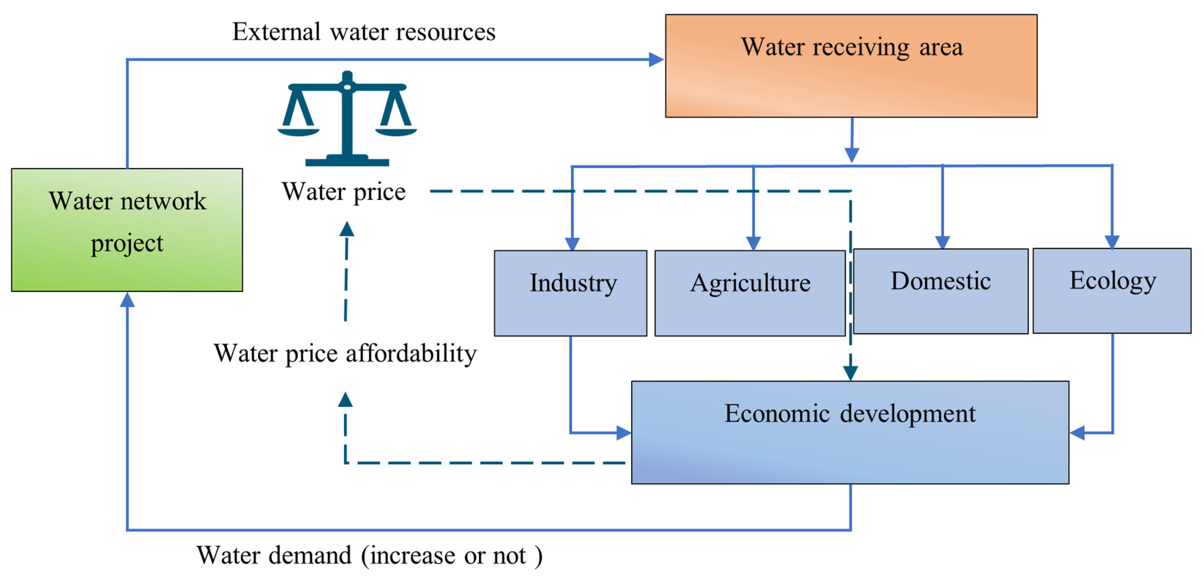
Ignoring extreme weather events such as severe droughts in the water network supply mode, the water receiving area’s strategy for determining the amount of water to be transferred is based on considerations of water demand, water price affordability, and the input–output relationship of water usage, as shown in Figure 1. Water price affordability typically refers to the ability of consumers to pay for water at a given price level. Viewing the water receiving area from a macro perspective, water price affordability analysis [19,20,21] should assess the economic capacity to bear the cost of water usage. While the input level of water resources affects the output of water productivity, input–output relationship analysis can explain how water usage in economic activities leads to value generation [22]. Balancing these two factors ensures that the water transfer scheme is both economically sustainable and beneficial for the development of the water receiving area. It can also promote more refined water demand management. Meanwhile, does an increase in available water resources and the resulting economic growth reverse or regulate the water price affordability? How these two variables influence each other has not yet been thoroughly explored through theoretical and empirical analysis. Better water price affordability provides the conditions for higher water pricing. Higher water prices, as a market signal, could encourage consumers to improve water use efficiency, thus reducing water waste and alleviating the rigid water scarcity issues. In contrast, lower water prices may lead to the overuse of water resources, lower water efficiency, and difficulty in achieving a balanced supply–demand relationship for water resources in the water receiving area. Therefore, the interaction between water price affordability and economic growth warrants further research to provide theoretical support for water resource management and pricing policies.

Many studies have attempted to integrate factors such as resource scarcity [23,24], water accessibility [25], and timely adjustment mechanisms within urban network scales [26] into water pricing models. In addition, studies have explored the interrelationships between water price and water demand, as well as consumption and water use efficiency. These include water demand functions [27,28], input–output models [29], Cobb–Douglas production functions [30], the water price and usage efficiency model [31], water insecurity and its measurement [32], and economic development equations based on the environmental Kuznets curve (EKC) [33]. The EKC hypothesis, first proposed and tested by Grossman and Krueger [34,35], posits that environmental degradation, including pollution emissions and natural resource use, often follows an inverted U shape as economic development progresses [36,37]. The EKC relationship between water use and economic growth has been both proposed and empirically verified [38]. Scholars later identified a nonlinear relationship with a distinct inverted U shape between per capita water usage and income in 65 countries from 1962 to 2008, aligning with the EKC framework and confirming its robustness [39]. Further research has attempted to elucidate the relationship between income growth and freshwater use, providing limited support for the EKC hypothesis, with the results being highly dependent on the choice of datasets and statistical technique [40]. In contrast, some studies argue that there is no evidence for the existence of an EKC relationship between urban water usage and economic growth [41], and that industrial water use does not comply with the inverted U shape [42]. Empirical research on water’s EKC relationship is often sensitive to the choice of control variables, and many studies fail to account for the dynamic interactions between water usage, economic growth, and their feedback effects. Although Hao et al. [33] proposed a simultaneous equations model to explore the bilateral causal relationship between water usage and economic growth, specialized research on the interactive mechanisms between water price affordability within the water network supply mode and the economic growth of a water-receiving area remains limited. This gap constitutes the core research focus of the present study, and it is therefore urgent to undertake further research to address the global water scarcity challenge. Firstly, this study assumes that the water price under the water network supply mode is a comprehensive reflection of the value of water resources, incorporating factors such as water network infrastructure construction costs, scarcity value, and water-saving regulation functions. Considering the background of China’s water network engineering and the associated water supply mode, this study treats the current water pricing strategy in the water receiving area as reflecting the upper bound of water price affordability. Subsequently, this study constructs a simultaneous equations model to examine the relationship between water price and economic growth, drawing on econometric theory. A hypothetical variable for the weighted average water price in the water receiving area is introduced to analyze its impact on economic growth. Furthermore, the relationship between industrial water price and industrial economic growth is empirically analyzed. Finally, based on the analysis of the results, this study discusses the principles of water transfer decision-making and pricing strategies in water receiving areas.

This study makes the following contributions: (1) From the perspective of water prices reflecting the value of water resources, the critical role of water resources in economic and social development in water-scarce regions is highlighted. (2) The comprehensive water price in the water receiving area follows an ‘N’-shaped curve in relation to per-capita GDP growth. When the weighted average water price $\overline{P}\in \left(1.5317,2.4373\right)$, the economic growth is suppressed. (3) The industrial water price in the water receiving area corresponds to the second upward phase of the ‘N’-shaped curve relationship with industrial GDP growth. (4) Overall, economic growth in the water receiving area can enhance water price affordability, and early implementation of industrial water price increases can drive structural transformation, promoting water-saving behavior and efficient water use. This study provides robust empirical evidence for water transfer decision-making and the optimization of the water pricing mechanism in water receiving areas. The relationship between industrial water prices in the water receiving area and industrial per capita GDP growth is currently located in the second ascending segment of the ‘N’-shaped curve.

2. Material and Methods

2.1. Study Area

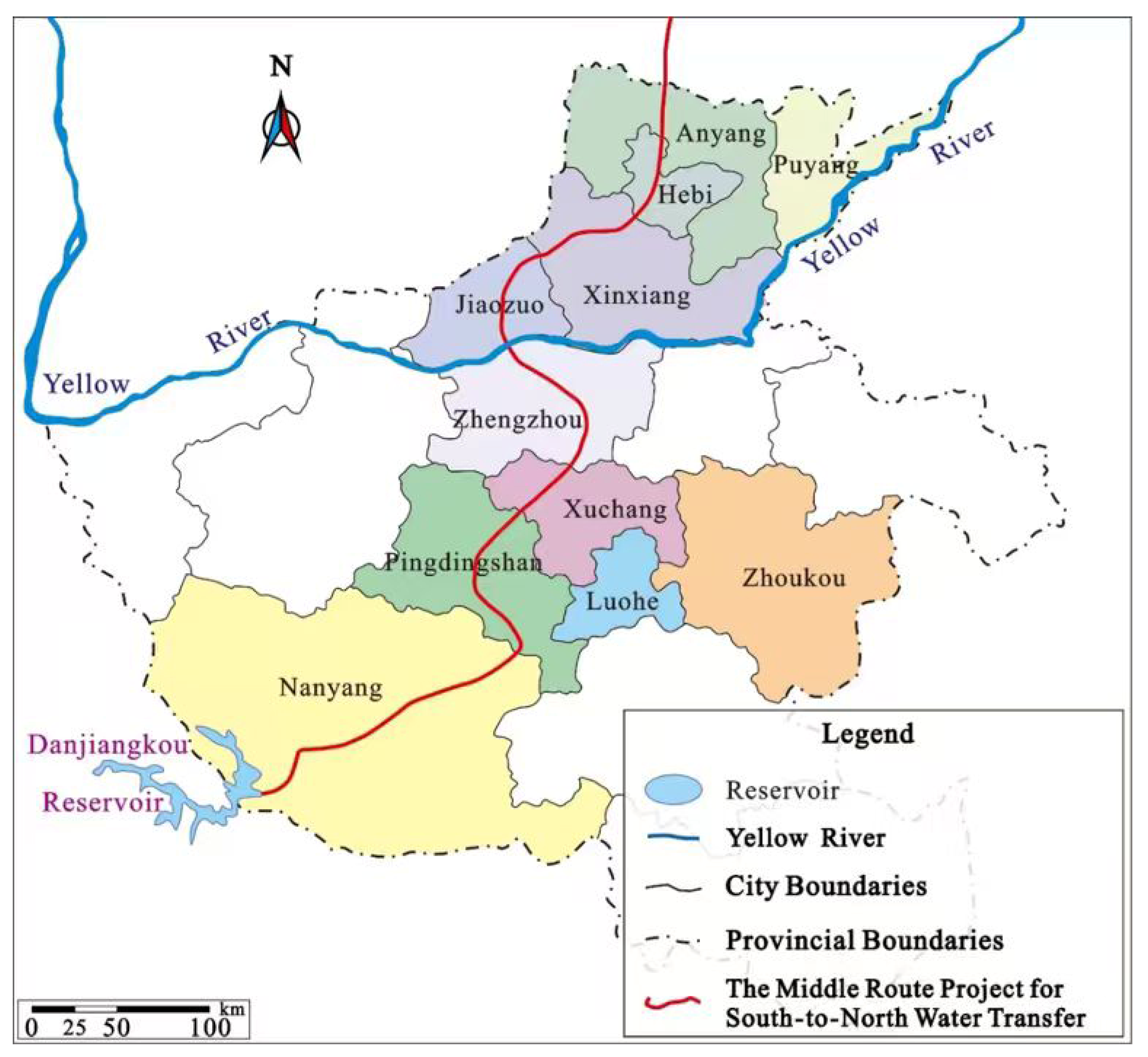
The Middle Route of the South-to-North Water Diversion Project is a prominent water network project initiative in China, with construction beginning in 2002 and operations commencing on 12 December 2014. The project diverts water from the Danjiangkou Reservoir, located across the provinces of Hubei and Henan, and supplies it to 14 large- and medium-sized cities in four provinces and municipalities: Henan, Hebei, Beijing, and Tianjin. This project has significantly improved water resource conditions in northern China, thereby facilitating regional economic and social development. This study focuses on the water receiving area of Henan province, examining the interrelationship between water price and economic growth since the project’s inception. The Henan water receiving area includes 12 provincial cities along the Middle Route of the South-to-North Water Diversion Project: Nanyang, Pingdingshan, Luohe, Zhoukou, Xuchang, Jiaozuo, Zhengzhou, Xinxiang, Hebi, Anyang, Puyang, and Zhumadian. Zhumadian was added as a new water receiving area in 2022. Considering that the full impact of external water resources has not yet been realized, this study limits its scope to the other 11 water receiving cities to provide a more comprehensive and continuous assessment. The spatial distribution of these 11 water receiving cities is characterized by continuity, with homogeneity in economic structure, population characteristics, and technological development, which aligns with the EKC hypothesis [43]. The distribution of these 11 water receiving cities in Henan province is shown in Figure 2.

2.2. Methodology

2.2.1. Simultaneous Equations Model

The water receiving areas comprehensively utilize both external and local water sources, generating water use benefits, including economic, social, and ecological benefits [44,45]. Among these, the level of economic benefits directly impacts the per capita income of society, which in turn influences the water price affordability of water users. In this research, per capita GDP is used to represent regional economic growth. Drawing on the EKC hypothesis, and recognizing that water resources serve as both input and production factors, this study puts forward that there exists a bidirectional influence between water price affordability and economic growth in the water receiving area. To explore this relationship, a simultaneous equations model was developed. Unlike the standard reduced-form EKC model, the cubic GDP coefficient has been verified as significant [43]. Additionally, recent research suggests that the fluctuation characteristics of higher-order polynomials better reflect the evolving water demand patterns in regional development [46]. Therefore, this simultaneous equations model includes the squared and cubed terms of the explanatory variables to capture potential nonlinear relationships between the explanatory variables and the dependent variables, thereby better reflecting the multi-stage-effect relationship between water price and economic growth, enhancing the model’s goodness of fit. In this model, the first equation is the water price equation, in which per capita GDP serves as the explanatory variable and water price is the explained variable. The second equation is the economic growth equation, where water price is the explanatory variable and per capita GDP is the explained variable. These two equations present a bilateral reflection of the relationship between water price and economic growth in the water receiving area. The transmission mechanism of economic growth on water price occurs mainly through three pathways: (1) Economic growth raises residents’ disposable income and enterprises’ profits, which improves water price affordability and creates space for water price adjustment. (2) Economic growth promotes the transformation and upgrading of the industrial structure, changes the structure of water demand, and further affects the level and structure of water prices. (3) Sustained economic growth enhances the local fiscal capacity to support water network construction and operation, thus affecting the cost allocation and final pricing level of water supply. This bi-directional mechanism constitutes the theoretical basis of the simultaneous equations model. At the same time, considering the restrictive effects of factors such as per capita available water, income levels, and consumption patterns on water pricing, variables such as per capita available water, per capita income, urbanization rate, and the consumer price index for urban residents are incorporated as control variables in the water price equation. Additionally, to account for the contributions of total available water resources, foreign trade, and enterprise profits to economic development, control variables such as total water consumption, foreign investment utilization, and profits of large-scale industrial enterprises are included in the economic growth equation. The simultaneous equations model is represented as follows:

$$\left\{\begin{array}{l}{P}_{st}=e_s+{\varphi }_{1}G{I}_{st}+{\varphi }_{2}G{I}_{st}^2+{\varphi }_{3}G{I}_{st}^3+{\varphi }_{4}RW+{\varphi }_{5}S{R}_{st}+{\varphi }_{6}C{Z}_{st}+{\varphi }_{7}X{F}_{st}+r_{st}\\ G{I}_{st}=f_s+d_1{P}_{st}+d_2{P}_{st}^2+d_3{P}_{st}^3+d_4{Q}_{st}+d_{5}W{Z}_{st}+d_{6}IL{R}_{st}+z_{st}\end{array}\right.$$

(1)

In Equation (1), $P_{st}$ represents the unit water price in the water receiving area $s$ in the $t$-th year, measured in CNY/m³. $G{I}_{st}$ represents the economic growth of the water receiving area $s$ in the $t$-th year, expressed as per capita GDP in CNY/person. Regarding the control variables, $R{W}_{st}$ represents the per capita available water in the water receiving area $s$ in the $t$-th year, measured in m³/person; $S{R}_{st}$ represents the per capita disposable income, measured in CNY/person; $C{Z}_{st}$ represents the urbanization rate of the water receiving area, expressed as a percentage (%); $X{F}_{st}$ represents the urban residents’ consumer price index, which is dimensionless; $Q_{st}$ represents the total available water, measured in 100 million m³; $W{Z}_{st}$ represents foreign investment utilization, measured in units of CNY 100 million; $IL{R}_{st}$ represents the profits of industrial enterprises above the designated size, measured in units of CNY 1 million. Meanwhile, $e_s$ and $f_s$ are constants, representing the time-invariant characteristics of the water price and economic development in the water receiving area. ${\varphi }_1,{\varphi }_2,{\varphi }_3,{\varphi }_4,{\varphi }_5,{\varphi }_6,{\varphi }_7$ and $d_1,d_2,d_3,d_4,d_5,d_6$ are the parameters to be estimated in the two equations. $r_{st}$ and $z_{st}$ represent the random error terms in the two equations, respectively. Compared to the panel data random effects model, the fixed effects model takes into account the potential correlations between the explanatory variables and the estimated coefficients, allowing for a more precise analysis of the effects. Furthermore, to mitigate heteroscedasticity, all model variables are transformed into logarithmic form. As a result, Equation (1) is reformulated as follows:

$$\left\{\begin{array}{l}\ln P_{st}=e_s+{\varphi }_1\ln G{I}_{st}+{\varphi }_2{\ln }^{2}G{I}_{st}+{\varphi }_3{\ln }^{3}G{I}_{st}+{\varphi }_4\ln RW+{\varphi }_5\ln S{R}_{st}+{\varphi }_6\ln C{Z}_{st}+{\varphi }_7\ln X{F}_{st}+r_{st}\\ \ln G{I}_{st}=f_s+d_1\ln P_{st}+d_2{\ln }^2{P}_{st}+d_3{\ln }^3{P}_{st}+d_4\ln Q_{st}+d_5\ln W{Z}_{st}+d_6\ln IL{R}_{st}+z_{st}\end{array}\right.$$

(2)

In Equation (2), the water price equation does not account for variables such as Q, WZ, and ILR, which have significant explanatory power for economic growth but do not directly influence water price setting, thus satisfying exogeneity. The economic growth equation does not include variables such as RW, SR, CZ, and XF, which have an indirect driving effect on economic growth but directly influence water price setting and water consumption, thus satisfying the exclusivity constraint criterion. During model application, this specification requires further data validation and adjustment. The number of excluded exogenous variables in each equation is greater than or equal to the number of endogenous variables minus 1. The rank of the coefficient matrix of the excluded exogenous variables is equal to the number of endogenous variables minus 1 (rank = 1). Variables excluded from the economic growth equation affect water demand but do not directly affect economic growth, which meets the exclusion restriction and ensures the exogeneity of instrumental variables. Furthermore, this study conducts the Hausman endogeneity test (${\chi }^2=18.72$, $P=0.000$) and Sargan over-identification test (${\chi }^2=4.16$, $P=0.125$). The model is therefore fully identified, which ensures the rationality and credibility of the empirical results.

2.2.2. Weighted Average Water Price Variable Setting and Its Rationality Analysis

In China, water pricing is linked to the type of water usage, and for the same amount of water, the economic benefits vary significantly across different sectors. Therefore, the relationship between water price and economic growth can be analyzed based on different water use categories, such as industry and agriculture. In this case, water price and benefit indicators are defined for each category, such as industrial water price and industrial GDP. Due to the unavailability of disaggregated data such as industrial water cost at the city-year level, for analyzing the relationship between water price and economic growth comprehensively, a weighted average water price $\overline{P_{st}}$ for the water receiving area needs to be established, i.e., as follows:

$$\overline{P_{st}}={\displaystyle \frac{{\displaystyle \sum Q_{st.i}{P}_{st,i}}}{{\displaystyle \sum Q_{st,i}}}}$$

(3)

In Equation (3), $Q_{st,i}$ represents the water consumption of type $i$ in the water receiving area $s$ during the year $t$, and $P_{st,i}$ represents the unit water price of type $i$ in the water receiving area $s$ during the year $t$. It should be noted that the weighted average water price $\overline{P_{st}}$ is a hypothetical value, used to represent the overall level of water use investment in the water receiving area.

Furthermore, water pricing in Henan’s water receiving areas is determined by price authorities, guided by the core principles of cost compensation and user affordability. Any adjustment to water prices must undergo public consultation and a feasibility assessment of residents’ and enterprises’ capacity to bear the costs. Therefore, the established water price represents the maximum acceptable level under the current economic development stage. This study uses the government-set water price to reflect the upper bound of acceptable price, rather than directly measuring water price affordability. Analysis of the water price information and per capita disposable income for domestic water use in Henan’s water receiving areas from 2013 to 2023 indicates that the increase in domestic water prices is significantly lower than the increase in residents’ income, and the current water prices have not exceeded the payment capacity of water users. Relevant studies [19,20] have pointed out that the government-guided water price in developing countries can be regarded as a reasonable proxy for water price affordability when micro panel data are unavailable, which provides theoretical support for this assumption. To avoid circular reasoning, this study additionally adopts the total water expenditure indicator, which covers residential, industrial, and agricultural water expenditure, as an alternative measure of water price affordability, and conducts corresponding robustness tests. Meanwhile, this study uses per capita available water as an external instrumental variable to address bias caused by endogeneity between water expenditure and income. Compared to similar studies that explore the connection between total water usage and economic growth [33,47], this research illustrates water resource utilization in the water receiving area following the implementation of a water network supply mode, analyzed from the input–output perspective. Furthermore, the empirical research method employed can accurately reflect the effects of water pricing implementation, making it highly reliable.

2.3. Data Basis

The time span of this study extends from 2013 to 2023, encompassing both the construction and operational phases of the Middle Route of the South-to-North Water Diversion Project. The water price adjustments experienced by the water receiving areas after the operation of the project commenced are included. This study required the collection of data from 11 provincial cities, including per capita GDP, industrial water consumption volume, agricultural water consumption volume, residential water consumption volume, total water consumption volume, water price information, per capita disposable income, and other related information. These data were obtained from the annual Water Resources Bulletin, the Statistical Yearbook of Henan Province, and the websites of local Development and Reform Commissions. Water expenditure share was calculated by matching water price, water consumption, and economic data for each city and each year during 2013–2023. Per capita GDP and other socio-economic data are adjusted to 2010 constant prices using Fixed-base Price Index method (consumer price index for overall economic data and per capita disposable income; producer price index for industrial products for industry-related data), with 2010 as the base year (price index = 100). The price indices are derived from the Statistical Yearbook of Henan Province (2014–2024), and linear interpolation was used for supplementing missing price index data. A total of 121 sample points were collected, ensuring the accuracy and reliability of the fixed-effect model estimation. The statistical information for the panel data is shown in

Table 1. Descriptive statistics of relevant variables.

Variables		Symbols	Mean	Std. Dev.	Maximum	Minimum
Per capita GDP		$GI$	51,256.63	19,111.9	113,139	20,359
Water expenditure	Residential water expenditure	HWE	113.36	32.86	210.20	45.94
	Industrial water expenditure	IWE	15.68	6.53	31.34	8.12
	Agricultural water expenditure	AWE	0.47	0.31	1.29	0.20
Per capita disposable income		$SR$	24,320.93	5467.89	43,785	12,906
Water consumption	Agricultural water consumption volume	$Q_1$	7.31	4.31	16.532	1.488
	Industrial water consumption volume	$Q_2$	2.62	1.74	7.943	0.515
	Residential water consumption volume	$Q_3$	2.8	2.11	11.208	0.614
	Total water consumption	$Q$	12.73	5.97	25.25	3.193
Industrial workforce		$R{S}_2$	106.81	55.39	238.28	26.31
Industrial per capita GDP		$G{I}_2$	129,951.6	55,345.85	293,328.6	37,519.26
Agricultural water price		$P_1$	0.14	0.02	0.25	0.105
Industrial water price		$P_2$	4.48	0.86	5.95	2.8
Residential water price		$P_3$	3.21	0.61	4.4	2.05
Weighted average water price		$\overline{P}$	1.75	0.77	3.92	0.78
Per capita available water		RW	250.64	111.72	656.74	96.30
Urbanization rate		CZ	52.92	9.10	80.00	34.80
Urban Consumer Price Index		XF	101.73	0.96	103.30	98.50
Proportion of the secondary industry		IR	48.32	9.06	67.37	28.78
Foreign investment utilization		WZ	56.23	65.25	321.33	0.0014
Profits of industrial enterprises above the designated size		ILR	247.64	220.57	1079.14	2.64

Note: Ecological water consumption has been included in statistics since 2019 and its price information is unavailable, so it was not incorporated into the total water consumption data. Industrial per capita GDP was calculated using the ratio of industrial GDP to the size of the industrial workforce. Some agricultural water price data are missing, and the minimum estimated value of 0.105 was derived through interpolation. White test results show that heteroskedasticity is effectively mitigated after the log transformation, with the statistic decreasing from ${\chi }^2=12.34$ ($P<0.01$) to ${\chi }^2=3.21$ ($P=0.078$). The proportion of interpolated data is less than 5% of the total sample.

.

3. Model Estimation

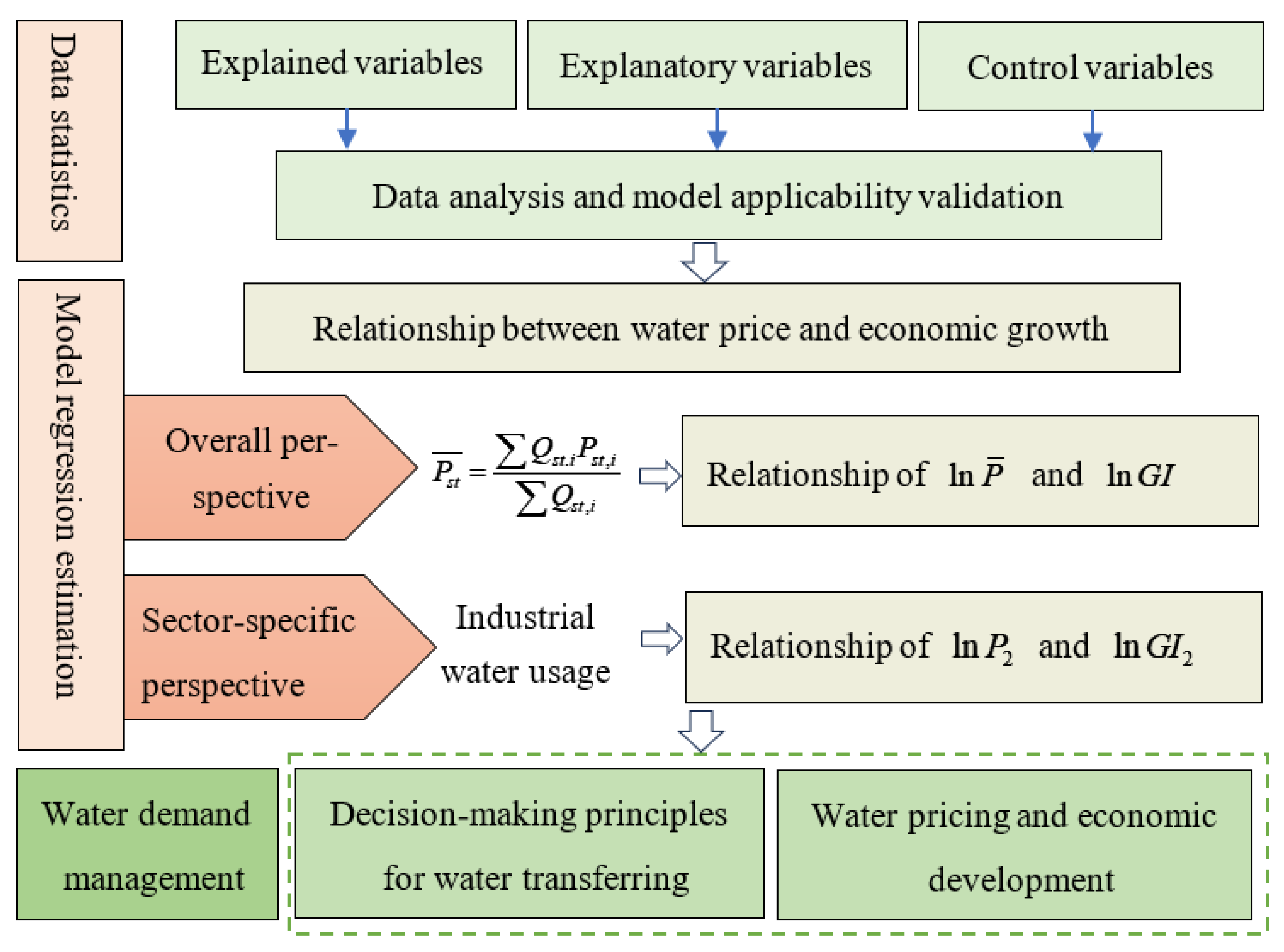
Before conducting regression estimation with the constructed model, a preliminary analysis of the variation patterns of variables such as water price and economic growth was performed based on statistical data, verifying the applicability of the simultaneous equations model. Subsequently, based on Equation (2), two groups of panel data were established from both overall and sector-specific perspectives, and regression estimation was carried out. Using the results from the simultaneous equation model regression estimation, we assessed the intrinsic relationship between water price and economic growth. Finally, based on the analysis of related variables, the decision-making principles for water transfer and pricing were proposed. The framework for this study is shown in Figure 3.

3.1. Data Analysis and Model Applicability Verification

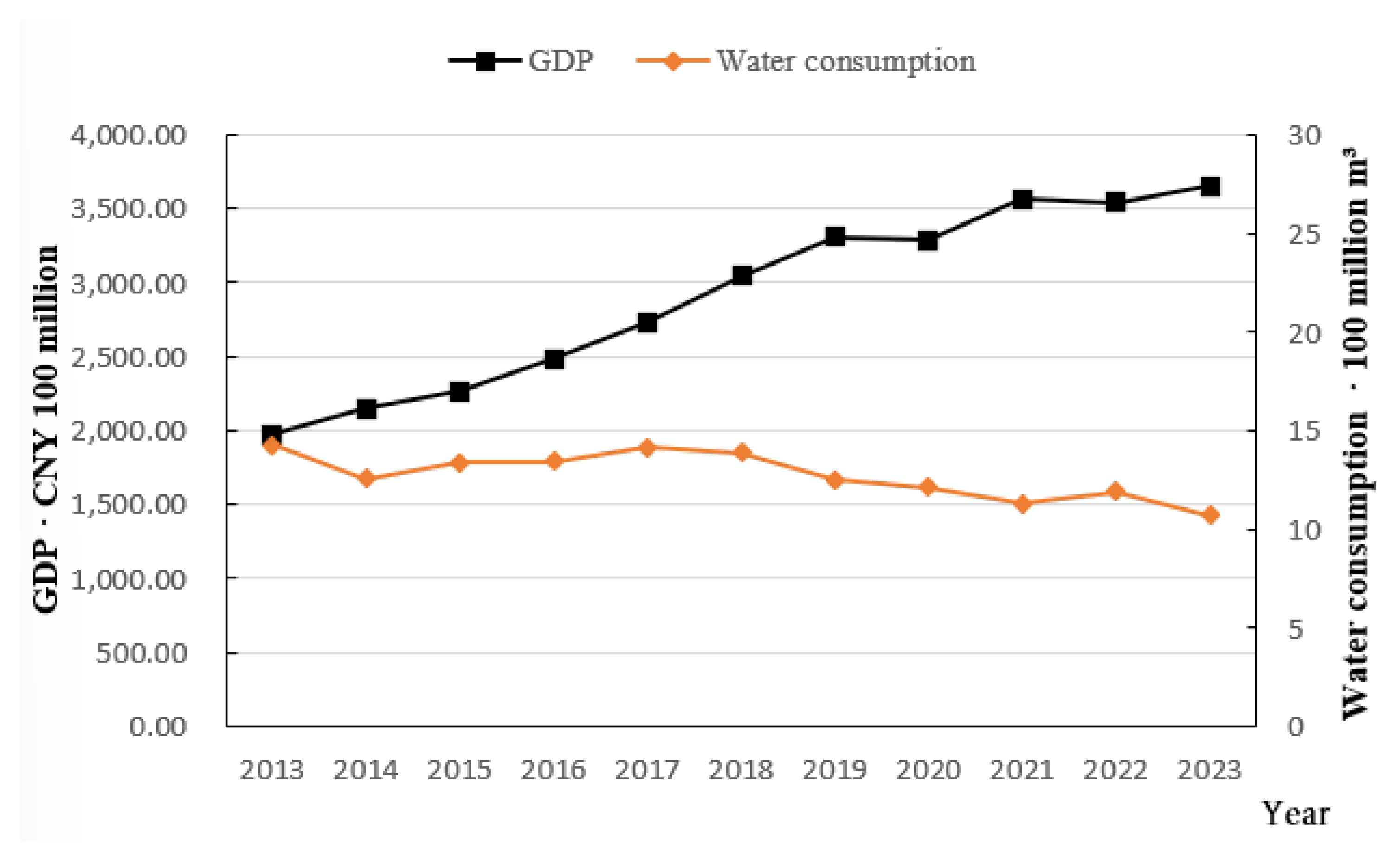
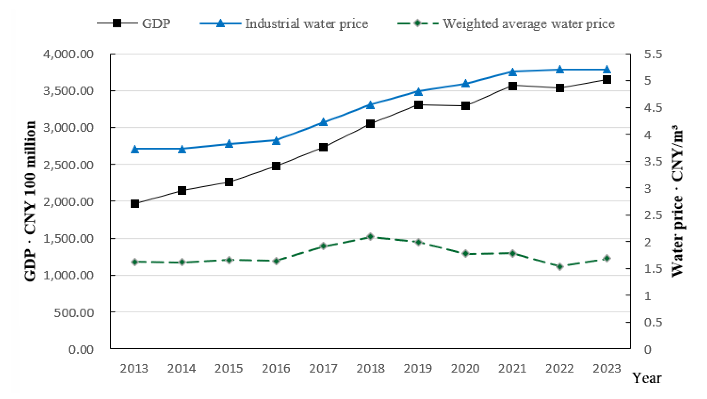
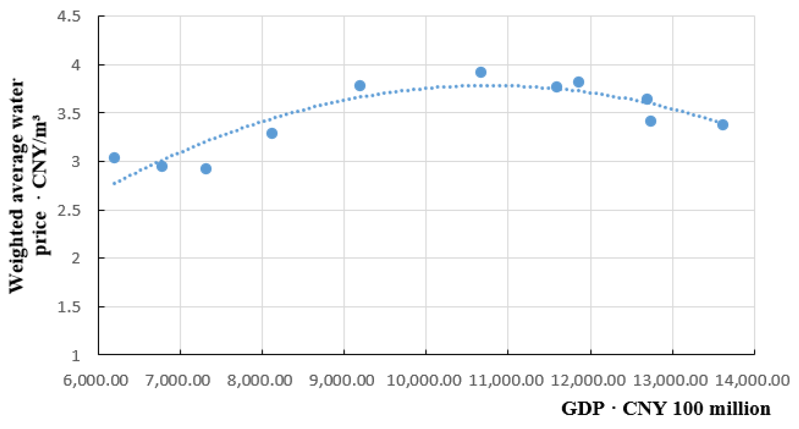
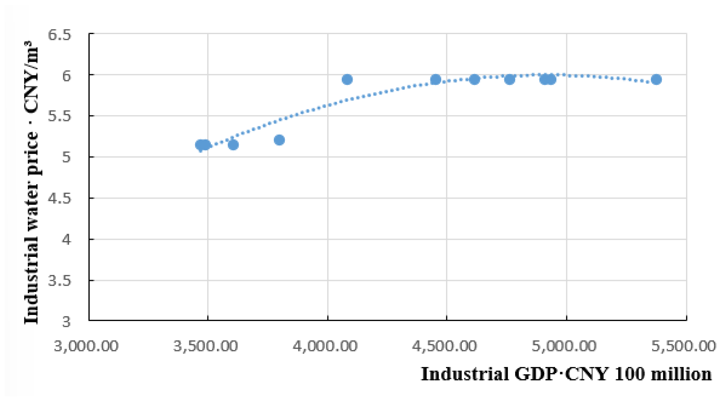
Water price, as an economic tool for adjusting the supply–demand equilibrium, first affects water consumption, and through this medium, influences the economic development of the water receiving area. This study began by analyzing the trends in the average GDP and total water consumption of the water receiving area from 2013 to 2023, based on the collected panel data, as shown in Figure 4. The trends in average GDP, industrial water price, and the weighted average water price (calculated using Equation (3)) are depicted in Figure 5. From 2013 to 2023, the GDP of the Henan water receiving area exhibited continuous growth, with a slight decline in 2020. In contrast, total water consumption in the water receiving area showed a consistent downward trend. As illustrated in Figure 5, the increase in industrial water prices in the water receiving area was closely aligned with GDP growth. The weighted average water price initially increased but then decreased, contradicting the overall trend of rising water prices across various industries. This discrepancy can primarily be attributed to the consistent reduction in water consumption across industries. The data reveal that rising water prices have not hindered economic growth; instead, they have exerted a positive impact on both the overall economic development of the water receiving areas and the efficient utilization of water resources. Taking Zhengzhou as a case study, a scatter plot illustrating the relationship between the weighted average water price and GDP is presented in Figure 6, while the relationship between the industrial water price and industrial GDP is analyzed and shown in Figure 7. The blue dashed curve represents the fitted trend line of the relationship between the weighted average water price and GDP in Zhengzhou, which exhibits an inverted ‘U’ shape, providing preliminary evidence for a Kuznets curve relationship between water price and economic growth. Additionally, Zhengzhou’s industrial GDP continued to grow alongside rising industrial water prices, indicating that higher industrial water price did not suppress economic growth. However, over time, the growth rate of industrial GDP gradually slowed and eventually began to decline. Since 2017, Zhengzhou’s industrial water price has stabilized, making it difficult to predict future trends. The most likely shape of the fitting curve appears to be an ‘N’ shape, further supporting the existence of Kuznets curve relationship between water prices and economic growth.

3.2. Model Regression Estimation

As analyzed in Section 3.1, under the influence of water price adjustments, water consumption in the water receiving area shows a downward trend, while economic development continues to grow. It is essential to directly examine the interaction between water prices and economic growth. Moreover, data from the study area indicate that the secondary industry, primarily dominated by manufacturing, contributes an average of 48.32% to the average GDP, making it a significant contributor to economic growth in the water receiving area. Based on the construction of a simultaneous equations model for the water receiving area, two groups of empirical analyses are carried out:

(1) First group: Analyzing the relationship between the weighted average water price and per capita GDP in the water receiving area, without distinguishing between different types of water usage.

(2) Second group: Analyzing the relationship between industrial water price and industrial per capita GDP in the water receiving area, with differentiation of water usage types.

These two empirical analyses explore the relationship between water price and economic growth from both an overall and sector-specific perspective.

3.2.1. Variable Non-Stationarity Test

Considering that time series data often exhibit complex changes, it is essential to conduct non-stationarity tests before modeling and performing regression analysis on panel data to assess whether the data are stationary. If the data are found to be non-stationary, differencing must be applied to transform them into stationary series. This study employs two widely used unit root test methods: the LLC test (Levin–Lin–Chu test) and the ADF test (Augmented Dickey–Fuller test). The results of the panel data unit root tests are presented in

Table 2. Unit root test.

Variables	LLC Test			ADF Test
	Statistic Value	p-Value	Results	Statistic Value	p-Value	Results
$\ln \overline{P}$	−3.32599 ***	0.0004	stationary	12.4452	0.9475	non-stationary
$\ln P_2$	−8.18556 ***	0	stationary	25.5006	0.2737	non-stationary
$\ln GI$	1.28822	0.9012	non-stationary	6.55337	0.9994	non-stationary
$\ln G{I}_2$	−2.6856 ***	0.0036	stationary	27.0343	0.2099	non-stationary
$\ln Q$	−4.27301 ***	0	stationary	28.981	0.1454	non-stationary
$\ln Q_2$	−4.57596 ***	0	stationary	21.375	0.4977	non-stationary
$\ln RW$	−2.90134 ***	0.0019	stationary	18.5501	0.6729	non-stationary
$\ln SR$	−79.1935 ***	0	stationary	196.16 ***	0	stationary
$\ln CZ$	0.06123	0.5244	non-stationary	5.17152	0.9999	non-stationary
$\ln XF$	0.23977	0.5947	non-stationary	11.4321	0.968	non-stationary
$\ln WZ$	2.0302	0.9788	non-stationary	2.77958	1	non-stationary
$\ln ILR$	0.04096	0.5163	non-stationary	18.9837	0.6463	non-stationary

Note: *** indicates parameters that are statistically significant at the level of 1%.

. Except for per capita disposable income, all other variables are deemed non-stationary. Due to inconsistencies between the LLC and ADF test results, first-order differencing was applied to each cross-sectional series in the panel data. Unit root tests were then performed on the differenced series, as shown in

Table 3. First-differenced unit root test.

Variables	LLC Test			ADF Test
	Statistic Value	p-Value	Results	Statistic Value	p-Value	Results
$\ln \overline{P}$	−8.91562 ***	0	stationary	44.3751 ***	0.0032	stationary
$\ln P_2$	−4.55975 ***	0	stationary	33.2733 ***	0.0581	stationary
$\ln GI$	−4.94656 ***	0	stationary	30.5639 ***	0.094	stationary
$\ln G{I}_2$	−9.05908 ***	0	stationary	48.6723 ***	0.0009	stationary
$\ln Q$	−10.4315 ***	0	stationary	66.5024 ***	0	stationary
$\ln Q_2$	−6.20374 ***	0	stationary	36.9581 ***	0.0239	stationary
$\ln RW$	−8.01767 ***	0	stationary	43.4467 ***	0.0042	stationary
$\ln SR$	−11.8742 ***	0	stationary	59.7747 ***	0	stationary
$\ln CZ$	−5.89586 ***	0	stationary	36.2272 ***	0.0287	stationary
$\ln XF$	−7.40274 ***	0	stationary	29.308 ***	0.0933	stationary
$\ln WZ$	−4.54008 ***	0	stationary	32.7806 ***	0.065	stationary
$\ln ILR$	−12.3726 ***	0	stationary	56.7668 ***	0.0001	stationary

Note: *** indicates parameters that are statistically significant at the level of 1%.

. According to the majority rule and economic significance criterion, a variable is classified as integrated of order one if both its LLC and ADF test statistics are significant at the 1% level after first-order differencing. Additionally, variables such as water price and GDP are identified as trending variables, and their first-order integration aligns with the general characteristics of economic time series. The results clearly demonstrate that all variables become stationary after the first differencing, confirming that they are integrated of order one. This satisfies the prerequisite for the panel cointegration analysis.

3.2.2. Cointegration Relationship Test

When the original panel data are non-stationary, directly conducting regression analysis may lead to spurious results. Therefore, based on the first-order integration discussed earlier, it is necessary to further determine whether a long-term stable relationship exists between the series, which is assessed through a cointegration test. Cointegration analysis helps avoid the problem of spurious regression in non-stationary panel data. If the cointegration test confirms the presence of such a relationship, subsequent regression analysis can more accurately capture the long-term interactions between variables, yielding results that are both economically meaningful and statistically robust. To support the following model regression analysis, cointegration tests were conducted on two sets of panel data, tailored to the requirements of the two empirical studies:

(1) First group panel data: weighted average water price ($\ln \overline{P}$), per capita GDP ($\ln GI$), per capita disposable income ($\ln SR$), per capita available water ($\ln RW$), urbanization rate ($\ln CZ$), urban consumer price index ($\ln XF$).

(2) Second group panel data: industrial water price ($\ln P_2$), industrial per capita GDP ($\ln G{I}_2$), per capita disposable income ($\ln SR$), per capita available water ($\ln RW$), urbanization rate ($\ln CZ$), urban consumer price index ($\ln XF$), foreign investment utilization ($\ln WZ$), profits of large-scale industrial enterprises ($\ln ILR$).

In this study, the Pedroni test and Kao test were employed, with the results presented in

Table 4. Cointegration test results of the first group panel data.

Methods	Statistics	Value	p-Value	Weighted Statistic Value	p-Value
Pedroni test	Panel v-Statistic	−1.371817	0.9149	−3.195289	0.9993
	Panel rho-Statistic	3.649303	0.9999	3.714719	0.9999
	Panel PP-Statistic	−10.55175	0	−13.25101	0
	Panel ADF-Statistic	−5.958122	0	−6.208634	0
	Group rho-Statistic	5.140578	1
	Group PP-Statistic	−13.87041	0
	Group ADF-Statistic	−5.601637	0
Kao test	ADF	−4.152867	0

and

Table 5. Cointegration test results of the second group panel data.

Methods	Statistics	Value	p-Value	Weighted Statistic Value	p-Value
Pedroni test	Panel v-Statistic	−1.677934	0.9533	−3.287947	0.9995
	Panel rho-Statistic	3.820949	0.9999	4.02231	1
	Panel PP-Statistic	−8.327505	0	−9.997823	0
	Panel ADF-Statistic	−4.763307	0	−4.378797	0
	Group rho-Statistic	5.129491	1
	Group PP-Statistic	−12.58498	0
	Group ADF-Statistic	−4.855844	0
Kao test	ADF	−4.272011	0

. Based on the outcomes of these tests, a long-term stable cointegration relationship can be seen between the two sets of panel data. This suggests that these variables share an equilibrium relationship in the long run, allowing for further empirical analysis through model regression estimation.

3.2.3. Panel Error Correction Model Estimation

Given that the panel data series are confirmed to be cointegrated at the 1% significance level (Table 4 and Table 5), a stable long-term equilibrium relationship exists between water price and economic growth. To further investigate the short-term dynamic adjustment mechanism from deviations in the long-term equilibrium-to-re-equilibrium process, a panel error correction model (ECM) was constructed for the two groups of panel data in this study. This model effectively captures the interactive relationship between the short-term fluctuations and long-term equilibrium of variables. The Generalized Weighted Least Squares (GWLS) method was employed for estimating the panel ECM, addressing issues of heteroscedasticity, contemporaneous correlation, and autocorrelation. The estimation results of the core parameters are reported in

Table 6. ECM estimation results of the two groups.

Variables	$\mathbf{\Delta }\mathbf{ln}\overline{\mathit{P}}$ (GWLS)	$\mathbf{\Delta }\mathbf{ln}\mathit{G}\mathit{I}$ (GWLS)	Variables	$\mathbf{ln}\mathit{G}\mathit{I}$ (GWLS)	$\mathbf{ln}\mathit{G}\mathit{I}$ (3SLS)
Constant	−0.0342(0.021)	0.0893 *** (0.020)	Constant	−0.0281 (0.019)	0.0765 *** (0.018)
$\Delta \ln {\overline{P}}_{t-1}$	0.1872 ** (0.074)	−0.0921 * (0.053)	$\Delta \ln P_{2,t-1}$	0.2105 ** (0.069)	−0.0843 * (0.049)
$\Delta \ln GI$	0.2145 *** (0.061)	-	$\Delta \ln G{I}_2$	0.1987 *** (0.058)	-
$\Delta \ln G{I}_{t-1}$	-	0.3254 *** (0.059)	$\Delta \ln {GI}_{2,t-1}$	-	0.2968 *** (0.055)
$\Delta \ln SR$	0.3876 *** (0.050)	0.2241 *** (0.041)	$\Delta \ln SR$	0.3542 *** (0.048)	0.2015 *** (0.038)
$\Delta \ln RW$	0.0421 * (0.022)	0.0158 (0.018)	$\Delta \ln RW$	0.0394 * (0.021)	0.0122 (0.017)
$\Delta \ln CZ$	0.2013 ** (0.082)	0.1532 ** (0.065)	$\Delta \ln CZ$	0.1892 ** (0.078)	0.1411 ** (0.061)
$\Delta \ln XF$	0.4251 *** (0.055)	0.0876 * (0.047)	$\Delta \ln XF$	0.3981 *** (0.052)	0.0798 * (0.043)
$EC{M}_{t-1}$	−0.1562 *** (0.038)	−0.2814 *** (0.052)	$EC{M}_{t-1}$	−0.1723 *** (0.035)	−0.3025 *** (0.048)
N	110	110	N	110	110
Adjusted $R^2$	0.582	0.643	Adjusted $R^2$	0.615	0.689

Note: ***, **, and * indicate parameters that are statistically significant at the level of 1%, 5%, and 10%, respectively.

. It is evident that the coefficients of the error correction terms for both data series are negative and statistically significant at the 1% level, verifying the existence of a negative feedback adjustment effect when variables deviate from long-term equilibrium. Notably, the absolute values of the error correction coefficients are relatively small, revealing that the self-correction speed of the system is slow. This indicates that the adjustment from short-term deviation to long-term equilibrium presents obvious time lag, and the policy effect of water price adjustment cannot be realized rapidly. Moreover, this finding strengthens the robustness of the long-term equilibrium relationship proposed by the simultaneous equation model in this study, offering strong support for short-term adjustment dynamics.

3.2.4. Simultaneous Equations Model Regression Estimation

Based on the complete time series analysis, including the unit root test (Table 2 and Table 3), cointegration test (Table 4 and Table 5), and ECM estimation (Table 6), the simultaneous equations model is further regressed by GWLS and 3SLS methods, which ensures the rationality and completeness of the model estimation. In the study area, there are regional differences in water usage behavior, consumption habits, and levels of socio-economic development among residents. As a result, the panel data may be affected by issues such as heteroscedasticity and autocorrelation. Before selecting the appropriate regression estimation method, tests for heteroscedasticity between groups, contemporaneous correlation between groups, and autocorrelation within groups were conducted, as shown in

Table 7. Results of tests for between-group heteroscedasticity, inter-group temporal correlation, and intra-group autocorrelation.

Contents	The First Group Panel Data		The Second Group Panel Data
	Statistic Value	p-Value	Statistic Value	p-Value
Between-group heteroscedasticity (Modified Wald test)	56.27	0	78.08	0
Inter-group temporal correlation (Pesaran’s test)	−2.207	0.0273	−2.159	0.0308
Intra-group autocorrelation (Wooldridge test)	36.709	0.0001	36.709	0.0001

. The test results indicate that both panel data groups exhibit problems related to heteroscedasticity, contemporaneous correlation, and autocorrelation within their data structures. For the subsequent analysis, the Generalized Weighted Least Squares (GWLS) method was employed for model regression to ensure the reliability of the estimation results. The simultaneous equations model, as formulated in Equation (2) in Section 2.2, is presented alongside the GWLS estimation results in

Table 8. Estimation results from GWLS and 3SLS methods of the simultaneous equations model (for the first group).

Weighted Average Water Price Equation			Economic Growth Equation
Explanatory Variables	$\mathbf{\Delta }\mathbf{ln}\overline{\mathit{P}}$ (GWLS)	$\mathbf{\Delta }\mathbf{ln}\overline{\mathit{P}}$ (3SLS)	Explanatory Variables	$\mathbf{ln}\mathit{G}\mathit{I}$ (GWLS)	$\mathbf{ln}\mathit{G}\mathit{I}$ (3SLS)
$\ln GI$	699.5319 *** (3.43)	606.2342 *** (3.26)	$\ln \overline{P}$	6.1371 *** (3.14)	5.8923 *** (2.75)
${\ln }^{2}GI$	−64.6477 *** (−3.51)	−56.4357 *** (−3.07)	${\ln }^2\overline{P}$	−10.6416 *** (−3.11)	−9.2615 *** (−3.02)
${\ln }^{3}GI$	1.9911 *** (3.39)	1.2364 *** (2.12)	${\ln }^3\overline{P}$	5.3858 *** (3.05)	5.9876 *** (2.99)
$\ln SR$	−0.0854 (−0.32)	−0.0604 (−0.31)	$\ln Q$	−0.2089 ** (−2.13)	−0.1946 ** (−2.02)
$\ln RW$	−0.4597 *** (−5.07)	−0.4007 *** (−5.92)	$\ln WZ$	−0.0525 (−1.49)	−0.0375 (−1.53)
$\ln CZ$	0.4029 (1.04)	0.3391 (0.89)	$\ln ILR$	0.0428 (0.67)	0.0505 (0.57)
$\ln XF$	6.6211 ** (2.12)	6.4532 ** (2.01)
_cons	−2.55 × 103 *** (−3.57)	−2.46 × 103 *** (−3.45)	_cons	9.8136 *** (7.69)	1.2345 ** (3.15)
N	121	121		121	121
Adjusted $R^2$	0.3528	0.3615		0.4092	0.4123

Note: Values in parentheses are cluster-robust standard errors at the city level. ** p < 0.0506, *** p < 0.0106. Omitting the estimation results of the exogenous variables introduced in the 3SLS estimation.

and

Table 9. Estimation results from GWLS and 3SLS methods of the simultaneous equations model (for the second group).

Industrial Water Price Equation			Industrial Economic Growth Equation
Explanatory Variables	$\mathbf{ln}{\mathit{P}}_2$ (GWLS)	$\mathbf{ln}{\mathit{P}}_2$ (3SLS)	Explanatory Variables	$\mathbf{ln}\mathit{G}{\mathit{I}}_2$ (GWLS)	$\mathbf{ln}\mathit{G}{\mathit{I}}_2$ (3SLS)
$\ln G{I}_2$	−3.1427 * (−1.52)	−3.127 * (−1.28)	$\ln P_2$	105.5664 ** (1.80)	101.8792 ** (1.75)
${\ln }^{2}G{I}_2$	0.4183 ** (1.88)	0.5018 ** (1.95)	${\ln }^2{P}_2$	−74.0049 * (−1.74)	−77.2291 * (−1.85)
${\ln }^{3}G{I}_2$	−0.0156 ** (−1.98)	−0.0253 ** (−1.78)	${\ln }^3{P}_2$	17.3402 * (1.87)	17.0012 * (1.84)
$\ln SR$	0.3525 *** (3.40)	0.4021 *** (3.61)	$\ln Q_2$	−0.3510 *** (−6.26)	−0.2633 *** (−4.74)
$\ln RW$	−0.1634 *** (−3.80)	−0.1137 *** (−3.46)	$\ln WZ$	0.0143 (0.75)	0.0256 (0.86)
$\ln CZ$	−0.0167 (−0.11)	−0.0208 (−0.13)	$\ln ILR$	0.0357 (1.05)	0.0309 (1.17)
$\ln XF$	0.7352 (0.47)	0.6827 (0.52)
_cons	0.0000 (.)	0.0000 (.)	_cons	−38.6250 (−1.45)	−36.7413 (−0.70)
N	121	121		121	121
Adjusted $R^2$	0.3528	0.3607		0.4092	0.4177

Note: Values in parentheses are cluster-robust standard errors at the city level. * p < 0.106, ** p < 0.0506, *** p < 0.0106. Omitting the estimation results of the exogenous variables introduced in the 3SLS estimation.

. Given that both water price and per capita GDP are economic variables, Three-Stage Least Squares (3SLS) was further utilized to eliminate simultaneous equation bias and evaluate the robustness of the estimation results. The results from the 3SLS method, as shown in Table 8 and Table 9, are consistent with those from the GWLS regression, confirming the robustness of the estimates. According to statistics, the COVID-19 pandemic had certain impacts on industrial production in water receiving areas in 2022, while industrial water efficiency kept improving and local industrial water prices remained largely unchanged. The estimated coefficients and their significance are highly consistent, whether 2022 is included or excluded. The results in Table 6, Table 8 and Table 9 show that the long-term elasticity reflects the steady-state relationship between water price and economic growth in the long run, while the error correction term captures the short-term adjustment toward this equilibrium. To test the sensitivity of data interpolation, the model regression was also re-estimated by excluding observations with interpolated agricultural water prices. The results show that the signs, magnitudes, and significance of core coefficients remain highly consistent, confirming that the interpolation does not affect the reliability of the model.

To further verify the rationality of the functional relationship setup between explanatory and explained variables in the simultaneous equations model, this study compared the goodness-of-fit between the quadratic simultaneous equations model (without the cubic term) and the cubic model (with the quadratic and cubic terms) using the Akaike Information Criterion (AIC) and Bayesian Information Criterion (BIC); the comparison for the first group is shown in

Table 10. Goodness-of-fit comparison between quadratic and cubic models (for the first group).

Model	AIC	BIC	Log Likelihood
Quadratic model (without the cubic term)	142.67	168.91	−62.34
Cubic model	128.34	156.72	−53.17

. It is indicated that the inclusion of the cubic term substantially improves the model fit. This confirms that the ‘N’-shaped nonlinear relationship is not a spurious result of random fluctuations, but a statistically significant characteristic of the study data.

3.2.5. Robustness Test Using Water Expenditure Indicator

To verify the reliability of the regression estimation results, this study replaced the weighted average water price with water expenditure share and re-estimated the simultaneous equations model, as shown in

Table 11. Robustness tests using total water expenditure indicator.

Water Expenditure Equation			Economic Growth Equation
Variables	$\mathbf{ln}\mathit{W}\mathit{E}$ (GWLS)	$\mathbf{ln}\mathit{W}\mathit{E}$ (3SLS)	Variables	$\mathbf{ln}\mathit{G}\mathit{I}$ (GWLS)	$\mathbf{ln}\mathit{G}\mathit{I}$ (3SLS)
$\ln GI$	102.4312 *** (3.88)	99.1252 *** (3.65)	$\ln WE$	6.1024 *** (3.21)	5.8962 *** (2.94)
${\ln }^{2}GI$	−71.3482 *** (−2.12)	−68.5641 *** (−1.83)	${\ln }^{2}WE$	−10.1223 *** (−3.09)	−9.3123 *** (−3.01)
${\ln }^{3}GI$	16.7856 *** (1.61)	16.0324 *** (1.51)	${\ln }^{3}WE$	5.1201 *** (3.14)	4.8954 *** (3.10)
_cons	−36.1245 (−1.52)	−34.7812 (−1.47)	_cons	3.836 *** (2.91)	2.8245 ** (1.36)
Adjusted $R^2$	0.4002	0.4189	Adjusted $R^2$	0.347	0.405

Note: *** and ** indicate statistical significance at the 1% and 5% levels, respectively.

. The results show that the coefficients of the total water expenditure and its square and cube terms remain statistically significant at the 1% and 5% levels. The signs of the core coefficients are completely consistent with the baseline regression results. The relationship between total water expenditure and economic growth still presents a significant ‘N’-shaped curve. These results confirm that the substitution of the water expenditure share indicator does not change the core conclusions of this study, indicating that the relationship between overall water price and economic growth in the Henan water receiving area is robust and reliable.

4. Results and Analysis

4.1. Relationship Analysis of $\ln \overline{P}$ and $\ln GI$

4.1.1. Expression of the Simultaneous Equations Model

Table 8 shows that the coefficients of per capita GDP and its square and cube terms in the weighted average water price equation, where water use types are not differentiated, are all are statistically significant. Similarly, the coefficients of the weighted average water price and its square and cube terms in the economic growth equation are also statistically significant. These two equations can be expressed in the following simultaneous form:

$$\left\{\begin{array}{cc}\hfill \ln \overline{P}& =-2550+699.5319\ln GI-64.6477{\ln }^{2}GI+1.9911{\ln }^{3}GI-0.0854\ln SR\hfill \\ & -0.4597\ln RW+0.4029\ln CZ+6.62\ln XF+r\hfill \\ \hfill \ln GI& =9.8136+6.1371\ln \overline{P}-10.6416{\ln }^2\overline{P}+5.3858{\ln }^3\overline{P}-0.2089\ln Q\hfill \\ & -0.0525\ln WZ+0.0428\ln ILR+z\hfill \end{array}\right.$$

(4)

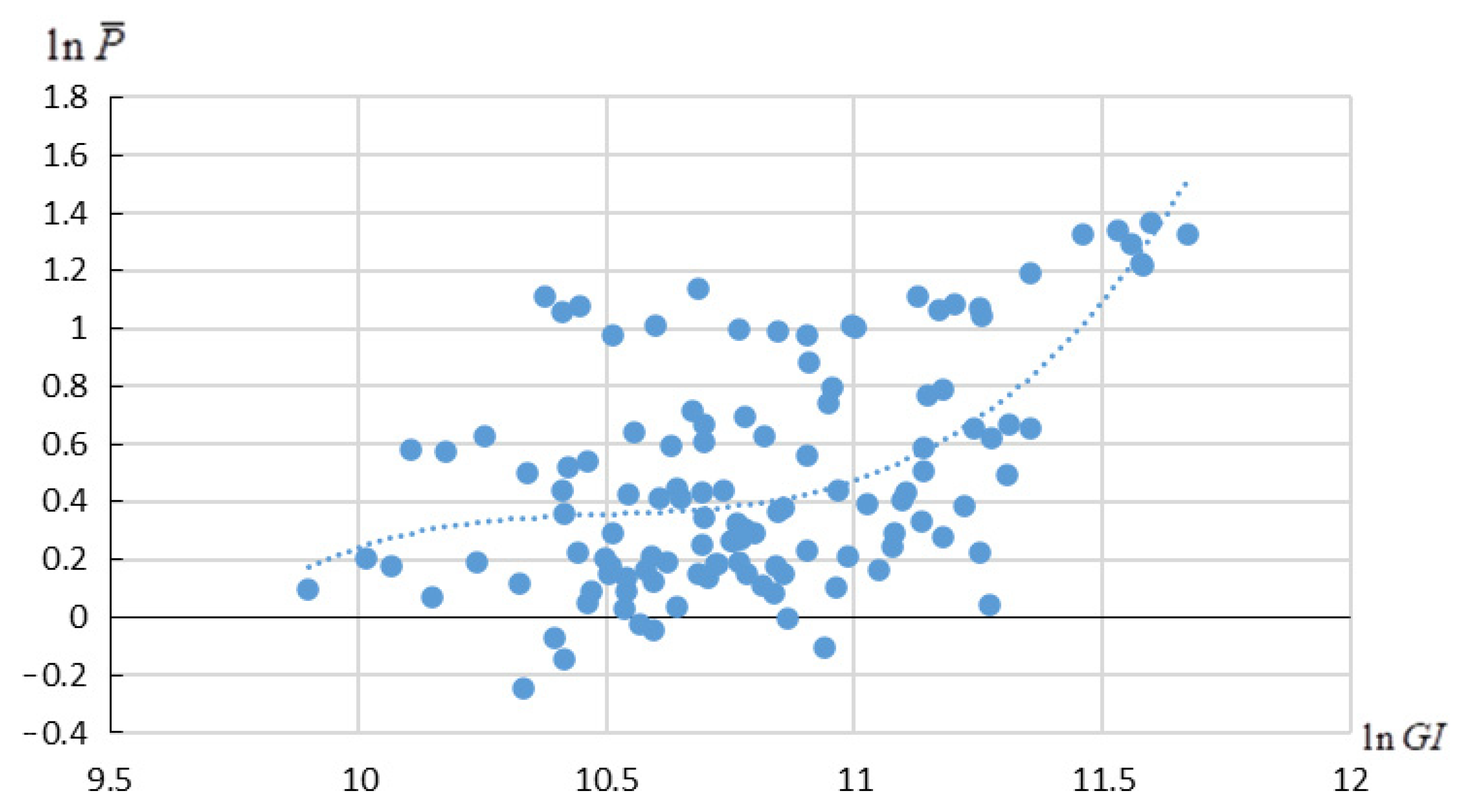
In Equation (4), r and z represent the random error terms. To further illustrate the relationship visually, a coordinate system was constructed with $\ln GI$ as the horizontal axis and $\ln \overline{P}$ as the vertical axis. A scatterplot was generated using the data series from the study area during the research period, and a curve was fitted according to Equation (4) to demonstrate the relationship. It was found that the relationship between $\ln \overline{P}$ and $\ln GI$ follows an ‘N’-shaped curve, as shown in Figure 8. This result confirms the presence of a stable long-run equilibrium relationship between overall water price and economic growth.

4.1.2. Results Analysis

Based on the regression estimation results of the simultaneous equations model, the first-order derivatives were calculated and can be displayed as follows:

$${\ln }^{\prime }\overline{P}=699.5319-2\times 64.6477\ln GI+3\times 1.9911{\ln }^{2}GI$$

(5)

$${\ln }^{\prime }GI=6.1371-2\times 10.6416\ln \overline{P}+3\times 5.3858{\ln }^2\overline{P}$$

(6)

Setting the first-order derivatives to zero reveals the existence of turning points in the functions of the simultaneous equations. The turning point for economic growth is derived from the weighted average water price equation, producing values of $\ln GI=10.6720$ and $\ln GI=10.9736$ Meanwhile, the turning points for the weighted average water price are $\ln \overline{P}=0.4264$ and $\ln \overline{P}=0.8909$. The ‘N’-shaped curve relationship between the weighted average water price and economic growth shows that when $\overline{P}\in \left(1.5317,2.4373\right)$ (Delta 95% CI, $\overline{P}\in \left(1.5149,2.4662\right)$), economic growth in the research area is slightly suppressed. Within this range of economic growth, once the water price exceeds the affordable threshold, it will surpass users’ capacity to pay and have a negative impact on economic growth, further supporting the rationale for using the current water price to reflect the upper bound of affordability.

Panel data analysis reveals differentiated water price status across the study area. Zhengzhou has moved beyond the stage where rising water prices constrain economic growth. In comparison, Pingdingshan, Hebi, Xuchang, and Luohe remain trapped in the growth-inhibiting interval at the prevailing water price level. The remaining cities, including Anyang, Xinxiang, Jiaozuo, Puyang, Nanyang, and Zhoukou, register water prices below the regional average. After eliminating the interference of water consumption structure in weighted average water price calculation, the results show that moderate price rises within reasonable affordability will not curb economic growth but instead promote long-term economic development in Zhengzhou, Pingdingshan, Xuchang, and Luohe.

4.2. Relationship Analysis of $\ln P_2$ and $\ln G{I}_2$

4.2.1. Expression of the Simultaneous Equations Model

Similarly, as shown in Table 9, the coefficients of industrial per capita GDP, as well as its square and cube terms in the industrial water price equation, where water usage types are differentiated, demonstrate statistical significance in the water receiving areas. Likewise, the coefficients of industrial water price, along with its square and cube terms in the industrial economic growth equation, also exhibit statistical significance in the water receiving areas. The industrial water price equation and the industrial economic growth equation can be expressed in the following forms:

$$\left\{\begin{array}{cc}\hfill \ln P_2& =-3.1427\ln G{I}_2+0.4183{\ln }^{2}G{I}_2-0.0156{\ln }^{3}G{I}_2+0.3525\ln SR\hfill \\ & -0.1634\ln RW-0.0167\ln CZ+0.7352\ln XF+r_2\hfill \\ \hfill \ln G{I}_2& =-38.625+105.5664\ln P_2-74.0049{\ln }^2{P}_2+17.3402{\ln }^3{P}_2\hfill \\ & -0.351\ln Q_2+0.0143\ln WZ+0.0357\ln ILR+z_2\hfill \end{array}\right.$$

(7)

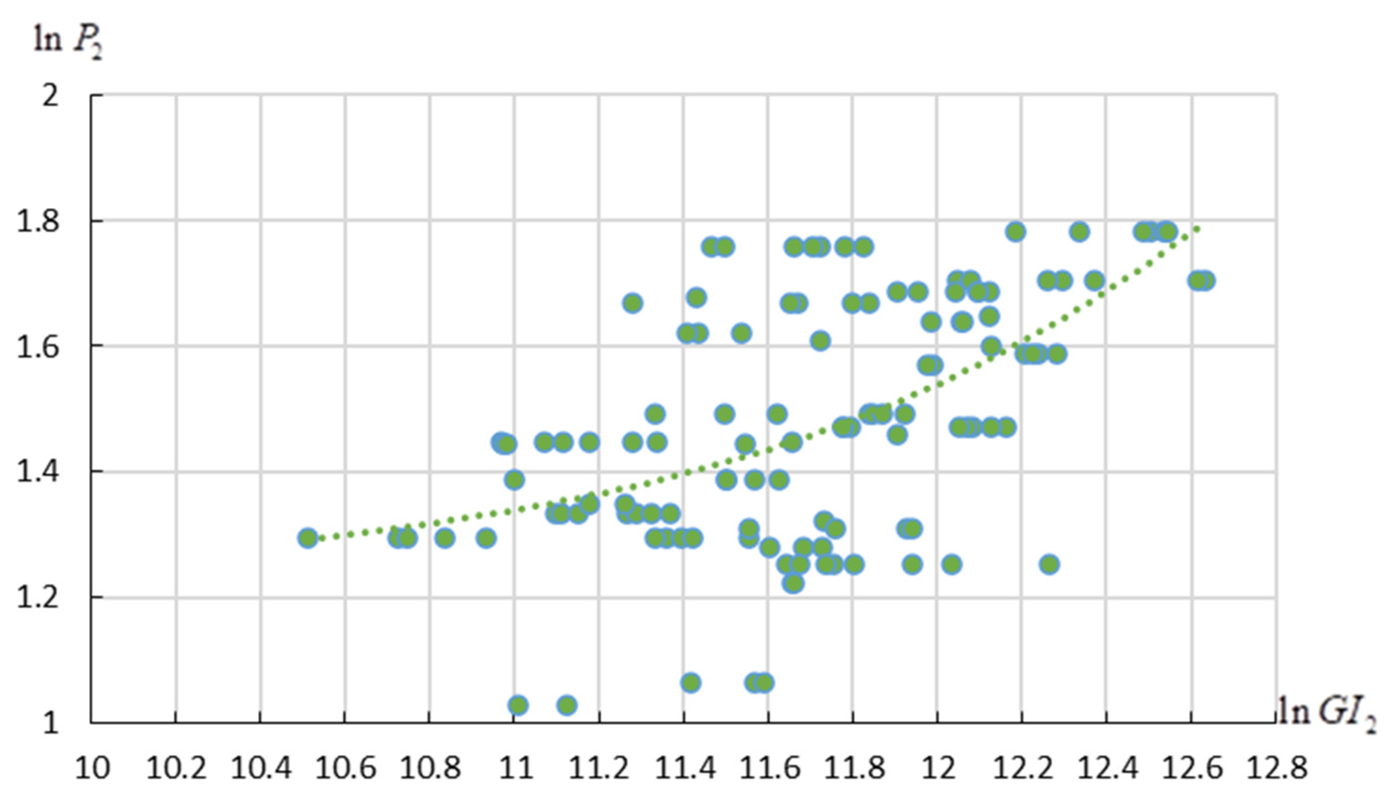
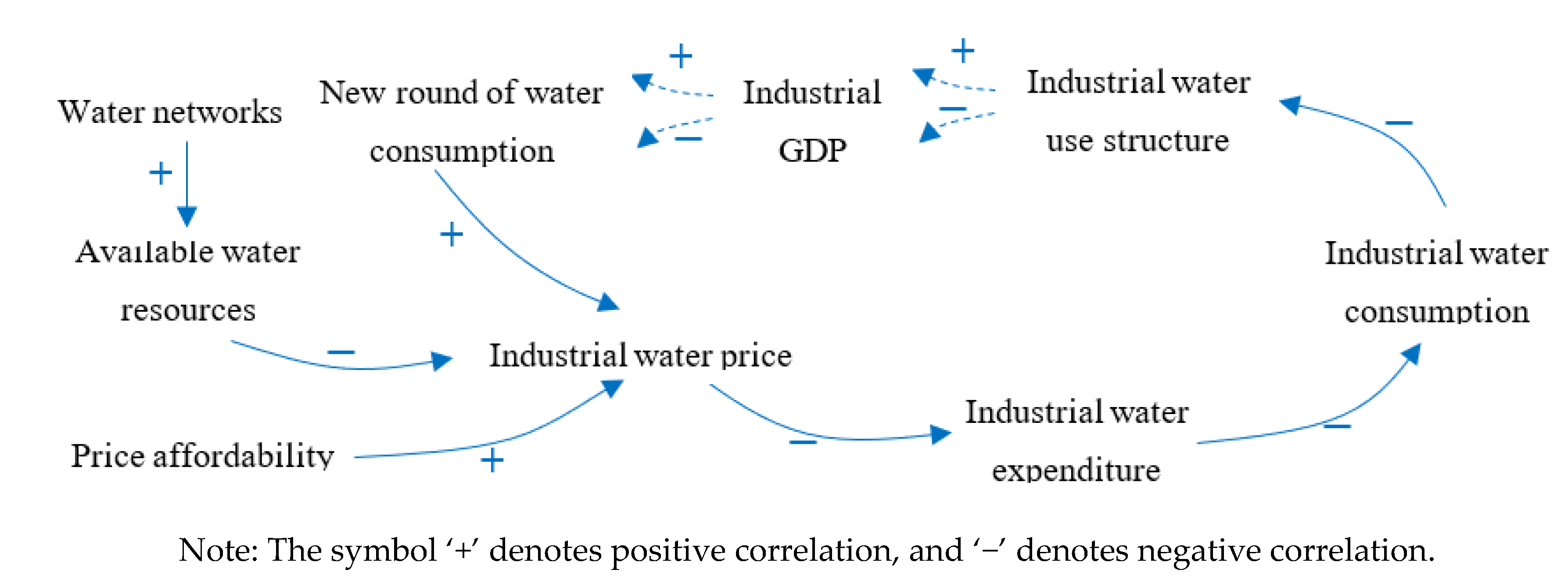
In Equation (7), $r_2$ and $z_2$ represent the random error terms. To further illustrate the relationship, a coordinate system was constructed with $\ln G{I}_2$ as the horizontal axis and $\ln P_2$ as the vertical axis. A scatterplot was generated using the data series from the study area, and a curve was fitted according to Equation (7). The analysis indicates that the relationship corresponds to the second upward phase of the ‘N’-shaped curve, as shown in Figure 9. This result also implies that a stable long-run equilibrium relationship exists between industrial water price and industrial growth. The interaction mechanism between industrial water price and industrial growth is shown in Figure 10.

4.2.2. Results Analysis

Based on the regression estimation results of the simultaneous equations model, the first-order derivatives of the system were calculated and as follows:

$${\ln }^{\prime }{P}_2=-3.1427+2\times 0.4183\ln G{I}_2-3\times 0.0156{\ln }^{2}G{I}_2$$

(8)

$${\ln }^{\prime }G{I}_2=105.5664-2\times 74.0049\ln P_2+3\times 17.3402{\ln }^{2}P$$

(9)

By setting the first derivative to zero and transforming it into a quadratic equation, it was found that these two equations has no real roots. The curve generated by the system of equations does not exhibit any inflection points, indicating a positive correlation between industrial water price and industrial economic growth. Consequently, water resources are crucial for industrial production, and industrial enterprises bear the responsibility for their rational utilization and protection. It is important to note that due to limited data during the study period in the research area, as well as the fact that industrial water prices have not yet exceeded the water price affordability of the water receiving area, this conclusion does not fully capture their comprehensive interaction. With the continuous growth of industrial production and the rising demand for industrial water, the finite nature of water resources will inevitably intensify the water supply–demand conflict. Therefore, adjusting industrial water prices to enable optimal allocation of water resources will become an inevitable trend in the foreseeable future. In the first group of empirical findings, a positive correlation was observed between economic growth improvements and the increased price affordability of the water receiving area. The ongoing development of water network infrastructure provides favorable conditions for this trend.

4.3. Influence Analysis of Control Variables

4.3.1. Overall Economic Growth of the Water Receiving Area

The estimated results of the simultaneous equations model, without distinguishing between water use types, provide the following analysis of the influence of control variables on the water price–economic growth relationship: (1) Per capita available water and consumer price index: Both per capita available water and the urban residents’ consumer price index significantly influence water price. Specifically, per capita available water is negatively correlated with water price, and this relationship is statistically significant at the 1% level. This suggests that an abundance of water resources limits the potential for increases in water price. Furthermore, the region’s relatively weak awareness of water conservation may contribute to slower improvements in water use efficiency [48,49]. (2) Total water consumption and economic growth: Total water consumption significantly impacts economic growth, while other control variables do not show significant effects. This suggests that sufficient water resources are foundational to industrial development, agricultural production, and economic growth. Research indicates that the South-to-North Water Diversion Project has raised the economic growth level of water receiving counties by 6.1% and alleviated water resource constraints in these areas [50]. Moreover, the development and operation of water network projects, along with the interconnectivity of water resources, have promoted spatial clustering between regions, further fostering industrial growth and economic development.

4.3.2. Industrial Economic Growth of the Water Receiving Area

When differentiating by types of water usage, the estimation results from the simultaneous equations model show the following influence of control variables on the relationship of industrial water price and industrial economic growth in water receiving areas: (1) Per capita available water and per capita disposable income: Both per capita available water and per capita disposable income significantly affect industrial water prices. Specifically, per capita available water is negatively correlated with industrial water price, with statistical significance at the 1% level, while per capita disposable income is positively correlated with industrial water price, significant at the 5% level. In addition to the negative impact of available water resources, the relatively low income levels of urban residents also suppress water price increases. Thus, the continuous improvement in urban residents’ income levels enhances the region’s industrial water price affordability. (2) Industrial water consumption and economic growth. The industrial water consumption volume has a statistically significant impact on industrial economic growth [51,52], while factors such as foreign trade, corporate profits, and others do not show significant effects. This conclusion further underscores the vital role of water resources in driving industrial economic growth. In conclusion, the increase in available water resources supports sustained economic growth, which in turn enhances urban residents’ income levels and consumption patterns, thereby increasing the water price affordability of water receiving areas.

5. Conclusions and Policy Implications

5.1. Conclusions

The development of water network projects in China has facilitated the optimization of water resource allocation, but it has also increased the burden of higher water costs and water prices on water receiving areas. Under the water network supply mode, the water receiving areas make water transfer decisions by balancing regional water scarcity, users’ water price affordability, and the benefits of water usage. This study constructs a simultaneous equations model based on the water EKC hypothesis, assuming that water price affordability is equal to the current water price, to estimate the relationship and interaction between water price and economic growth under the water network supply mode. In this model, water price and per capita GDP, representing economic growth, are treated as explanatory and explained variables, respectively. The model incorporates control variables in each equation to address endogeneity issues in estimation and improve its realism. Using the GWLS estimation method, this study then applied panel data from 11 cities in Henan province, which serve as the water receiving area of the Middle Route of the South-to-North Water Diversion Project, spanning from 2013 to 2023. The analysis considers both general (without distinguishing water usage types) and specific (industrial water usage) perspectives, providing a comprehensive understanding of the relationship between water price and economic growth. The study further assessed the robustness of the estimation using the 3SLS estimation method. The main conclusions are as follows:

(1) In the overall economic growth equation, the coefficients of the linear, quadratic, and cubic terms of the weighted average water price are 6.1371, −10.6416, and 5.3858, respectively, all statistically significant at the 1% level. Similarly, in the industrial economic growth equation, the coefficients of the linear, quadratic, and cubic terms of industrial water price are 105.5664, −74.0049, and 17.3402, respectively, all significant at the 5% level.

(2) The economic growth driven by water resource utilization in water receiving areas exhibits a further feedback relationship with the value of water resources. The comprehensive water price in the water receiving area exhibits an ‘N’-shaped curve in relation to economic growth. In the study area, when the weighted average water price $\overline{P}\in \left(1.5317,2.4373\right)$(Delta 95% CI, $\overline{P}\in \left(1.5149,2.4662\right)$), economic growth is suppressed. This indicates that water price and economic growth generally have a positive correlation, except within a specific water price range. Contrary to the Kuznets curve hypothesis, this study demonstrates that water pricing, when aligned with regional economic development, is crucial, and in this context, increasing water prices alongside economic growth does not hinder economic development.

The industrial water price in the water receiving area corresponds to the second upward phase of the ‘N’-shaped curve relationship with industrial per capita GDP growth. Analysis of the sample data from the study area indicates that raising industrial water prices effectively promotes efficient industrial water consumption, with significance at the 1% level. Analysis of the sample data from the study area indicates that raising industrial water prices effectively promotes efficient industrial water consumption, with significance at the 1% level. Given that the industrial water price in the study area has not yet exceeded the water price affordability threshold, this conclusion indicates that water resources remain crucial for industrial production, even with rising water prices. As industrial production continues to grow and the demand for industrial water increases, adjusting industrial water price becomes crucial for optimal allocation and maximizing water resource efficiency.

(3) Regarding the control variables, per capita available water exerts a statistically significant negative impact on the comprehensive water price in water receiving areas at the 1% level, while the urban consumer price index has a significant positive effect at the 5% level, driving increases in the comprehensive water price. Total water consumption significantly inhibits economic growth in water receiving areas at the 5% level, indicating that water endowment, water use efficiency, and consumption habits jointly influence the formation of water prices and the pathway of economic growth. Industrial water usage shows a significant negative relationship with industrial economic growth at the 1% level, indicating that expanding the scale of industrial water use has not improved water use efficiency. These findings highlight that water prices do not obstruct economic growth, but they are rather an important mechanism to optimize water resource allocation and stimulate economic development within a reasonable range. Industrial production sectors demonstrate stronger resilience to price changes and exert a transmission effect. This study provides robust empirical evidence for the phased and sector-specific formulation of water pricing policies.

5.2. Implications

Water pricing can be effective in steering resource use and non-use in the right direction [53], and the efficient use of local water resources is fundamental to determining the appropriate volume of water to be transferred. Under the water network supply mode, this study explored the relationship between water prices, water consumption, and economic growth and can provide the following decision-making implications for formulating scientific water transfer decisions and water pricing policies in water receiving cities.

(1) Zhengzhou: The current level of the overall water price in Zhengzhou is in a stage beyond the inhibitory zone of economic growth in the ‘N’-shaped curve. In recent years, while the economy has continued to grow, the total water consumption has stabilized at approximately 2.1 billion m³. Considering the local scarcity of water resources and the fact that over 40% of the water supply relies on external sources, it is recommended that water prices be moderately increased. Such progressive price adjustment can steadily foster water-saving awareness and facilitate the long-term improvement of regional water use efficiency.

(2) Pingdingshan, Hebi, Xuchang, and Luohe: These cities are currently experiencing economic growth suppression. In recent years, total water consumption in all four cities declined significantly following the previous round of water price increases and has since stabilized, while the economy and per capita disposable income has grown slowly. Given that water consumption is currently stable, the scale of water transfer can remain unchanged to avoid negatively impacting economic development. Considering that the current water price level is also in the suppressive stage of the ‘N’-shaped curve, a cautious, modest increase in water prices is recommended. Within the acceptable water price range, such an adjustment will not only avoid further suppression but may also promote economic growth. After the careful adjustment of water prices, monitoring the relationship between total water use and economic growth can inform the next round of water transfer strategies. Easing water resource constraints in this gradual way can further stimulate new momentum for long-term economic growth.

(3) Anyang, Xinxiang, Jiaozuo, Puyang, Nanyang, and Zhoukou: These cities currently have water prices lower than the average level, which correlates with a slowdown in economic growth. It is recommended that water transfer strategies in these areas focus primarily on alleviating water resource constraints while promoting both economic and social development. For water allocation, priority water supply should be provided to water users whose economic growth is significantly constrained by water resource availability. Meanwhile, during the initial stage of external water source utilization, local governments may implement policies such as fiscal subsidies and tax incentives to enhance water price affordability. Consequently, water pricing can be gradually adjusted upwards to enhance the effectiveness of water network investments and alleviate fiscal burdens.

Water price policies and water transfer decisions in water receiving areas are interrelated. Factors such as changes in water use patterns, water use efficiency, and the availability of local water resources will all have an impact on their implication. This aligns with research on China’s water rights trading policy [54]. Additionally, ecological protection and the competing interests among multiple water receiving areas must be coordinated through water pricing during the water supply and usage process. Therefore, water receiving areas should develop long-term, multi-dimensional strategies to gradually achieve the desired water allocation and reasonable water price levels. In this process, it is crucial to incorporate predictions of incremental water usage over a defined future period.

6. Limitations and Directions for Further Research

Although this study explores the relationship between water price and economic growth under China’s water network supply mode, there are limitations that must be acknowledged. Firstly, due to limitations in data availability for the study area, capturing the complex variation patterns of research variables across both time and space is challenging. It is suggested that, by alleviating data heterogeneity and weak instrument bias, and further improving estimation accuracy, future research should expand the study area to cover all large and medium cities along the Middle Route of the South-to-North Water Diversion Project. Different water network projects could be selected to conduct a comparative analysis of the relationship between water price and economic growth in different regions, providing a theoretical basis for regional uniform pricing. According to the characteristics of different study regions, the control variables specified in the simultaneous equations model in this study should be appropriately calibrated and adjusted on the basis of empirical statistical analysis. Additionally, from a regional and social development perspective, the non-economic benefits of water resources should be incorporated into comprehensive benefit accounting. Meanwhile, future research should actively conduct theoretical investigations on ecological water pricing, as well as exploring how water price instruments in water-receiving areas can be employed to achieve the coupled and coordinated development of water resources, ecology, and the economy. The methods for measuring the comprehensive impacts of water network supply on regional economic, social, and ecological environments are critical in light of increasing global water scarcity in the future for water transfer decision-making and pricing in water receiving areas.

References

1. Sesma-Martín, D.; Puente-Ajovín, M. The Environmental Kuznets Curve at the thermoelectricity-water nexus: Empirical evidence from Spain. Water Resour. Econ. 2022, 39, 100202. [Google Scholar] [CrossRef]
2. Chopra, R.; Magazzino, C.; Shah, M.L. The role of renewable energy and natural resources for sustainable agriculture in ASEAN countries: Do carbon emissions and deforestation affect agriculture productivity? Resour. Policy 2022, 76, 102578. [Google Scholar] [CrossRef]
3. Vörösmarty, C.J.; Hoekstra, A.Y.; Bunn, S.E.; Conway, D.; Gupta, J. What scale for water governance? Science 2015, 349, 478. [Google Scholar] [CrossRef]
4. Chang, H.Y.; Zhao, Y.; Sang, X.F.; Li, H.H.; He, F.; Zhai, J.Q. Rearch on the coordinated regulation of water resources-food-energy-ecology in Beijing-Tianjin-Hebei Region I: Methods and Model. J. Hydraul. Eng. 2022, 53, 655–665. [Google Scholar] [CrossRef]
5. Cui, C.; Dong, Z.; Han, Y.; Ren, L.; Wang, X.; Si, S. Modelling & assessment of the impact of water network construction on mitigating regional rater supply–demand conflicts: Strategies Approaches for Water Resources Planning and Management. Water Resour. Manag. 2025, 39, 4735–4761. [Google Scholar] [CrossRef]
6. Gao, J.; Zheng, L.; Li, S.; Nie, X.; Huang, K. Analysis of water supply and usage cooperation strategies and evolutionary game among multiple stakeholders in water network. J. Hydrol. Reg. Stud. 2025, 58, 102258. [Google Scholar] [CrossRef]
7. Wu, H.; Li, X.; Lu, H.; Tong, L.; Kang, S. Crop acreage planning for economy- resource- efficiency coordination: Grey information entropy based uncertain model. Agric. Water Manag. 2023, 289, 108557. [Google Scholar] [CrossRef]
8. Zhao, Q.; Tian, G.; Zhu, M.; Li, J.; Wu, X. The Impact of water marketization mechanisms on improving water use efficiency: An empirical study from water rights trading in China. J. Hydrol. Reg. Stud. 2024, 55, 101957. [Google Scholar] [CrossRef]
9. Mohammad-Azari, S.; Bozorg-Haddad, O.; Biswas, A. Water Pricing; Elsevier: Amsterdam, The Netherlands, 2021; pp. 47–61. [Google Scholar] [CrossRef]
10. Bathla, S. Water Resource Potential in Northern India: Constraints and analyses of price and non-price solutions. Environ. Dev. Sustain. 1999, 1, 105–121. [Google Scholar] [CrossRef]
11. Imani, S.; Niksokhan, M.H.; Shali, R. S Fair water re-allocation: Lessons learnt from the perception of Iranian policy-makers about distributive justice. J. Hydrol. 2025, 652, 132675. [Google Scholar] [CrossRef]
12. Li, X.H.; Chen, M.W.; Yan, H. Differences in water use efficiency levels and identification of causes in four major river basins along China’s South-to-North Water Diversion Route. J. Fudan Univ. (Nat. Sci.) 2025, 64, 80–95. [Google Scholar] [CrossRef]
13. Liu, W.X.; Liu, Y.; Wang, Y. Changes in water resources and water consumption in the receiving Area (Beijing-Tianjin-Hebei Region) of the Middle Line of South-to-North Water Diversion Project in the past 20 years. J. Hohai Univ. (Nat. Sci.) 2025, 53, 18–25+153. Available online: https://link.cnki.net/urlid/32.1117.tv.20250205.1615.042 (accessed on 28 May 2026).
14. Momeni, M.; Zakeri, Z.; Esfandiari, M.; Behzadian, K.; Zahedi, S.; Razavi, V. Comparative analysis of agricultural water pricing between Azarbaijan Provinces in Iran and the state of California in the US: A hydro-economic approach. Agric. Water Manag. 2019, 223, 105724. [Google Scholar] [CrossRef]
15. Momeni, M.; Razavi, V.; Zahedi, S.; Momeni, F.; Behzadian, K.; Dolatabadi, N. A study of the required sustainability-driven institutional and behavioural mechanisms to tackle the anticipated implications of agricultural water price shocks: A system dynamics approach. Sci. Rep. 2023, 13, 15397. [Google Scholar] [CrossRef]
16. Maldonado-Devis, M.; Almenar-Llongo, V. A quantile regression approach to the heterogeneity in price elasticity of domestic water demand. Water Resour. Manag. 2024, 38, 4851–4866. [Google Scholar] [CrossRef]
17. Molinos-Senante, M.; Donoso, G. Water scarcity and affordability in urban water pricing: A case study of Chile. Util. Policy 2016, 43, 107–116. [Google Scholar] [CrossRef]
18. Marlim, M.S.; Kang, D. Improving operational efficiency in water distribution network with hourly water pricing to benefit consumers and providers. J. Water Process Eng. 2025, 72, 107457. [Google Scholar] [CrossRef]
19. Martins, R.; Quintal, C.; Teotónio, C.; Antunes, M. Water affordability across and within European countries: A microdata analysis. Util. Policy 2023, 83, 101609. [Google Scholar] [CrossRef]
20. Onda, K.S.; Tewari, M. Water systems in California: Ownership, geography, and affordability. Util. Policy 2021, 72, 101279. [Google Scholar] [CrossRef]
21. Sathre, R. Chapter 16—Affordable and clean energy and water (SDG 7). In Water Matters; Mukherjee, A., Ed.; Elsevier: Amsterdam, The Netherlands, 2024; pp. 191–201. [Google Scholar] [CrossRef]
22. Long, Y.; Liu, Y.; Zhao, T.; Zhang, Z.; Lei, X.; Yang, Y. Optimal allocation of water resources in the middle route of south-to-north water diversion project based on multi-regional input-output model. J. Hydrol. 2024, 637, 131381. [Google Scholar] [CrossRef]
23. Ruijs, A.; Zimmermann, A.; Van Den Berg, M. Demand and distributional effects of water pricing policies. Ecol. Econ. 2008, 66, 506–516. [Google Scholar] [CrossRef]
24. Sahin, O.; Bertone, E.; Beal, C.; Stewart, R.A. Evaluating a novel tiered scarcity adjusted water budget and pricing structure using a holistic systems modelling approach. J. Environ. Manag. 2018, 215, 79–90. [Google Scholar] [CrossRef] [PubMed]
25. Yu, G.; Chen, X.; Tu, Z.; Yu, Q.; Liu, Y.; Yu, H. Modeling water accessibility of natural river networks using the Fine-Grained physical watershed characteristics at the grid scale. Water Resour. Manag. 2017, 31, 2271–2284. [Google Scholar] [CrossRef]
26. Xu, L.; Tu, Z.; Yang, J.; Zhang, C.; Chen, X.; Gu, Y.; Yu, G. A water pricing model for urban areas based on water accessibility. J. Environ. Manag. 2023, 327, 116880. [Google Scholar] [CrossRef] [PubMed]
27. Zhang, S.; Wang, Y. Research on water price and quantity to meet the basic living needs of urban residents based on water conservation. Water Resour. Manag. 2024, 38, 2171–2187. [Google Scholar] [CrossRef]
28. Sun, T.H.; Wang, J.X. Water-saving effects of agricultural water pricing policies: A meta-analysis of the price elasticity of irrigation wa-ter deman. China Popul. Resour. Environ. 2024, 34, 120–132. [Google Scholar] [CrossRef]
29. Xie, R.; Sun, Y.L.; Qiao, H.S. The economic utility and environmental utility analysis of water sources in Hunan province based on input-output model. Chin. J. Manag. Sci. 2013, 21, 677–683. [Google Scholar] [CrossRef]
30. Lü, S.B.; Zhang, L.; Wang, W.C.; Yu, Y.M. Analysis of water consumption and marginal benefit of Henan province. J. Irrig. Drain. 2015, 34, 28–32. [Google Scholar] [CrossRef]
31. Javid, M. Modeling the impact of price and usage efficiency on domestic water demand in Saudi Arabia. Util. Policy 2025, 96, 101971. [Google Scholar] [CrossRef]
32. Charilaou, M.; Hussein, H. Measuring household water insecurity in intermittent supply systems: A context-sensitive index from urban Jordan. Urban Water J. 2026, 1–25. [Google Scholar] [CrossRef]
33. Hao, Y.; Hu, X.L.; Chen, H.Y. On the relationship between water use and economic growth in China: New evidence from simultaneous equation model analysis. J. Clean. Prod. 2019, 235, 953–965. [Google Scholar] [CrossRef]
34. Grossman, G.M.; Krueger, A.B. Environmental impacts of a North American Free Trade Agreement. CEPR Discuss. Pap. 1992, 8, 223–250. [Google Scholar] [CrossRef]
35. Grossman, G.M.; Krueger, A.B. Economic growth and the environment. Nber Work. Pap. 1995, 110, 353–377. [Google Scholar] [CrossRef]
36. Li, J. Kuznets curve, E., balanced growth, and influencing factors: Evidence from economic development in China. Int. J. Clim. Change Strateg. Manag. 2024, 16, 318–336. [Google Scholar] [CrossRef]
37. Sun, S.; Fang, C. Water use trend analysis: A non-parametric method for the environmental Kuznets curve detection. J. Clean. Prod. 2018, 172, 497–507. [Google Scholar] [CrossRef]
38. Cole, M.A. Economic growth and water use. Appl. Econ. Lett. 2004, 11, 1–4. [Google Scholar] [CrossRef]
39. Duarte, R.; Pinilla, V.; Serrano, A. Is there an environmental Kuznets curve for water use? A panel smooth transition regression approach. Econ. Model. 2013, 31, 518–527. [Google Scholar] [CrossRef]
40. Katz, D. Water use and economic growth: Reconsidering the Environmental Kuznets Curve relationship. J. Clean. Prod. 2015, 88, 205–213. [Google Scholar] [CrossRef]
41. Exposito, A.; Pablo-Romero, M.; Sanchez-Braza, A. Testing EKC for urban water Use: Empirical evidence at river basin scale from the Guadalquivir River, Spain. J. Water Resour. Plan. Manag. 2019, 145, 04019005. [Google Scholar] [CrossRef]
42. Lu, W.C. Industrial water use; income; trade, and employment: Environmental Kuznets curve evidence from 17 Taiwanese manufacturing industries. Environ. Sci. Pollut. Res. 2018, 25, 26903–26915. [Google Scholar] [CrossRef]
43. Dinda, S. Environmental Kuznets Curve hypothesis: A Survey. Ecol. Econ. 2004, 49, 431–455. [Google Scholar] [CrossRef]
44. Mwaku, J.; Perelman, S.; Walheer, B.; Mapapa, M. Effectiveness and efficiency of urban water access in the Democratic Republic of Congo: A panel directional approach. Environ. Sci. Policy 2024, 160, 103837. [Google Scholar] [CrossRef]
45. Wang, H.; Ploegmakers, H.; Van Der Krabben, E.; Meijerink, S. The environmental effectiveness of water quality trading: Evidence from emissions trading programs in China. Ecol. Econ. 2024, 224, 108277. [Google Scholar] [CrossRef]
46. Zheng, J.X.; Wang, Z.J.; Chen, X.Z.; Liu, D. Prediction of water demand for the development of energy resources-oriented cities along the Ji-shaped bend region of Yellow River. Yellow River 2025, 47, 72–79. [Google Scholar] [CrossRef]
47. Zheng, H.X.Z.; Tian, G.L. Water use and economic growth evidence from provincial panel data in China. J. Econ. Water Resour. 2015, 33, 10–13. [Google Scholar] [CrossRef]
48. Chang, M.; Shi, H.; Yuan, S.; Chen, K.; Zhang, X.; Zhang, J. How does farmer differentiation effect agricultural water use efficiency? Evidence from China. Agric. Water Manag. 2025, 312, 109436. [Google Scholar] [CrossRef]
49. Díaz-Cano, E.; Berbel, J.; Montilla-López, N.M.; Expósito, A. Enhancing water efficiency: Distribution efficiency and consumption synergies. Water Resour. Econ. 2025, 50, 100260. [Google Scholar] [CrossRef]
50. Xie, Z.; Jing, Z.; Yang, M. Water constraint mitigation and regional economic growth: Evidence from the South-to-north Water Diversion Project. J. Quant. Technol. Econ. 2023, 40, 93–115. [Google Scholar] [CrossRef]
51. Zhang, Y.; Pan, B.L.; Li, J.B.; Gu, A.L. The relationship analysis between Chinese industrial water use and economic growth based on the Kuznets Curve. Resour. Sci. 2017, 39, 1117–1126. [Google Scholar] [CrossRef]
52. Xu, Y.Y. Kuznets curve of industrial water use and its formation mechanism. J. Yangtze River Sci. Res. Inst. 2022, 39, 28–34. [Google Scholar] [CrossRef]
53. O’hara, S.; Kakovitch, T.S. Water as driver of economic capacity: Introducing a physical economic model. Ecol. Econ. 2023, 208, 107811. [Google Scholar] [CrossRef]
54. Sheng, J.; Zhang, R.; Yang, H.; Chen, C. Water markets and water rebounds: China’s water rights trading policy. Ecol. Econ. 2025, 229, 108471. [Google Scholar] [CrossRef]
Figure 1. Interaction between water price and economic development in water receiving area under the water network supply mode.
Sustainability 18 05581 g001
Figure 2. The distribution of the 11 water receiving cities in Henan province along the Middle Route of the South-to-North Water Diversion Project.
Sustainability 18 05581 g002
Figure 3. The framework for this study.
Sustainability 18 05581 g003
Figure 4. The trends in average GDP and total water consumption in water receiving areas from 2013 to 2023.
Sustainability 18 05581 g004
Figure 5. The trends in average GDP and water price in water receiving areas from 2013 to 2023.
Sustainability 18 05581 g005
Figure 6. Scatterplot of the relationship between the weighted average water price and GDP in Zhengzhou from 2013 to 2023.
Sustainability 18 05581 g006
Figure 7. Scatterplot of the relationship between the industrial water price and industrial GDP in Zhengzhou from 2013 to 2023.
Sustainability 18 05581 g007
Figure 8. Scatterplot and fitting curve of the logarithm of weighted average water price and logarithm of per capita GDP.
Sustainability 18 05581 g008
Figure 9. Scatterplot and fitting curve of the logarithm of industrial water price and logarithm of industrial per capita GDP.
Sustainability 18 05581 g009
Figure 10. Interaction mechanism between industrial water price and industrial growth.
Sustainability 18 05581 g010