Comparison and Optimization of Carbon Emission Trading Price Prediction Models in China—Based on Time Series Analysis and Machine Learning

Abstract

Against the backdrop of the “dual carbon” goals, carbon emission trading prices serve as a core signal of market operational efficiency. Accurately predicting carbon prices facilitates scientific decision-making, and model optimization is key to improving prediction accuracy. This study takes five major carbon trading pilots in China—Shenzhen, Guangdong, Hubei, Beijing, and Shanghai—as the research objects. An indicator system is constructed from four dimensions: macroeconomy, energy prices, climate and environment, and international markets. The Least Absolute Shrinkage and Selection Operator (LASSO) algorithm is employed to identify the key influencing factors of carbon prices across different markets. Among them, “WTI crude oil price” and “EUA futures closing price” are consistently significant factors common to all five pilots. On this basis, four models—Autoregressive Integrated Moving Average with Exogenous Variables (ARIMAX), Convolutional Neural Network (CNN), Gated Recurrent Unit (GRU), and Transformer—are constructed for multi-method prediction comparison. The results show that ARIMAX and GRU achieve the best prediction performance among the four models. To further enhance prediction accuracy, hybrid optimization models are respectively developed: Support Vector Regression (SVR) is used to optimize the nonlinear residuals of ARIMAX (SVR-ARIMAX), and Genetic Algorithm (GA) is used to optimize the key hyperparameters of GRU (GA-GRU). The hybrid models significantly reduce prediction errors in most markets. Specifically, SVR-ARIMAX shows particularly notable improvements in Beijing and Hubei, while GA-GRU outperforms standard GRU in Guangdong, Shenzhen, Shanghai, and Hubei. Based on the optimized models, 12-month-ahead forecasts indicate that the Shenzhen market exhibits high volatility and greatest uncertainty; Guangdong remains relatively stable; Hubei, Beijing, and Shanghai are characterized by narrow-range fluctuations. The findings provide empirical support for corporate emission reduction decision-making, carbon market risk management, and price mechanism improvement.

1. Introduction

Driven by the continuous escalation of greenhouse gas emissions from industrial development, the international community has progressively established a multilateral climate governance framework. A crucial step in global climate governance was taken from the establishment of the “common but differentiated responsibilities” principle in the 1992 United Nations Framework Convention on Climate Change to the signing of the Kyoto Protocol in 1997. The Kyoto Protocol pioneered the introduction of market mechanisms into climate action, thereby formally establishing carbon emission trading as a market-based emission reduction instrument.

As the core mechanism of market-based emission reduction, the key to carbon markets lies in the definition of carbon emission allowances: government establishes aggregate emission targets and quota allocation rules, relying on carbon allowances trading to implement emission reduction goals. Specifically, regulatory authorities establish a total carbon emission cap for a certain period based on emission reduction targets and subsequently allocate carbon emission allowances to covered enterprises. If an enterprise’s actual emissions exceed its held allowances, it is compelled to purchase additional allowances in the market to avoid penalties; conversely, when emissions fall below the allocated quota, surplus allowances can be sold for profit [1]. This mechanism, characterized by “paying for excess emissions and profiting from reductions,” not only pressures enterprises to optimize production processes and reduce carbon emissions, but also incentivizes them to develop and apply low-carbon technologies, ultimately contributing to the achievement of overall energy conservation and emission reduction goals [2].

Against this international backdrop, China has been actively advancing green and low-carbon development, having launched carbon emission trading pilots across multiple provinces and municipalities. In September 2020, at the 75th session of the United Nations General Assembly, China explicitly proposed the “dual carbon” goals of peaking carbon emissions before 2030 and achieving carbon neutrality before 2060. Building upon this foundation, the national carbon emission trading market was officially launched on 16 July 2021 [3]. Following the establishment of the carbon trading market, carbon allowance transaction price has emerged as a core element. Conducting research in this area holds significant importance. Theoretically, it enriches academic findings in related fields and improves the carbon financial market system. Practically, it supports decision-making for market participants and informs government planning and regulation, thereby promoting sustainable development of the low-carbon economy. Therefore, this paper focuses specifically on the prediction of carbon allowance transaction prices.

In terms of the selection of research objects, Sun et al. [4] pointed out that most existing studies have focused on the European Union Emissions Trading System (EU ETS), with relatively limited attention to the forecasting of China’s carbon market. In particular, there is a lack of in-depth exploration of the heterogeneity between national and regional pilot markets. Hu et al. [5] further explicitly stated that the majority of studies have analyzed only a single pilot market, and based on this observation, they conducted a comprehensive analysis covering eight pilot markets. It is evident that comparative forecasting research across multiple Chinese carbon trading pilots has become an important gap that urgently needs to be filled in the current field. To address this research gap, this study selects five major carbon trading pilots in China—Shenzhen, Guangdong, Hubei, Beijing, and Shanghai—as the research objects, and conducts a systematic multi-market comparative analysis.

At the methodological level, existing research on carbon price forecasting primarily relies on three categories of models. The first category comprises traditional statistical models. For example, Haraldsson et al. (2011) [6] constructed a multiple linear regression model based on various influencing factors of carbon price, demonstrating high accuracy. Sanin et al. [7] developed an ARMAX-GARCH model to effectively predict carbon prices; and Guan Xiaoke et al. [8] built a GM(1,1) model and its optimized versions based on grey theory. The second category consists of basic machine learning and neural network models. Fan and Li [9] innovatively constructed a multi-layer perceptron (MLP) neural network model to address the chaotic characteristics of the EU carbon market; Chen Sihuan [10] developed a quantile regression neural network (QRNN) model that effectively solves the prediction accuracy problem in volatile market environments; Wei Yu and Zhang Jiahao [11] adopted dynamic model selection (DMS) and dynamic model averaging (DMA) methods, confirming through comparison the superiority of their approach in China’s carbon price forecasting. The third category is hybrid or combined models. To overcome the limitations of single models, scholars have developed various combined forecasting methods, such as the LSSVM-ARIMA combined model [12], PSO-PSR-LSSVR combined model [13], and multi-strategy improved Harris Hawk Optimization-Extreme Learning Machine model [14].

In summary, the following methodological gaps exist in current research. First, single models struggle to simultaneously capture both the linear and nonlinear characteristics of carbon prices [1], while hybrid models, despite their higher accuracy, face challenges such as complex parameter tuning and insufficient stability [15]. Second, few studies have systematically compared the predictive performance of models from different methodological paths within a unified framework across China’s multi-pilot carbon markets.

To address this, this paper makes the following methodological innovation: constructing a multi-model benchmark comparison and hybrid optimization framework. To systematically evaluate the applicability of different methodological paths in China’s carbon price forecasting, this paper selects four representative models for benchmark comparison, including traditional statistical models (ARIMAX) as well as machine learning and neural network models (GRU, CNN, and Transformer). Meanwhile, to overcome the limitations of single models and traditional hybrid models, this paper further constructs two hybrid optimization models: SVR-ARIMAX (for residual optimization) and GA-GRU (for hyperparameter optimization).

2. A Brief Introduction to Relevant Models

2.1. Factor Screening Algorithm: LASSO

The influencing factors of carbon trading prices are characterized by “high dimensionality and strong correlations among some variables,” making traditional regression methods prone to multicollinearity issues. Therefore, this study employs the LASSO (Least Absolute Shrinkage and Selection Operator) regression algorithm for feature selection. This algorithm is a statistical method suitable for scenarios with “high-dimensional features and limited samples,” and can be used for both feature selection and regression analysis [16].

2.2. Price Forecasting Model

To comprehensively compare the prediction performance of different models, this study constructs a prediction matrix by selecting four representative models from two categories of methods: “linear time series fitting” and “nonlinear feature capture”. Specifically, the selected models include ARIMAX, GRU, CNN, and Transformer. As an extended form of the classic time series model ARIMA, ARIMAX can incorporate the “significantly influential factors” screened by LASSO as exogenous variables into the model. It simultaneously captures the trend and periodic characteristics of carbon prices themselves, making it suitable for analyzing price fluctuations “dominated by linear time series laws” [16] and providing a “benchmark prediction result” for subsequent machine learning models. As an improved form of Recurrent Neural Network (RNN), GRU effectively solves the vanishing gradient problem in long sequence training through the coordinated action of its reset gate and update gate. The reset gate controls how much past information is written into the current candidate state, determining the model’s sensitivity to short-term fluctuations. The update gate decides what proportion of historical information is retained and passed forward, enabling adaptive learning of long-term dependencies. This gating mechanism allows GRU to capture the “long-cycle, nonlinear” volatility patterns of carbon prices, making it particularly suitable for characterizing carbon price evolution under extended influences such as compliance cycles and policy intervals [17,18]. Through the local connectivity and weight-sharing mechanism of convolution kernels, CNN can effectively extract local correlation features and short-term fluctuation patterns in time series. Research has shown that CNN not only reduces the number of model parameters and enhances the ability to extract local features but also automatically learns the correlation features between carbon prices and their influencing factors. In the field of carbon price forecasting, CNN is often embedded as a feature extractor in hybrid models to improve prediction accuracy by capturing local dependencies in carbon price sequences. This characteristic makes CNN particularly suitable for capturing potential “short-term periodic fluctuations” in carbon prices, such as price pulse-like changes around compliance periods [19]. Transformer is based on the self-attention mechanism, which enables parallel processing of time series data and dynamically calculates the dependency weights among variables through multi-head attention. It can attend to information at all positions in the sequence at once, avoiding the vanishing gradient problem in long sequences. At the same time, it can automatically identify the “dynamic correlation strength” between carbon prices and various influencing factors—a correlation that does not presuppose a fixed functional form but adjusts in real time according to changes in the input data. This characteristic makes the Transformer particularly suitable for carbon price forecasting scenarios characterized by “complex multi-variable interactions and correlations that evolve over time.” [20].

2.3. Optimization Algorithm

(1)

Support Vector Regression

Support Vector Regression (SVR) is an extension of Support Vector Machines (SVM) for regression problems. Its core lies in mapping low-dimensional nonlinear problems to a high-dimensional feature space via kernel function techniques, thereby achieving linear regression in the high-dimensional space. Meanwhile, it handles outliers by introducing slack variables to ensure the robustness of the model.

This study employs SVR as a subsequent optimizer to ARIMAX, forming the SVR-ARIMAX hybrid framework. While ARIMAX effectively captures linear temporal dependencies between carbon prices and exogenous variables, it fails to adequately account for the complex nonlinear patterns persisting in its residuals. To address this limitation, the SVR module takes the full in-sample one-step-ahead predictions from ARIMAX, along with the original exogenous variables, as input features, with the actual carbon price series as the target. Using the RBF kernel, SVR implicitly maps this augmented feature space into a higher dimension, thereby learning nonlinear relationships—including interaction effects and threshold dynamics—embedded in the ARIMAX residuals. Acting as a nonlinear correction module, SVR refines the ARIMAX baseline predictions and reduces overall forecasting errors. This hybrid architecture thus integrates the strengths of linear time-series modeling (ARIMAX) and nonlinear function approximation (SVR), providing a more comprehensive framework for carbon price forecasting [21].

(2)

Genetic Algorithm

Genetic Algorithm (GA) is a metaheuristic optimization algorithm that simulates the biological evolution process in nature. Its core idea is to perform parallel search for the optimal solution in the solution space by simulating genetic operations such as selection, crossover, and mutation. The selection operation retains individuals with high fitness, the crossover operation combines excellent genes from different individuals, and the mutation operation introduces new genetic diversity, thereby gradually evolving increasingly superior solutions [22].

In this study, GA is employed to optimize the key hyperparameters of the GRU model, thereby constructing the GA-GRU hybrid optimization model. The hyperparameter search space is defined as the candidate value ranges for four key hyperparameters: GRU hidden size, learning rate, number of layers, and batch size. The optimization procedure of GA within this search space is as follows. First, an initial population of a certain size is randomly generated, with each individual representing a set of hyperparameter combinations. Second, with the minimization of prediction error (e.g., RMSE) on the validation set as the fitness evaluation objective, the GRU model corresponding to each individual is trained and evaluated to compute its fitness value. Third, selection operations are performed based on fitness values to retain superior individuals, followed by crossover and mutation operations to generate the next generation of the population. This iterative process is repeated until a preset number of generations is reached or the fitness converges. Through this mechanism, GA automatically traverses the hyperparameter search space and efficiently identifies the optimal hyperparameter combination, thereby replacing traditional manual parameter tuning. Compared with manual grid search or random search, GA offers strong global search capability, effectively prevents the model from falling into local optima due to inappropriate initial parameter selection, and significantly enhances the predictive performance and generalization ability of the GRU model across different carbon market data characteristics.

3. Research Rationale and Technical Roadmap

First, this study selects the influencing factors of carbon emission rights trading prices, and then screens out the respective significant influencing factors and lag orders for different carbon markets. Subsequently, multiple prediction models are constructed, and their existing defects are identified through comparative analysis of model results. Targeted optimizations and improvements are made to address these defects, and suitable combined models are established for each carbon market respectively. Finally, the evaluation indicators of the original models and optimized models are compared to calculate the optimization rate, and then appropriate models are selected based on different data structures to conduct predictions. The research framework is illustrated in Figure 1.

4. Empirical Analysis

4.1. Study Subject

During the pilot phase, Shenzhen, Guangdong, Hubei, Beijing, and Shanghai, as designated pilot regions for China’s carbon emission rights trading (CET) scheme, implemented differentiated carbon market construction frameworks in light of local contextual factors, including industrial structure and emission control requirements. Specifically, Shanghai and Hubei adopted a full free allocation mechanism for carbon allowances, whereas Guangdong, Shenzhen, and Beijing integrated paid allocation into their respective schemes. This context-adaptive institutional exploration laid a pivotal practical foundation for the early-stage institutional design and regulatory refinement of China’s carbon market. Entering the subsequent development phase of the national carbon market, these five pilot regions further formulated specialized construction blueprints and administrative measures, continuously nurturing and optimizing trading platforms. Notably, the diverse initiatives conducted in core domains such as carbon allowance allocation and accounting methodologies have furnished abundant and implementable practical insights for the establishment of the national carbon market’s institutional framework and the improvement of its policy system [23].

In terms of developmental trajectory and practical value, these five carbon markets have established relatively mature systems in aspects such as trading mechanisms, institutional development, and platform operation through long-term pilot exploration, boasting a sound practical foundation and research representativeness. Therefore, selecting them as research objects not only enables full leverage of their abundant practical data and accumulated experience but also ensures the scientific rigor and reference value of the research conclusions. Such a selection is both reasonable and of practical significance.

4.2. Baseline Data and Influencing Factors

In the analysis of factors influencing carbon allowance transaction price, significant disparities exist among China’s regional carbon markets in aspects such as economic development levels. Current research predominantly focuses on the relatively mature EU Emissions Trading System (EU ETS), while comparative studies on the characteristics of different domestic carbon markets remain relatively scarce. Consequently, it is necessary to first conduct a systematic summary of the influencing factors.

In the academic research field of carbon price-influencing factors, numerous scholars have conducted in-depth explorations from diverse dimensions. Among them, Zhang Yun (2018) [24] employed an unbalanced panel data model to analyze China’s carbon prices and found that macroeconomic indicators exert a positive impact on carbon emission rights prices. For instance, fluctuations in indicators such as Gross Domestic Product (GDP) [25] and Industrial Production Index (IPI) [26] can drive changes in carbon prices to a certain extent. Meanwhile, as fossil energy combustion constitutes the primary source of carbon emissions, the impact of energy market price volatility on carbon trading markets has attracted considerable attention, a viewpoint that has gained widespread consensus in academic circles [27,28]. Building on this, Li Feifei et al. [29] further delved into the correlation between the prices of specific energy types and carbon trading prices, focusing on the mechanism through which price fluctuations of common fossil energies such as crude oil and coal affect carbon prices. Beyond economic and energy factors, the significant impact of climate and environmental factors on carbon trading prices has also been verified by many scholars. Wang Zhonghua’s [30] research indicated that two climate indicators—temperature and precipitation—exhibit a positive impact on carbon prices, while air humidity shows a significant negative impact, clearly revealing the association between conventional climate factors and carbon prices. Expanding on this research, Xia Ruitong [31] found that extreme weather events can indirectly affect carbon prices by altering the energy demand structure, enriching the research perspective on the impact of climate and environmental factors on carbon prices. In addition, air quality, as an important component of climate and environmental factors, is also closely linked to carbon prices and has become an indispensable aspect of this research field [32,33]. With the continuous development of global carbon markets, the connections between international carbon markets have become increasingly close. This has prompted some scholars to shift their research focus to the international level, investigating the impact of international carbon prices on domestic carbon emission rights trading prices [34,35]. Simultaneously, other scholars have taken exchange rates as an entry point, conducting comparative studies between the EU ETS and domestic carbon markets to further explore the similarities and differences in carbon price-influencing factors between international and domestic markets, providing multi-dimensional references for a comprehensive understanding of carbon price fluctuation laws [36,37].

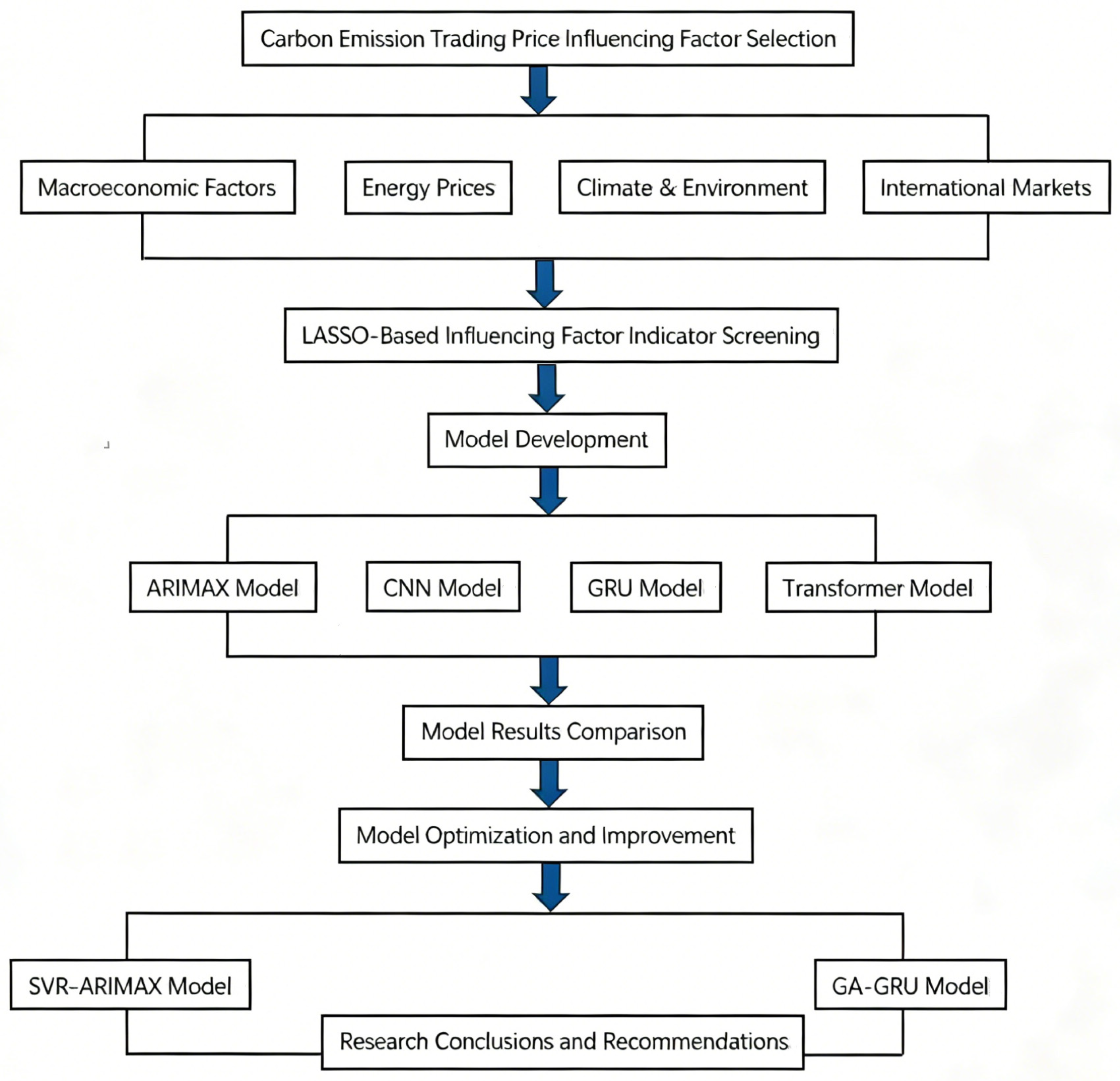
The dependent variable of this study is the average transaction price of carbon emission rights, defined as the ratio of the total transaction volume to the total transaction quantity of carbon emission allowances traded monthly in the five major carbon markets (Shenzhen, Guangdong, Hubei, Beijing, and Shanghai). Building on existing research, the indicators influencing this average price are categorized into four dimensions: macroeconomy, energy prices, climate and environment, and international markets. Details are presented in

Table 1. Details of the Indicator System.

Dimension	Indicator Name	Variable Code	Data Source
Dependent Variable	Carbon Emission Allowance Trading Average Price	$\mathrm{y}$	Sichuan United Environment Exchange
Macroeconomic	Consumer Price Index (CPI)	${\mathrm{x}}_1$	National Bureau of Statistics
	Producer Price Index for Industrial Products (PPI)	${\mathrm{x}}_2$	National Bureau of Statistics
	Trade Balance	${\mathrm{x}}_3$	National Bureau of Statistics
	Foreign Exchange Reserves	${\mathrm{x}}_4$	National Bureau of Statistics
Energy Prices	WTI Crude Oil Closing Price	${\mathrm{x}}_5$	Sina Finance
	Natural Gas Futures Closing Price	${\mathrm{x}}_6$	Sina Finance
	Coking Coal Futures Closing Price	${\mathrm{x}}_7$	Sina Finance
Climate & Environment	Air Quality Index (AQI)	${\mathrm{x}}_8$	China Air Quality Online Monitoring and Analysis Platform
International Markets	Euro Exchange Rate	${\mathrm{x}}_9$	Gold.org
	US Dollar Exchange Rate	${\mathrm{x}}_{10}$	Gold.org
	EUA Futures Closing Price	${\mathrm{x}}_{11}$	Sina Finance

:

4.3. Data Preprocessing and Influencing Factor Indicator Selection

This study selects relevant data from China’s five major carbon markets (Shenzhen, Guangdong, Hubei, Beijing, and Shanghai) spanning the period 2018–2024 for empirical analysis to verify the accuracy of the proposed models. It aims to provide a novel method for predicting the average transaction price of carbon trading, enhance prediction precision, and furnish forward-looking price forecasting information for market participants and policymakers. This support facilitates the formulation of scientific decisions and mitigates market risks.

To screen the factors influencing the average transaction price of carbon emission rights, the LASSO algorithm is employed for feature selection. First, the original data is divided into a training set and a test set, and all subsequent preprocessing and feature selection steps are performed only on the training set. Due to significant differences in the dimensions and orders of magnitude among the original data indicators, the data are first subjected to standardization processing: Normal distribution data are standardized using Z-score normalization; non-normal distribution data are normalized using min-max normalization. The normality of the data is assessed using the Shapiro–Wilk test (with p > 0.05 indicating a normal distribution), supplemented by Q-Q plots for verification [37]. Subsequently, 10-fold cross-validation is used to determine the λ value, with the goal of minimizing the cross-validation mean squared error (MSE) to find the λ value that achieves a bias-variance tradeoff for the model. Finally, the determined λ value is input into the LASSO model to select the key features.

Based on the LASSO regression, the insignificant influencing factors for each carbon market (i.e., those with a LASSO coefficient of 0) are screened out. The indicator selection results of the five carbon markets (Shenzhen, Guangdong, Hubei, Beijing, and Shanghai) are summarized, and the findings are presented in

Table 2. Results of Feature Screening Based on LASSO.

Feature Name	Significance	Shenzhen	Guangdong	Hubei	Beijing	Shanghai
Consumer Price Index (CPI)	Significant	Yes	No	Yes	Yes	Yes
	Lag Order	26		15	29	2
Producer Price Index (PPI)	Significant	No	Yes	Yes	No	Yes
	Lag Order		12	30		22
Trade Balance	Significant	Yes	No	No	Yes	Yes
	Lag Order	11			13	23
Foreign Exchange Reserves	Significant	No	No	No	No	No
	Lag Order
WTI Crude Oil Closing Price	Significant	Yes	Yes	Yes	Yes	Yes
	Lag Order	13	0	4	11	13
Natural Gas Futures Closing Price	Significant	Yes	Yes	Yes	No	Yes
	Lag Order	20	8	7		22
Coking Coal Futures Closing Price	Significant	No	Yes	Yes	Yes	Yes
	Lag Order		13	7	16	26
Air Quality Index (AQI)	Significant	Yes	Yes	Yes	Yes	No
	Lag Order	29	0	28	9
Euro to US Dollar Exchange Rate (EUR/USD)	Significant	Yes	No	No	Yes	Yes
	Lag Order	16			16	23
US Dollar Index (DXY) or Broad Dollar Exchange Rate	Significant	No	No	No	Yes	No
	Lag Order				1
EUA Futures Closing Price	Significant	Yes	Yes	Yes	Yes	Yes
	Lag Order	13	2	2	12	12

.

Through LASSO regression, the optimal lag orders of exogenous variables affecting carbon prices are identified. The analysis shows that the significant exogenous variables have lagged effects on carbon prices. Therefore, when predicting carbon prices for 2025, only historical data of exogenous variables (already observed values) are needed, without relying on unknown exogenous variable data for 2025. This fully utilizes the delayed response characteristics of carbon prices to exogenous variables, making multi-step forecasting feasible in practical applications.

4.4. Comparison and Selection of Carbon Trading Price Forecasting Models

To ensure the objectivity and scientific validity of model comparisons, this study establishes unified experimental conditions. All experiments were conducted using Python 3.13.5 on Windows 11 (64-bit, AMD64). Monthly average carbon trading price data from five major carbon markets spanning January 2018 to December 2024 are selected as the sample. The Expanding Window evaluation strategy is adopted, with the initial training set comprising 50% of the total sample. Subsequently, the window expands by one time point at each iteration, and the model is retrained using all available historical data to predict the next time point, resulting in a total of N rolling predictions (where N is the sample size of the test set). Three core evaluation metrics are employed: Root Mean Square Error (RMSE), Mean Absolute Error (MAE), and Mean Absolute Percentage Error (MAPE).

Additionally, prediction trend plots and 95% confidence intervals are provided. The confidence intervals are estimated using the Bootstrap method with 1000 resampling iterations, taking the 2.5th and 97.5th percentiles as the lower and upper bounds, respectively. Based on these settings, the adaptability of each model across different markets is comprehensively evaluated. The specific implementation and comparison results of each model are presented as follows.

(1)

Prediction Accuracy of the ARIMAX-Based Carbon Allowance Transaction Price Model

Taking the Hubei carbon market as an example, in the analysis of time series data, the Augmented Dickey–Fuller (ADF) test is first performed for stationarity verification. The results indicate that all original sequences are non-stationary except for the “Air Quality Index (AQI)” sequence, and all become stationary after first-order differencing (d = 1). Subsequently, combined with the autocorrelation and partial autocorrelation plots of ∇yt, the ARIMAX model is established using Python with repeated order determination and verification. The optimal model is identified as ARIMAX(2, 0, 2) based on the Bayesian Information Criterion (BIC) minimization principle. Finally, validation is conducted through model residual plots and the Ljung–Box test (statistic = 9.767124, p-value = 0.461157), leading to the conclusion that the residuals exhibit no autocorrelation, the model can fully extract time series information, and both the fitting and prediction performances are favorable.

The ARIMAX model specifications for the five markets show distinct differences. Shenzhen and Beijing adopt orders of (0, 0, 2) and (0, 0, 1), respectively, requiring no differencing and relying on moving average terms and residual corrections. Hubei adopts an order of (2, 0, 2), requiring no differencing while depending on both autoregressive and moving average terms. Guangdong is the only market requiring first-order differencing (d = 1), adopting an order of (0, 1, 1) and primarily relying on residual correction. Shanghai adopts an order of (1, 0, 0), requiring no differencing and depending solely on the autoregressive term. Regarding exogenous variables, the USD exchange rate has significant positive effects on Shenzhen and Beijing; CPI has significant negative effects on Shenzhen and Hubei; PPI and WTI crude oil price have significant effects only on Hubei; while all exogenous variables in Guangdong and Shanghai are not significant.

Based on the aforementioned methodology, the ARIMAX model fitting is performed separately for each of the five carbon markets, and the specific models corresponding to each market are presented in

Table 3. ARIMAX Model Specification for Each Carbon Market.

Carbon Markets	ARIMAX Model
Hubei	$\begin{array}{c}{y}_t-0.5653y_{t-1}+0.5444y_{t-2}\\ =\left(1+1.7386B-0.8266B^2\right){\epsilon }_t-0.1368{x1}_{1,t-15}\\ -0.9409{x2}_{1,t-30}+0.1428{x5}_{1,t-4}+0.0415\times {sigma2}_t\end{array}$
Beijing	$\begin{array}{c}{y}_t-y_{t-1}=-0.9589{\epsilon }_{t-1}+4.8198\times {X10}_t\\ -0.9589\times ma.{L1}_t+0.2874\times {sigma2}_t+{\epsilon }_t\end{array}$
Guangdong	$y_t-y_{t-1}=-0.9386{\epsilon }_{t-1}-0.9386\times ma.{L1}_t$ $+0.0357\times {sigma2}_t+{\epsilon }_t$
Shenzhen	$y_t-y_{t-1}=0.0604\times {sigma2}_t+{\epsilon }_t$
Shanghai	$y_t-0.472y_{t-1}=0.0197\times {sigma2}_t+{\epsilon }_t$

.

$a.L1$ denotes the first-order lag variable of the average carbon trading price; sigma 2 typically represents the variance of the error term; ${\epsilon }_t$ is the white noise error term; and ${\epsilon }_{t-1}$ denotes the first-order lag of the white noise error term.

The prediction graphs and 95% confidence intervals for the average transaction price of carbon trading in each market over the next 12 months, generated by the constructed ARIMAX model, are illustrated in Figure 2.

As illustrated in Figure 2, carbon prices across markets within the sample period exhibit synchronized cyclical fluctuation characteristics, characterized by low-level volatility in the early stage, a sustained upward surge following 2022, and a subsequent pullback from elevated levels in the later stage. The predicted curves generated by the model are able to closely align with the overall operational trends and short-term fluctuation rhythms of carbon prices across markets, with only minor deviations observed at extreme market turning points and peak prices during sharp rallies. The model demonstrates robust fitting performance and favorable cross-market adaptability with respect to carbon price trajectories across different regions.

(2)

Carbon Allowance Transaction Price Prediction Based on the CNN Model

The parameters of the CNN model in this study were set as follows:

Table 4. Parameter Configuration of the CNN Model.

Convolutional Layer			Fully Connected Layer 1		Fully Connected Layer 2
Input Channels	Output Channels	Kernel Size	Input Dim	Output Dim	Input Dim	Output Dim
8	64	1	64	32	32	1

presents the parameter settings of the CNN model. The convolutional layer has 8 input channels (corresponding to the 8 feature variables) and 64 output channels with a kernel size of 1, capturing contemporaneous correlations among features. The first fully connected layer compresses the 64-dimensional features to 32 dimensions to learn high-order nonlinear combinations; the second fully connected layer maps the 32-dimensional features to a 1-dimensional predicted value.

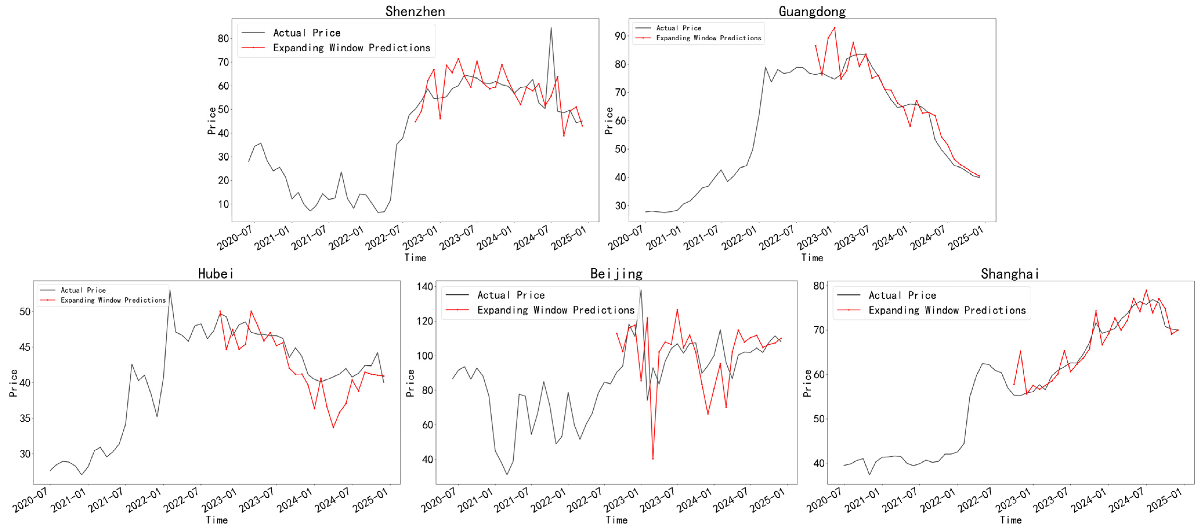
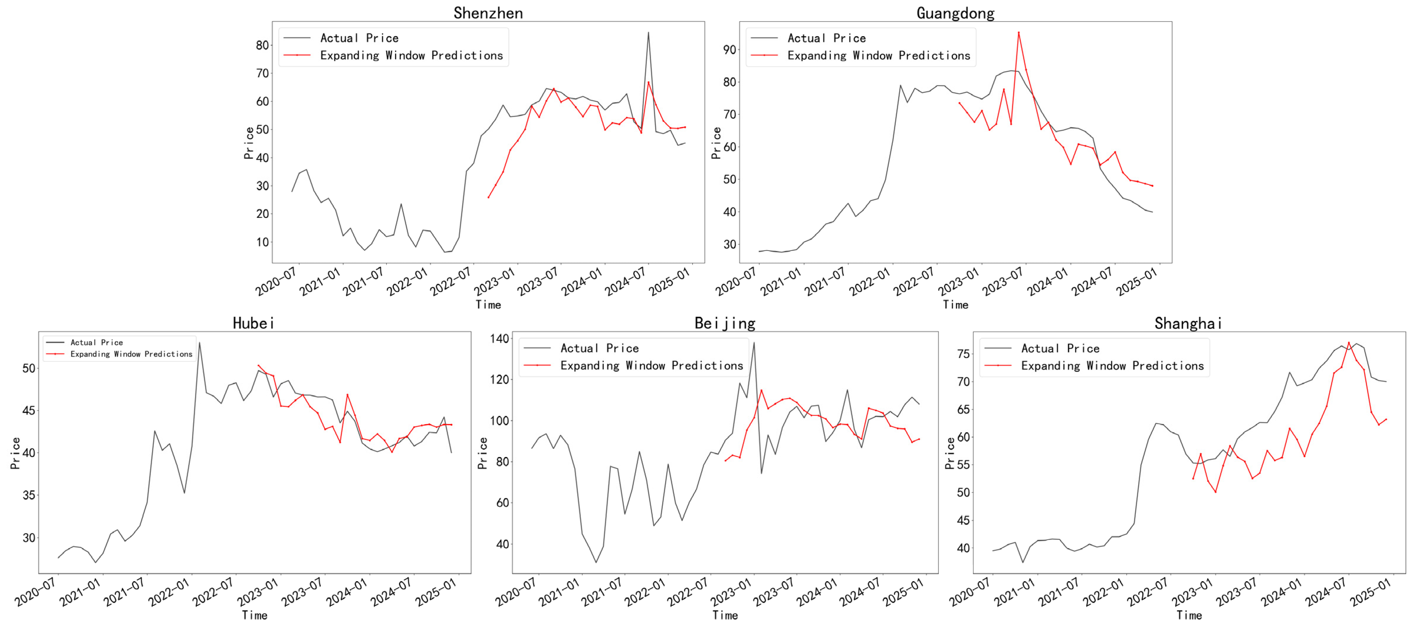
As illustrated in Figure 3, carbon price trajectories across markets within the sample period exhibit a high degree of synchronization, each undergoing a complete cycle characterized by low-level volatility in the early stage, a sustained upward surge following 2022, and a subsequent pullback from elevated levels commencing at the end of 2023. Both types of window models are able to closely follow the operational trends and fluctuation rhythms of carbon prices across markets, with only minor prediction deviations observed at the peak positions of extreme price spikes. The models demonstrate a pronounced capability for identifying market turning points. Overall, the fitting performance is robust, and the models exhibit favorable adaptability across diverse carbon market environments.

(3)

Carbon Allowance Transaction Price Prediction Based on the GRU Model

The parameters of the GRU model in this study were set as follows:

Table 5. Parameter Configuration of the GRU Model for Carbon Allowance Transaction Price Prediction.

Input Size	Output Size	Timesteps	Batch Size
50	1	1	32

presents the parameter settings of the GRU model. The input size is 50, indicating that the model processes 50 time steps of historical sequence data at each iteration. The output size is 1, meaning the model predicts the carbon price at the next time point. The timestep is 1, indicating that the model considers only the input features of a single time point for prediction at each step. The batch size is 32, meaning the model processes 32 samples simultaneously in each training iteration.

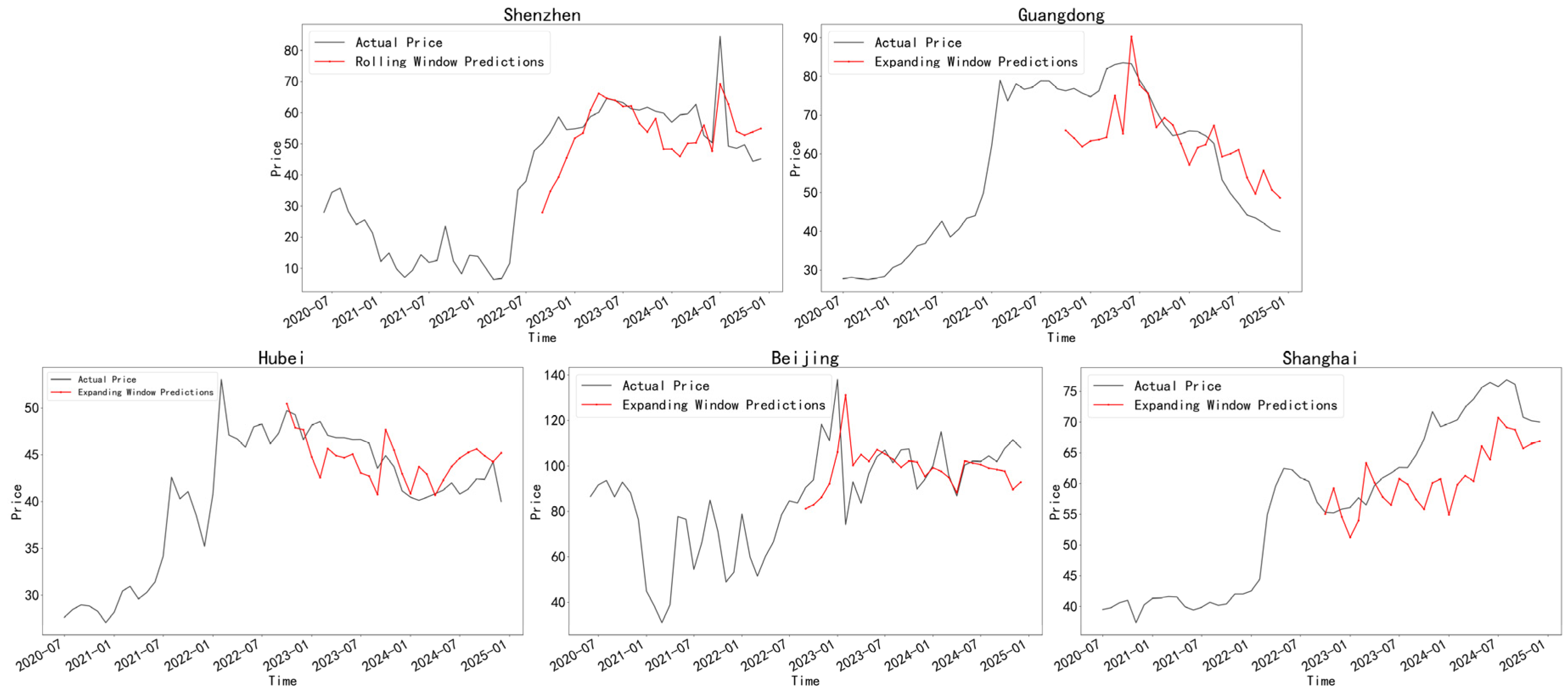
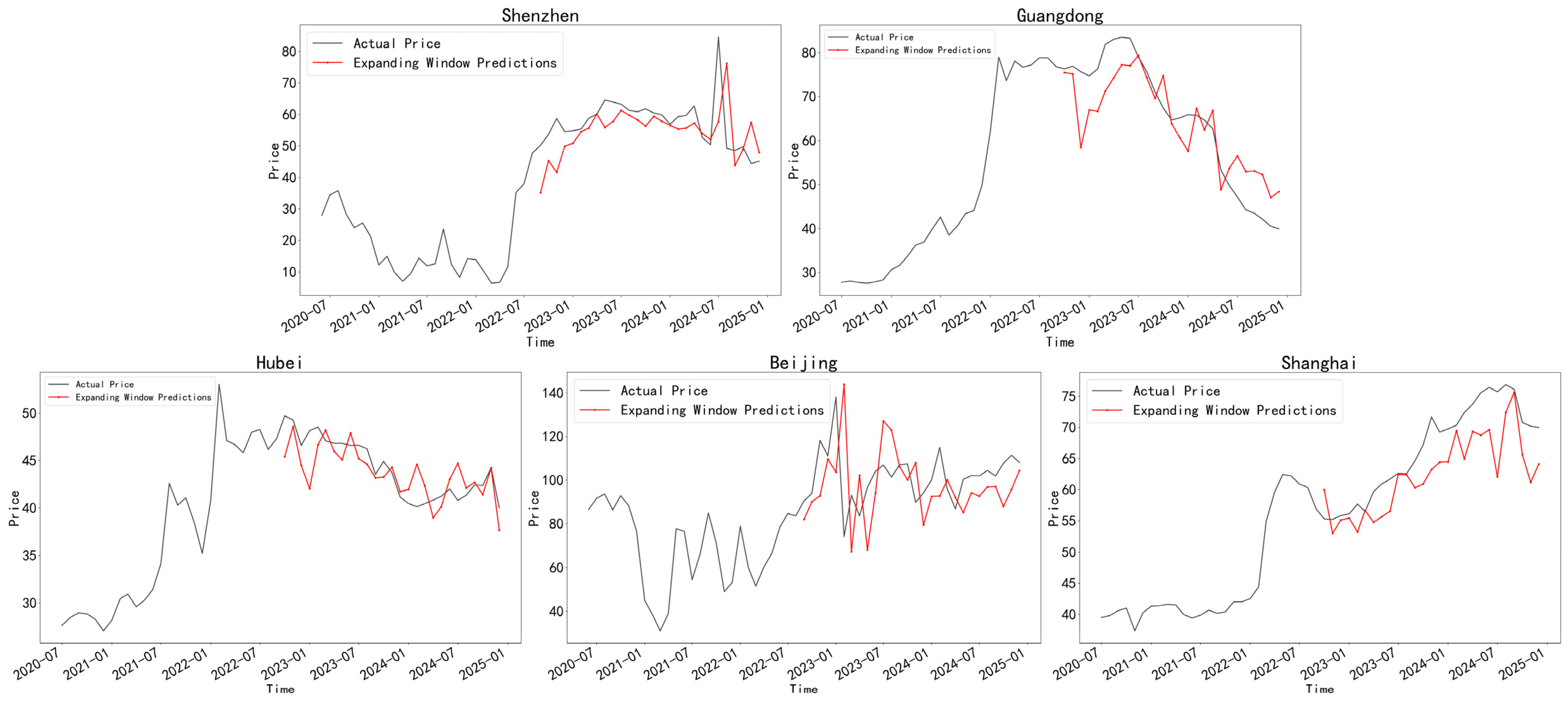
As illustrated in Figure 4, carbon prices across markets exhibit a synchronized cyclical trajectory characterized by low-level volatility in the early stage, a sustained upward surge following 2022, and a subsequent pullback from elevated levels commencing at the end of 2023. The predicted curves generated by the model are able to closely align with the overall operational trends and fluctuation rhythms of carbon prices in each market, with only a slight overestimation bias observed at the peak nodes of extreme price spikes. The model demonstrates a pronounced capability for identifying market turning points. Overall, the fitting performance is robust, and the model exhibits favorable adaptability across diverse carbon markets.

(4)

Carbon Allowance Transaction Price Prediction Based on the Transformer Model

The parameters of the Transformer model were configured as follows:

Table 6. Parameter Configuration of the Transformer Model for Carbon Allowance Transaction Price Prediction.

Input Dimension	Feature Dimension	Number of Attention Heads	Encoder Layers	Output Dimension
Number of Features in the Training Data	64	4	2	1

presents the parameter configuration of the Transformer model for carbon allowance transaction price prediction. The input dimension is the number of features in the training data (8 features). The feature dimension is 64, used for embedding mapping. The number of attention heads is 4, enabling parallel capture of feature relationships. The number of encoder layers is 2, enhancing feature extraction capability. The output dimension is 1, producing the predicted carbon price.

As illustrated in Figure 5, carbon price trajectories across markets exhibit a generally convergent pattern over the sample period, each undergoing a complete cycle characterized by low-level volatility in the early stage, a sustained upward surge following 2022, and a subsequent pullback from elevated levels after late 2023. The predicted curves generated by the model are able to closely follow the fluctuation patterns and overall trends of carbon prices in each market, with only a slight overestimation bias observed at the peak nodes of extreme price spikes. Overall, the model demonstrates robust fitting performance and favorable cross-market adaptability.

(5)

Comparative Evaluation of Testing Accuracy for Carbon Allowance Transaction Price Prediction

This study selects the Root Mean Square Error (RMSE) as the primary evaluation metric based on valid theoretical and methodological grounds. To provide a more comprehensive assessment of model performance, the Mean Absolute Error (MAE) and the Mean Absolute Percentage Error (MAPE) are also adopted. The test precision of each model with respect to these three metrics is presented in

Table 7. Comparison of Metrics Across Different Models in Five Carbon Markets.

Market	Metric	ARIMAX	GRU	CNN	Transformer
Shenzhen	RMSE	8.7342	10.0167	9.8973	9.4750
	MAE	6.3401	7.2467	7.7672	6.2383
	MAPE	10.8993%	12.8216%	13.9056%	10.9482%
Guangdong	RMSE	5.7488	7.7673	9.6141	7.2114
	MAE	3.7704	6.6215	8.2547	6.0184
	MAPE	5.6896%	10.7906%	13.6101%	10.2084%
Hubei	RMSE	2.9634	1.8553	2.7763	2.2245
	MAE	2.3731	1.5224	2.3690	1.7223
	MAPE	5.4502%	3.4463%	5.4038%	3.8980%
Beijing	RMSE	20.8844	16.1509	16.7008	20.6060
	MAE	14.9255	11.9813	10.9729	15.4413
	MAPE	15.3520%	11.9451%	11.1444%	15.9012%
Shanghai	RMSE	2.7671	7.0665	7.7234	5.5315
	MAE	2.0356	6.2716	6.5566	4.5558
	MAPE	3.1364%	9.3781%	9.5366%	6.6644%

.

According to the RMSE, MAE, and MAPE results across the five markets, ARIMAX and GRU are the top two models. ARIMAX performs best in Shenzhen, Guangdong, and Shanghai with minimal errors, while GRU excels in Hubei and Beijing, significantly outperforming CNN and Transformer in error control. The fundamental reason for this performance gap lies in the difference in temporal dependency modeling capabilities. ARIMAX and GRU possess recursive states or autoregressive components, making them naturally suitable for capturing the strong autocorrelation of carbon price series. In contrast, CNN and Transformer are “feed-forward” models that lack the ability to model temporal dependencies. In the small-sample, one-step-ahead rolling window forecasting scenario, recursive models (ARIMAX/GRU) have higher parameter efficiency and better match the data characteristics, thus achieving superior performance.

4.5. Carbon Allowance Price Prediction Based on Optimized ARIMAX and GRU Models

Multiple optimization algorithms were tested, and the following two were found to be the most appropriate for this study.

(1)

Improved ARIMAX Model and Its Prediction

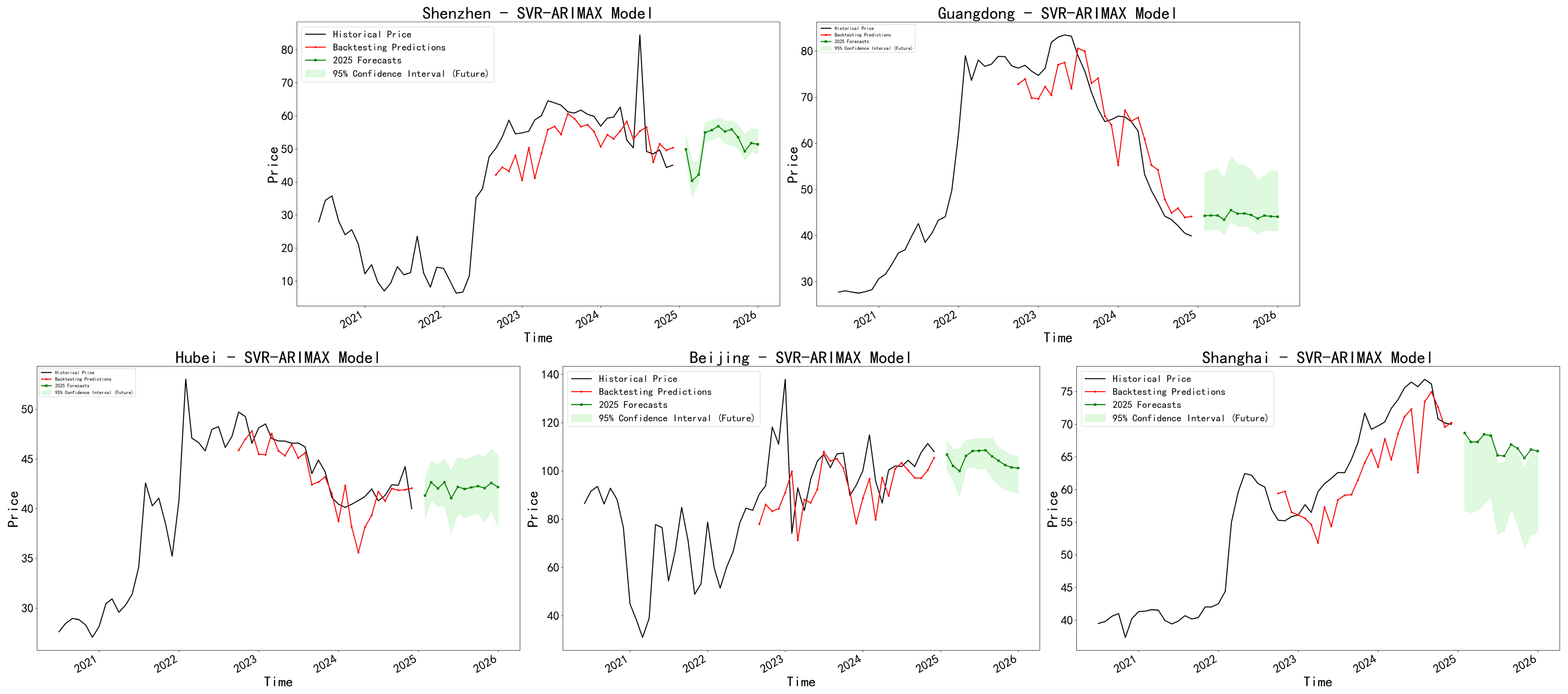
We apply the SVR-ARIMAX model to the carbon markets, and the obtained prediction results are presented in Figure 6:

Based on a comparative analysis of the RMSE, MAE, and MAPE metrics across the five markets—Shenzhen, Guangdong, Hubei, Beijing, and Shanghai—the SVR-ARIMAX model achieves significant improvements over the baseline ARIMAX in the majority of markets (

Table 8. Comparison of Metrics Across ARIMAX and SVR-ARIMAX in Five Carbon Markets.

Market	Metric	ARIMAX	SVR-ARIMAX
Shenzhen	RMSE	8.7342	9.4949
	MAE	6.3401	7.5566
	MAPE	10.8993%	12.7808%
Guangdong	RMSE	5.7488	5.5139
	MAE	3.7704	3.6212
	MAPE	5.6896%	4.3074%
Hubei	RMSE	2.9634	2.0948
	MAE	2.3731	1.7174
	MAPE	5.4502%	3.9088%
Beijing	RMSE	20.8844	16.1214
	MAE	14.9255	11.9492
	MAPE	15.3520%	11.5971%
Shanghai	RMSE	2.7671	5.0620
	MAE	2.0356	4.1606
	MAPE	3.1364%	6.2128%

). Specifically, SVR-ARIMAX yields lower error values across all three metrics in Guangdong, Hubei, and Beijing, with the most pronounced enhancement observed in the Beijing market (RMSE decreasing from 20.8844 to 16.1214, MAPE decreasing from 15.35% to 11.60%) and substantial improvements also evident in the Hubei market (RMSE decreasing from 2.9634 to 2.0948). However, in the Shenzhen and Shanghai markets, SVR-ARIMAX exhibits higher error metrics compared to ARIMAX, with particularly inferior performance relative to the benchmark model in the Shanghai market.

According to the long-term price forecasting results of five Chinese carbon emission trading pilots (Shenzhen, Guangdong, Hubei, Beijing and Shanghai) based on the SVR-ARIMAX model, the historical carbon prices of all markets have undergone a complete operational cycle consisting of low-level accumulation, medium-term sharp rally, and subsequent corrective decline. The in-sample backtesting curve of the model achieves favorable fitting performance in capturing the historical trend and volatility characteristics of carbon prices. In view of the green long-term forecasting curves from 2025 to 2026 and their corresponding 95% confidence intervals, distinct clustered operational patterns are identified among the five markets. Specifically, the two South China markets, Shenzhen and Guangdong, exhibit highly consistent future trajectories: following prior adjustments, Shenzhen will complete a short-term bottom probing and subsequently enter an oscillatory recovery channel, and its moderately wide confidence interval indicates controllable overall uncertainty of future price movements. After profound prior corrections, Guangdong will step into a long-term horizontal consolidation phase; its stable green forecasting curve and moderately broad confidence interval demonstrate weak future price volatility and predominant range-bound operation. The two core markets of Beijing and Hubei share analogous future trend characteristics. Supported by their historically high price benchmarks, both markets present trajectories of narrow oscillatory decline and gradual bottom consolidation within the forecasting horizon, with medium-width confidence intervals signifying mild long-term price adjustment and manageable overall volatility risks. As for the Shanghai market, it features a relatively independent evolution trend. After peaking in the early stage, it will maintain a slow downward trajectory in the future. Meanwhile, its confidence interval is notably wider than that of other pilots, which reflects remarkable long-term downward pressure and relatively higher uncertainty in future price fluctuations.

(2)

Improved GRU Model and Its Prediction

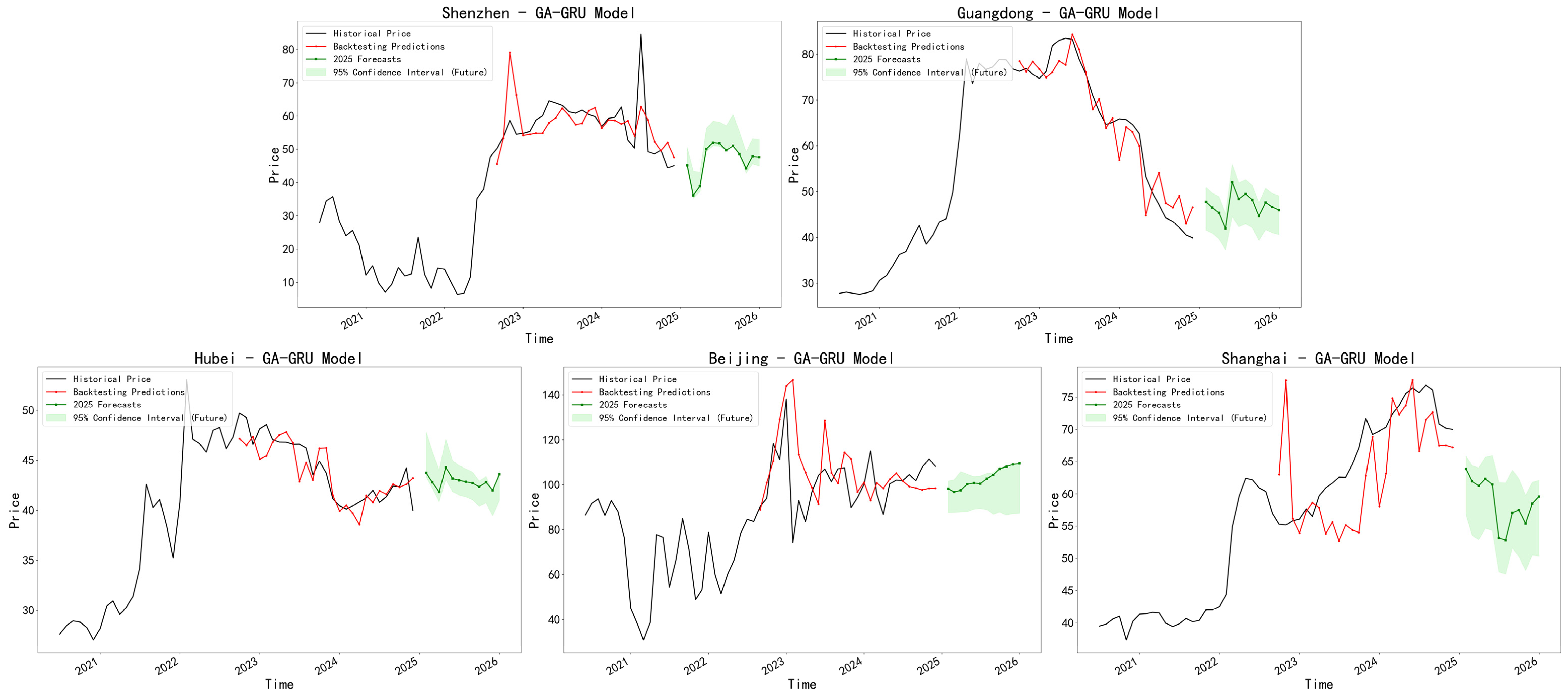
We apply the GA-GRU model to the carbon markets, and the corresponding prediction results are presented in Figure 7:

As shown in

Table 9. Comparison of Metrics Across GRU and GA-GRU in Five Carbon Markets.

Market	Metric	GRU	GA-GRU
Shenzhen	RMSE	10.0167	7.1672
	MAE	7.2467	4.7739
	MAPE	12.8216%	8.1509%
Guangdong	RMSE	7.7673	4.1427
	MAE	6.6215	3.3285
	MAPE	10.7906%	5.7722%
Hubei	RMSE	1.8553	1.7436
	MAE	1.5224	1.3390
	MAPE	3.4463%	2.9800%
Beijing	RMSE	16.1509	17.7925
	MAE	11.9813	11.3704
	MAPE	11.9451%	12.8167%
Shanghai	RMSE	7.0665	6.5113
	MAE	6.2716	5.6538
	MAPE	9.3781%	8.7546%

, based on a comparative analysis of the RMSE, MAE, and MAPE metrics across the five markets—Shenzhen, Guangdong, Hubei, Shanghai, and Beijing—the GA-GRU model demonstrates substantial improvements over the standard GRU in the majority of markets. Specifically, GA-GRU achieves lower error values across all three metrics in Shenzhen, Guangdong, Hubei, and Shanghai, with the most pronounced enhancement observed in the Guangdong market, where RMSE decreases from 7.7673 to 4.1427 and MAPE declines from 10.79% to 5.77%. Steady improvements are also evident in the Hubei market. In contrast, within the Beijing market, GA-GRU yields marginally higher RMSE and MAPE values relative to GRU, suggesting that the optimization algorithm’s adaptability to extremely volatile market conditions remains subject to further refinement. Overall, the genetic algorithm-based parameter optimization of GRU effectively reduces prediction errors across most regional carbon markets, thereby enhancing model fitting accuracy and robustness.

According to the long-term price forecasting results of five domestic carbon emission trading pilots (Shenzhen, Guangdong, Hubei, Beijing and Shanghai) based on the GA-GRU model, all markets have undergone a complete operational cycle consisting of low-level consolidation, mid-term volatile rally, and subsequent corrective adjustment in historical carbon price movements. The in-sample backtesting results of the model demonstrate favorable fitting performance, with strong capability in capturing historical price trends and volatility inflection points. In light of the 2025–2026 green long-term forecasting curves and their corresponding 95% confidence intervals, distinct clustered operational patterns are identified across the five markets. The two South China markets, Shenzhen and Guangdong, exhibit highly consistent future trajectories: both will achieve bottom stabilization following prior corrections, followed by moderate oscillatory upward movements. Their moderately narrow confidence intervals indicate low future price volatility risks, signaling a steady recovery trajectory ahead. The two core markets of Beijing and Hubei share analogous trend characteristics; resting on their historically high price benchmarks, they will maintain slow incremental growth within narrow volatility bands. Their compact confidence intervals reflect the strongest price stability among all pilots, with robust long-term price support fundamentals. As for the Shanghai market, it features a relatively independent dynamic, presenting a typical pattern of initial mild downside correction succeeded by volatile rebound and upward recovery. Its comparatively wider confidence interval than other pilots denotes explicit upward recovery potential alongside relatively elevated short-term uncertainty in price fluctuations. On the whole, all five pilot carbon markets will terminate their prior unilateral downward adjustment after 2025, collectively stepping into a new phase of stabilization, recovery and gradual upward elevation of price benchmarks. Heterogeneities in recovery pace and volatility amplitude merely arise from inherent regional market differentiation, while the reasonable coverage of overall forecasting intervals verifies the high reliability of the model’s projections on future carbon price dynamics.

5. Conclusions and Future Work

This study employs the LASSO algorithm to screen influencing factors from four dimensions and identifies the key factors and their optimal lag orders for carbon prices across five major carbon markets. The results show that, despite variations across markets, “WTI crude oil price” and “EUA futures closing price” are consistently significant factors in all five markets, reflecting the transmission effects of international energy price fluctuations and EU carbon market linkages on China’s carbon price formation, as well as the deep integration of domestic carbon markets into the global energy and climate governance system.

On this basis, this study constructs the ARIMAX time series model and machine learning models including CNN and GRU, using RMSE, MAE, and MAPE as evaluation metrics to analyze and predict average carbon trading prices. The results indicate significant differences in prediction accuracy across models: ARIMAX performs better in Guangdong and Shanghai, while GRU excels in Shenzhen, Hubei, and Beijing. To address the limitations of the better-performing ARIMAX and GRU models, this study introduces SVR and GA algorithms for optimization: SVR to construct the SVR-ARIMAX hybrid model, and GA to construct the GA-GRU hybrid optimization model. SVR-ARIMAX achieves significantly lower errors than the baseline ARIMAX in Beijing, Hubei, and Guangdong, with the most pronounced improvement in Beijing (RMSE decreasing from 20.8844 to 16.1214, MAPE from 15.35% to 11.60%). However, in Shenzhen and Shanghai, SVR-ARIMAX yields higher errors than ARIMAX. GA-GRU outperforms standard GRU in Shenzhen, Guangdong, Hubei, and Shanghai, with the most significant improvement in Guangdong (RMSE decreasing from 7.7673 to 4.1427, MAPE from 10.79% to 5.77%). In Beijing, GA-GRU yields slightly higher RMSE and MAPE than GRU, suggesting room for improvement in adapting to extreme market volatility.

Based on the 12-month-ahead forecasting results, the volatility characteristics of carbon prices are closely related to the transmission speed of their influencing factors. In Guangdong, the WTI Crude Oil Closing Price and the Air Quality Index exhibit contemporaneous transmission, coupled with medium- and short-term lagged factors such as the Natural Gas Futures Closing Price and the Coking Coal Futures Closing Price, enabling the market to absorb external shocks efficiently and adjust prices fully, thus achieving the most stable trajectory. In Hubei, key factors including the Producer Price Index, the Consumer Price Index, and the Air Quality Index all display long-lagged and dispersed transmission characteristics, allowing external shocks to be incorporated into prices in a slow and smooth manner, which endows carbon prices with strong resilience within a narrow range-bound fluctuation. In Beijing, the generally long lag orders of variables such as the Consumer Price Index, the EUA Futures Closing Price, the Trade Balance, the WTI Crude Oil Closing Price, the Euro to US Dollar Exchange Rate, and the US Dollar Index indicate an expectation-driven market mechanism, where participants digest and price in information well before its full realization, ultimately driving carbon prices toward stable convergence at a high level. In Shanghai, the Consumer Price Index exhibits short-term rapid response, while the Coking Coal Futures Closing Price, the Natural Gas Futures Closing Price, the Producer Price Index, and the Trade Balance show long-term slow absorption; this mixed fast-slow transmission mechanism implies considerable upside resilience beneath the surface of apparent stability, leading to higher forecasting uncertainty. In Shenzhen, almost all significant factors—including the Consumer Price Index, the Air Quality Index, the Trade Balance, the WTI Crude Oil Closing Price, the EUA Futures Closing Price, the Natural Gas Futures Closing Price, and the Euro to US Dollar Exchange Rate—are characterized by medium- to long-term lags, forming a pronounced slow-transmission accumulation effect. External shocks accumulate over extended periods and are released in a concentrated manner, resulting in the highest volatility and forecasting uncertainty among the five markets.

This study offers methodological references for predicting carbon allowance trading prices across multiple markets through multi-model comparison. Compared with previous studies, it not only validates the mainstream conclusions that energy prices, international carbon markets, and macroeconomic conditions significantly affect carbon prices, but also reveals regional heterogeneity through cross-pilot comparisons, addressing the gap in existing literature that mostly focuses on single markets. Meanwhile, the hybrid optimization models outperform single models in prediction accuracy, consistent with mainstream hybrid forecasting approaches and better suited to China’s pilot carbon markets.

However, this study has several limitations. First, only five pilot markets are selected without incorporating national carbon market data, limiting the representativeness of the conclusions. Second, only monthly low-frequency data are used, failing to capture intraday and short-term high-frequency volatility. Third, the optimization algorithm shows limited effectiveness in certain markets, and the compatibility between algorithms and models requires further improvement.

Future research can incorporate high-frequency trading data and policy dummy variables to build a prediction framework integrating external shocks, combine prediction models with risk warning and carbon asset pricing to expand application scenarios, and conduct comparative studies between the national carbon market and pilot markets. In addition, multi-objective optimization and ensemble learning methods can be explored to further improve model stability and generalization capability in highly volatile markets.