Walking, Jogging, and Cycling: What Differs? Explainable Machine Learning Reveals Differential Responses of Outdoor Activities to Built Environment

Abstract

The development of street-based outdoor physical activities plays a vital role in improving public health issues and advancing the goals of the “Healthy China” initiative, and the built environment is widely considered a key factor in promoting such activities and urban sustainability. Existing studies have paid limited attention to the nonlinear relationships between the built environment and outdoor physical activity and have mostly focused on a single type of activity (such as walking or cycling), with few comparative analyses across different activity types. With the purpose of addressing these limitations and providing cross-sectional empirical evidence for sustainable street design and active-transport policy, this study examines streets within the Second Ring Road of Changsha and uses large-scale street-level outdoor activity trajectory data to investigate associations between built environment indicators and outdoor activity flows. A Random Forest model, followed by the application of SHapley Additive exPlanations (SHAP), is used to characterize the nonlinear associations and interactions among variables, capturing patterns relevant to sustainable mobility, public health and urban form. The results indicate the following: (1) The built environment indicators are associated with walking, jogging, and cycling in distinctly different patterns—walking shows stronger associations with population density and access to bus stops; jogging demonstrates stronger associations with the accessibility of large open spaces; and cycling is more associated with land use mix and road intersection density. (2) Nonlinear associations and threshold-like patterns commonly exist between built environment variables and activity flows, with indicators such as bus stop density and walking continuity exhibiting pronounced effects within specific intervals. (3) Interaction effects among variables contribute importantly to model predictions, especially for jogging where their influence can even exceed the main effects of individual factors. These results underscore the potential value of implementing tailored street design strategies for different activity types and provide empirical evidence relevant to health-oriented urban planning.

1. Introduction

Public health is a perennial concern for human societies, and numerous studies indicate that insufficient physical activity is a major contributor to most chronic diseases, including heart disease, hypertension, and obesity [1,2]. At the same time, recent research indicates that accruing more steps per day is associated with steady declines in dementia incidence risk, with the maximal observed benefit occurring at approximately 9800 steps per day [3]. According to a recent systematic review and meta-analysis, active commuting (such as walking and cycling) is significantly associated with a reduced risk of type 2 diabetes, with active commuters showing an approximately 19% lower risk compared to non-active commuters [4], and a recent large-scale meta-analysis confirmed that physical activity interventions, including walking and jogging, serve as effective treatments for depression, often comparable to psychotherapy or pharmacotherapy [5]. Therefore, promoting routine outdoor physical activity has become a key objective for governments and urban planners, and is important for reducing disease incidence and improving population health.

Domestic and international scholars have conducted studies on how to increase residents’ willingness to participate in outdoor physical activity and how to promote such activity. They found that streets, as important settings for daily commuting and leisure, have built environment characteristics that substantially influence residents’ outdoor activity levels and, consequently, their health [6]. A large body of empirical research shows that factors such as the spatial structure of the street built environment, transport facilities, green-space coverage, and land use types significantly affect residents’ physical activity behaviors: A higher degree of land use mix is associated with more active walking behavior among residents [7]. High green-space coverage and well-developed pedestrian infrastructure significantly increase residents’ willingness to walk [8]. In studies of jogging behavior, researchers further note that a dense road network provides runners with diverse route options and increases residents’ propensity to engage in outdoor activity [9]. Quality green landscapes not only offer safe and comfortable spaces for jogging, but also improve runners’ mental well-being [10]. Research on cycling behavior indicates that factors such as the road width, number of lanes, traffic volume, traffic safety facilities, and slope jointly determine the feasibility and comfort of cycling [11].

However, three principal limitations still persist in the current research in this field. First, previous studies have mainly relied on traditional survey data or two-dimensional planar data to measure the built environment, often overlooking the three-dimensional perceptual quality of streets that residents experience first-hand, which can lead to a disconnect between research metrics and residents’ lived experience. Second, although statistical models such as multiple linear regression can identify linear associations, they cannot capture the complex nonlinear relationships and interaction effects that may exist between the built environment and activity flows [12]. Finally—and critically—the existing literature often concentrates on the influence of built environment factors on a single activity type, lacking comparative studies that juxtapose different activity types [11]. Different activity types show clear differences in speed, distance, and environmental perception, and their relationships with the built environment may therefore be markedly heterogeneous. Ignoring this heterogeneity limits a comprehensive understanding of the field; hinders accurate elucidation of the complex, multidimensional mechanisms linking residents’ outdoor activities to the built environment; and impedes the formulation of targeted planning recommendations.

This study focuses on urban areas within the Second Ring Road of Changsha in China. We aimed to fill the aforementioned gaps by constructing an integrated analytical framework. Trajectory data for walking, jogging, and cycling and perception data derived from Street View Images (SVIs), point-of-interest (POI) data, and other urban morphological datasets were integrated into the study. The aims of our study were as follows: (1) Analyze the spatiotemporal characteristics of walking, jogging, and cycling within the Second Ring Road of Changsha. (2) Construct a multidimensional set of built environment indicators encompassing attractiveness, vitality, and accessibility. (3) Employ Random Forest regression models to examine the associations between built environment variables and the flows of the three activity types. (4) Apply SHapley Additive exPlanations (SHAP) to interpret the Random Forest outputs and explicitly reveal the nonlinear relationships and interaction effects among built environment factors influencing each activity type.

2. Literature Review

2.1. Research History of Healthy Streets

The topic of “healthy streets” originated in public-health research and has gradually matured through practice in urban design and transport policy. In 1996, the U.S. Centers for Disease Control and Prevention published a report on the relationship between health and physical activity [13]; thereafter, public health research began to focus on the links between chronic diseases, mortality, and insufficient outdoor physical activity. At that stage, research on physical activity remained focused on individual-level epidemiological controls and lacked a connection to urban space and the built environment. The consequent challenges of population aging, environmental change, and shifting lifestyles since the turn of the 21st century have driven an increase in research linking physical activity with the urban built environment and an evolution in this field from theoretical academic inquiry into concrete policy and institutional practice. In 2010, the New York City government introduced Active design guidelines: Promoting physical activity and health in design, which framed urban design around public health objectives [14]. In 2019, Ramirez-Rubio et al. [15] employed the Health in All Policies (HiAP) approach to explore links between urban policy and physical activity, providing guidance for governments seeking to mainstream activity promotion into policy.

China has also long explored the relationship between health and the built environment. In 1990, Weng et al. [16] noted that environmental factors, including the natural, built, and social environments, affect people’s physical-activity behaviors. In 1992, Chen [17] conducted the project A Literature Review: A Collaborative Study on Housing Type, Environment, and Residents’ Health, investigating associations between health and the built environment. In 2005, Liu et al. [18] published in New Architecture an overview of the U.S. “Active Design” initiative, including its background, interventions, and lessons learned, which introduced the concept of environmental impacts on health into China. Subsequently, Lv et al. [19], Zhu et al. [20], and Dong et al. [21] successively introduced theories such as healthy urban space design and the social–ecological model into the domestic discourse. By this point, qualitative research on “healthy streets” in China had matured. In 2016, the State Council of the PRC issued the Outline of the Healthy China 2030 Plan and advocated for the construction of healthy cities [22], signaling that China formally integrated the linkage between physical activity and urban space into urban design and national policy and began broad implementation. With the development of big data and artificial intelligence, data types have become more diverse and research methods and techniques more advanced, and China’s analysis of the Healthy Street Approach has progressively entered a phase dominated by quantitative analysis. Yu et al. [23] described the spatiotemporal dynamics of residents’ street-based fitness activities using data from fitness mobile apps and analyzed activity hotspots across three dimensions—spatial aggregation, the built environment, and population income. Zhao et al. [24] identified built environment characteristics that influence physical activity based on spatial distribution patterns of green space physical activity.

2.2. Measurement of PA

In quantitative studies of outdoor physical activity, trajectory data are a commonly used data source. Trajectory data consist of timestamped sequences of locations and typically include attributes such as the spatial coordinates of sample points, sampling times, and speed [25]. Common methods for collecting trajectory data include handheld Global Positioning System (GPS) receivers, mobile phone data, public transport smart-card records, and volunteered geographic information (VGI). Data collected by GPS devices are characterized by high temporal and spatial density and high positional accuracy but typically small sample sizes; such trajectories are often obtained by having volunteers wear GPS devices during activities. For example, Alberico et al. [26] combined waist-worn accelerometers (ActiGraph) with QStarz GPS units to record seven days of physical activity in children aged 5–10 and quantified the proportion of moderate-to-vigorous physical activity occurring in parks and playgrounds. Mobile phone data enable the collection of very large samples but offer lower spatial precision, tracking trajectories by recording signal or cell tower locations. For instance, Grantz et al. [27] used mobile phone data to monitor the effectiveness of nonpharmaceutical interventions against COVID-19, to assess potential spatiotemporal drivers of transmission, and to trace contacts. Public transport smart-card reports record passengers’ origin and destination stop locations and timestamps, thereby capturing passenger movement trajectories. Zhong et al. [28], for example, compared urban mobility patterns in London, Singapore, and Beijing using one week of public transport smart-card records. Although mobile phone data and public transport smart-card records can yield large volumes of trajectory data, both suffer from limited per-sample information content and lower spatial accuracy. Volunteered geographic information (VGI) refers to movement-related spatial data uploaded by users via applications on smart devices and is characterized by higher accuracy, greater spatiotemporal density, and richer per-sample information. Newzoo global mobile market report 2021 indicates that the number of smartphone users in China far exceeds that of other countries [29]. Leveraging this sampling advantage, Chinese researchers have extensively used VGI to investigate users’ outdoor activity patterns. Meng studied mountain fitness trails by extracting user-uploaded route trajectories from fitness apps and analyzed trail usage patterns, landscape preferences, and spatial experiences along the routes [30]. Ding validated actual usage of the Hangzhou greenway by scraping trajectory data from users of activity-tracking mobile applications [31]. When using the above trajectory data to study physical activity, researchers should attend to issues such as trajectory segmentation, the effects of sampling frequency on speed and behavior recognition, and privacy protection.

2.3. Nonlinear Associations Between Built Environment and PA

In recent years, quantitative research on the relationship between the built environment and outdoor activities has generally shifted from assuming linear relationships to utilizing machine learning methods that reveal nonlinear associations without predefined functional forms. Representative methodologies include GBDT, XGBoost, and Random Forest, followed by the use of interpretive tools such as PDP or SHAP to identify thresholds and local effects. Early representative studies providing nonlinear evidence, such as those of Ding et al. [32], Tao et al. [33], and Wu et al. [34], demonstrated strong nonlinearity and effective ranges regarding the impact of the built environment on travel distance or walking accessibility.

The relationship between walking and the built environment remains the most extensively studied sub-field. Machine learning research indicates that spatial attributes, such as density, land use mix, road network connectivity, and distance to centers/stations, exert nonlinear marginal effects on walking distance and probability. These effects are sensitive within specific “effective ranges,” beyond which marginal impacts rapidly diminish or reverse. [35] Tao et al. [33] noted in their study on walking distance that variables such as land use diversity, population density, and employment density exhibit distinct effective ranges. Meanwhile, reviews and empirical studies focusing on the elderly show that in highly compact areas, additional increases in density do not always promote walking and may even yield negative effects [12]. This suggests that planning interventions must identify these thresholds rather than adhering to a “the denser, the better” approach. Research addressing cycling, particularly shared bike systems, is also increasingly adopting methods like Random Forest and XGBoost to capture nonlinearity and complex interactions. Zhou et al. [36] utilized the Random Forest model to analyze the choice between Bike Sharing Systems (BSSs) and taxis, finding that trip distance, surrounding parks, leisure facilities, and road network configuration are critical nonlinear predictors, with significant variations in environmental effects across different times and trip purposes. Machine learning and threshold research regarding jogging emerged later than that for walking and cycling but is growing rapidly. Recently, numerous studies based on crowdsourcing GPS and fitness app trajectory data have employed spatial regression or ML methods to analyze the relationship between the spatiotemporal patterns of jogging activities and the built environment. Researchers have identified large-scale parks, green spaces, path widths, riverbanks, greenways, and lighting facilities as significant factors influencing jogging, noting that influence mechanisms differ between weekdays and weekends [37].

However, in current correlation analyses, large-scale measurements of the street-level built environment mostly remain two-dimensional, rarely incorporating three-dimensional environmental elements into the interaction framework of built environments and street vitality. Furthermore, researchers generally focus on single types of outdoor activities [38], rarely systematically comparing the three activity types to reveal the differentiated influence mechanisms of the built environment on varying activity preferences. Therefore, fitness app trajectory data and multi-source built environment data within the Second Ring Road of Changsha combined with interpretable machine learning and robustness checks were utilized in this study to bridge existing research gaps and provide a basis for street-level health design.

3. Materials and Methodology

3.1. Study Area

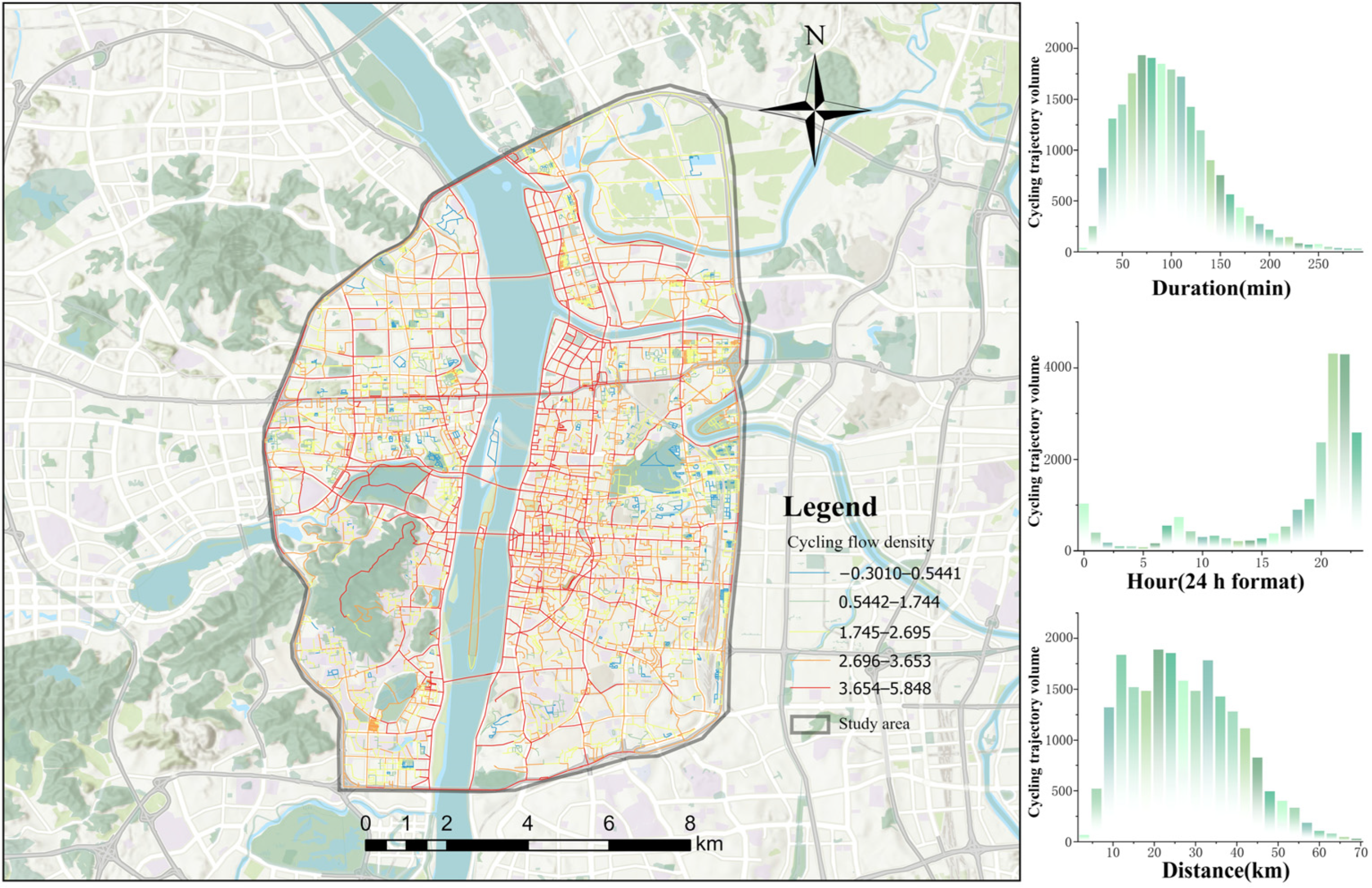
The study area is defined as the urban core street space enclosed by the Second Ring Road of Changsha, as shown in Figure 1. Located in the metropolitan core of Changsha, the capital of Hunan Province, the geographical center of the study area is approximately 28°13′41″ N, 112°56′20″ E. Climatically, Changsha features a humid subtropical climate characterized by an annual average temperature of approximately 17 °C, abundant precipitation, and distinct seasonal distribution, creating conditions favorable for year-round active outdoor activities such as walking, jogging, and cycling. The terrain is primarily composed of the Xiangjiang Plain, complemented by local mountainous landscapes such as Yuelu Mountain. With urban green spaces and riverfront corridors traversing from east to west, the area concentrates Changsha’s administrative, commercial, cultural, and transportation functions, providing critical physical venues and facility support for active outdoor leisure activities.

3.2. Data Collection and Preprocessing

3.2.1. Motion GPS Trajectories

GPS sports trajectories were recorded via fitness tracking applications, ensuring that the process did not involve personally identifiable information. The collected data primarily comprised User IDs, timestamps, and geographic coordinates (latitude and longitude). Utilizing the platform’s OAuth 2.0 protocol to obtain temporary access tokens, non-sensitive, publicly shared data—including exercise duration, timestamps, and anonymized trajectories—between March 2024 and March 2025, were harvested in this study with a sampling interval of 1–2 s. ArcGIS 10.5 was utilized to visualize and project the sampling points. After the removal of outliers and null values and application of the intersection tool to retain data within the study area, the final dataset yielded 50,840 trajectories (8809 walking, 20,177 jogging, and 21,854 cycling).

3.2.2. Streets and Roads

Street segments within the Second Ring Road of Changsha were selected as the spatial units of analysis, utilizing the following data extraction procedure: First, road network data for Changsha (dated March 2024) was downloaded via OpenStreetMap. Using ArcGIS 10.5, the data was clipped to the Second Ring Road of Changsha, and the network was simplified to extract road centerlines. Second, urban roads serving primarily transit functions—such as expressways, highways, and overpasses—were removed, while cross-river connections like the Juzizhou Bridge and Yingpan Road Tunnel were retained to accommodate cross-river traffic requirements. Finally, the retained roads underwent topological processing and were segmented at intersections to complete the network simplification, resulting in a total of 9083 street segments.

3.2.3. Street View Images

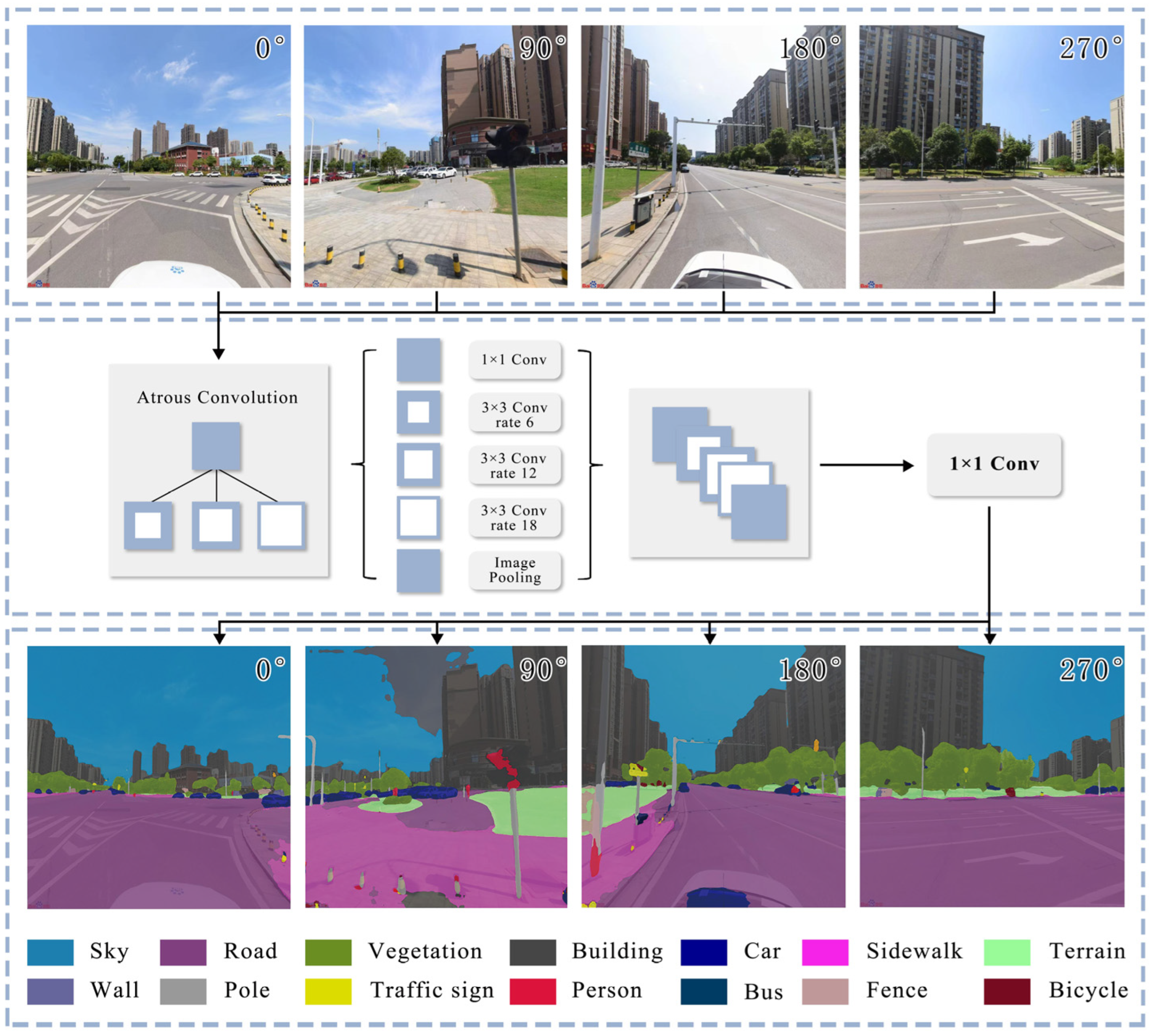
Based on the simplified road network data, coordinates for sampling points were generated at 50 m intervals. The Baidu Street View API was utilized to acquire Street View images for each sampling point based on geographic coordinates, with the vertical viewing angle set to 90° and horizontal viewing angles set to 0°, 90°, 180°, and 270° (Figure 2). The DeepLab V3+ model was employed for Street View sampling and semantic segmentation, and to address inconsistencies in image update times, the most recent image available for each location was selected. After the exclusion of sampling points with missing or incomplete images, the final dataset consisted of 18,794 sampling points and 75,176 Street View images. The Street View data covered 8751 streets, and supplementary field sampling was conducted for streets with missing data to ensure comprehensive coverage for every sampling point.

3.2.4. Other Datasets

To mitigate the interference of non-physical environmental variables, such as large-scale outdoor sports events and extreme weather, on population density data, heat map data from a continuous week characterized by fair weather and the absence of major events were selected as a representative proxy for population density.

3.3. Variables

3.3.1. Dependent Variables

Drawing on prior research [38], walking, jogging, and cycling flows were modeled as separate dependent variables in this study. The volume of outdoor activity for each street segment was derived using the following procedure: hierarchical buffers were established for roads of varying grades (

Table 1. Road grade and corresponding buffer zone distance.

Road Grade	Road Width (m)	Buffer Zone Distance (m)
Main road	45–55	55
Secondary road	40–50	50
Branch line	15–30	30

) to aggregate the trajectory points for walking, jogging, and cycling within each segment; these counts were then divided by the segment length to calculate the flow density for each activity type.

3.3.2. Independent Variables

Based on existing objective factors and the subjective factors extracted previously, built environment variables were selected across three dimensions: attractiveness, vitality, and accessibility (

Table 2. Built environment variables.

Category of Variable	Name of Variable	Abbr.	Description or Calculation	Unit
Accessibility	Bus stop density	D_BS	Number of bus stops/TAZ area size	points/m
	Road intersection density	D_RI	Number of intersections/TAZ area size	points/km
	Distance to nearest subway entrance	D_SBE	Distance from the nearest subway entrance to TAZ centroid	m
	Walking continuity	C_W		/
Vitality	Land use mix	LUM		/
	Population density	D_P	Population/TAZ area	persons/km2
	Retail store density	D_RS	Number of retail stores/TAZ area size	points/m
Attraction	Accessibility of large open spaces	ALOS	Distance to large open spaces (standardized)	/
	Sky openness	SO	SO = SO_x/i/n, (i = 1, …, n) The proportion of sky pixels in the i-th sampling point	/
	Green view index	GVI	$\mathrm{G}\mathrm{V}\mathrm{I}=\mathrm{G}\mathrm{V}{\mathrm{I}}_x/n,\left(i=1,\dots ,n\right)$ The proportion of vegetation pixels in the i-th sampling point	/
	Interface enclosure	IE	The ratio of building height to street width	/
	Building continuity	C_B		/

). Additionally, considering the spillover effects of road width and the built environment on movement flow [11], hierarchical buffers were established along road centerlines to quantify these variables. Previous studies [10] indicate that green and open spaces significantly attract physical activity. The green view index (GVI), sky openness (SO, accessibility of large open spaces (ALOS), interface enclosure (IE), and building continuity (C_B) were selected to measure the attractiveness of the built environment for outdoor street activities. Regional vitality factors, such as population density, land use mix, and commercial density, also significantly influence residents’ outdoor activities [7,33]. Drawing on existing research, population density (D_P), land use mix (LUM), and retail store density (D_RS) were chosen to characterize street vitality. Destination accessibility is a critical determinant of resident travel behavior [39]. Street accessibility was measured in this study using road intersection density (D_RI), bus stop density (D_BS), walking continuity (C_W), and distance to the nearest subway entrance (D_SBE).

3.4. Methods

3.4.1. Random Forest Model

The Random Forest ensemble machine learning algorithm [40] was employed in this study to effectively capture the potential nonlinear and high-dimensional complex relationships between the built environment and outdoor physical activity and to overcome the limitations of traditional linear models in addressing such issues. The core principle of Random Forest lies in the synergistic application of bootstrap aggregation and the random subspace method [40]. Specifically, the model first generates multiple sub-training sets from the original training set via bootstrap sampling, subsequently constructing an independent decision tree for each subset [41]. During the node splitting process for each tree, rather than selecting the optimal split from all built environment features, the model randomly selects a feature subset (typically the square root of the total number of features) and determines the optimal split point from within this subset [41]. The main formula is as follows:

$$H\left(x\right)=\underset{y}{\mathrm{a}\mathrm{r}\mathrm{g}\mathrm{m}\mathrm{a}\mathrm{x}}\sum _{i=1}^{n}I\left[h_i\left(x\right)=Y\right]$$

In the formula, $H\left(x\right)$ represents the output classification result; $h_i$ represents a single decision tree; $Y$ is the output variable; and $I$ is the feature function.

This dual randomness mechanism—comprising the random sampling of data and the random selection of splitting features—effectively reduces model variance, renders the model insensitive to data noise and outliers, and significantly enhances generalization capability, thereby overcoming the tendency of single decision trees to overfit.

In this study, the Random Forest model serves as a baseline and is compared in terms of performance with models such as Ordinary Least Squares (OLS) regression and Gradient-Boosted Decision Trees (GBDT) [42]. Its predictive accuracy was quantitatively evaluated using metrics such as Root Mean Square Error (RMSE) and Mean Absolute Error (MAE) [42]. More importantly, the complex data patterns identified using the Random Forest model establish a reliable predictive foundation for subsequent in-depth, interpretable mechanistic analysis using the SHAP framework. The aim of this study was to systematically reveal the driving mechanisms of the built environment on residents’ leisure physical activities from both “correlation” and “causality” perspectives by combining the high-precision prediction of Random Forest with the powerful interpretability of SHAP.

3.4.2. Interpretation Model

While the Random Forest model demonstrates superior predictive accuracy, its “black box” nature impedes a deep understanding of the mechanisms by which built environment factors influence outdoor physical activity [43]. To address this limitation and enhance model interpretability and transparency, this study introduces the SHAP framework—based on Shapley values from cooperative game theory—to decompose and elucidate model predictions at both global and local levels [43]. The core advantage of this framework lies in its ability to fairly attribute any given prediction value to individual input features, thereby achieving precise quantification of both single-variable contributions and their interaction effects. Specifically, the SHAP value of feature $i$ is determined according to its marginal contribution, calculated using the following formula:

$${\mathrm{\varnothing }}_i=\sum _{S\subset N\backslash \left\{i\right\}}{\displaystyle \frac{\left|S\right|!\left(\left|N\right|-\left|S\right|-1\right)!}{\left|N\right|!}}\left[f\left(S\cup \left\{i\right\}\right)-f\left(S\right)\right]$$

where N represents the set of all features, and $S$ is any subset of features excluding feature $i$. $f\left(S\right)$ represents the model prediction using feature subset $S$, while $f\left(S\cup \left\{i\right\}\right)$ represents the prediction after adding feature $i$. This formula ensures fairness and consistency in contribution allocation by calculating the weighted average of the marginal contributions of feature $i$ across all possible feature combinations. A feature’s SHAP value can be positive or negative, indicating a promotion or inhibition effect, respectively, on movement flow within that specific context. By calculating the mean of the absolute SHAP values for feature $i$ across all samples, the global importance metric (${\mathrm{\varnothing }}_i$) is obtained. This metric offers greater reliability than traditional importance metrics based on node impurity reduction:

$$\begin{array}{r}{I}_i={\displaystyle \frac{1}{n}}{\displaystyle \sum _{k=1}^n}\left|{\mathrm{⌀}}_i^{\left(k\right)}\right|\end{array}$$

Crucially, SHAP interaction values were further utilized in this study to capture and quantify bilateral interactions between built environment factors. The SHAP interaction value between feature $i$ and feature $j$(${\mathrm{⌀}}_{i,j}$) is defined by the following equation:

$${\mathrm{⌀}}_{i,j}=\sum _{S\subset N\backslash \{i,j\}}{\displaystyle \frac{\left|S\right|!\left(\left|N\right|-\left|S\right|-2\right)!}{2\left(\left|N\right|-1\right)!}}{\delta }_{i,j}\left(S\right)$$

In the formula,

$${\delta }_{i,j}\left(S\right)=f\left(S\cup \{i,j\}\right)-f\left(S\cup \left\{i\right\}\right)-f\left(S\cup \left\{j\right\}\right)+f\left(S\right)$$

${\delta }_{i,j}\left(S\right)$ quantifies the synergistic effect produced when features $i$ and $j$ coexist; a value greater than 0 indicates a positive interaction (synergy), while a value less than 0 indicates a negative interaction (offsetting effect). This enables the study to transcend the analysis of independent single-factor effects and deeply investigate how built environment elements couple to jointly influence residents’ physical activity decisions. For instance, does the synergistic effect of a high green view ratio and high functional density significantly promote walking flow? What type of interaction exists between high-quality cycling facilities and low motor vehicle interference?

In summary, through the application of the TreeExplainer within the SHAP package, the relative importance ranking of built environment factors was clearly defined, and the complex pathways influencing the spatial differentiation of urban street leisure activities from three dimensions of “global importance,” “local contribution direction,” and “inter-factor interaction mechanisms” were systematically revealed. This granular mechanistic analysis provides a solid scientific basis for formulating precise, empirically grounded strategies for healthy city and block design.

3.4.3. Research Framework

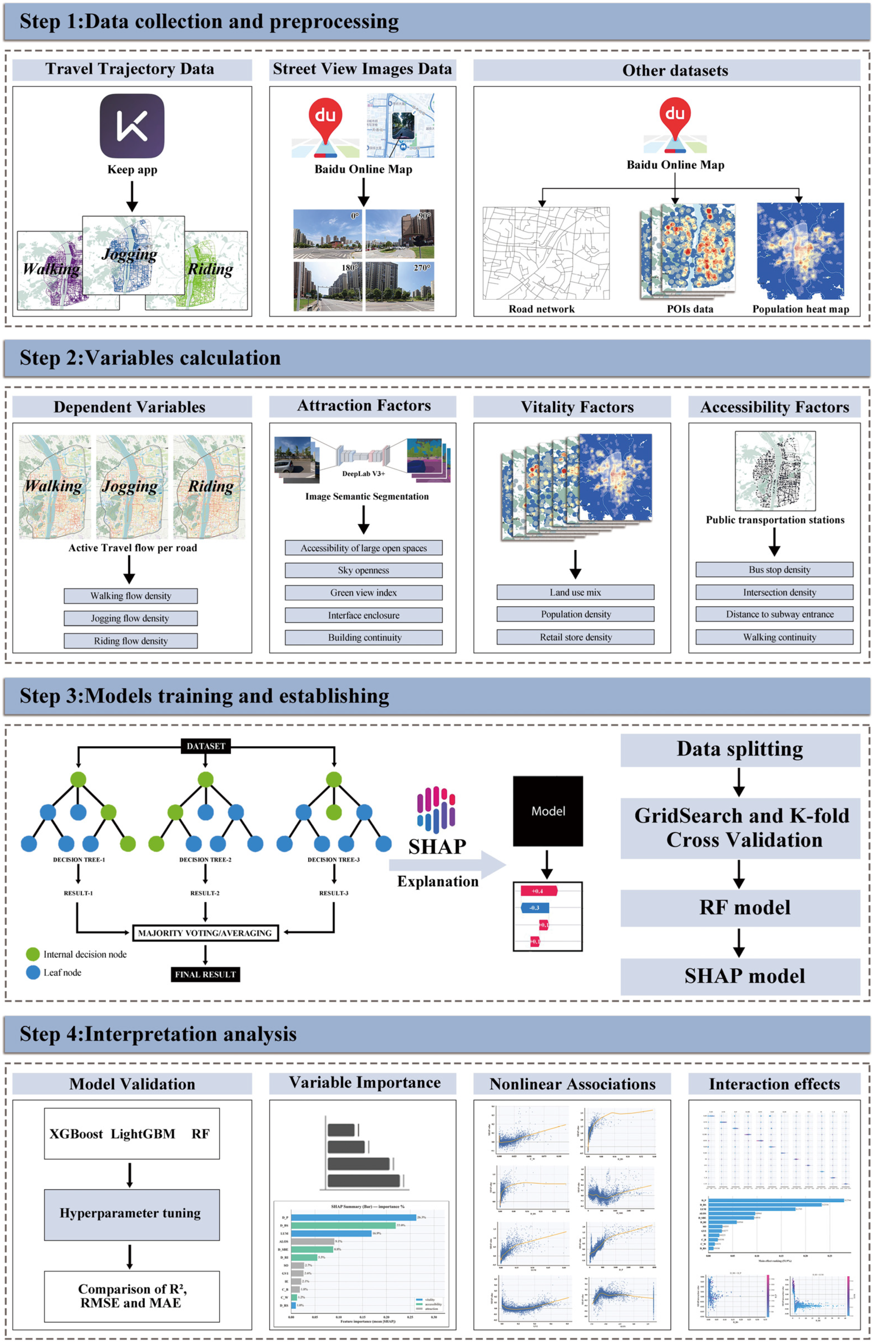
Figure 3 outlines the study’s four-step methodology: data collection and processing, variable calculation, Random Forest regression modeling, and global explanation using the SHAP method. In the data collection and processing phase, trajectory data for the three types of physical activities were aggregated with built environment predictors and spatially joined to the study units. The dependent variables were defined as cycling, jogging, and walking flows, while independent variables consisted of built environment features categorized into accessibility, vitality, and attractiveness characteristics. Following variable calculation, Random Forest, XGBoost 3.0.5, and LightGBM 4.6.0 regression models were compared within a Python 3.13.5 environment. The Random Forest model was ultimately selected for modeling, with 70% of the dataset used for training and 30% for testing to verify accuracy, utilizing GridSearchCV and K-Fold Cross Validation in Scikit-learn for hyperparameter tuning. Subsequently, the SHAP package was employed to calculate SHAP values, quantifying the impact of each built environment factor on physical activity flow to interpret model predictions. Finally, SHAP interaction values were calculated to explore the interaction effects between different built environment factors.

4. Results

4.1. Descriptive Analysis

4.1.1. Walking GPS Trajectories

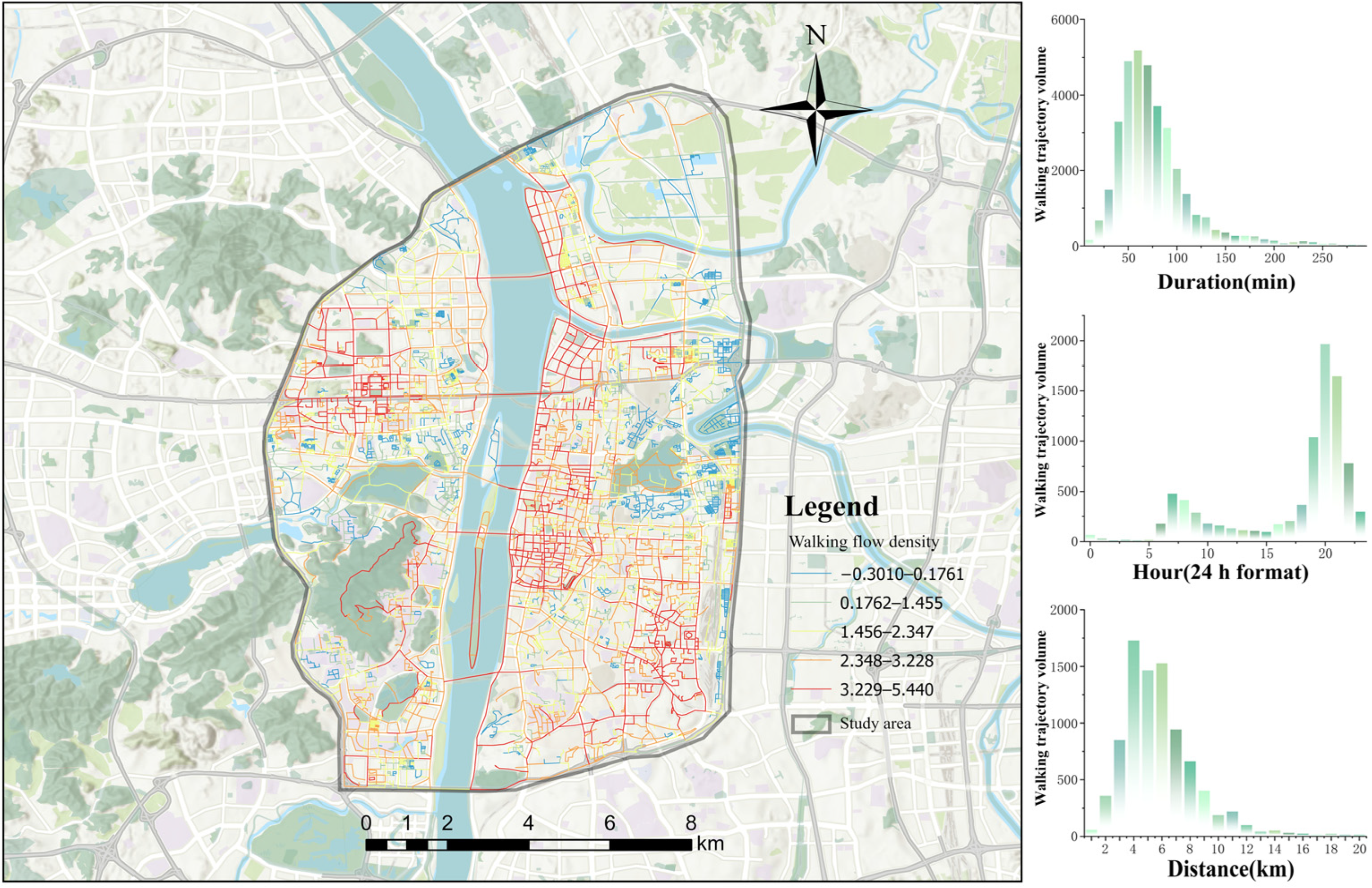
In terms of trajectory distance (Figure 4), outdoor walking in Changsha is predominantly medium-distance; trajectories of 2–4 km account for approximately 29% of the total, while those of 4–6 km and 6–8 km constitute 33% and 18%, respectively, demonstrating a reduction in quantity with increasing distance that aligns with the geographical law of distance decay. Regarding duration (Figure 4), the average outdoor walking time is 78 min, with trajectories lasting 60–120 min comprising approximately 83.92% of the total; walking flow significantly decreases as duration extends beyond this range. In terms of temporal distribution (Figure 4), walking activity volume exhibits distinct variations across different times of the day. Walking activity displays morning and evening peaks (07:00–09:00 and 19:00–21:00) with peak values at 07:00 and 20:00, indicating that Changsha residents primarily engage in exercise during these times to avoid commuting rush hours. Spatially (Figure 4), outdoor walking is characterized by distinct aggregation, forming a multi-center radial pattern anchored by Wuyi Square, Beichen Delta, Bafang Park, and Dongtang. Notably, walking flow from Wuyi Square spills over northward along the Xiang River, merging with the outflow from Beichen Delta to form a high-density walking belt along the Xiang River Scenic Belt. High population density around Wuyi Square and Dongtang provides the demographic base for outdoor activities, while the comprehensive sports and leisure infrastructure in riverside areas and parks, combined with superior blue–green spaces, attracts further flow and offers suitable venues for outdoor exercise.

4.1.2. Jogging GPS Trajectories

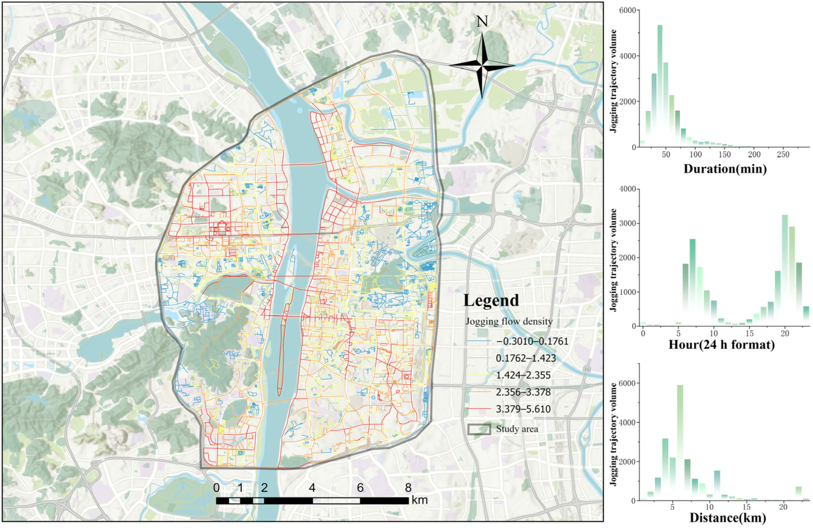
Summarizing the jogging trajectories (Figure 5), residents’ outdoor jogging is primarily medium-distance; trajectories of 2–4 km account for approximately 22% of the total. Trajectories of 4–6 km and 6–8 km account for 40% and 16% of the total, respectively. Notably, jogging flow increases significantly at a distance of 11 km, which approximates a quarter marathon, suggesting the influence of sports event training. Regarding duration (Figure 5), the average outdoor run time is 35 min, with trajectories under 60 min comprising approximately 81.36% of the total. Similarly to walking, jogging flow shows a significant downward trend as duration increases. In terms of temporal distribution (Figure 5), jogging activity also exhibits morning and evening peaks (06:00–09:00 and 19:00–22:00), with peak values at 07:00 and 20:00. Jogging peaks last longer and feature higher volume during the morning peak than those of walking, indicating a stronger preference for morning exercise among runners. Spatially (Figure 5), outdoor jogging displays distinct aggregation, forming high-density core areas centered on Bafang Park, Beichen Delta, and Dongtang, with flow decreasing from these cores to the periphery. It is worth noting that linear high-density core areas form along both banks of the Xiang River, Wuyi Avenue, and Furong Middle Road, aligning closely with Changsha’s blue–green corridors.

4.1.3. Cycling GPS Trajectories

Cycling trajectory data (Figure 6) reveals that residents’ outdoor cycling is predominantly long-distance, exhibiting an atypical decay distribution. Distances of 10–20 km, 20–30 km, and 30–40 km account for 25%, 26%, and 22%, respectively, constituting the core cluster. The average outdoor cycling duration is 97 min, with the distribution showing a right-skew; the 60–120 min range forms the core distribution band, accounting for 49% of total trajectories. Cycling activity also shows morning and evening peaks (08:00–10:00 and 19:00–22:00), peaking at 09:00 and 21:00. The partial overlap between the morning peak and commuting rush hours further reflects the short-distance connecting function of outdoor cycling. Some cycling enthusiasts exhibit unconventional activity patterns, such as a small amount of cycling occurring between 24:00 and 02:00. Cycling shows less distinct spatial aggregation (Figure 6) than walking and jogging, with higher flow around Beichen Delta, Xianjia Lake–Yuelu Mountain, and Wuyi Square. Cycling flow decreases along the street hierarchy, suggesting that the built environment of lower-level streets fails to meet cycling needs, forcing activity toward higher-level streets. The use of bicycles overcomes human physical limits, extending the single-activity radius to four times that of walking or jogging, reducing spatial aggregation, and ultimately forming a weakly centralized distribution pattern characterized by “corridor dominance and region-wide permeation.”

4.2. Model Training and Evaluation

The Variance Inflation Factor (VIF) was employed in this study to test for multicollinearity among built environment variables. As shown in

Table 3. Variance inflation factors. Variables in the table represent: D_RS, retail store density; ALOS, accessibility of large open spaces; LUM, land use mix; D_RI, road intersection density; D_BS, bus stop density; D_SBE, distance to nearest subway entrance; D_P, population density; C_W, walking continuity; C_B, building continuity; GVI, green view index; SO, sky openness; IE, interface enclosure.

Variable	VIF	Tolerance
D_RS	1.065	0.939
ALOS	1.079	0.926
LUM	1.154	0.866
D_RI	1.194	0.838
D_BS	1.287	0.777
D_SBE	1.323	0.756
D_P	1.368	0.731
C_W	1.538	0.650
C_B	1.543	0.648
GVI	2.016	0.496
SO	2.270	0.440
IE	2.489	0.402

, all VIF values are less than 5, indicating no serious multicollinearity; thus, all variables were retained [44]. During model training, bootstrap sampling was used; 80% of the original sample served as training data and the remaining 20% as testing data to evaluate Random Forest (RF) model performance, while grid search and 5-fold cross-validation were employed to determine optimal parameter combinations and prevent overfitting. Based on existing research [45], three parameters—maximum tree depth, minimum samples required for node splitting, and the number of trees in the forest—are critical for enhancing Random Forest model performance. Therefore, the widely used grid search method was adopted to identify optimal parameters within the selected range. The optimal parameters for the RF model were set as follows: 500 iterations and a maximum tree depth of 13. Finally, Root Mean Square Error (RMSE), Mean Absolute Error (MAE), and R² were used as evaluation metrics to compare the performance of the RF model with XGBoost and LightGBM models [46]. The results from

Table 4. Cycling traffic model parameters and evaluation.

Model	Parameters			Performance
	N_Estimators	Learning Rate	Max_Depth	RMSE	MAE	R2
RF	500	/	13	0.892	0.680	0.682
XGBoost	100	0.14	6	0.929	0.695	0.655
LightGBM	400	0.04	15	0.940	0.716	0.646

,

Table 5. Jogging traffic model parameters and evaluation.

Model	Parameters			Performance
	N_Estimators	Learning Rate	Max_Depth	RMSE	MAE	R2
RF	500	/	13	0.719	0.519	0.660
XGBoost	100	0.14	6	0.750	0.524	0.631
LightGBM	400	0.04	13	0.762	0.545	0.619

and

Table 6. Walking traffic model parameters and evaluation.

Model	Parameters			Performance
	N_Estimators	Learning Rate	Max_Depth	RMSE	MAE	R2
RF	500	/	13	0.746	0.551	0.662
XGBoost	100	0.15	6	0.774	0.560	0.637
LightGBM	400	0.04	19	0.797	0.590	0.615

indicate that the RF model possesses higher goodness-of-fit and outperforms the other two machine learning models.

4.3. BE Variable Importance

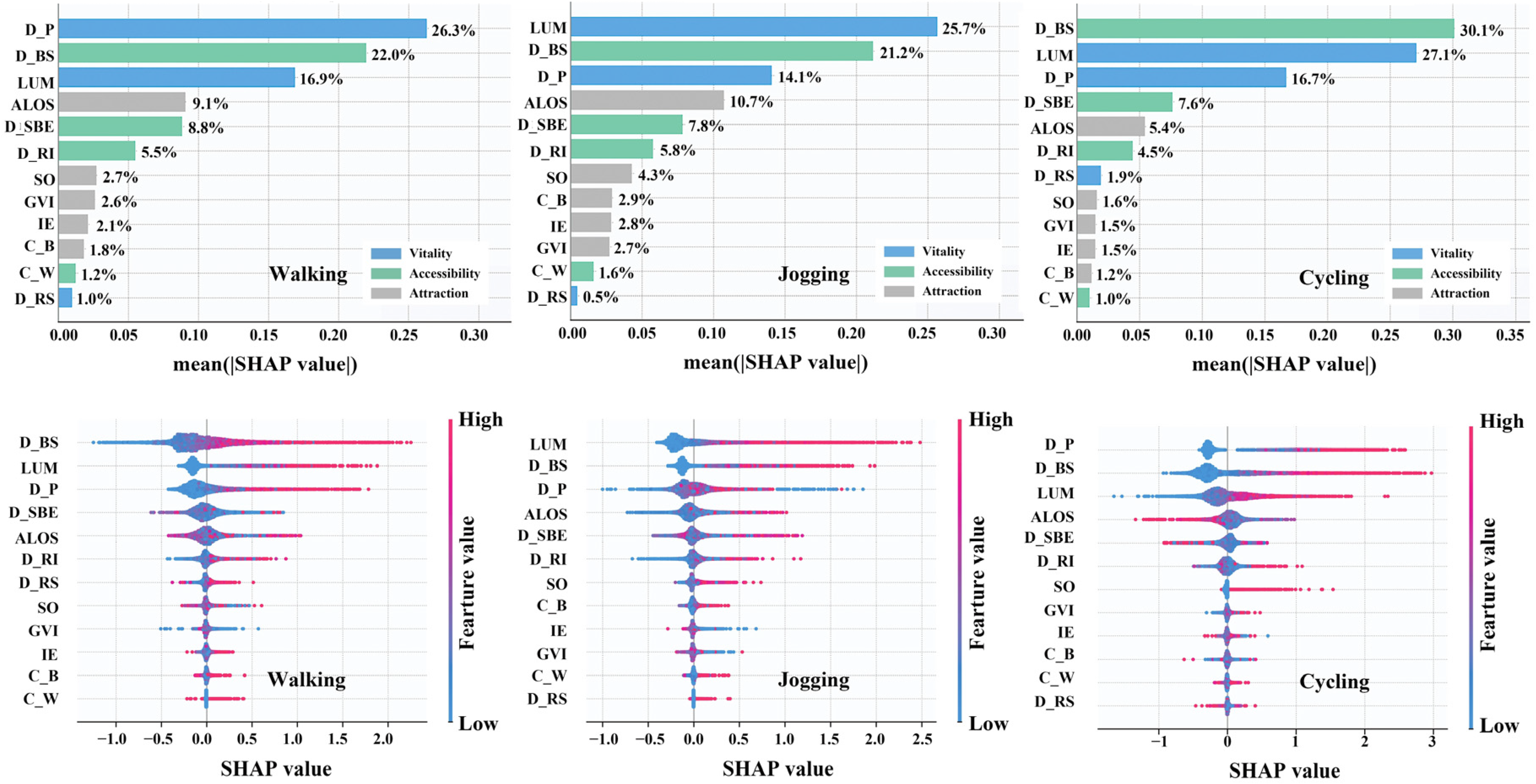
The global contributions of the twelve built environment variables were calculated using mean SHAP values (Figure 7).

Table 7. Contribution of built environment. Variables in the table represent: D_BS, bus stop density; LUM, land use mix; D_P, population density; D_SBE, distance to nearest subway entrance; ALOS, accessibility of large open spaces; D_RI, road intersection density; D_RS, retail store density; SO, sky openness.

Activity	Category of Variable	Name of Variable	Contribution
Cycling	Accessibility	D_BS	30.1%
	Vitality	LUM	27.1%
	Vitality	D_P	16.7%
	Accessibility	D_SBE	7.6%
	Attraction	ALOS	5.4%
	Accessibility	D_RI	4.5%
	Vitality	D_RS	1.9%
	SUM		93.3%
Jogging	Vitality	LUM	25.7%
	Accessibility	D_BS	21.2%
	Vitality	D_P	14.1%
	Attraction	ALOS	10.7%
	Accessibility	D_SBE	7.8%
	Accessibility	D_RI	5.8%
	Attraction	SO	4.3%
	SUM		89.6%
Walking	Vitality	D_P	26.3%
	Accessibility	D_BS	22.0%
	Vitality	LUM	16.9%
	Attraction	ALOS	9.1%
	Accessibility	D_SBE	8.8%
	Accessibility	D_RI	5.5%
	Attraction	SO	2.7%
	SUM		91.3%

clearly illustrates the top seven contributing variables for each activity type along with the magnitude of their contributions.

It is evident that vitality and accessibility variables dominate in walking, jogging, and cycling activities, accounting for approximately 90% of the variance in the three physical activity models, whereas attractiveness variables explain only about 10%. This suggests that transportation accessibility and the density represented by vitality are closely correlated with physical activity, while streetscape attributes may not be significantly associated factors.

4.4. Nonlinear Associations of BE Variables

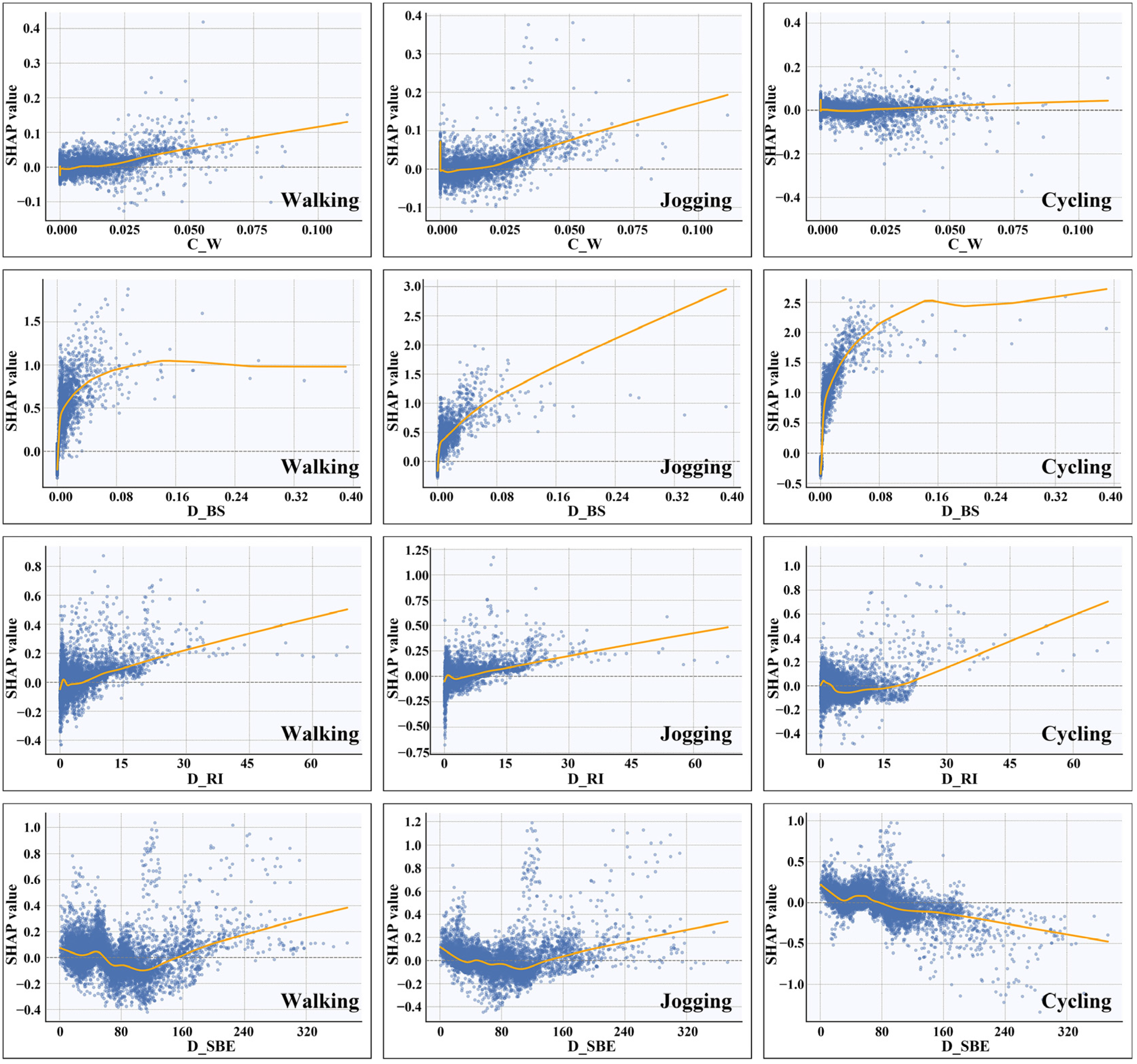
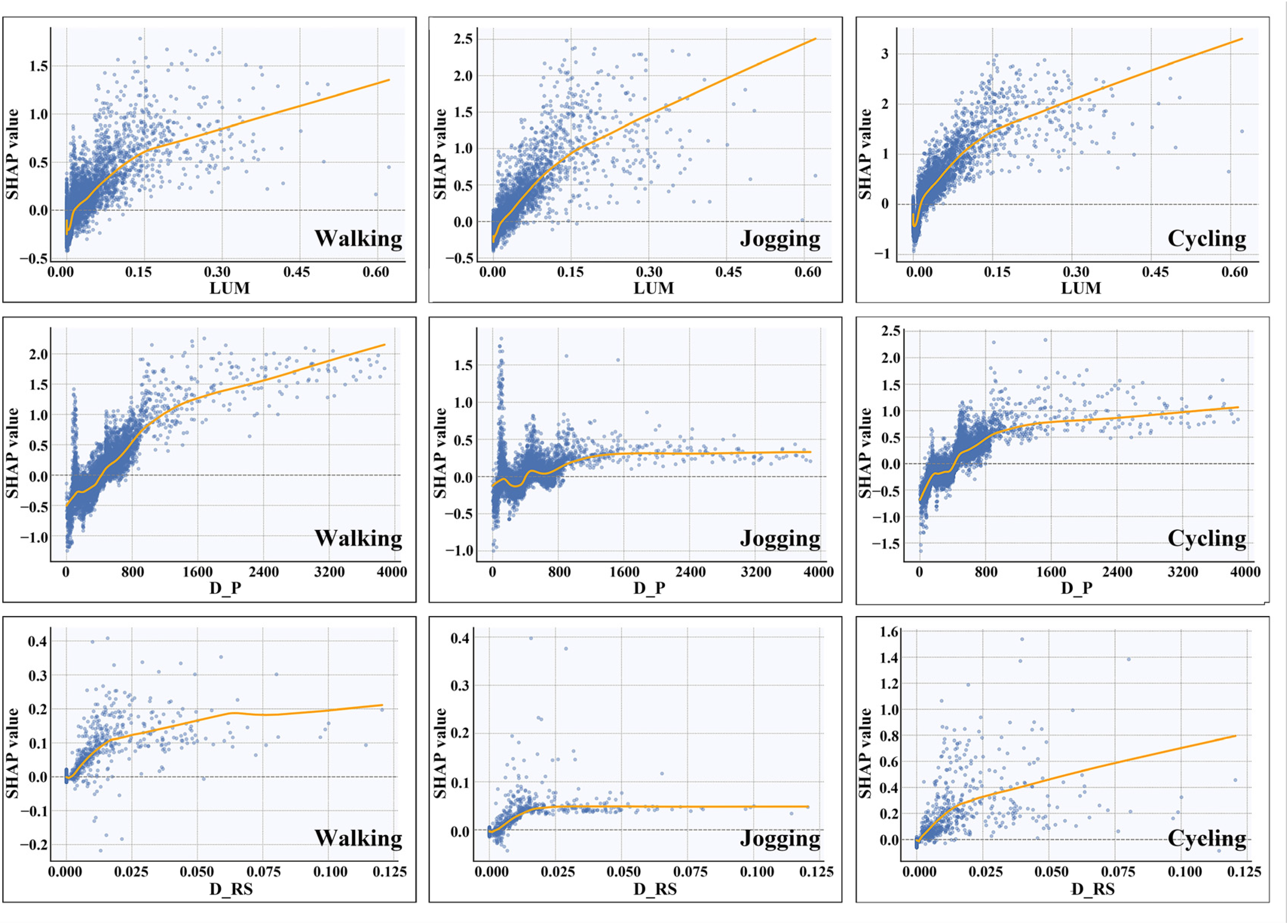
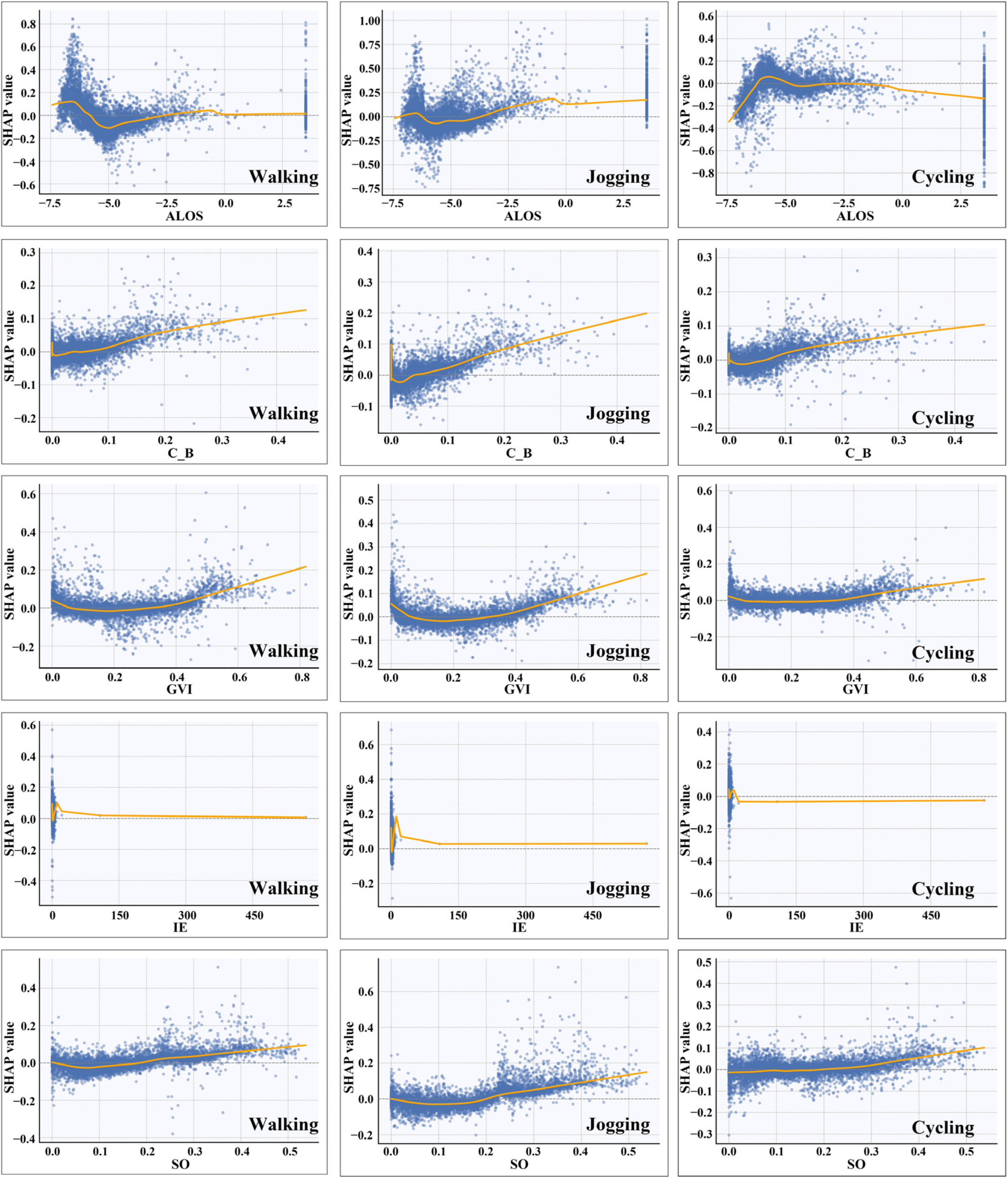
SHAP-based Local Dependence Plots (LDPs) were employed to reveal the nonlinear effects of built environment variables across the dimensions of accessibility, vitality, and attractiveness on walking, jogging, and cycling flows (Figure 8, Figure 9 and Figure 10).

4.4.1. The Variables of Accessibility

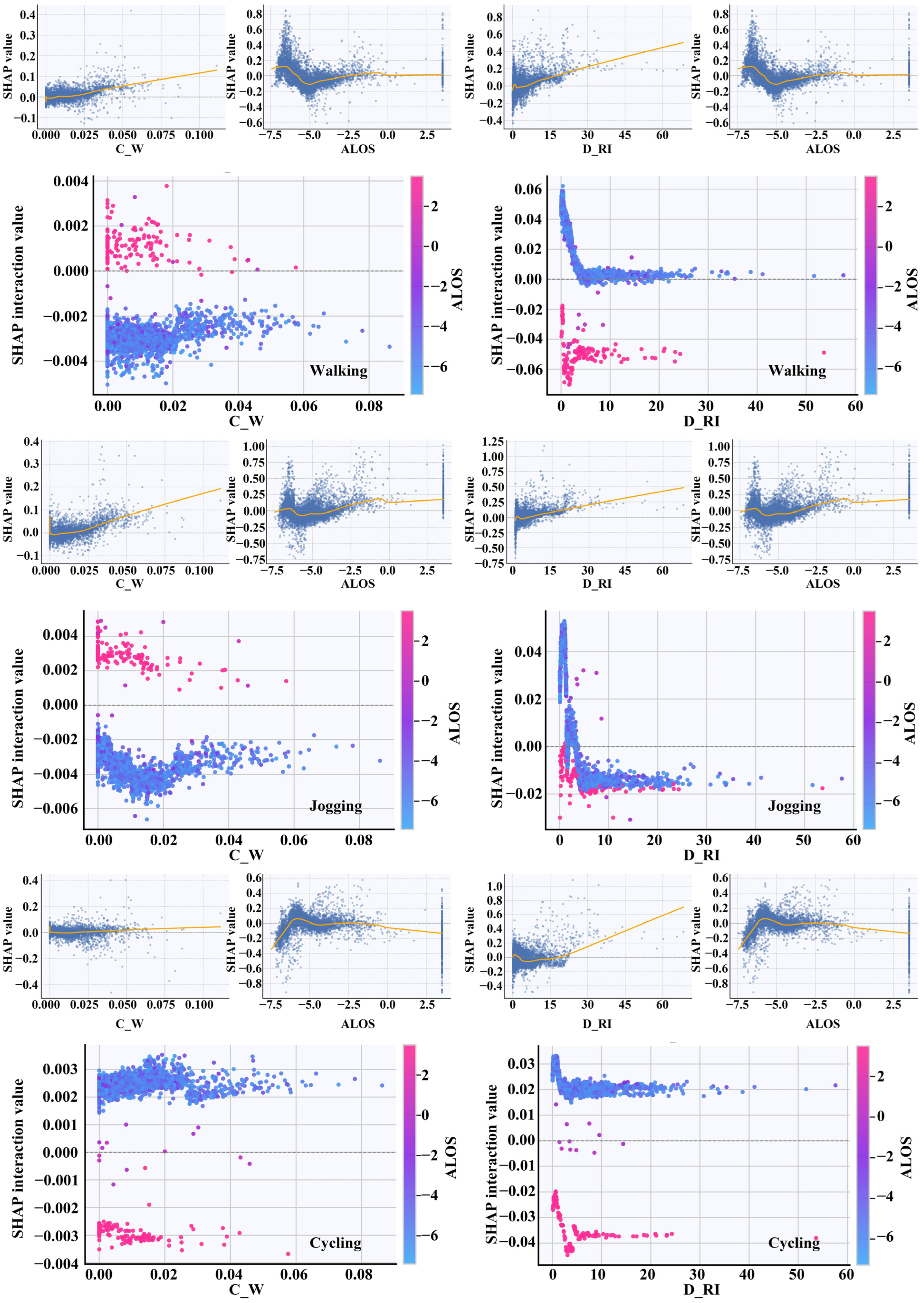
Figure 8 illustrates the nonlinear effects of accessibility built environment (BE) variables on walking, jogging, and cycling. C_W exerts a positive influence on walking, jogging, and cycling flows. When C_W exceeds 0.007, the local effects for jogging and walking shift from negative to positive. When this variable exceeds 0.025, the local effect for cycling also transitions from negative to positive. Subsequently, as the variable increases, the rate of change in local effects descends in the order of jogging, walking, and cycling. This indicates that increased sidewalk width provides greater space for physical activities, with jogging being the most sensitive to this change. D_BS also positively impacts all three types of physical activities. When D_BS exceeds 0.001 stations/m, the local effects for all three activities shift from negative to positive, maintaining growth with a continuously decreasing slope. The slope of the local effect for jogging ceases to decrease once the variable exceeds 0.003 stations/m, maintaining a constant growth rate. When the variable exceeds 0.14 stations/m, the local effects for cycling and walking remain essentially unchanged, suggesting that the effective threshold for this variable has been surpassed. Previous studies explain that while public transport can promote physical activity [47], excessive transit density leads to overwhelming vehicular and pedestrian flows, causing psychological pressure on exercisers [48]. D_RI exerts a positive influence on the three physical activities. When D_RI exceeds 6 intersections/km, the local effects for jogging and walking transition from negative to positive. When this variable exceeds 18 intersections/km, the local effect for cycling also shifts from negative to positive. Thereafter, the local effect for cycling grows the fastest as the variable increases, while the changes for jogging and walking are identical. This implies that moderate street connectivity offers convenient pathways for physical activity [49] and that the supportive environments required differ among physical activities. D_SBE positively influences jogging and walking activities but negatively affects cycling. When D_SBE is between 300 m and 1400 m, the local effects for jogging and walking are negative; outside this range, they are positive. After the variable exceeds 800 m, the local effect for cycling shifts from positive to negative. As found in prior studies, convenient transportation attracts people engaging in physical activity for transfer purposes [50]; however, moving beyond the catchment area of the subway station diminishes this attraction [51].

4.4.2. The Variables of Vitality

Figure 9 illustrates the nonlinear effects of vitality BE variables on walking, jogging, and cycling. LUM has a positive impact on cycling, jogging, and walking flows. When LUM exceeds 0.01, the local effects for all three activities transition from negative to positive. This finding aligns with previous research [52], likely because increased LUM extends the duration of moderate-intensity physical activity [53]. Beyond the 0.01 threshold, as the variable increases, the growth rate of local effects descends in the order of cycling, jogging, and walking. D_P also exerts a positive influence on the three physical activities. After D_P exceeds 400 people/km², the local effects for all three activities shift from negative to positive. Subsequently, as D_P increases, the growth rate of local effects follows the order of walking, cycling, and jogging. A possible reason is that destinations in higher-density areas are closer, as the critical mass required to support physical activities can be found within smaller areas, though the correlation between D_P and different activities is not necessarily consistent [54]. D_RS positively impacts all three types of physical activity. As this variable increases, the growth rates of local effects descend in the order of cycling, walking, and jogging, which is consistent with previous findings [55].

4.4.3. The Variables of Attraction

Figure 10 illustrates the nonlinear effects of attractiveness BE variables on walking, jogging, and cycling. GVI exerts a positive influence on walking, jogging, and cycling flows. After the GVI exceeds 0.35, the local effects for all three activities transition from negative to positive. As the GVI increases further, the growth rates of local effects descend in the order of walking, jogging, and cycling. This may be because cycling is less sensitive to greenery on roads below the secondary highway level than other physical activities [56]. Furthermore, the changes in walking and jogging are essentially identical, which mirrors previous research results [57]. SO also positively influences the three physical activities. When the SO reaches 0.2, the local effects for all three activities shift from negative to positive. A likely reason is that a higher SO provides an open field of vision and sufficient sunlight [58]. Beyond 0.2, as the SO increases, the growth of local effects for the three activities is fundamentally consistent. ALOS negatively affects cycling and positively affects jogging; for walking, the effect is positive below −5.8, negative between −5.8 and −2.5, and negligible thereafter. This can be explained by prior research suggesting that a high proportion of open space near residences negatively impacts physical activity for commuting purposes [59], thus reducing attractiveness for cycling. Conversely, since the distance for recreational walking to open spaces is often short [60], this variable also exerts a partial positive influence on walking activity. As IE increases, its influence on the three activities shifts from positive to negative and then from negative back to positive. Ultimately, the negative local effect for cycling and the positive local effects for jogging and walking tend to stabilize. C_B exerts a positive influence on the three physical activities. When C_B exceeds 0.05, the local effects for walking and jogging transition from negative to positive. When this variable exceeds 0.07, the local effect for cycling also shifts from negative to positive. Thereafter, as the variable increases, the growth rate of local effects descends in the order of jogging, walking, and cycling.

4.5. Interaction Effects Among BE Variables

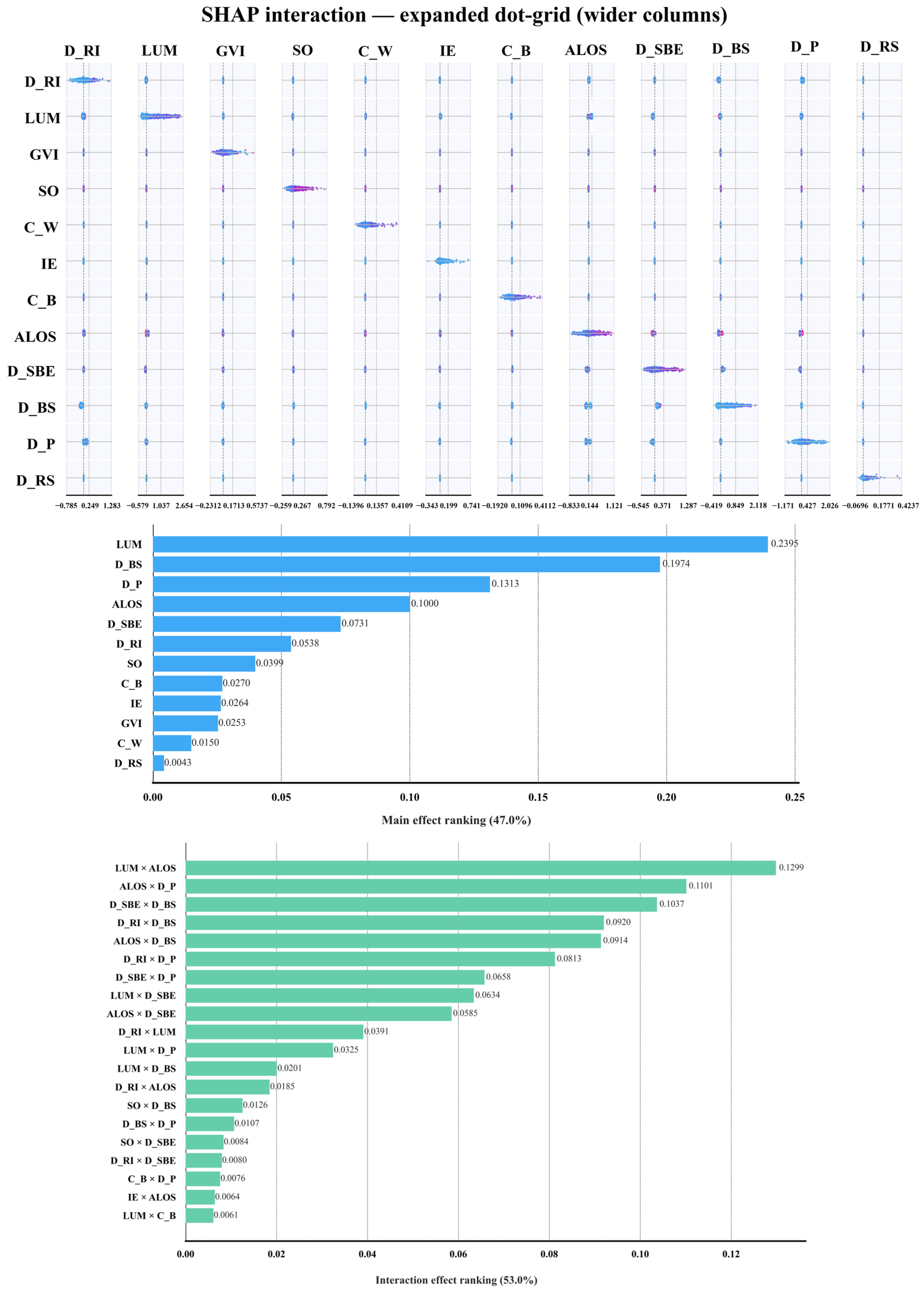
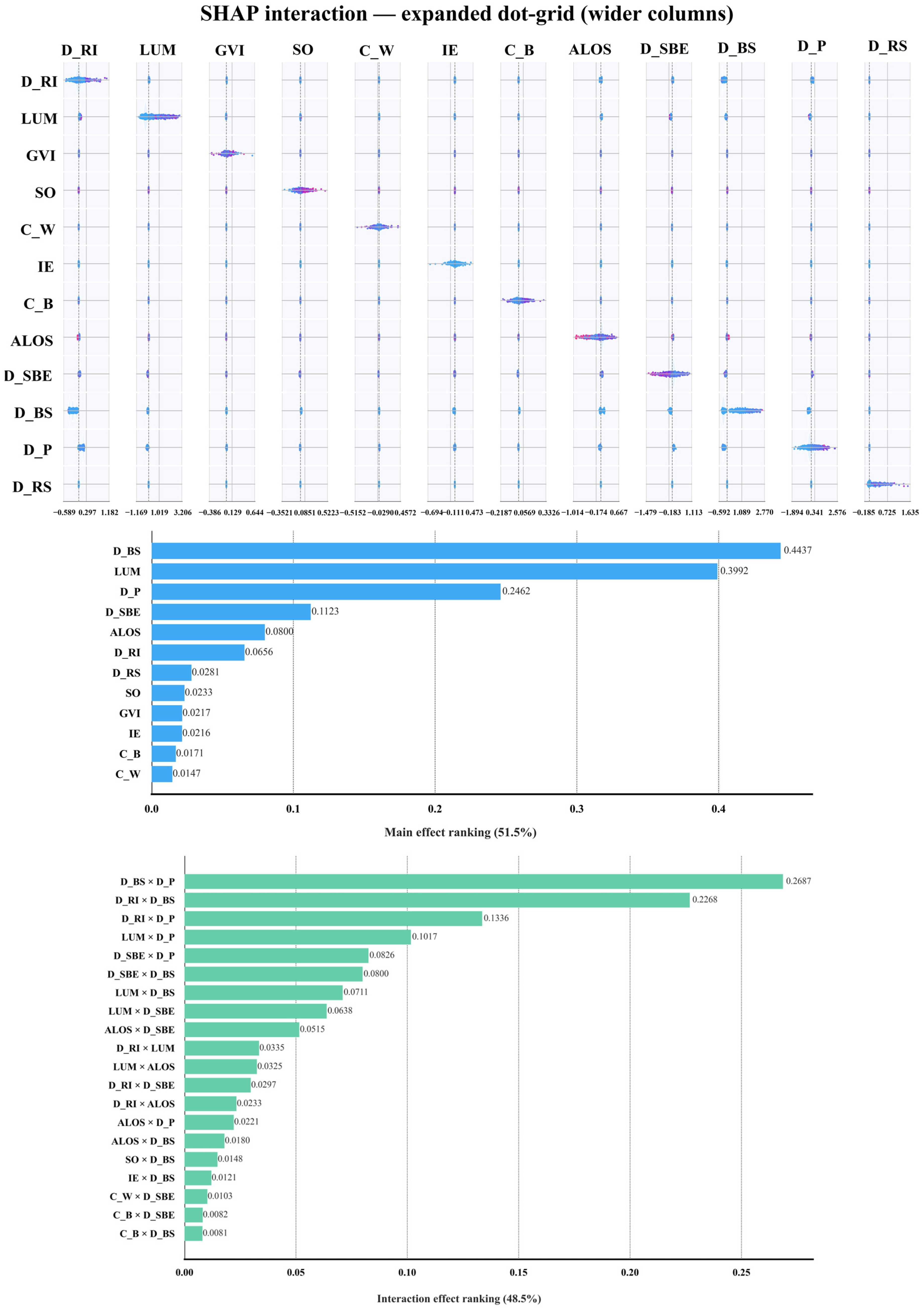
Using the Python SHAP library, the local effects (SHAP values) of the explanatory variables were decomposed into their main local effects (SHAP main effect values) and their local interaction effects with other variables (SHAP interaction values). The interaction effects of multi-level built environment variables on walking, jogging, and cycling flows were explored in this study (Figure 11, Figure 12 and Figure 13). Each graph corresponds to a pair of variables, and each point within the graph represents a specific observation. The color axis on the right indicates the value of the second variable in the pair, with deeper red representing higher values. A SHAP interaction value of 0 indicates no interaction; a value greater than 0 indicates a positive interaction effect; and a value less than 0 indicates a negative interaction effect.

4.5.1. Overall Analysis

By calculating the SHAP interaction values shown in the figures above, the main and interaction effects of all built environment factors were visualized. Generally, main effects exceed interaction effects. This holds true for cycling and walking flows, where the sum of main effects is higher than that of interaction effects. However, it is notable that some interaction effects surpass main effect values; for instance, in walking flow, the interaction effects of ALOS with both D_SBE and D_P exceed the main effect of ALOS, while the interaction between D_SBE and ALOS exceeds the main effect of D_SBE. Notably, the sum of main effects for jogging flow is lower than that of the interaction effects, indicating that interactions between variables are more critical for jogging activities. Additionally, interactions involving certain variables, such as GVI, are not prominent in the cycling and jogging flow interaction graphs because their SHAP interaction values are relatively low compared to the top-ranked variable pairs. This suggests that GVI influences these activities primarily through its main effects rather than through strong synergistic interactions with other built environment factors.

4.5.2. Interaction Analysis

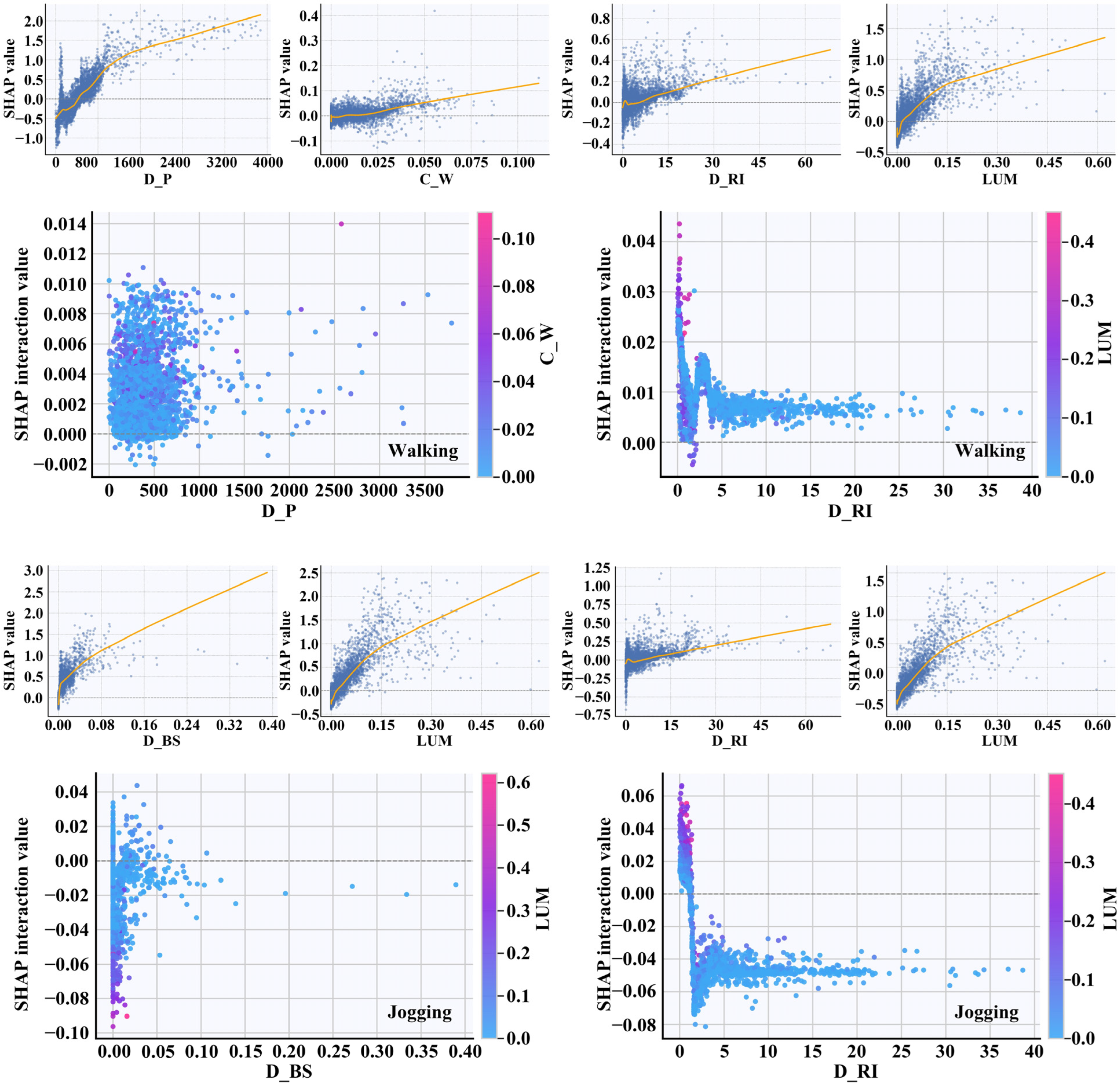
Specific interaction effects on the three activity types for accessibility–vitality (Figure 14), vitality–attractiveness (Figure 15), and attractiveness–accessibility (Figure 16) variable pairs. Several notable built environment variable pairs were selected for analysis.

(1)

Accessibility–vitality variable pairs

The results in Figure 14 show that for walking flow, D_P and C_W produce a positive interaction effect, which is consistent with their main effects. However, when D_P is between 0 and 1000 people/km² and C_W does not exceed 0.02, a negative interaction effect exists. This suggests that in low-density areas, walking can be promoted by increasing the proportion of sidewalks, aligning with prior research [61]. D_RI and LUM generate a positive interaction effect, consistent with their main effects. However, when D_RI is between 1 and 3 intersections/km and LUM is between 0.1 and 0.2, a negative interaction effect occurs. This indicates that in areas with sparse road networks, walking can be encouraged by diversifying land use types, which echoes previous findings [62]. Regarding jogging flow, D_BS and LUM produce a negative interaction effect, contrary to their main effects. When D_BS is between 0.00 and 0.05 stations/m, increasing station density can mitigate or reverse the negative interaction, whereas increasing LUM exacerbates it. This implies that in areas with low transit coverage, excessive LUM should be avoided to prevent inhibiting jogging. D_RI and LUM produce a negative interaction effect, contrary to their main effects. When D_RI exceeds 2 intersections/km, the interaction effect with LUM shifts from positive to negative. Increasing D_RI shifts the interaction effect toward the negative, whereas increasing LUM shifts it toward the positive. This suggests that in areas with high D_RI, diversifying land use types can mitigate the negative impact of pedestrian and vehicular flows on jogging, aligning with earlier studies [63].

(2)

Vitality–attractiveness variable pairs

In Figure 15, when ALOS exceeds 0, it interacts negatively with LUM (0.0–0.2 range) for walking and jogging flows as well as with D_P (0–1000 people/km² range) for walking flow but positively for jogging flow. This indicates that in low-D_P areas, excessive LUM should be avoided to prevent interference with walking and jogging activities. Furthermore, when D_P is low, large open spaces attract joggers but may hinder walking. Regarding cycling flow, when C_B exceeds 0.2, it produces a positive interaction with LUM (0.0–0.1 range), suggesting that in areas with single land use, cycling can be promoted by enhancing street façade integrity. When the SO is less than 0.2, it produces a negative interaction with LUM (0.00–0.05 range), indicating that areas with single land use can also promote cycling by enhancing the SO.

(3)

Attractiveness–accessibility variable pairs

According to Figure 16, when ALOS exceeds 0, it interacts positively with C_W for walking and jogging flows but negatively for cycling flow. This implies that the combination of large open spaces and sidewalks facilitates walking and jogging but inhibits cycling. Within the same value range, ALOS produces a negative interaction effect with D_RI (0–25 intersections/km range) for walking and cycling. Conversely, when D_RI does not exceed 4 intersections/km and ALOS does not exceed −2, these two variables exert a positive interaction effect on jogging flow. This suggests that in areas with sparse road networks, reducing ALOS is necessary to avoid interfering with physical activities such as walking, jogging, and cycling.

5. Discussion

5.1. Comprehensive Interpretation of BE Affecting Outdoor Activities

5.1.1. Influence of BE on Walking Behaviors

The results show that D_P (RI: 26.3%) and D_BS (RI: 22.0%) are the two most important predictors of residents’ walking behavior, which is highly consistent with [47]. This suggests that in high-density cities such as Changsha, walking is largely a purpose-driven activity closely linked to residents’ daily commutes, short transfers, and access to everyday services. Population concentration typically coincides with high-density provision of commercial and public services, which reduces travel distances, increases the feasibility of walking, and makes walking the primary mode for short trips [64]. At the same time, higher D_BS substantially improves accessibility and creates a walk–transit coupling effect that concentrates transfer, boarding/alighting, and waiting flows around stops, thereby forming local pedestrian catchment areas. SHAP partial dependence plots also provide key nonlinear evidence. When street population density exceeds the threshold of 400 people per square kilometer, it begins to exert a significant positive effect on walking flows, and the slope of the impact curve is the steepest among the three activity types. This result confirms that high D_P not only supplies a sufficient demand base—or “potential user pool”—for walking trips but also brings more destinations within residents’ walking reach, thereby enhancing convenience and making walking a more attractive travel mode. This is consistent with multiple studies reporting a nonlinear amplifying effect of D_P on walking [63]. A more critical insight comes from D_BS. Walking flows increase steadily with D_BS but begin to decline after density reaches approximately 0.14 stops/m and then level off after about 0.26 stops/m. This “saturation effect” is not captured by traditional linear models, whereas machine learning methods have recently been shown to identify such thresholds effectively in built environment–travel-behavior studies [65]. This finding aligns with the consensus in Wu et al. [63], who studied older adults and argued for an “effective range” of built environment attributes—i.e., the positive effects of high-density environments are not unbounded [63]. Research on pedestrian streets likewise finds that D_BS is an important promoter of walking activity but that clear nonlinear thresholds exist, which is highly consistent with our conclusions [64].

5.1.2. Influence of BE on Jogging Behaviors

Unlike the strong purposiveness of walking, jogging—as a typical leisure activity—exhibits a pronounced “experience-oriented” driving mechanism [66]. The results show that the three most important predictors of residents jogging behavior are LUM (RI = 25.7%), D_BS (RI = 21.2%), and ALOS (RI = 10.7%). The most significant finding regarding residents’ jogging behavior arises from the aggregate analysis of interaction effects among environmental variables. Interactions among built environment variables indicate that joggers typically seek a coherent street-environment experience rather than a single optimal setting (such as an isolated park); they value combinations of environmental elements, and the quality of an individual factor alone cannot fully determine a street’s attractiveness for jogging—the key is whether it combines with other factors to deliver a good experience for joggers [66]. SHAP interaction-effect analysis provides a concrete explanation for this pattern. When streets are proximate to large open spaces (ALOS < 0), higher LUM exerts a significant positive effect on jogging behavior, indicating that joggers prefer high-quality jogging environments that are also supported by convenient commercial services such as sports supply points, quick meals, or cafés. Conversely, when also close to open spaces (ALOS < 0), excessively high D_P produces a strong negative effect on jogging flows. This key finding suggests that joggers want proximity to park entrances but also desire to avoid the crowding and disturbances associated with high-density populations—they require scenic yet relatively quiet jogging environments [66]. Existing studies have highlighted the importance of parks and green open spaces for jogging [67,68], but our study further shows that these built environment elements must operate in specific combinations to be effective in attracting joggers. This also explains why some streets adjacent to parks have few joggers in practice: overly high D_P or insufficient LUM may generate negative interaction effects.

5.1.3. Influence of BE on Cycling Behaviors

Residents’ outdoor cycling serves both the “last-mile” function for commuting transfers and long-distance recreational purposes, and overall exhibits a clear efficiency orientation [69]. It was found in this study that cycling flows are primarily driven by D_BS (RI = 30.1%) and LUM (RI = 27.1%), and SHAP analysis further elucidates the underlying mechanisms. First, cycling is most sensitive to LUM, exhibiting the steepest slope on the response curve. Higher LUM typically indicates close co-location of commercial, leisure, and office uses. Such agglomeration substantially shortens trip distances and increases available destination choices, thereby promoting cycling for both commuting and recreational purposes [70]. The efficiency demand of cycling is also reflected in accessibility indicators [71]. When the distance to a metro entrance exceeds approximately 800 m, cycling flows are subject to a significant negative effect, corroborating cycling’s role as a last-mile transfer mode for metro commuting [69]. Moreover, when D_RI exceeds about 18 intersections/km, the SHAP value for cycling flow begins to increase. This threshold is notably higher than for walking and jogging, indicating that commute-oriented cyclists rely more on a continuous, direct, and choice-rich network and are less willing to accept detours [69]. Related cross-city and network-level studies also show that network density and intersection configuration jointly affect route directness and perceived safety, thereby determining cycling feasibility and attractiveness. These are important structural factors explaining cycling distribution and mode choice [70]. Notably—and contrary to conventional planning assumptions—this study identifies a significant negative effect of ALOS on cycling activity [70,72]. The results indicate that for efficiency-oriented cyclists, expansive open spaces are not necessarily attractive and may instead act as barriers to cycling willingness. On the one hand, large, single-use open areas are often not commuting destinations and do not offer useful intermediate stopping points. On the other hand, vast open terrains with poor connectivity force cyclists to detour, increasing travel time and perceived cost [70,72]. Recent empirical studies also report complex relationships between green/open spaces and cycling: in some contexts, green spaces promote recreational cycling, but during commuting periods, excessively open or off-axis green spaces may actually reduce cycling frequency [59]. The negative effect of ALOS on cycling provides an important complement to cycling behavior research and presents a strong challenge to the traditional planning assumption that green space universally promotes outdoor activity [70,72].

5.1.4. Contrasting BE Impacts Across Three Outdoor Activities

The results based on Random Forest and SHAP methods indicate that the response mechanisms of walking, jogging, and cycling to built environment elements differ significantly rather than exhibiting homogeneous characteristics [39]. Specifically, walking shows a typical “purpose-driven” orientation and depends heavily on high-density development and public transit services [72]. When D_P exceeds roughly 400 people/km² and D_BS reaches a certain level, walking flows rise sharply, indicating that walking is mainly driven by daily travel and service accessibility; however, if density and transit supply continue to increase beyond a threshold, their interaction may suppress walking growth due to crowding effects and competition for pedestrian space, exhibiting clear threshold characteristics and antagonistic effects [73]. In contrast, jogging is distinctly “experience-oriented.” LUM and accessibility to high-quality, large-scale open spaces each exert important influences, and their interaction (the sum of SHAP interaction values) often exceeds the sum of their main effects, indicating that joggers’ site selection relies more on the “combination effects” of environmental features—proximity to green space with comprehensive surrounding services while avoiding excessively crowded conditions [9,40]. Therefore, improving a single dimension alone (for example, adding green space or increasing service density only) may have limited effects or even produce negative outcomes [9]. Cycling exhibits a third pattern, which can be characterized as “efficiency-oriented.” Cycling is most sensitive to network connectivity and land use structure; its smooth operation depends on higher D_RI and a continuous, predictable road system [74]. Transfer D_SBE also shows a clear threshold effect—the “last-mile” rule—beyond which willingness to cycle for transfers declines markedly; this pattern has been repeatedly observed in bike–metro transfer studies across locations (thresholds vary by city and sample) [73]. Notably, it was found in this study that large, single-function open spaces can in some cases hinder efficiency-oriented cycling rather than attract it: expansive but poorly connected green areas or those located off commuting axes may cause cyclists to detour or perceive them as unsuitable commuting destinations, thereby reducing cycling frequency. Overall comparison reveals that the three activities diverge in their dominant mechanisms, necessitating tailored spatial interventions to foster their distinct ‘optimal’ environmental combinations. Specifically, walking strategies should prioritize high-density, transit-oriented development to satisfy the demand for functional access. In contrast, jogging-friendly designs should focus on weaving service nodes into low-density green corridors to offer restorative experiences without overcrowding. Finally, cycling infrastructure must be distinguished by optimizing intersection connectivity and reducing detours to transit stations, catering to the efficiency-driven nature of cyclists [75]. These findings reveal that the built environment’s effects are strongly nonlinear, threshold-dependent, and interactive; thus, strategies that attempt to promote outdoor activity by linearly enhancing a single indicator may fail due to antagonisms or spatial conflicts among elements [73].

5.2. Policy Implications

Based on the nonlinear, threshold, and interactive characteristics of walking, jogging, and cycling with respect to the built environment revealed in this study, policy recommendations should center on differentiated objectives and combinations of elements, abandoning linear amplification strategies that rely on single indicators. A common recommendation for all three outdoor activities is to enhance street-network connectivity [72]. There is a marked preference for walking, jogging, and cycling in areas with high accessibility and abundant public-transit stop space; therefore, road-network density and public-transport connectivity should be increased. According to the “Urban Road Traffic Planning and Design Code” [76], which specifies a minimum distance of 150 m between intersections, this standard should guide efforts to increase network density—for example, by adding feeder streets, opening cul-de-sacs, and appropriately opening neighborhoods—and to improve permeability through pedestrian overpasses, underpasses, and similar crossing facilities.

With respect to each activity, promoting walking should focus on increasing service and functional density and optimizing the spatial layout of bus stops, as walking benefits most when D_P approaches or exceeds approximately 400 people/km² and bus service falls within an “effective range” [77]. Conversely, further dense addition of stops in already well-served central areas may not increase walking and can incur crowding costs. In the case of jogging, merely increasing green space or services is insufficient; it is necessary to create “experiential composite zones” near large open spaces that combine low perceived crowding with adequate supporting facilities, thereby ensuring the synergy of landscape quality, tranquility, and replenishment services [75]. Network connectivity and transfer convenience should be prioritized for cycling by ensuring that last-mile access to rail stations within roughly 800 m offers continuous, optional cycling lanes and that intersections and the network are more accessible [78], since cycling is significantly more sensitive to network efficiency than walking or jogging.

In terms of implementation, zoned, differentiated governance and small-scale pilots should be promoted. A data-driven experiment–evaluate–adjust feedback loop should be used to identify the “effective ranges” of each element, and these lessons must be progressively incorporated into urban design standards and land-approval procedures. A “quality-first” approach should be emphasized for existing neighborhood retrofits rather than simply stacking facilities—for example, by consolidating and optimizing overly dense bus stops, improving pedestrian and cycling micro-infrastructure, and enhancing park permeability and multiple access points—to amplify positive effects while mitigating antagonistic impacts caused by excessive accumulation of elements.

5.3. Limitations and Future Studies

Although interpretable machine learning methods were employed in this study to reveal the nonlinear and interactive mechanisms by which the built environment affects different types of outdoor activity, several limitations remain and point to directions for future research. First, data limitations may affect the comprehensiveness of the study’s results. The outdoor activity data used in this study are drawn from voluntarily uploaded traces from fitness applications, which may have introduced sample bias—for example, overrepresenting younger, digitally literate users exercising for leisure while underrepresenting more common behaviors such as daily commuting walks and activities among older adults [79]. In addition, the study relies on cross-sectional data: although associations between variables are identified, establishing strict causal relationships is difficult. Future research could combine broader data sources—such as smartphone sensor data and wearable device records—to obtain more representative samples and adopt longitudinal designs or natural experiment methods to more effectively infer the causal effects of built environment changes on outdoor activity [80].

Second, there is room to expand the selection of study variables. The objective physical attributes of the built environment were primarily examined in this study; although street-view imagery was incorporated to enhance three-dimensional perceptual measures, consideration of social environmental factors and individual socioeconomic characteristics remains insufficient. These factors may interact complexly with the built environment and jointly influence individuals’ activity decisions. Therefore, future studies should integrate sociodemographic data and perceptual survey data to build a more comprehensive, multidimensional analytical framework that better captures the complexity of person–environment interactions [81].

Finally, the generalizability of the study’s conclusions requires further validation. The study area, Changsha, is a representative high-density Chinese city, so the findings hold important reference value for cities of similar type. However, cities differ in climatic conditions, cultural contexts, development stages, and urban form, and the relationships between the built environment and outdoor activity may therefore exhibit different characteristics. For example, residents’ activity patterns in cold northern cities may differ significantly from those in warm southern cities [82]. Accordingly, applying and testing the analytical framework developed here across a wider variety of urban contexts will help to distill more generalizable theoretical insights and provide tailored, locally adapted strategies for designing health-promoting streets in different regions.

6. Conclusions

The area within Changsha’s Second Ring Road was used as a case study in this work, and multi-source urban big data were employed to examine associations between various built environment variables and levels of cycling, jogging, and walking. A set of predictive models was compared, leading to the selection of the Random Forest algorithm, which was combined with SHapley Additive exPlanations (SHAP) to characterize nonlinear associations and interaction patterns between built environment variables and the three activity types. The main findings are as follows: First, measures of activity level and accessibility were among the most influential predictors in the models for all three types of physical activity. Among these, D_BS, LUM, and D_P were identified as the most important predictors, together explaining approximately 60–70% of the models’ predictive power for the three activity types. Second, pronounced nonlinear patterns and impact thresholds were observed for different built environment variables across the three activity types. For example, D_BS demonstrated a relatively stronger association with cycling than with the other two activities, while LUM exhibited a comparatively greater association with jogging than D_P. These results can assist governments in designing evidence-based interventions by identifying key influencing factors and the optimal ranges in which they are most effective. At the same time, this study examined the complex interactions among built environment variables. Notably, the interaction contributions for jogging even exceed the main effects, indicating that built environment influences operate interactively rather than independently. With this context, governments can better formulate policies and guidelines to improve urban environments in target areas, thereby encouraging public engagement in physical activity, supporting the Healthy China initiative, and promoting population health.

References

1. Cleven, L.; Krell-Roesch, J.; Nigg, C.R.; Woll, A. The Association between Physical Activity with Incident Obesity, Coronary Heart Disease, Diabetes and Hypertension in Adults: A Systematic Review of Longitudinal Studies Published after 2012. BMC Public Health 2020, 20, 726. [Google Scholar] [CrossRef]
2. World Health Organization (Ed.) Global Status Report on Physical Activity 2022; World Health Organization: Geneva, Switzerland, 2022; ISBN 978-92-4-005915-3. [Google Scholar]
3. del Pozo Cruz, B.; Ahmadi, M.; Naismith, S.L.; Stamatakis, E. Association of Daily Step Count and Intensity with Incident Dementia in 78 430 Adults Living in the UK. JAMA Neurol. 2022, 79, 1059–1063. [Google Scholar] [CrossRef] [PubMed]
4. Wu, J.; Li, Q.; Feng, Y.; Bhuyan, S.S.; Tarimo, C.S.; Zeng, X.; Wu, C.; Chen, N.; Miao, Y. Active Commuting and the Risk of Obesity, Hypertension and Diabetes: A Systematic Review and Meta-Analysis of Observational Studies. BMJ Glob Health 2021, 6, e005838. [Google Scholar] [CrossRef] [PubMed]
5. Noetel, M.; Sanders, T.; Gallardo-Gómez, D.; Taylor, P.; Del Pozo Cruz, B.; van den Hoek, D.; Smith, J.J.; Mahoney, J.; Spathis, J.; Moresi, M.; et al. Effect of Exercise for Depression: Systematic Review and Network Meta-Analysis of Randomised Controlled Trials. BMJ 2024, 384, e075847. [Google Scholar] [CrossRef]
6. Nieuwenhuijsen, M.J. Urban and Transport Planning Pathways to Carbon Neutral, Liveable and Healthy Cities; a Review of the Current Evidence. Environ. Int. 2020, 140, 105661. [Google Scholar] [CrossRef]
7. Shen, J.; Fan, J.; Peng, Y.; Lu, W.; Li, Y.; Xu, X.; Fei, Y. Systematic Review of Nonlinear Associations between the Built Environment and Walking in Older Adults. BMC Public Health 2025, 25, 4240. [Google Scholar] [CrossRef]
8. Yang, L.; Liu, J.; Liang, Y.; Lu, Y.; Yang, H. Spatially Varying Effects of Street Greenery on Walking Time of Older Adults. IJGI 2021, 10, 596. [Google Scholar] [CrossRef]
9. Guo, H.; Zhang, S.; Liu, Y.; Lin, R.; Liu, J. Building Running-Friendly Cities: Effects of Streetscapes on Running Using 9.73 Million Fitness Tracker Data in Shanghai, China. BMC Public Health 2024, 24, 2251. [Google Scholar] [CrossRef]
10. Hu, G.; Luo, Q.; Zhang, P.; Zeng, H.; Ma, X. Effects of Urban Green Exercise on Mental Health: A Systematic Review and Meta-Analysis. Front. Public Health 2025, 13, 1677223. [Google Scholar] [CrossRef]
11. Šemrov, D.; Rijavec, R.; Lipar, P. Dimensioning of Cycle Lanes Based on the Assessment of Comfort for Cyclists. Sustainability 2022, 14, 10172. [Google Scholar] [CrossRef]
12. Cheng, L.; De Vos, J.; Zhao, P.; Yang, M.; Witlox, F. Examining Non-Linear Built Environment Effects on Elderly’s Walking: A Random Forest Approach. Transp. Res. Part D Transp. Environ. 2020, 88, 102552. [Google Scholar] [CrossRef]
13. United States. Public Health Service. Office of the Surgeon General. Physical Activity and Health: A Report of the Surgeon General; United States. Public Health Service. Office of the Surgeon General: Washington, DC, USA, 1996. [Google Scholar]
14. Center for Active Design. Active Design Guidelines: Promoting Physical Activity and Health in Design; Center for Active Design: New York, NY, USA, 2010. [Google Scholar]
15. Ramirez-Rubio, O.; Daher, C.; Fanjul, G.; Gascon, M.; Mueller, N.; Pajín, L.; Plasencia, A.; Rojas-Rueda, D.; Thondoo, M.; Nieuwenhuijsen, M.J. Urban Health: An Example of a “Health in All Policies” Approach in the Context of SDGs Implementation. Glob Health 2019, 15, 87. [Google Scholar] [CrossRef] [PubMed]
16. Weng, X.; Lin, W. Environment and Sports. Zhejiang Sport. Sci. 1990, 6, 44–48. [Google Scholar]
17. Chen, C. A Literature Review: A Collaborative Study on Housing Type, Environment, and Residents’ Health. Chin. Ment. Health J. 1992, 1, 14–16. [Google Scholar]
18. Liu, B.; Guo, C. Design Guidelines for Active Living: Western Experience. New Archit. 2005, 6, 13–16. [Google Scholar]
19. Lv, J.; Li, L. New Perspectives on Chronic Disease Prevention and Control Strategies and Research. Chin. J. Prev. Control. Chronic Dis. 2009, 17, 1–3. [Google Scholar] [CrossRef]
20. Zhu, W. Environment, Walking and Health: An Evolutionary, Social-Ecological View. Sport. Sci. Res. 2009, 30, 12–16. [Google Scholar]
21. Dong, J. On the Forming of Health-oriented Urban Space. Mod. Urban Res. 2009, 24, 77–84. [Google Scholar]
22. Xinghua News Agency. Outline of the Healthy China 2030 Plan. Available online: https://www.gov.cn/zhengce/2016-10/25/content_5124174.htm (accessed on 19 November 2025).
23. Yang, Y.; Tang, X.; Liu, J.; Lu, S. Urban street health service function based on mobile fitness data. Landsc. Archit. 2018, 25, 18–23. [Google Scholar]
24. Zhao, X.; Bian, Q.; Hou, Y.; Zhang, B. A Research on the Correlation between PhysicalActivity Performance and Thermal Comfortable ofUrban Park in Cold Region. Chin. Landescape Archit. 2019, 35, 80–85. [Google Scholar] [CrossRef]
25. Mou, N.; Zhang, H.; Chen, J.; Zhang, L.; Dai, H. A Review on the Application Research of Trajectory Data Mining in Urban Cities. J. Geo-Inf. Sci. 2015, 17, 1136–1142. [Google Scholar]
26. Alberico, C.; Zweig, M.; Carter, A.; Hughey, S.M.; Huang, J.-H.; Schipperijn, J.; Floyd, M.F.; Hipp, J.A. Use of Accelerometry and Global Positioning System (GPS) to Describe Children’s Park-Based Physical Activity among Racial and Ethnic Minority Youth. J. Urban Health 2025, 102, 152–164. [Google Scholar] [CrossRef]
27. Grantz, K.H.; Meredith, H.R.; Cummings, D.A.T.; Metcalf, C.J.E.; Grenfell, B.T.; Giles, J.R.; Mehta, S.; Solomon, S.; Labrique, A.; Kishore, N.; et al. The Use of Mobile Phone Data to Inform Analysis of COVID-19 Pandemic Epidemiology. Nat. Commun. 2020, 11, 4961. [Google Scholar] [CrossRef] [PubMed]
28. Zhong, C.; Batty, M.; Manley, E.; Wang, J.; Wang, Z.; Chen, F.; Schmitt, G. Variability in Regularity: Mining Temporal Mobility Patterns in London, Singapore and Beijing Using Smart-Card Data. PLoS ONE 2016, 11, e0149222. [Google Scholar] [CrossRef]
29. Free Report: Newzoo Global Mobile Market Report 2021|Free Version. Newzoo 2021. Available online: https://newzoo.com/resources/trend-reports/newzoo-global-mobile-market-report-2021-free-version (accessed on 19 November 2025).
30. Meng, C. Analysis of the Current Situation Andoptimization Suggestions of NinghaiNational Trail Based on Volunteeredgeographic Information Data. Master’s Thesis, Tianjin University, Tianjin, China, 2019. [Google Scholar]
31. Ding, L. Evaluation and Optimization of Urban Greenways in Hangzhou Based on Trajectory Data of Physical Activities. Master’s Thesis, Zhejiang University, Hangzhou, China, 2018. [Google Scholar]
32. Ding, C.; Cao, X.; Næss, P. Applying Gradient Boosting Decision Trees to Examine Non-Linear Effects of the Built Environment on Driving Distance in Oslo. Transp. Res. Part A Policy Pract. 2018, 110, 107–117. [Google Scholar] [CrossRef]
33. Tao, T.; Wang, J.; Cao, X. Exploring the Non-Linear Associations between Spatial Attributes and Walking Distance to Transit. J. Transp. Geogr. 2020, 82, 102560. [Google Scholar] [CrossRef]
34. Wu, J.; Jia, P.; Feng, T.; Li, H.; Kuang, H. Spatiotemporal Analysis of Built Environment Restrained Traffic Carbon Emissions and Policy Implications. Transp. Res. Part D Transp. Environ. 2023, 121, 103839. [Google Scholar] [CrossRef]
35. Yang, H.; Zhang, Q.; Helbich, M.; Lu, Y.; He, D.; Ettema, D.; Chen, L. Examining Non-Linear Associations between Built Environments around Workplace and Adults’ Walking Behaviour in Shanghai, China. Transp. Res. Part A Policy Pract. 2022, 155, 234–246. [Google Scholar] [CrossRef]
36. Zhou, X.; Wang, M.; Li, D. Bike-Sharing or Taxi? Modeling the Choices of Travel Mode in Chicago Using Machine Learning. J. Transp. Geogr. 2019, 79, 102479. [Google Scholar] [CrossRef]
37. Tian, Z.; Yang, W.; Zhang, T.; Ai, T.; Wang, Y. Characterizing the Activity Patterns of Outdoor Jogging Using Massive Multi-Aspect Trajectory Data. Comput. Environ. Urban Syst. 2022, 95, 101804. [Google Scholar] [CrossRef]
38. Xiang, Z.; Sheng, J.; Li, Q.; Ban, P. The Nonlinear Influence of Built Environment on Multi Period Running Activities in Streets Based on Random Forest Model: A Case Study of Shenzhen. Trop. Geogr. 2025, 45, 1329–1343. [Google Scholar] [CrossRef]
39. Liu, Y.; Li, Y.; Yang, W.; Hu, J. Exploring Nonlinear Effects of Built Environment on Jogging Behavior Using Random Forest. Appl. Geogr. 2023, 156, 102990. [Google Scholar] [CrossRef]
40. Breiman, L. Random Forests. Mach. Learn. 2001, 45, 5–32. [Google Scholar] [CrossRef]
41. Liaw, A.; Wiener, M. Classification and Regression by randomForest. R News 2002, 2, 18–22. [Google Scholar]
42. Chen, T.; Guestrin, C. XGBoost: A Scalable Tree Boosting System. In Proceedings of the 22nd ACM SIGKDD International Conference on Knowledge Discovery and Data Mining, San Francisco, CA, USA, 13 August 2016; ACM: New York, NY, USA; pp. 785–794. [Google Scholar] [CrossRef]
43. Wu, D. Towards Resilient Urban Design: Revealing the Impacts of Built Environment on Physical Activity amidst Climate Change. Buildings 2025, 15, 3470. [Google Scholar] [CrossRef]
44. stataiml. Thresholds for Detecting Multicollinearity. Available online: https://stataiml.com/posts/60_multicollinearity_threshold_ml/ (accessed on 19 November 2025).
45. Yang, W.; Fei, J.; Li, Y.; Chen, H.; Liu, Y. Unraveling Nonlinear and Interaction Effects of Multilevel Built Environment Features on Outdoor Jogging with Explainable Machine Learning. Cities 2024, 147, 104813. [Google Scholar] [CrossRef]
46. Buzdugan, S. Random Forest XGBoost vs LightGBM vs CatBoost: Tree-Based Models Showdown. Medium 2024. Available online: https://medium.com/@sebuzdugan/random-forest-xgboost-vs-lightgbm-vs-catboost-tree-based-models-showdown-d9012ac8717f (accessed on 19 November 2025).
47. Twardzik, E.; Falvey, J.R.; Clarke, P.J.; Freedman, V.A.; Schrack, J.A. Public Transit Stop Density Is Associated with Walking for Exercise among a National Sample of Older Adults. BMC Geriatr. 2023, 23, 596. [Google Scholar] [CrossRef]
48. Beermann, M.; Sieben, A. The Connection between Stress, Density, and Speed in Crowds. Sci. Rep. 2023, 13, 13626. [Google Scholar] [CrossRef]
49. Dong, L.; Jiang, H.; Li, W.; Qiu, B.; Wang, H.; Qiu, W. Assessing Impacts of Objective Features and Subjective Perceptions of Street Environment on Running Amount: A Case Study of Boston. Landsc. Urban Plan. 2023, 235, 104756. [Google Scholar] [CrossRef]
50. Huang, R.; Moudon, A.V.; Zhou, C.; Stewart, O.T.; Saelens, B.E. Light Rail Leads to More Walking around Station Areas. J. Transp. Health 2017, 6, 201–208. [Google Scholar] [CrossRef]
51. Cheng, L.; Mi, Z.; Coffman, D.; Meng, J.; Liu, D.; Chang, D. The Role of Bike Sharing in Promoting Transport Resilience. Netw. Spat. Econ. 2022, 22, 567–585. [Google Scholar] [CrossRef]
52. Fast, I.; Sobhan, S.; Klaprat, N.; George, T.; Vik, N.; Prowse, D.; Collett, J.; McGavock, J. Urban Cycling-Specific Active Transportation Behaviour Is Sensitive to the Fresh Start Effect: Triangulating Observational Evidence from Real World Data. Int. J. Behav. Nutr. Phys. Act. 2025, 22, 81. [Google Scholar] [CrossRef]
53. Bird, M.; Datta, G.D.; Chinerman, D.; Kakinami, L.; Mathieu, M.-E.; Henderson, M.; Barnett, T.A. Associations of Neighborhood Walkability with Moderate to Vigorous Physical Activity: An Application of Compositional Data Analysis Comparing Compositional and Non-Compositional Approaches. Int. J. Behav. Nutr. Phys. Act. 2022, 19, 55. [Google Scholar] [CrossRef] [PubMed]
54. Sato, H.; Inoue, S.; Fukushima, N.; Kikuchi, H.; Takamiya, T.; Tudor-Locke, C.; Hikihara, Y.; Tanaka, S. Lower Youth Steps/Day Values Observed at Both High and Low Population Density Areas: A Cross-Sectional Study in Metropolitan Tokyo. BMC Public Health 2018, 18, 1132. [Google Scholar] [CrossRef] [PubMed]
55. Wei, Y.D.; Xiao, W.; Wen, M.; Wei, R. Walkability, Land Use and Physical Activity. Sustainability 2016, 8, 65. [Google Scholar] [CrossRef]
56. Wu, J.; Wang, B.; Ta, N.; Zhou, K.; Chai, Y. Does Street Greenery Always Promote Active Travel? Evidence from Beijing. Urban For. Urban Green. 2020, 56, 126886. [Google Scholar] [CrossRef]
57. Mao, Y.; Yin, H.; Bai, Z.; Yin, J.; Xia, T.; Wang, L.; Zhang, J.; Chen, D. Walking, Jogging or Cycling? Exploring the Associations between Campus Greenway Environment and Physical Activity Using Large-Scale Trajectory Data. People Nat. 2025, 7, 2678–2699. [Google Scholar] [CrossRef]
58. Luo, P.; Yu, B.; Li, P.; Liang, P. Spatially Varying Impacts of the Built Environment on Physical Activity from a Human-Scale View: Using Street View Data. Front. Environ. Sci. 2022, 10, 1021081. [Google Scholar] [CrossRef]
59. Mäki-Opas, T.E.; Borodulin, K.; Valkeinen, H.; Stenholm, S.; Kunst, A.E.; Abel, T.; Härkänen, T.; Kopperoinen, L.; Itkonen, P.; Prättälä, R.; et al. The Contribution of Travel-Related Urban Zones, Cycling and Pedestrian Networks and Green Space to Commuting Physical Activity among Adults—A Cross-Sectional Population-Based Study Using Geographical Information Systems. BMC Public Health 2016, 16, 760. [Google Scholar] [CrossRef]
60. Richards, D.; Schindler, M.; Belcher, R.N. Walking Time Is a Major Barrier to Accessing Urban Ecosystems Globally. npj Urban Sustain. 2025, 5, 32. [Google Scholar] [CrossRef]
61. Spoelder, M.; Schoofs, M.C.A.; Raaphorst, K.; Lakerveld, J.; Wagtendonk, A.; Hartman, Y.A.W.; van der Krabben, E.; Hopman, M.T.E.; Thijssen, D.H.J.; Lifelines Corona Research Initiative. A Positive Neighborhood Walkability Is Associated with a Higher Magnitude of Leisure Walking in Adults upon COVID-19 Restrictions: A Longitudinal Cohort Study. Int. J. Behav. Nutr. Phys. Act. 2023, 20, 116. [Google Scholar] [CrossRef] [PubMed]
62. Seong, E.Y.; Lee, N.H.; Choi, C.G. Relationship between Land Use Mix and Walking Choice in High-Density Cities: A Review of Walking in Seoul, South Korea. Sustainability 2021, 13, 810. [Google Scholar] [CrossRef]
63. Wu, J.; Li, C.; Zhu, L.; Liu, X.; Peng, B.; Wang, T.; Yuan, S.; Zhang, Y. Nonlinear and Threshold Effects of Built Environment on Older Adults’ Walking Duration: Do Age and Retirement Status Matter? Front. Public Health 2024, 12, 1418733. [Google Scholar] [CrossRef]
64. Yin, C.; Cao, J.; Sun, B.; Liu, J. Exploring Built Environment Correlates of Walking for Different Purposes: Evidence for Substitution. J. Transp. Geogr. 2023, 106, 103505. [Google Scholar] [CrossRef]
65. Chang, I.; Park, H.; Hong, E.; Lee, J.; Kwon, N. Predicting Effects of Built Environment on Fatal Pedestrian Accidents at Location-Specific Level: Application of XGBoost and SHAP. Accid. Anal. Prev. 2022, 166, 106545. [Google Scholar] [CrossRef]
66. Deelen, I.; Janssen, M.; Vos, S.; Kamphuis, C.B.M.; Ettema, D. Attractive Running Environments for All? A Cross-Sectional Study on Physical Environmental Characteristics and Runners’ Motives and Attitudes, in Relation to the Experience of the Running Environment. BMC Public Health 2019, 19, 366. [Google Scholar] [CrossRef]
67. Yang, W.; Hu, J.; Liu, Y. Association and Interaction between Built Environment and Outdoor Jogging Based on Crowdsourced Geographic Information. Landsc. Archit. 2024, 31, 44–52. [Google Scholar] [CrossRef]
68. Huang, D.; Liu, Y.; Zhou, P. Meta-analysis on associations between the built environment and mobile physical activity using volunteered geographic information. Landsc. Archit. 2024, 31, 12–20. [Google Scholar] [CrossRef]
69. Ji, S.; Wang, X.; Lyu, T.; Liu, X.; Wang, Y.; Heinen, E.; Sun, Z. Understanding Cycling Distance According to the Prediction of the XGBoost and the Interpretation of SHAP: A Non-Linear and Interaction Effect Analysis. J. Transp. Geogr. 2022, 103, 103414. [Google Scholar] [CrossRef]
70. Campos-Sánchez, F.S.; Valenzuela-Montes, L.M.; Abarca-Álvarez, F.J. Evidence of Green Areas, Cycle Infrastructure and Attractive Destinations Working Together in Development on Urban Cycling. Sustainability 2019, 11, 4730. [Google Scholar] [CrossRef]
71. Chou, K.-Y.; Paulsen, M.; Nielsen, O.A.; Jensen, A.F. Analysis of Cycling Accessibility Using Detour Ratios—A Large-Scale Study Based on Crowdsourced GPS Data. Sustain. Cities Soc. 2023, 93, 104500. [Google Scholar] [CrossRef]
72. He, S.; Yu, S.; Ai, L.; Dai, J.; Chung, C.K.L. The Built Environment, Purpose-Specific Walking Behaviour and Overweight: Evidence from Wuhan Metropolis in Central China. Int. J. Health Geogr. 2024, 23, 2. [Google Scholar] [CrossRef] [PubMed]
73. Wang, L.; Zhao, C.; Liu, X.; Chen, X.; Li, C.; Wang, T.; Wu, J.; Zhang, Y. Non-Linear Effects of the Built Environment and Social Environment on Bus Use among Older Adults in China: An Application of the XGBoost Model. Int. J. Environ. Res. Public Health 2021, 18, 9592. [Google Scholar] [CrossRef]
74. Chung, J.; Namkung, O.S.; Ko, J.; Yao, E. Cycling Distance and Detour Extent: Comparative Analysis of Private and Public Bikes Using City-Level Bicycle Trajectory Data. Cities 2024, 151, 105134. [Google Scholar] [CrossRef]
75. Wang, N.; Wang, Q.; Wei, W.; Liu, G.; Liu, M. Landscape Scene Sequences of Park View Elements Facilitate Walking, Jogging, and Running: Evidence from 3 Parks in Shanghai. Buildings 2025, 15, 1518. [Google Scholar] [CrossRef]
76. GB 50220-95; Urban Road Traffic Planning and Design Code. Ministry of Housing and Urban-Rural Development: Beijing, China, 1995.
77. Cerin, E.; Sallis, J.F.; Salvo, D.; Hinckson, E.; Conway, T.L.; Owen, N.; van Dyck, D.; Lowe, M.; Higgs, C.; Moudon, A.V.; et al. Determining Thresholds for Spatial Urban Design and Transport Features That Support Walking to Create Healthy and Sustainable Cities: Findings from the IPEN Adult Study. Lancet Glob Health 2022, 10, e895–e906. [Google Scholar] [CrossRef]
78. Yang, Q.; Zhang, Z.; Cai, J.; Ding, M.; Li, L.; Zhang, S.; Song, Z.; Wu, Y. Quality Assessment of Cycling Environments around Metro Stations: An Analysis Based on Access Routes. Urban Sci. 2025, 9, 147. [Google Scholar] [CrossRef]
79. Venter, Z.S.; Gundersen, V.; Scott, S.L.; Barton, D.N. Bias and Precision of Crowdsourced Recreational Activity Data from Strava. Landsc. Urban Plan. 2023, 232, 104686. [Google Scholar] [CrossRef]
80. Althoff, T.; Ivanovic, B.; King, A.C.; Hicks, J.L.; Delp, S.L.; Leskovec, J. Countrywide Natural Experiment Links Built Environment to Physical Activity. Nature 2025, 645, 407–413. [Google Scholar] [CrossRef] [PubMed]
81. Liang, W.; Guan, H.; Yan, H.; Hao, M. Community Environment, Psychological Perceptions, and Physical Activity among Older Adults. Sci. Rep. 2025, 15, 19625. [Google Scholar] [CrossRef] [PubMed]
82. Ho, J.Y.; Goggins, W.B.; Mo, P.K.H.; Chan, E.Y.Y. The Effect of Temperature on Physical Activity: An Aggregated Timeseries Analysis of Smartphone Users in Five Major Chinese Cities. Int. J. Behav. Nutr. Phys. Act. 2022, 19, 68. [Google Scholar] [CrossRef] [PubMed]
Figure 1. Location of the study area.
Sustainability 18 00485 g001
Figure 2. Street scene sampling and semantic segmentation using the DeepLab V3+ model.
Sustainability 18 00485 g002
Figure 3. Research process.
Sustainability 18 00485 g003
Figure 4. Spatiotemporal distribution of walking characteristics.
Sustainability 18 00485 g004
Figure 5. Spatiotemporal distribution of jogging characteristics.
Sustainability 18 00485 g005
Figure 6. Spatiotemporal distribution of Cycling characteristics.
Sustainability 18 00485 g006
Figure 7. Importance of built environment variables based on SHAP values. Variables in the figure represent: D_RS, retail store density; ALOS, accessibility of large open spaces; LUM, land use mix; D_RI, road intersection density; D_BS, bus stop density; D_SBE, distance to nearest subway entrance; D_P, population density; C_W, walking continuity; C_B, building continuity; GVI, green view index; SO, sky openness; IE, interface enclosure.
Sustainability 18 00485 g007
Figure 8. Local effects of the variables of accessibility. Variables in the figure represent: C_W, walking continuity; D_BS, bus stop density; D_RI, road intersection density; D_SBE, distance to nearest subway entrance.
Sustainability 18 00485 g008
Figure 9. Local effects of the variables of vitality. Variables in the figure represent: LUM, land use mix; D_P, population density; D_RS, retail store density.
Sustainability 18 00485 g009
Figure 10. Local effects of the variables of attraction. Variables in the figure represent: ALOS, accessibility of large open spaces; C_B, building continuity; GVI, green view index; IE, interface enclosure; SO, sky openness.
Sustainability 18 00485 g010
Figure 11. SHAP interaction values among BE variables for walking flow. Variables in the figure represent: D_RS, retail store density; ALOS, accessibility of large open spaces; LUM, land use mix; D_RI, road intersection density; D_BS, bus stop density; D_SBE, distance to nearest subway entrance; D_P, population density; C_W, walking continuity; C_B, building continuity; GVI, green view index; SO, sky openness; IE, interface enclosure.
Sustainability 18 00485 g011
Figure 12. SHAP interaction values among BE variables for jogging flow. Variables in the figure represent: D_RS, retail store density; ALOS, accessibility of large open spaces; LUM, land use mix; D_RI, road intersection density; D_BS, bus stop density; D_SBE, distance to nearest subway entrance; D_P, population density; C_W, walking continuity; C_B, building continuity; GVI, green view index; SO, sky openness; IE, interface enclosure.
Sustainability 18 00485 g012
Figure 13. SHAP interaction values among BE variables for cycling flow. Variables in the figure represent: D_RS, retail store density; ALOS, accessibility of large open spaces; LUM, land use mix; D_RI, road intersection density; D_BS, bus stop density; D_SBE, distance to nearest subway entrance; D_P, population density; C_W, walking continuity; C_B, building continuity; GVI, green view index; SO, sky openness; IE, interface enclosure.
Sustainability 18 00485 g013
Figure 14. Accessibility–vitality variable pairs. Variables in the figure represent: D_P, population density; C_W, walking continuity; D_RI, road intersection density; LUM, land use mix; D_BS, bus stop density.
Sustainability 18 00485 g014
Figure 15. Vitality–attractiveness variable pairs. Variables in the figure represent: D_P, population density; ALOS, accessibility of large open spaces; LUM, land use mix; C_B, building continuity; SO, sky openness.
Sustainability 18 00485 g015
Figure 16. Attractiveness–accessibility variable pairs. Variables in the figure represent: C_W, walking continuity; ALOS, accessibility of large open spaces; D_RI, road intersection density.
Sustainability 18 00485 g016