Sword or Futility? Blockchain-Based Competition in Refurbished Market Considering Consumer Reference Behaviors

Abstract

In addition to competition from independent refurbishers, consumer distrust of refurbished product quality is a major bottleneck for brand manufacturers when selling refurbished products. This paper focuses on a duopoly competition consisting of a brand manufacturer and an independent refurbisher. Considering the direct and indirect reference quality effects triggered by consumers’ reference quality behavior in such an environment and their interaction with consumers’ prevalent reference price behavior, this paper explores the effectiveness of manufacturers’ responses to quality disclosure using blockchain and its impact on the competition in the refurbished market. The results show that when the market competitiveness increased by blockchain is high enough, it increases competition in the quality dimension by facilitating the brand manufacturer to improve the quality of the original product but reduces competition in the price dimension through the brand premium effect. When the degree of refurbishment by the brand manufacturer is high and the direct reference quality effect is large, the implementation of the blockchain manifests itself as an advertising effect that expands the market size but fails to combat the independent refurbisher. Conversely, when the brand manufacturer has a low degree of refurbishment and the direct reference quality effect is dominant, the adoption of blockchain can be used as a competitive tool for the brand manufacturer to combat the independent refurbisher in the refurbishment market. For consumers, the application of blockchain may not necessarily result in a more cost-effective refurbished product. Furthermore, whether consumer surplus and social welfare can be improved after the implementation of blockchain depends on the degree of refurbishment by the brand manufacturer and the reference quality effect.

1. Introduction

Refurbishment of used products, as a critical link in green logistics that facilitates the efficient and low-carbon circulation of recycled goods throughout the supply chain, is increasingly recognized as a value recovery strategy in sustainable operations [1]. The refurbished market is booming and is commonly found in electronics such as cell phones, computers and tablets, as well as in the automotive industry. According to the Refurbished Smartphones report, the global refurbished cell phone market was USD 59.2 billion in 2023 and was expected to reach USD 132.5 billion by 2030, growing at a composition annual rate of growth of 12.2% [2]. Not only are more and more brand manufacturers entering the refurbishment market, but with the legalization of unauthorized refurbishment, many independent refurbishers have also sensed the huge business opportunities and started to actively participate in the refurbishment of used products [3,4]. For example, Apple has launched refurbished machines on its official website since the iPhone 6 series. Since then, many independent refurbishers, such as Gazelle and Decluttr, have also started to refurbish and sell Apple’s used phones [5]. The entry of independent refurbishers has triggered competition, cannibalizing the market share of brand manufacturers in the refurbished market [6].

Not only that, for experiential products such as electronics and automobiles, consumers are often unable to directly confirm the true quality of refurbished products before purchasing them due to a lack of knowledge about the product’s usage history and the company’s refurbishment capabilities [7]. This triggers consumer reference quality behavior (RQB) and increases competition in the refurbishment market. Specifically, consumers first predict the quality of the refurbished product based on the brand manufacturer’s goodwill, i.e., the reference quality [8]. When the quality of the refurbished product processed by the brand manufacturer is higher than the reference quality, consumers will be satisfied and thus increase their favorable perception of the brand. Otherwise, it will trigger consumer dissatisfaction and lead to a decline in brand reputation. This is the direct reference quality effect (DRQE) triggered by consumer RQB.

On the other hand, the quality of the refurbished products processed by independent refurbishers will also affect consumers’ perception of the brand. Brand manufacturers are generally regarded as having more comprehensive product production information and stronger refurbishment capabilities than independent refurbishers. When independent refurbishers produce higher quality refurbished products, consumers tend to think that brand manufacturers are merely refurbishing their products to create a false environmentally friendly image. Reducing the quality of refurbished products aims to drive consumers to switch to purchasing new products, which may cause consumers to doubt the environmental protection motives of brand manufacturers and damage the brand’s reputation. This is defined as the indirect reference quality effect (IRQE) induced by RQB. For example, consumers have found that third-party refurbishers such as Back Market and Gazelle are replacing refurbished phones with new batteries and offering more detailed quality testing and longer warranties than Apple’s official ones and are even closer to brand-new products in terms of appearance and functionality [9]. The incident raised questions among consumers about Apple’s sale of refurbished phones.

In addition, consumers’ reference behavior also exists in price. Consumers form their price expectations based on the original product brand before purchasing a refurbished product. When the price of a refurbished product is higher than expected, consumers reduce their purchases, and, on the contrary, it promotes their purchases [10,11]. Reference price behavior (RPB) undoubtedly influences the pricing of refurbished products by brand manufacturers and independent refurbishers, thus indirectly affecting price competition in the refurbishment market.

In addition, due to the lack of regulation in the refurbishment market, some independent refurbishers may falsely improve the perceived quality of the refurbished product to compete with the brand manufacturers in a malicious quality competition. Worse still, such unregulated practices run counter to green logistics and low-carbon development. For instance, some consumers have found that the refurbished car they purchased from independent refurbishers has false adjustments in mileage, engine replacement or even concealment of accidents that have occurred in the car [12]. Similarly, in refurbished electronics, consumers have found that the Apple refurbished phones purchased from certain refurbishers are counterfeit.

Faced with the competition triggered by the entry of independent refurbishers, brand manufacturers are now responding in three main dimensions. The first and most direct way lies in price competition. For example, Epson sets a discount of 30% below the price of new machines for refurbished machines [13]. Second, since the original product comes from the brand manufacturer, this can make it more difficult for independent refurbishers to refurbish by controlling the quality of the original product. For example, Apple impedes the refurbishment activities of independent refurbishers through various means, such as original product design and restricted access to spare parts and diagnostic tools [1]. In order to alleviate the negative impact of consumer RQB triggered by asymmetric quality information, more and more brand manufacturers have begun to disclose the usage history of refurbished products with the help of blockchain technology (BT), which increases consumers’ trust in refurbished products produced by the brand manufacturers and thus responds to the malicious competition of independent refurbishers who conceal the true quality of refurbished products. For example, Nike utilizes a combination of cryptographic NFC chips and BT to provide credible quality certification for refurbished products [14]. In the refurbished car industry, Mercedes-Benz Sales and Service has partnered with PlatOn, a BT-based solutions company, to create a BT-based data platform for refurbished cars to address consumer distrust in refurbished car transactions [15].

Although studies on competition in the refurbished market have explored the two competitive strategies of quality and price separately, there is still a lack of joint exploration of the two strategies under the interaction of consumers’ RQB and RPB. In addition, few studies on competition in the refurbished market have focused on the growing problem of consumers’ distrust of refurbished products and examined brand manufacturers’ coping strategies and their impact on competition. Based on the above observations, this paper intends to answer the following key scientific questions: (1) How will the adoption of BT by a branded manufacturer for refurbished product quality disclosure affect quality and price competition in the refurbished market? (2) How effective is the implementation of BT by the brand manufacturer in the refurbished market against the independent refurbishers, given the interaction of the two reference behaviors of consumers? (3) And how will the application of BT affect the brand and consumers?

Based on the current context and the research questions, we formulated the following research hypotheses regarding the expected results of the study:

H1: 

The impact of BT on the quality and price competition of refurbished products is related to the intensity of the brand competitiveness that BT enhances.

H2: 

The implementation of BT by manufacturers does not always achieve the goal of combating independent refurbishers.

H3: 

The influence of BT on the manufacturers and consumers is related to the reference behavior of consumers.

To answer the above scientific questions and verify whether the hypotheses hold true, this paper considers a duopoly competition consisting of a brand manufacturer, M, and an independent refurbisher, I. In this case, M first determines the quality of the original product. Based on different levels of refurbishment, M and I sell refurbished products of different quality in the refurbishment market and each determines the retail price of the refurbished products. With the help of differential game theory, this paper constructs the Stackelberg differential game model under the two scenarios of M not adopting and adopting BT, respectively. With the help of Bellman’s continuous dynamic programming theory, the equilibrium results are obtained under the two scenarios. By analyzing the impact of BT implementation and the role of two reference behaviors in the two scenarios, the important findings of this paper are as follows:

First, the cost threshold for M to adopt BT depends on the relative sizes of DRQE and IRQE and is moderated by the degree of refurbishment by M. The effect of M’s implementation of BT on competition depends on the degree to which BT brings M increased market competitiveness or consumer stickiness. When BT implementation can significantly improve M’s competitiveness, it intensifies competition in the quality dimension of the refurbished market by facilitating M to improve the quality of the original product but reduces competition in the price dimension through the brand premium effect. Further, it can be obtained to refine the effect of BT implementation on competition in four cases. Also, the presence of RPB further intensifies competition in the quality dimension and further mitigates competition in the price dimension. Therefore, H1 has been verified.

Second, the effectiveness of M’s use of BT in combating I is divided into two cases depending on the degree of M’s refurbishment and the level of RQE. When the degree of M’s refurbishment is high and the DRQE is large, the implementation of BT is an advertising effect but fails to combat I. Conversely, BT can serve as a competitive tool for M to combat I in the refurbished market when the degree of M’s refurbishment is low and DRQE is dominant. In addition, analyzing the cross-price elasticity of demand shows that the implementation of BT by the manufacturer enhances her own price competitiveness and mitigates the impact of I price changes on her demand. This conclusion proves that H2 is valid.

Further analysis of the interaction of BT on the two consumer reference behaviors reveals that the impact of RQB depends on the degree of M refurbishment, while the impact of RPB is moderated by the combination of consumer price sensitivity and the association between reference price and brand goodwill. Specifically, when the degree of M refurbishment is small, the impact of RQB depends on the relative magnitude of the DRQE and IRQE that it triggers. In contrast, when the degree of M refurbishment is large, the impact of DRQE and IRQE is further moderated by the degree of association between reference quality and goodwill if BT is not implemented. The implementation of BT will make the positive impact of quality on goodwill stronger. Consistent with previous findings, we validate the negative impact generated by the RPB and show that it exists when the RPB does not dominate demand or when the RPB dominates demand but the reference price is poorly correlated with goodwill. The implementation of BT mitigates the negative impact by increasing consumers’ willingness to pay. Counterintuitively, when RPB dominates demand, RPB will eventually exhibit a positive impact if the reference price is highly correlated with goodwill. And this effect is further amplified after the implementation of BT.

Moreover, intuitively, only when the market competitiveness enhanced by BT is strong does the brand reputation increase accordingly. For consumers, however, M’s implementation of BT does not necessarily lead to more cost-effective refurbished products, whether purchased from M or I. Counterintuitively, if consumers purchase refurbished products from M, they will obtain more cost-effective refurbished products only when the DRQE is smaller and the competitiveness improvement brought by M’s implementation of BT is not so strong. There are also two cases in terms of the impact of BT adoption on consumer surplus and social welfare that depend on the degree of M’s refurbishment. When the impact of consumer DRQE/QE is high, consumer surplus and social welfare increase in equilibrium, whereas, when the degree of M’s refurbishment is low, the application of BT leads to an increase in consumer surplus and social welfare only when DRQE is dominant. This result not only validates the rationality of H3 but also provides an explanation for it through a more in-depth analysis.

The contributions of this paper are as follows: Unlike studies focusing on the competition between new and refurbished products produced by manufacturers, and following the consideration that the quality of the original product affects the quality of the refurbished product, we turn our attention to the competition between a branded manufacturer and an independent refurbisher regarding refurbished products in the refurbishment market. By incorporating the effects of DRQE and IRQE triggered by consumer RQB in the evolution of goodwill as well as RPB in demand, we analyzed the interplay of consumers’ dual-reference behaviors and their impact on the competition between M and I. To the best of our knowledge, this is also the first paper to explore the impact of consumers’ dual reference behaviors in the context of competition in refurbishment markets. In addition, previous studies on the impact of BT used for credible quality disclosure on price and quality have mostly addressed monopoly or supply chain environments. In contrast, this paper explores the impact of brand manufacturers’ use of BT for refurbishment quality disclosure on refurbishment quality and pricing strategies and further analyzes its role on competition in the refurbishment market as well as on consumers. This is the first exploration of the impact of BT on quality disclosure in a competitive refurbishment market environment.

The subsequent organization of the article is as follows: Section 2 reviews the research in the relevant areas. Section 3 describes the research problem and formulates relevant hypotheses. Section 4 constructs differential game models of M not implementing and implementing BT and obtains equilibrium results. Section 5 conducts an analysis to obtain the impact of BT implementation in terms of decision-making and competition, brand and consumer, and the interaction of the two reference behaviors. Section 6 tests the robustness of the analytical results with the help of real-world examples and further analyzes the impact of exogenous environmental changes on BT implementation. The extensions are implemented in Section 7. Section 8 summarizes the findings of the paper and condenses the managerial insights. The equilibrium results as well as the proofs of the related comparative analyses are presented in the Online Appendix A, Appendix B and Appendix C.

2. Literature Review

This paper is related to three main areas: consumer reference behaviors, competition in the refurbished market and the application of blockchain technology in operations management. In this section, we will review and summarize the existing relevant literature and highlight the contributions of this research.

2.1. Consumer Reference Behaviors

Before making a purchase decision, consumers usually form psychological expectations or reference levels about the key characteristics of the branded product they are interested in. This may include the quality, price and service of the product [8,16]. If the actual performance level of the product can meet or exceed the reference level, consumers will feel satisfied and form a positive view of the brand, increasing later purchases [8]. Conversely, consumers may feel dissatisfied or disappointed, which may affect subsequent purchases. Empirical and experimental evidence suggests that reference behavior largely influences consumers’ purchase decisions and has become a key factor that firms have to consider in their decision-making [17,18]. The consumer reference behaviors relevant to this study mainly include reference price behavior (RPB) and reference quality behavior (RQB).

A large amount of the literature has discussed the impact of optimal pricing and profitability in firms considering RPB. Popescu and Wu [19] explored the effect of RPB on the pricing strategies of monopolistic firms when facing consumers with different risk preferences. The study showed that firms that ignore the long-term effects of RPB suffer profit losses. As RPB increases, firms should eventually lower their prices. Zhang and Chiang [20] explored the influence of the law of RPB in durable goods sales. Yan et al. [21] investigated the effect of RPB on product quality and pricing decisions for different products in a product line by considering consumers using the lowest price in a firm’s product as a reference price. Mehra et al. [22] examined the effect of RPB on the pricing of non-durable goods by constructing a two-period model of duopoly competition. The study suggested that differences in the degree of RPB may affect price competition by changing the positioning of the two firms.

Other studies have focused on consumer RQB and its impact. Hardie et al. [23] introduced the concept of reference quality, which is a similar concept to reference price. The study proved that the difference between actual quality and reference quality significantly affects consumer purchases. Chenavaz [24] explored the optimal dynamic quality strategy of a monopolistic firm by incorporating consumer RQB into an optimal control model. The study showed that due to the cost effect of quality improvement, the firm reduces the optimal quality of the product as the reference quality level increases. He et al. [25] revealed the effect of reference quality formed by consumers based on goodwill on firms’ decision-making in an O2O supply chain. It was found that suppliers increase the level of product quality as the reference quality effect increases. Ma et al. [7] further considered the RQB that exists in both online and offline channels to uncover the joint quality and service pricing strategies of firms.

It can be found that the current research on RPB and RQB mainly focuses on internal reference behavior, assuming that the formation of reference price or reference quality depends on historical price and quality information [26]. In contrast, this paper considers that the formation of reference levels is more dependent on the external information of the product, such as brand goodwill and consumer reviews [27], which will be more meaningful in reality. From the perspective of market characteristics, the non-standardized attribute of refurbished products determines that the reference value of historical data is limited, and the differences in processes and accessories among different refurbishing entities make historical information difficult to adapt to current products. In contrast, external information such as brand goodwill, third-party certification and consumer reviews can break through the historical data barriers of a single entity and provide consumers with unified and verifiable judgment bases. On the other hand, a large number of studies have demonstrated that the interaction between RPB and RQB can have a significant impact on the pricing and quality strategies of firms [8,19,28]. However, there are few studies that consider both of the two reference behaviors simultaneously in the competitive refurbished market. For this reason, this paper will consider RPB and RPQ based on brand goodwill and focus on the interaction of the two reference behaviors in the competitive refurbished market to explore their impact on refurbished product quality, pricing and competition.

2.2. Competition in Refurbished Market

Refurbished products are used products that have been cleaned, repaired or upgraded to restore as much as possible their original functionality and appearance [29]. Refurbished products tend to offer similar performance to new products but are usually relatively less expensive and more environmentally friendly [3,27]. The refurbished market is growing in size as product replacement continues to accelerate, attracting many eco-friendly consumers [30,31]. However, as more independent refurbishers join the market, it may increase competition in the refurbished market and damage brand manufacturers’ profits [6,32,33].

Currently, research on refurbished product competition centers around two dimensions: quality and price. In terms of quality competition, Ferguson and Toktay [32] showed that manufacturers can mitigate competitive pressure from independent refurbishers by making quality decisions such as reducing the reusability of the original product. Örsdemir et al. [34] further explored the quality and quantity competition between an original equipment manufacturer (OEM) and an independent refurbisher (I). The study also found that the quality of the original product is an important lever that allows the OEM to control the quality of the remanufactured product of the independent refurbisher. Zhou et al. [3] examined the impact of licensing between an OEM and an I on the I’s remanufacturing quality strategy. The study shows that when the OEM licenses the I for refurbishment, the I will always choose to produce high-quality refurbished products, which leads to an increase in product quality competition. In terms of price competition, Zhou et al. [3] investigated the conditions for OEM-authorized refurbishment in a supply chain consisting of OEM and two competing Is. The study found that when neither I accepts the authorization, high production costs lead to high product selling prices, which may push consumers towards competitors. Kurdhi et al. [27] explored price competition among brands offering new and refurbished products with different brand intensities by combining multiple behavioral experiments with product conditions, discounts and brand variables. In addition, Zhou et al. [35] constructed a static game model for two symmetric manufacturers, focusing on the price competition in the new product and remanufactured product markets. The core of the study was to analyze the equilibrium mechanism of manufacturers’ investment decisions on remanufacturing capabilities and pricing, providing a key reference for competitive strategies in the refurbishment market. Our research has transcended the limitations of static game modeling in previous studies, focusing on the long-term profit maximization goal of enterprises. By leveraging differential game theory and Bellman’s continuous dynamic programming method, we precisely depict the dynamic competition process between the manufacturer and the independent refurbisher. The analytical framework is more in line with the actual decision-making environment of enterprises in their continuous interaction and strategic iteration.

As more and more independent refurbishers join the refurbishment market, consumers have become more concerned about the quality of refurbished products [36]. Chen et al. [37] pointed out that due to the unique attributes of used products, the variation in quality, condition and history, due to use, can be significant. Some refurbishers intentionally conceal defects or flaws in refurbished products, eroding consumer trust in the quality of refurbished products. The study revealed that consumers questioning the quality of refurbished products can have a non-negligible impact on competition in the refurbished market. However, this has not been reported in existing studies of competition in the quality and price dimensions of the refurbished market.

On the one hand, there are few studies that consider competition in both quality and price dimensions in the refurbished market, especially when both RQB and RPB are included. On the other hand, there is a lack of consideration of the relationship between the quality of the original product and the quality of the refurbished product. In addition, given consumers’ skepticism about the quality of refurbished products, how to address consumer trust and how trust affects competition between branded manufacturers and independent refurbishers has not been studied. To this end, the contribution of this paper in this area is to explore both quality and price competition in the refurbished market based on two consumer behaviors, RQB and RPB, while considering the impact of brand manufacturers setting the quality of the original product on the quality of the refurbished product. The article further explores the use of blockchain technology by brand manufacturers to address the issue of consumer trust in refurbished products and its impact on competition.

2.3. Blockchain Technology in Operations Management

Blockchain technology (BT) is a distributed ledger technology that enables traceability, transparency and trust in product information [38,39]. In light of the trusted information disclosure achieved by BT, numerous scholars have explored the impact of BT implementation on business operational decisions [40,41,42]. More closely related to the research in this paper is the application of BT in competitive environments. Yang et al. [43] explored the impact of BT on product pricing strategies, considering a competitive model between a new product manufacturer and a remanufacturer. It was found that the application of BT improves consumers’ perceived quality of remanufactured products and enhances the competitiveness of refurbished products. Therefore, the new product manufacturers should lower their prices with lower BT usage fees to increase the competitiveness of the new products. Shen et al. [44] explored the effectiveness of brand companies selling genuine products in combating copycats with the help of BT in a market consisting of novice and expert consumers. Guan et al. [45] examined the effect of expected consumer regret on a brand’s BT adoption strategy by considering the competition between a brand selling new products and a supplier selling used products. The study revealed that BT adoption increases a brand’s profitability if the enhancement effect of BT on brand image is large or if the enhancement effect is moderate but the degree of consumer regret for the high price is strong (or the degree of regret for the mismatch is weak). And the study indicated that when the enhancement effect of BT implementation on brand image is weaker, BT will increase the price competition.

Recently, scholars have considered the role of BT for the certification of refurbished product quality in light of consumer distrust of refurbished product quality. Centobelli et al. [36] explored a platform’s BT introduction strategy and its impact on the profitability of both the manufacturer and the refurbisher in the context of new and refurbished product competition. Wang et al. [46] considered consumers’ distrust of the quality of remanufactured products, explored the potential benefits of implementing BT on remanufactured products and revealed the conditions under which implementing BT brings a win-win-win outcome for OEMs, recyclers and the environment. Chen et al. [37] investigated the impact of a platform’s introduction of BT on the pricing strategies of manufacturers and refurbishers in a market where new and refurbished products co-exist. The difference is that this paper focuses on the joint quality and price competition between a branded manufacturer and an independent refurbisher in the refurbishment market. The study examines how BT is used by a brand manufacturer that faces the problem of trust in the quality of refurbished products and the impact of BT use on the quality and price competition between the brand manufacturer and the independent refurbishers.

3. Model Description and Research Hypothesis

Model Description

In this paper, we consider dynamic duopoly competition consisting of a brand manufacturer, M (later referred to as she), and an independent refurbisher, I (later referred to as he), where both M and I can refurbish and sell used products from brand M. For example, Apple sells officially refurbished used laptops, headphones and other electronics [47]. Meanwhile, a number of independent refurbishers, such as Turnaround in China, as well as Amazon Renewed in the U.S. [48] and Back Market in France [49], are also selling Apple’s refurbished electronics. To ensure clarity, the symbols involved and their meanings are summarized in

Table A1. Notations and their definitions.

Notation	Definition
State variable
$G$	Brand goodwill
Decision variable
$q$	Quality of the original product
$p_M$	Pricing of the manufacturer’s refurbished product
$p_I$	Pricing of the independent refurbisher’s refurbished product
Exogenous parameters
${\delta }_i,i\in \{M,I\}$	The degree of refurbishment for M or I
$R_q$	Reference quality
$R_p$	Reference price
$\omega$	Natural decay coefficient of brand goodwill
o	Extent of the enhancement in brand competitiveness
$\theta$	Influence coefficient of brand reputation on the basic scale of the market
$\chi$	Market share of the manufacturer
$\gamma$	Cross-price coefficient
${\xi }_M$	Degree of association between reference quality and brand goodwill
$\mu$	Direct reference quality effect coefficient
$\epsilon$	Indirect reference quality effect coefficient
$v$	Degree of association between reference price and brand goodwill
$\beta$	Reference price effect coefficient
$k$	Cost coefficient for refurbishment
F	Fixed cost of blockchain

and are presented in Appendix A.

From a business perspective, M and I have different refurbishment techniques and costs, and the quality of refurbished products sold by each differs. Assume that the quality of the original product produced by M at time t is $q(t)$, and the quality of the refurbished products sold by M and I are $q_M(t)={\delta }_{M}q(t)$ and $q_I(t)={\delta }_{I}q(t)$, respectively. This assumption suggests that M can indirectly influence the quality of the refurbished product by controlling the quality of the original product [34]. In this case, ${\delta }_i\in (0,1),i\in \{M,I\}$ portrays the difference in quality of the refurbished product compared to the original product. It also reflects the extent to which M and I refurbish used products [33,50]. The higher the ${\delta }_i$, the better the firm has refurbished the used product and the closer its quality is to the original product quality. Moreover, M and I will determine the market retail price of the refurbished products, $p_M(t)$ and $p_I(t)$, respectively, to compete in the price dimension.

From the consumers’ perspective, when M does not implement BT, consumers are not fully aware of the true quality of refurbished products before purchasing them, and considering that companies may conceal the performance and durability of refurbished products, this might trigger RQB in consumers [10,51]. Generally speaking, consumers who buy the refurbished products of M tend to form the quality expectation of the refurbished products based on the brand goodwill $G(t)$ of M, i.e., the reference quality of the refurbished products

$$R_q(t)={\xi }_{M}G(t)$$

(1)

where the parameter ${\xi }_M>0$ indicates the degree of association between reference quality and brand goodwill. The larger ${\xi }_M$ is, the more consumers rely on brand goodwill to form quality expectations of refurbished products. And when ${\xi }_M$ is certain, Equation (1) also reflects that consumers always have higher expectations for the quality of refurbished products from brands with higher goodwill [52]. This assumption of reference quality formation follows the theory of external reference mechanisms [23]. On the one hand, when the quality of refurbished products sold by M is higher than the reference quality, consumers will affirm the quality assurance from the official refurbishment, which in turn will increase the goodwill towards the brand. On the contrary, it is less favorable to the brand [53]. This effect is defined as the direct quality reference effect (DRQE). On the other hand, competition from I also affects M’s brand goodwill indirectly through consumer RQB. Specifically, when consumers find that the quality of I’s refurbished products is higher than expected, they perceive that I invests more in the refurbishment of used products and will turn to I to purchase refurbished products. As mentioned earlier, this will cause dissatisfaction among consumers for M. This effect of consumer RQB on brand goodwill through competitive factors is defined as the indirect reference quality effect (IRQE). In summary, with the help of the modified Nerlove–Arrow model [54], the evolution of brand goodwill when M does not implement blockchain is portrayed as

$${\displaystyle \frac{\mathrm{d}G(t)}{\mathrm{d}t}}=\mu \left(q_M(t)-R_q(t)\right)-\epsilon \left(q_I(t)-R_q(t)\right)-\omega G(t),G(0)=G_0$$

(2)

where $\mu >0$ represents the impact of DRQE on brand goodwill and $\epsilon >0$ reflects the impact of IRQE. $\omega >0$ portrays the natural decay of brand goodwill due to factors such as external competition or consumers’ natural forgetting of the brand [55]. And the smaller $\omega$ is, the more competitive brand M is in the market and the higher the brand stickiness of consumers, and therefore the lower the natural decay rate of brand goodwill. $G_0>0$ denotes initial goodwill. In addition, it should be noted that the degree of refurbishment of M needs to satisfy ${\delta }_M>\frac{\epsilon }{\mu }{\delta }_I$. This means that M always needs to commit to a relatively high level of refurbishment to maintain brand goodwill. This also explains why brands such as Apple, Samsung and Lenovo are always selling refurbished products stating that the official refurbished products can basically achieve the same experience as the new ones by replacing new parts, replacing the batteries and cases and other processes.

And when M implements BT, consumers can accurately obtain the quality level of refurbished products through the repair records and performance test results of refurbished products disclosed by M [36]. At this point, the consumer’s RQB no longer has an impact. The original DRQE is transformed into the direct effect of M’s refurbished product quality on brand goodwill (DQE). That is, the higher the quality of refurbished products sold by M, the higher the brand goodwill [6]. The original IRQE will be transformed into an indirect effect on brand goodwill (IQE) by the quality dimension competition. At this point, the evolutionary process of M’s brand goodwill transforms into

$${\displaystyle \frac{\mathrm{d}G(t)}{\mathrm{d}t}}=\mu q_M(t)-\epsilon \left(q_I(t)-q_M(t)\right)-\left(\omega -o\right)G^B(t),G(0)=G_0$$

(3)

At this point, $\mu >0$ reflects the degree of direct impact of the quality of M’s refurbished products on brand goodwill and $\epsilon >0$ indicates the degree of indirect impact of quality competition among refurbished products on brand goodwill. Therefore, it is necessary to point out that the impact of BT implementation not only eliminates the influence of consumer RQB on brand goodwill [8] but also enhances brand competitiveness and consumer brand stickiness by reducing the natural decline rate of brand goodwill.

For this purpose, the parameter $o>0$ is set to portray the brand competitiveness enhanced or the consumer stickiness enhanced by the BT implementation. Following the law of the market, even if BT is able to promote high enough brand competitiveness, the brand still faces competition and consumer forgetfulness, and therefore, needs to ensure that $o<\omega$ [56].

Second, the existence of RPB also affects their purchase decisions. When purchasing a refurbished product, consumers first form an estimation of the price of the refurbished product based on brand goodwill, i.e., the reference price. The formation of this reference price still follows the external reference mechanism [57], i.e.,

$$R_p(t)=\nu \sqrt{G(t)}$$

(4)

where $\nu >0$ portrays the degree of association between reference price and brand goodwill. Similarly to the formation of reference quality, consumers tend to perceive refurbished products with high brand goodwill to be more expensive, which also means that consumers are more willing to pay for refurbished products with high brand goodwill [58]. The difference is that there is a saturation effect in the positive effect of goodwill on reference prices, i.e., consumers do not increase their willingness to pay infinitely for an increase in brand goodwill. Therefore, a non-linear relationship between reference price and goodwill is assumed here. Considering that price serves as a direct basis for consumers’ purchasing decisions, it is assumed that the reference price effect triggered by consumers’ RPB will work directly on demand [16,59]. Specifically, when the reference price is higher than the actual price, consumers derive positive utility from the purchase, and the demand for refurbished products increases. Conversely, the demand for refurbished products decreases [20,22].

It is important to note that when BT is not implemented, uncertainty about the quality of refurbishment not only affects the evolution of goodwill through the reference quality effect but also acts on the refurbishment market demand. The main manifestation is consumer distrust. At this time, no matter whether consumers buy the refurbished products from M or I, they will always have doubts about the quality of the refurbished products. In the baseline model, we assume that consumers’ trust in the refurbished products sold by both M and I is $\phi \in [0,1]$. In the extension, we will consider the case where consumers have different trust in M and I. In summary, considering the joint effects of brand goodwill, consumers’ RQB and price competition among refurbished products, it is assumed that the demand for refurbished products of M and I without BT are as follows, respectively

$$\begin{array}{l}{Q}_M(t)=\chi \phi \theta \sqrt{G(t)}-\beta \left(p_M(t)-R_p(t)\right)+\gamma p_I(t)\\ Q_I(t)=\left(1-\chi \right)\phi \theta \sqrt{G(t)}-\beta \left(p_I(t)-R_p(t)\right)+\gamma p_M(t)\end{array}$$

(5)

where $\chi \in [0,1]$ denotes the base share of M and $\left(1-\chi \right)$ is the base share of I in the refurbished market. $\theta >0$ is the basic market size coefficient, which reflects the market appeal of the brand. The same nonlinear relationship between demand and goodwill assumed here suggests a saturation effect in the positive impact of goodwill on demand. It is important to additionally note that since the refurbished products sold by I also come from brand M, the size of its refurbished product market is also dependent on M’s brand goodwill. This can also be interpreted as a free-rider effect for independent refurbishers [60]. For example, in practice, the market for used refurbished machines from well-known cell phone brands such as Apple and Samsung is always larger and attracts more independent refurbishers. $\beta >0$ is the reference price effect coefficient, which reflects the impact of consumers’ RPB on demand [61,62]. $\gamma >0$ is the cross-price coefficient, which reflects the effect of competitor’s price on demand [63]. In this case, $\beta >\gamma /2$ should be satisfied to ensure that the demand is positive.

When M implements BT, not only will the real quality information of M’s refurbished products be disclosed, but also the trustworthy refurbished transaction environment between consumers and M will be established due to BT’s real record and difficult-to-tamper-with technical data recording characteristics. Therefore, consumers are in a fully trusting transaction environment when they purchase a refurbished product from M, i.e., $\phi =1$ [40]. This is the impact of BT on the changes in M’s demand. And distrust will still exist when purchasing from I. Therefore, the market demand of M and I after M implements BT is, respectively,

$$\begin{array}{l}{Q}_M(t)=\chi \theta \sqrt{G(t)}-\beta \left(p_M(t)-R_p(t)\right)+\gamma p_I(t)\\ Q_I(t)=\left(1-\chi \right)\phi \theta \sqrt{G(t)}-\beta \left(p_I(t)-R_p(t)\right)+\gamma p_M(t)\end{array}$$

(6)

The refurbishment costs of M and I are assumed to be convex functions of their refurbishment quality levels, i.e., $C\left(q_i(t)\right)=\frac{1}{2}k{\left(q_i(t)\right)}^2,i=M,I$, that satisfy the law of increasing marginal cost [8]. $k>0$ denotes the refurbishment cost factor. Without loss of generality, it is assumed in the baseline model that the refurbishment cost coefficients of M and I are the same. In the extended model, we will test the robustness of the results by considering the case where the refurbishment costs of the two are different. In addition, we consider the case where M autonomously implements BT to disclose the true quality of refurbished products, as in the case of Nike, which has created a patented BT-based “Cryptokicks” system. Through this system, consumers can view the status of refurbished products in real time. For this purpose, following Ma et al. [8], assume that the fixed cost for M to implement the blockchain is $F>0$, which is another factor that the implementation of BT has on M’s profits.

Moreover, assume that M and I operate over an infinite planning period and discount profits at the same discount rate $\rho >0$. In the benchmark model, consider the following order of the game between M and I: M first determines whether to use BT for refurbished product quality disclosure. Then, M determines the quality of the original product, and M and I thus obtain the quality of the refurbished product depending on the degree of refurbishment. Finally, they simultaneously make pricing decisions for the refurbished product. In the extension, we further consider the case where I acts as a price follower of M in the refurbishment market.

4. Modeling and Equilibrium Results

In this section, the optimal original product quality strategy of M, the optimal refurbishment retail price strategies of M and I, the time evolution trajectory of brand goodwill and the firm’s profit will be obtained in the scenario without BT adoption (scenario N) and the scenario with the implementation of BT (scenario B). The superscripts ‘N’ and ‘B’ stand for scenario N and scenario B. The subscripts ‘M’ and ‘I’ stand for the brand manufacturer M and the independent refurbisher I. The detailed proof of the equilibrium results obtained in this section is given in Appendix A.

4.1. Scenario N: Without BT Adoption

In scenario N, M operates without BT. M first determines the quality of the original product. Then, in the refurbishment market, M and I simultaneously determine the retail price of the refurbished product. At this point, the Stackelberg differential game model of M and I is summarized as follows:

$$\begin{array}{l}\underset{q^N(\cdot ),p_M^N(\cdot )}{\max }\left\{J_M^N[q^N,p_M^N;p_I^N]={\displaystyle {\int }_0^{+\infty }{e}^{-\rho t}\left[p_M^N(t)Q_M^N(t)-\frac{1}{2}k{\left(q_M^N(t)\right)}^2\right]\mathrm{d}t}\right\}\\ \underset{p_I^N(\cdot )}{\max }\left\{J_{\mathrm{I}}^N[q^N,p_M^N;p_I^N]={\displaystyle {\int }_0^{+\infty }{e}^{-\rho t}\left[p_I^N(t)Q_I^N(t)-\frac{1}{2}k{\left(q_I^N(t)\right)}^2\right]\mathrm{d}t}\right\}\\ \hspace{0.33em}\hspace{0.33em}\mathrm{s}.\mathrm{t}.{\dot{G}}^N(t)=\mu \left(q_M^N(t)-R_q(t)\right)-\epsilon \left(q_I^N(t)-R_q(t)\right)-\omega G^N(t),G^N(0)=G_0\end{array}$$

(7)

The equilibrium results obtained in scenario N are as follows: The optimal original product quality strategy for M is $q^{N*}=\frac{\mu {\delta }_M-\epsilon {\delta }_I}{k{\delta }_M^2}{m}_1^{*}$ and the optimal refurbished retail prices for M and I are $p_M^{N*}=\frac{\left(2\beta \left(\chi \phi \theta +\beta \nu \right)+\gamma \left(\left(1-\chi \right)\phi \theta +\beta \nu \right)\right)\sqrt{G^N(t)}}{{\left(2\beta \right)}^2-{\gamma }^2}$ and $p_I^{N*}=\frac{\left(2\beta \left(\left(1-\chi \right)\phi \theta +\beta \nu \right)+\gamma \left(\chi \phi \theta +\beta \nu \right)\right)\sqrt{G^N(t)}}{{\left(2\beta \right)}^2-{\gamma }^2}$, respectively. The time trajectory of M’s brand goodwill is $G^N(t)=G_s^{N*}+e^{-\left(\omega -\left(\epsilon -\mu \right){\xi }_M\right)t}\left[G_0-G_s^{N*}\right]$, where $G_s^{N*}=\frac{{\left(\mu {\delta }_M-\epsilon {\delta }_I\right)}^2}{\left(\omega -\left(\epsilon -\mu \right){\xi }_M\right)k{\delta }_M^2}{m}_1^{*}$ is the steady-state of goodwill under scenario N. The profits of M and I are $V_M^{N*}=m_1^{*}{G}^N(t)+m_2^{*}$, $V_I^{N*}=n_1^{*}{G}^N(t)+n_2^{*}$ respectively. The specific expressions for $m_1^{*}$, $m_2^{*}$, $n_1^{*}$ and $n_2^{*}$ are detailed in Appendix A.

4.2. Scenario B: With the Implementation of BT

In scenario B, M chooses to implement BT, in which consumers can obtain the true quality level of the refurbished products produced by M because the implementation of BT enables the timely and accurate disclosure of the quality of the refurbished products [43]. At this point, the Stackelberg differential game model of M and I is as follows:

$$\begin{array}{l}\underset{q^B(\cdot ),p_M^B(\cdot )}{\max }\left\{J_M^B[q^B,p_M^B;p_I^B]={\displaystyle {\int }_0^{+\infty }{e}^{-\rho t}\left[p_M^B(t)Q_M^B(t)-\frac{1}{2}k{\left(q_M^B(t)\right)}^2-F\right]\mathrm{d}t}\right\}\\ \underset{p_I^B(\cdot )}{\max }\left\{J_{\mathrm{I}}^B[q^B,p_M^B;p_I^B]={\displaystyle {\int }_0^{+\infty }{e}^{-\rho t}\left[p_I^B(t)Q_I^B(t)-\frac{1}{2}k{\left(q_I^B(t)\right)}^2\right]\mathrm{d}t}\right\}\\ \hspace{0.33em}\hspace{0.33em}\mathrm{s}.\mathrm{t}.{\dot{G}}^B(t)=\mu q_M^B(t)-\epsilon \left(q_I^B(t)-q_M^B(t)\right)-\left(\omega -o\right)G^B(t),G^B(0)=G_0\end{array}$$

(8)

The equilibrium outcomes under scenario B are as follows: The optimal original product quality strategy for M is $q^{B*}=\frac{\mu {\delta }_M-\epsilon \left({\delta }_I-{\delta }_M\right)}{k{\delta }_M^2}{z}_1^{*}$. The optimal refurbished retail prices for M and I are $p_M^{B*}=\frac{\left(2\beta \left(\chi \theta +\beta \nu \right)+\gamma \left(\left(1-\chi \right)\phi \theta +\beta \nu \right)\right)\sqrt{G^B(t)}}{{\left(2\beta \right)}^2-{\gamma }^2}$ and $p_I^{B*}=\frac{\left(2\beta \left(\left(1-\chi \right)\phi \theta +\beta \nu \right)+\gamma \left(\chi \theta +\beta \nu \right)\right)\sqrt{G^B(t)}}{{\left(2\beta \right)}^2-{\gamma }^2}$, respectively. The time trajectory of M’s brand goodwill is $G^{B*}(t)=G_s^{B*}+e^{-\left(\omega -o\right)t}\left[G_0-G_s^{B*}\right]$, where $G_s^{B*}=\frac{{\left(\mu {\delta }_M-\epsilon \left({\delta }_I-{\delta }_M\right)\right)}^2}{\left(\omega -o\right)k{\delta }_M^2}{z}_1^{*}$ is the steady-state of goodwill under scenario B. The profits of M and I are $V_M^{B*}=z_1^{*}{G}^B(t)+z_2^{*}$ and $V_I^{B*}=h_1^{*}{G}^B(t)+h_2^{*}$, respectively. The specific expressions for $z_1^{*}$, $z_2^{*}$, $h_1^{*}$ and $h_2^{*}$ are presented in Appendix A.

5. Analysis of the Impact of BT Implementation

In this section, the impact of BT implementation can be obtained by comparing the equilibrium results of the above two scenarios. First, by comparing the profit of M in 4.1 and 4.2, it can be determined that the implementation of BT is mainly related to its fixed implementation costs. When the cost satisfies a certain threshold range, $F<\overline{F}$, the implementation of BT yields a higher profit for M. The precise expression for $\overline{F}$ is detailed in Appendix B. In the following, the impact of the implementation of BT on competition, brand, consumers and the interaction of the two reference behaviors in the refurbishment market will be explored to the extent that BT can be adopted by M.

5.1. Impact of BT Implementation on Optimal Decision-Making and Competition

Proposition 1. 

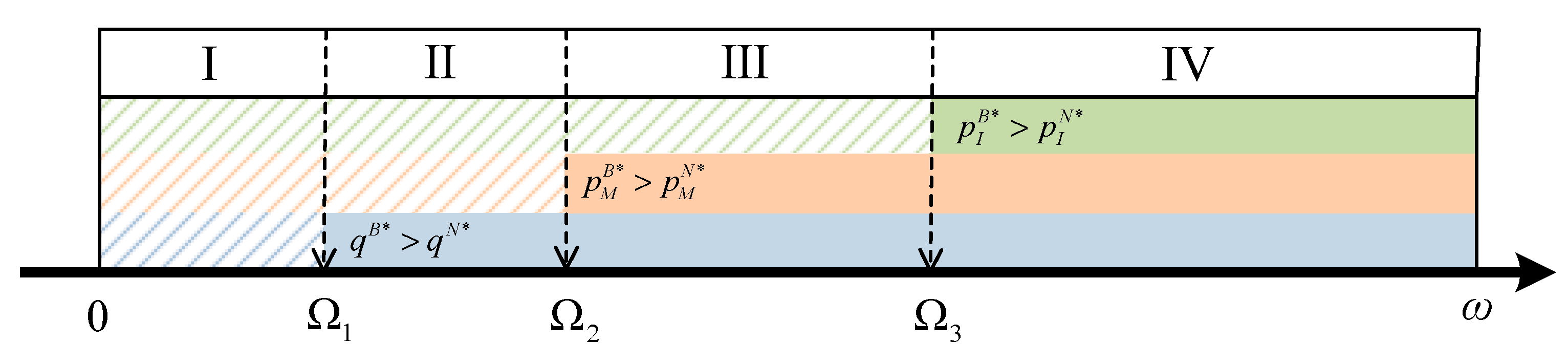
(1) The impact on the original product quality decision is that when  ${\Omega }_1<o<\omega$ , there is $q^{B*}>q^{N*}$ , otherwise, $q^{B*}\le q^{N*}$ . (2) The impact on the retail price of refurbishment is that when ${\Omega }_2<o<\omega$ , $p_M^{B*}>p_M^{N*}$ , otherwise, $p_M^{B*}\le p_M^{N*}$ ; and when ${\Omega }_3<o<\omega$ , $p_I^{B*}>p_I^{N*}$ , otherwise, $p_I^{B*}\le p_I^{N*}$.

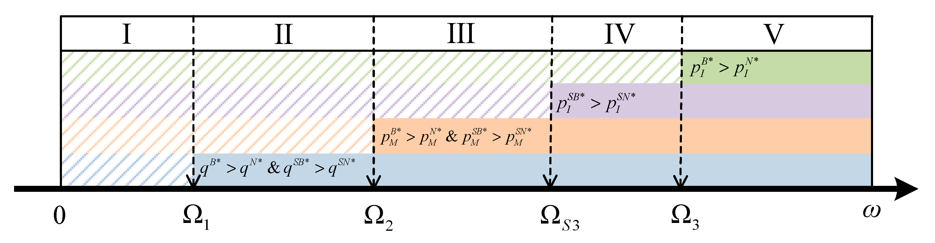
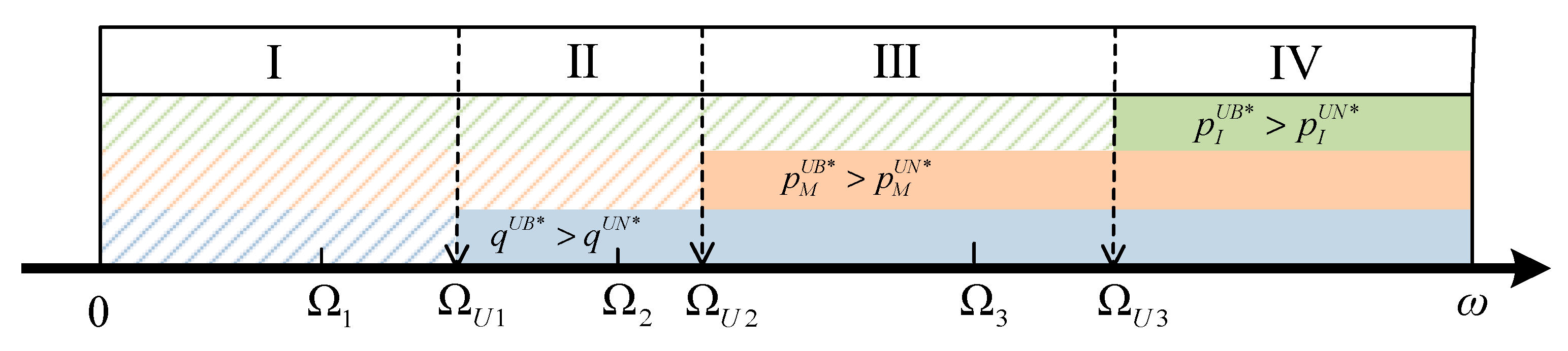
According to Proposition 1, a unifying inference is that when BT adoption leads to strong brand market competitiveness or a substantial increase in consumer stickiness, competition in the quality dimension will intensify, but competition in the price dimension will be effectively mitigated. In contrast, when BT achieves less strong brand competitiveness, different competitive circumstances are likely to emerge. The validity of this proposition relies on the premise that BT enhances brand competitiveness or consumer stickiness, but in reality, consumers’ acceptance of refurbished products varies. For instance, some consumers pay more attention to price rather than quality traceability and are unconcerned about the quality information certified by BT. Such cases conflict with the aforementioned expected proposition. The specific impact of BT on competitive intensity can be summarized in Figure 1 by further comparing the thresholds.

As shown in Figure 1, the impact of BT on the intensity of competition in the quality and price dimensions in the refurbishment market can be divided into the following four regions:

(1) In region I, when the competitiveness enhanced by BT is extremely low ($0\le o<{\Omega }_1$), the intensity of competition in the quality dimension decreases, but the intensity of competition in the price dimension increases (manifested by price reductions in both M and I).

(2) In region II, when BT raises less competitiveness (${\Omega }_1\le o<{\Omega }_2$), the intensity of competition in both the quality and price dimensions increases (as evidenced by price reductions in both M and I).

(3) In region III, when BT raises a relatively high competitiveness (${\Omega }_2\le o<{\Omega }_3$), the intensity of competition in the quality dimension is further increased but competition in the price dimension is mitigated (as evidenced by M raising the price and I lowering the price).

(4) In region IV, when BT brings great market competitiveness (${\Omega }_3\le o\le \omega$), the intensity of competition in the quality dimension increases dramatically, but the intensity of competition in the price dimension decreases significantly (both M and I raise prices).

The reason for this result is that raised brand competitiveness essentially means a lower rate of brand decay. After the BT implementation, the quality of M’s refurbishment can be disclosed truthfully and credibly. The improvement of the quality of refurbishment will effectively work on the brand’s goodwill. Therefore, a wise M will improve the quality of the refurbished product by investing more in the quality of the original product. On the contrary, as BT enhances M’s brand competitiveness, competition in the price dimension is mitigated. This is because with BT’s further increased brand premium, both M and I will increase their refurbishment prices to capture higher revenues.

Further analysis of the cross-price elasticity of demand can lead to a better understanding of the impact of price changes on competition. First, define the cross-elasticity coefficient of demand for M with respect to the price of I ${\eta }_{MI}^i={\displaystyle \frac{\mathrm{d}{Q}_M^i}{\mathrm{d}{p}_I^i}}{\displaystyle \frac{p_I^i}{Q_M^i}},i\in \{N,B\}$, which reflects the sensitivity of M’s demand to $p_I^i$ changes. Similarly, the cross-elasticity coefficient of the demand for I with respect to the price of M is ${\eta }_{IM}^i={\displaystyle \frac{\mathrm{d}{Q}_I^i}{\mathrm{d}{p}_M^i}}{\displaystyle \frac{p_M^i}{Q_I^i}},i\in \{N,B\}$, which reflects the sensitivity of I’s demand to $p_M^i$ changes.

Proposition 2. 

(1) When M does not implement BT, when $\chi <1/2$ there is ${\eta }_{MI}^N>{\eta }_{IM}^N$ ; otherwise, there is ${\eta }_{MI}^N\le {\eta }_{IM}^N$ . (2) When BT is implemented, when $\chi <\phi /(1+\phi )$ there is ${\eta }_{MI}^B>{\eta }_{IM}^B$ ; otherwise, there is ${\eta }_{MI}^B\le {\eta }_{IM}^B$.

Proposition 2 shows that without BT, the demand for M is more sensitive to changes in the retail price of I when her market share is smaller. Conversely, when M occupies a larger market, she will be less sensitive to changes in I’s price. The first impact of BT can be obtained from this relationship by $\phi /(1+\phi )<1/2$. That is, the implementation of BT makes the demand for M resistant to changes in the retail price of I over a wider market. This side-step validates the conclusion that the implementation of BT has mitigated price competition to some extent. By comparing the cross-price elasticity of the same demand in different scenarios, it can be obtained that ${\eta }_{MI}^B<{\eta }_{MI}^N$ and ${\eta }_{IM}^B>{\eta }_{IM}^N$. This reveals the second impact of BT implementation. The implementation of BT by M not only makes its demand less sensitive to changes in I’s price, but also makes I’s demand more sensitive to changes in M’s price. In other words, the implementation of BT not only mitigates the impact of price competition from rivals but also improves M’s market competitiveness.

5.2. Impact of BT Implementation on the Brand and Consumers

Proposition 3. 

(1) The impact of BT implemented on the brand is, when  ${\Omega }_4<o<\omega$ , there is $G_s^{B*}>G_s^{N*}$ ; otherwise, $G_s^{B*}\le G_s^{N*}$ . (2) The impact of BT implementation on the price–quality ratio of refurbished products obtained by consumers is as follows: when purchasing a refurbished product from M, there is $\frac{q_M^{B*}}{p_M^{B*}}>\frac{q_M^{N*}}{p_M^{N*}}$ when $\mu <\epsilon$ and $o<\left(\epsilon -\mu \right){\xi }_M$ , otherwise, $\frac{q_M^{B*}}{p_M^{B*}}\le \frac{q_M^{N*}}{p_M^{N*}}$ . When purchasing a refurbished product from I, $\frac{q_I^{B*}}{p_I^{B*}}<\frac{q_I^{N*}}{p_I^{N*}}$ when ${\Omega }_5<o\le \omega$ , otherwise, $\frac{q_I^{B*}}{p_I^{B*}}\ge \frac{q_I^{N*}}{p_I^{N*}}$.

Proposition 3 suggests that (1) intuitively, for M, the implementation of BT is beneficial to brand building only when the adoption of BT brings sufficient competitiveness to M or significantly enhances consumer stickiness. (2) For consumers, the implementation of BT by M does not necessarily lead to more cost-effective refurbished products, whether purchased from M or from I. If consumers buy refurbished products from M, counterintuitively, they will only obtain a more cost-effective refurbished product if the DRQE is small and the competitiveness gains from the implementation of BT by M are not significant. Otherwise, consumers will get refurbished products at a higher price, making it less cost-effective. This is because DRQE not only enhances the quality of refurbished products, but also maximally raises brand goodwill in the trustworthy environment achieved through BT. Under the brand premium effect based on BT, the improvement of refurbishment quality is less than the improvement of refurbishment price. And when consumers buy refurbished products from I, if the competitiveness brought by M’s implementation of BT is too high, the prices of the refurbished products sold by I increase more than their quality has improved. As a result, the cost-effectiveness of the refurbished products that consumers get from I will also be reduced. Conversely, competition in the price dimension becomes intense, and consumers are able to obtain refurbished products that are more cost-effective.

5.3. Impact of BT Implementation on the Interaction of the Two Reference Behaviors

In order to analyze the impact of BT implementation on the interaction between RQB and RPB, firstly, it is necessary to obtain the equilibrium outcomes when consumer RPB is neglected under the two scenarios where M does not implement and where BT is implemented (corresponding to scenario N0 and scenario B0, respectively). Then, the obtained equilibrium outcomes are compared with the corresponding equilibrium outcomes under scenarios N and B, respectively. The results are shown in Propositions 4 and 5.

Proposition 4. 

(1) When M does not implement BT, the impact of RPB on the optimal strategies is $q^{N*}>q^{N0*}$ , $p_M^{N*}>p_M^{N0*}$ , $p_I^{N*}>p_I^{N0*}$ . (2) When BT is implemented, the impact of RPB on the optimal strategies is $q^{B*}>q^{B0*}$ , $p_M^{B*}>p_M^{B0*}$ and $p_I^{B*}>p_I^{B0*}$.

Proposition 4 shows that, regardless of whether BT is implemented or not, consumers’ RPB promotes M to improve the quality of the original product and subsequently increases the retail price of the refurbished product. In other words, the presence of consumer RPB and RQB increases competition in the quality dimension but reduces competition in the price dimension. Further analysis indicates that when ${\Omega }_6<o<\omega$, $q^{B*}-q^{B0*}>q^{N*}-q^{N0*}$, else, $q^{B*}-q^{B0*}\le q^{N*}-q^{N0*}$. And while ${\Omega }_7<o<\omega$, $p_M^{B*}-p_M^{B0*}>p_M^{N*}-p_M^{N0*}$, otherwise, $p_M^{B*}-p_M^{B0*}\le p_M^{N*}-p_M^{N0*}$. In addition, while ${\Omega }_8<o<\omega$, $p_I^{B*}-p_I^{B0*}>p_I^{N*}-p_I^{N0*}$, otherwise, there is $p_M^{B*}-p_M^{B0*}\le p_M^{N*}-p_M^{N0*}$. This implies that the implementation of BT further amplifies the impact of RPB when BT leads to stronger brand competitiveness.

Proposition 5. 

The impact of consumers’ reference behaviors is summarized in 

Table 1. The impact of consumers’ reference behaviors.

RQB (QB)		${\delta }_M\le {\delta }_I$			${\delta }_M>{\delta }_I$
	N		$\mathrm{Any}{\xi }_M>0$		$0<{\xi }_M<{\underset{\_}{\xi }}_M$	${\underset{\_}{\xi }}_M\le {\xi }_M<{\overline{\xi }}_M$	${\xi }_M\ge {\overline{\xi }}_M$
		DRQE	$+$		$+$	$+$	$-$
		IRQE	$-$		$-$	$+$	$+$
		RQB	$\frac{{\delta }_I\epsilon }{{\delta }_M}<\mu <\overline{\mu }$	$\mu \ge \overline{\mu }$	$\mu >\frac{{\delta }_I\epsilon }{{\delta }_M}$
			$-$	$+$	$+$
	B	DQE	$+$		$+$
		IQE	$-$		$+$
		QB	$\mu >\frac{{\delta }_I\epsilon }{{\delta }_M}$
			$+$
RPB		$\frac{\gamma }{2}<\beta \le \gamma$			$\beta >\gamma$
	N	$\mathrm{Any}\nu >0$			$\nu <\overline{\nu }$		$\nu \ge \overline{\nu }$
		$-$			$-$		$+$
	B	$\mathrm{Any}\nu >0$			$\nu <\overline{\nu }$		$\nu \ge \overline{\nu }$
		$-$			$-$		$+$

Notes: $+$ represents positive impact, $-$ represents negative impact. Where specific expressions of $\overline{\mu }$, ${\underset{\_}{\xi }}_M$, ${\overline{\xi }}_M$ and $\overline{\nu }$ are presented in Appendix B.

.

First, the impact of RQB (QB) depends on the M’s degree of refurbishment with respect to I. (1) If M’s degree of refurbishment is low, when she does not implement BT, then the DRQE will always have a positive impact, while the IRQE will always show a negative impact. And only when DRQE dominates goodwill ($\mu$ is larger) does RQB generate a positive impact; otherwise, RQB generates a negative impact. When M implements BT, it enhances the positive impact of DQE. QB will eventually generate a positive impact, even if $\mu$ is not as large. This can be interpreted as the BT at low levels of refurbishment of M reduces the adverse effects of quality competition on goodwill. (2) And when the degree of M refurbishment is high, the impact of DEQE and IRQE is further moderated by the degree of association between reference quality and goodwill. When M does not implement BT, the low degree of association incentivizes the positive impact of DRQE, whereas the high degree of association causes DRQE to exhibit a negative impact. In contrast, IRQE has the opposite impact. Combining the effects of RQB-induced DRQE and IRQE shows that RQB will always have a positive effect when BT is not implemented. When BT is implemented, surprisingly, both DQE and IQE have a positive impact, which allows QB to achieve a positive impact on goodwill at all times. This is because M will always produce refurbished products of higher quality than I’s refurbished products, thus exploiting the positive impact of quality on goodwill to the fullest extent possible with BT.

Secondly, the ultimate impact of RPB is influenced by both the extent to which RPB affects goodwill and the degree of association between the reference price and goodwill. (1) When consumers’ RPB does not dominate demand, RPB consistently has a negative effect on M and I. BT implementation serves to mitigate this negative effect. This result is derived from the fact that the brand premium effect from BT raises consumers’ price expectations. (2) And when consumers’ RPB dominates demand, RPB will show a positive impact only when the reference price and goodwill are highly correlated. Otherwise, RPB will show a negative influence. Additionally, BT implementation will enhance the positive impact of RPB and mitigate the negative impact of RPB to some extent. This is because the increase in goodwill makes consumers willing to pay a higher price than M and I’s pricing only if the reference price and goodwill are highly correlated. The presence of BT leverages the brand premium effect to further increase consumers’ willingness to pay by enhancing goodwill, thus widening the gap between price and reference price when the reference price is high and narrowing the gap between the two when the reference price is low.

6. Numerical Examples

This section further explores the impact of different exogenous environmental changes on the implementation of BT through numerical analyses, while validating the analytical results of the previous section. Based on impact studies of BT implementation in monopoly or supply chain environments, such as Niu et al. [64] and Ma et al. [8], in conjunction with the relevant assumptions in the competitive environment of the refurbished market explored in this paper, the values of the basic parameters are set as follows: $\beta =0.5$, $\gamma =0.1$, $\chi =0.3$, $\theta =0.5$, ${\xi }_M=0.3$, $v=0.3$, $\omega =0.3$, $\rho =0.1$, $k=0.2$, $o=0.1$, $\phi =0.5$, $F=0.2$.

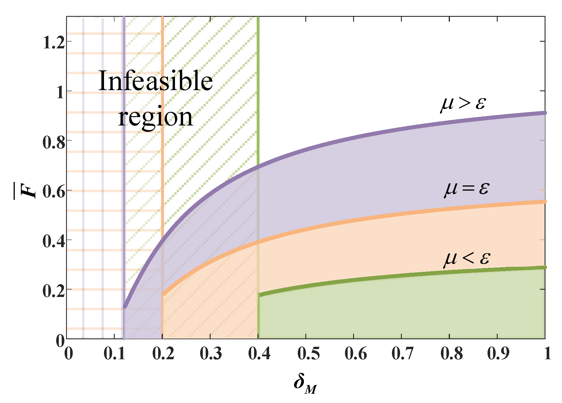
6.1. Market Conditions for M to Adopt BT

Figure 2 portrays the variation in the feasible range of BT for different size relationships of consumer DRQE and IRQE for different levels of refurbishment of M. First, the two determine the boundary of BT implementation to some extent. When IRQE dominates the brand, i.e., $\mu <\epsilon$, M’s willingness to implement BT is low. She will choose to adopt BT only when the degree of refurbishment is large and the cost of BT implementation is low. What can verify this conclusion is that Nike, in its official refurbished product sales, introduced a quality traceability system based on BT to disclose the repair records and performance test results of the refurbished products in a trustworthy manner. Due to the high degree of refurbishment (close to the standards of new products) and the relatively controllable implementation cost of BT, Nike significantly enhanced consumers’ trust in the quality of official refurbished products through this technology. Thus, it consolidated its brand advantage in the highly competitive refurbished market and effectively countered the competition from the I [65]. As DRQE increases, M will expand the scope of BT implementation. When DRQE exceeds IRQE, M will choose to implement BT even if the degree of refurbishment is low. And as the degree of refurbishment increases, M will also gradually increase the upper cost limit of acceptable BT implementation. The specific reasons are as follows: When DRQE is weak, the competition between M and I in terms of quality is a key factor affecting brand goodwill. At this time, improving the refurbishment level to optimize product quality is more effective in avoiding potential goodwill losses caused by IRQE than disclosing quality through BT. When DRQE dominates the goodwill, even if the refurbishment level is low, as long as the original quality of M is high enough, in the trustworthy quality environment constructed by BT, brand goodwill can be effectively enhanced.

6.2. Impact of BT Implementation Under Different DRQEs and IRQEs

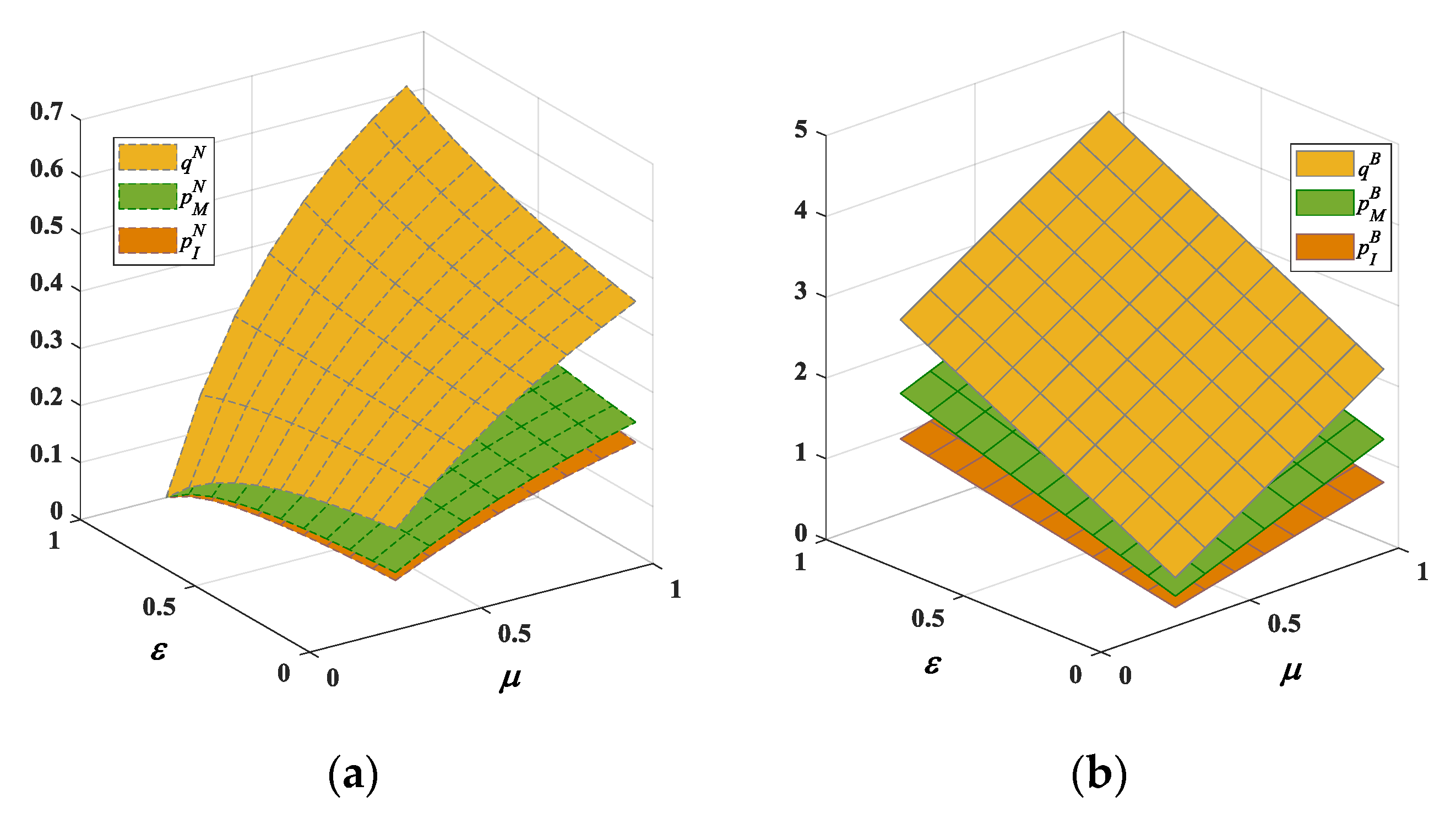
With the help of Figure 3 to illustrate the impact of the different sizes of DRQE and IRQE on the implementation of BT, its impact on competition in the refurbishment market can be obtained.

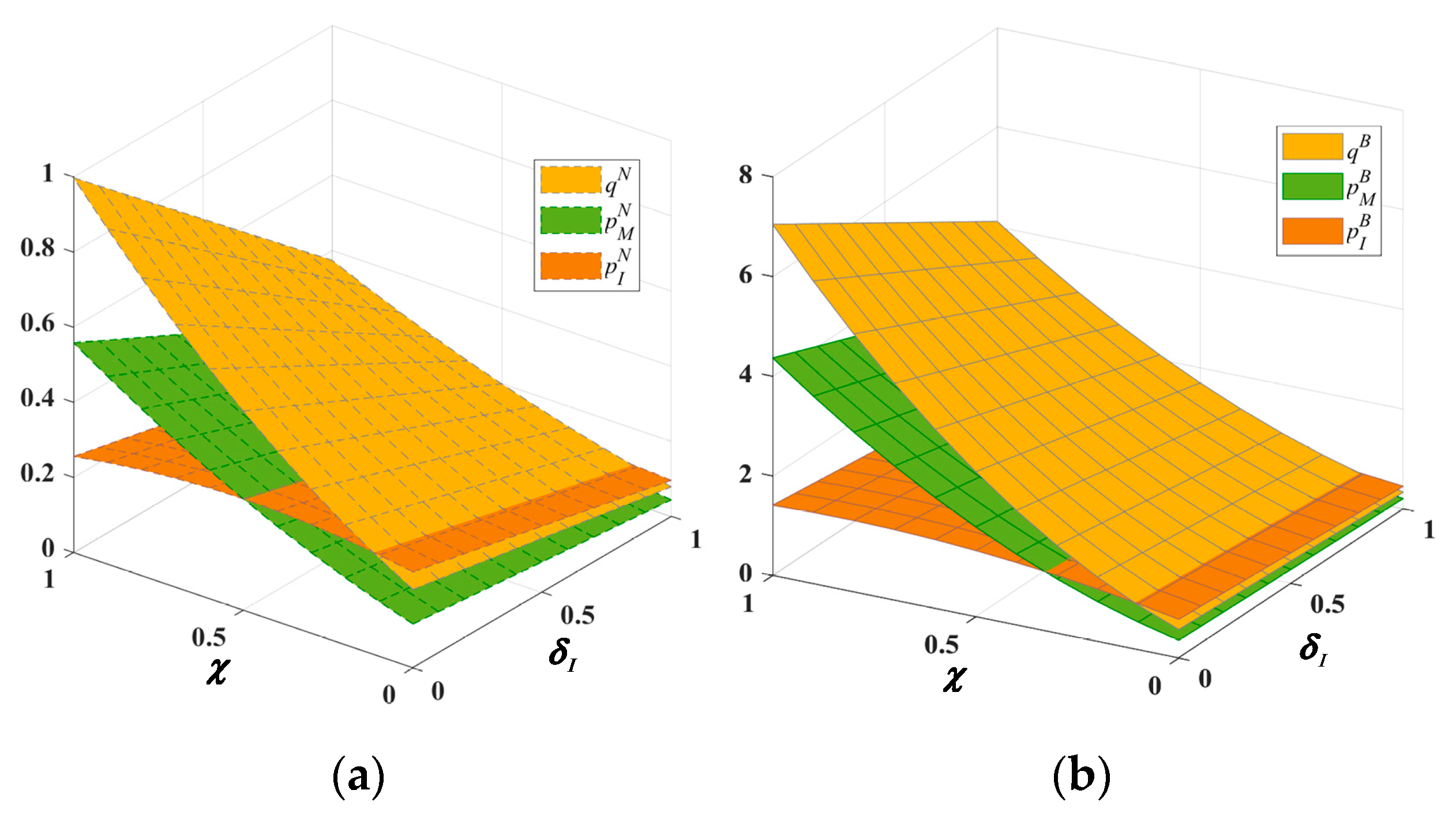
Figure 3a shows that the different sizes of DRQE and IRQE present non-monotonic impacts on the optimal decision when M does not adopt BT. Specifically, an increase in DRQE will always intensify competition in the quality dimension but mitigate competition in the price dimension. And the impact of IRQE depends on its size in relation to DRQE. When IRQE dominates goodwill, the optimal decisions all decrease with its increase. But when DRQE dominates, the optimal decisions show the opposite change.

When M implements BT, the original DRQE becomes the direct impact of M’s refurbished product quality on goodwill (DQE) and IRQE becomes the indirect impact of M’s competition with I’s quality dimension on goodwill (IQE). At this point, the different sizes of the two effects present monotonic impacts on the optimal decision. Whichever effect becomes larger intensifies the competition in the quality dimension but mitigates the competition in the price dimension (e.g., Figure 3b). This is the result of the credible quality disclosure and enhanced brand premium effect achieved by BT and again validates the role of BT on competition in Proposition 2.

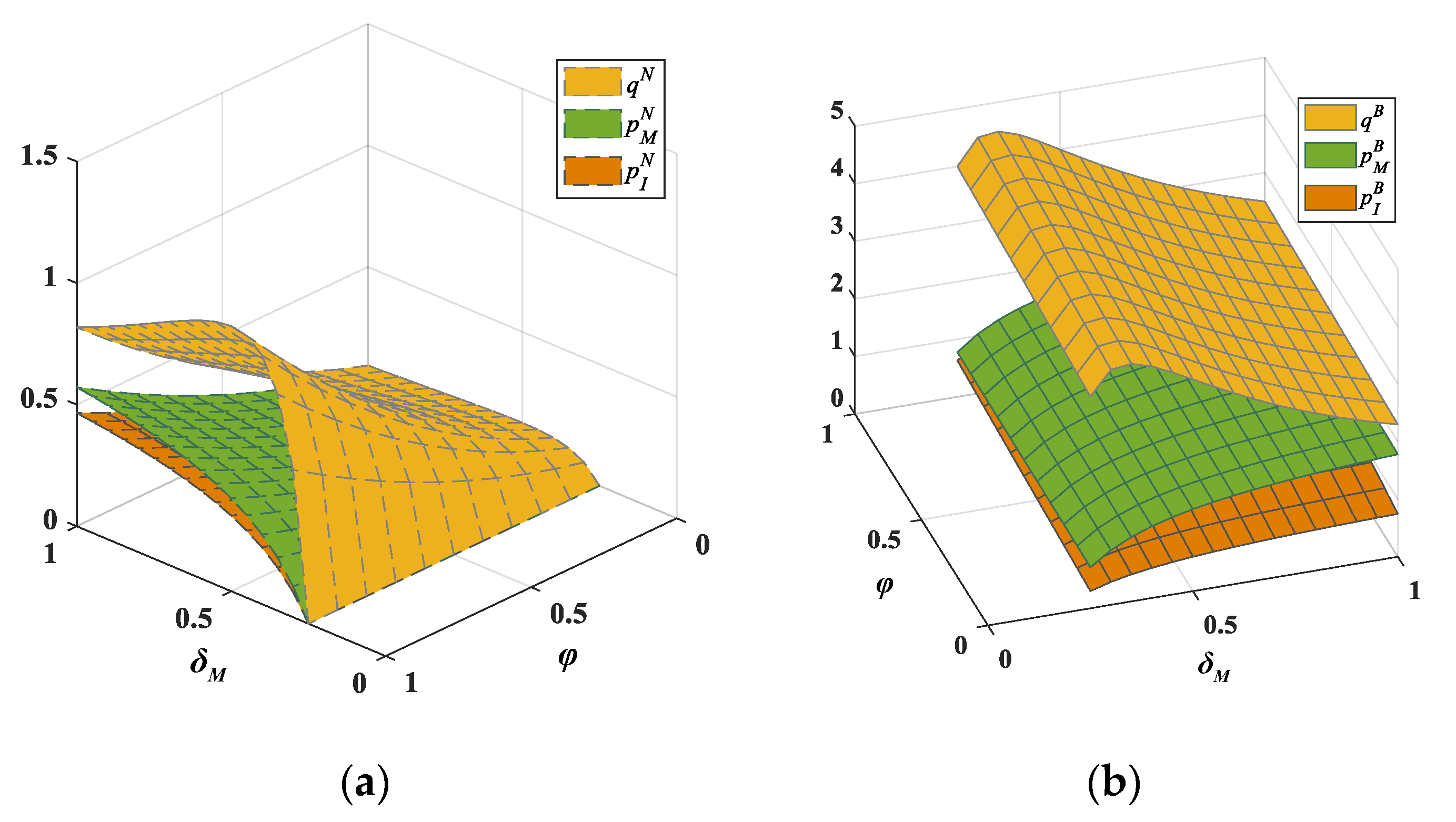
6.3. Impact of BT Implementation Under Different Levels of M’s Refurbishment Degree and Consumer Trust

A comparison of Figure 4a,b shows that an increase in consumer trust always intensifies quality dimension competition but alleviates price dimension competition, regardless of whether M chooses to adopt BT or not. The degree of M’s refurbishment has a non-monotonic impact on quality dimension competition but always alleviates price dimension competition. Specifically, M always improves the quality of the original product as consumer trust increases, but eventually the quality of the original product tends to increase and then decrease as M’s degree of refurbishment increases. While the former is intuitive, the latter can be explained by the fact that a high degree of refurbishment allows M to obtain a higher quality of refurbished products without setting a higher quality of original products. The increase in trust can essentially increase consumers’ willingness to pay, which allows companies to set higher prices based on the goodwill brought about by the quality improvement. However, since consumer distrust of I still exists, I will choose to increase the retail price of refurbished products even further with the increase in consumer trust. In this way, I can take advantage of the brand premium effect brought about by M’s implementation of BT and ride on M’s goodwill enhancement from the original product’s quality improvement in a trustworthy environment.

6.4. Impact of BT Implementation Under Different Market Segments and I’s Refurbishment Degree

As can be seen from Figure 5a,b, the higher the initial market share of M in the refurbishment market, whether BT is implemented or not, the more intense is the competition in the quality dimension, while the competition in the price dimension is smoother. And this trend becomes more pronounced as the degree of refurbishment of I decreases. This can be interpreted as M’s high share in the refurbished market allows it to gain more demand from the goodwill enhancement brought about by quality improvement, but it also promotes free-riding behavior of I. This allows I to produce higher quality refurbished products even when the degree of refurbishment is low, thus increasing competition in the quality dimension. And with consumer RQB, given that high brand goodwill raises consumers’ price expectations, sensible M’s and I’s take advantage of this consumer behavior to raise refurbishment prices. This, on the contrary, makes the competition in the price dimension mitigated. The effect of BT implementation is, on the one hand, to increase the effect of quality inputs to goodwill through credible quality disclosure, thus further intensifying competition in the quality dimension. On the other hand, with the brand goodwill enhanced by increased quality, M and I are further induced to increase the pricing of refurbished products through their brand premium effect, which mitigates the competition in the price dimension.

6.5. Effectiveness of BT Implementation at Different Levels of Refurbishment and Trust

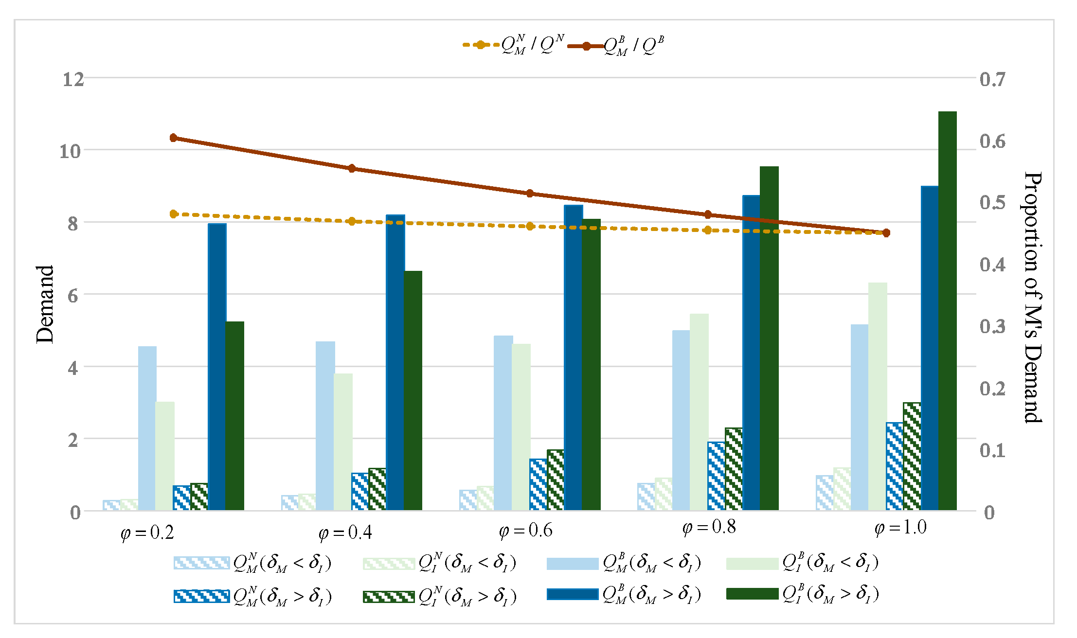
From Figure 6, firstly, it can be found that in the same scenario and with the same level of consumer trust, a higher degree of refurbishment of M always brings higher demand to both M and I. This is due to the fact that a higher degree of refurbishment of M always positively incentivizes it to improve the quality of the original product to enhance goodwill. This will expand the total market size, thus benefiting both M herself and the free-rider I. This is consistent with our observations of the Apple refurbished market. In a refurbished market where consumers have little trust in both Apple’s official and Back Market offerings, Apple’s official refurbished products have gained favorable market responses thanks to their high-standard refurbishment process, brand endorsement and official warranty. This trend not only drives Apple to increase investment in new product innovation and quality improvement to strengthen its brand reputation but also creates revenue growth points for the Back Market through brand spillover effects [66]. Calculations show that the degree of refurbishment of M and I will not affect M’s final market share. Secondly, a side-by-side comparison of the two scenarios shows that the presence of BT promotes the demand for both M and I and ultimately leads to a higher market share for M. This is due to the fact that the BT application enlarges the overall market size, which in turn raises the market demand for M and I, respectively. In the process, as the adoption of BT allows M to gain full consumer trust while I remains questionable, the market demand for M will increase more than that for I, resulting in a higher final market share. It is for this reason that the increase in M’s final market share will weaken as consumers’ trust in I increases.

6.6. Effectiveness of BT Implementation with Different Reference Effects and Refurbishment Levels

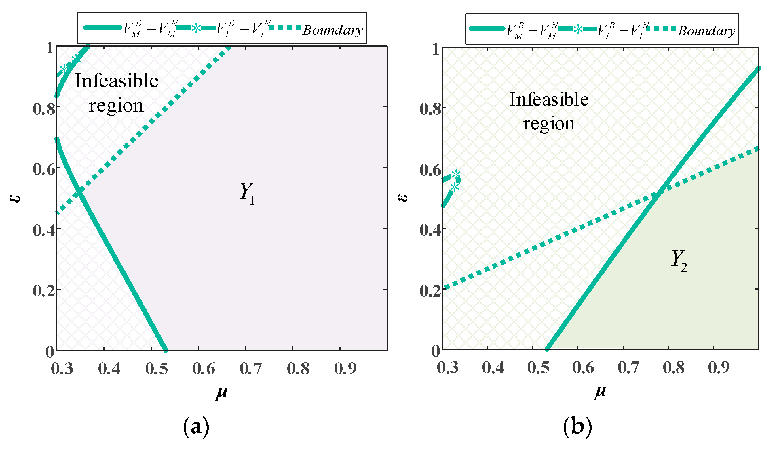
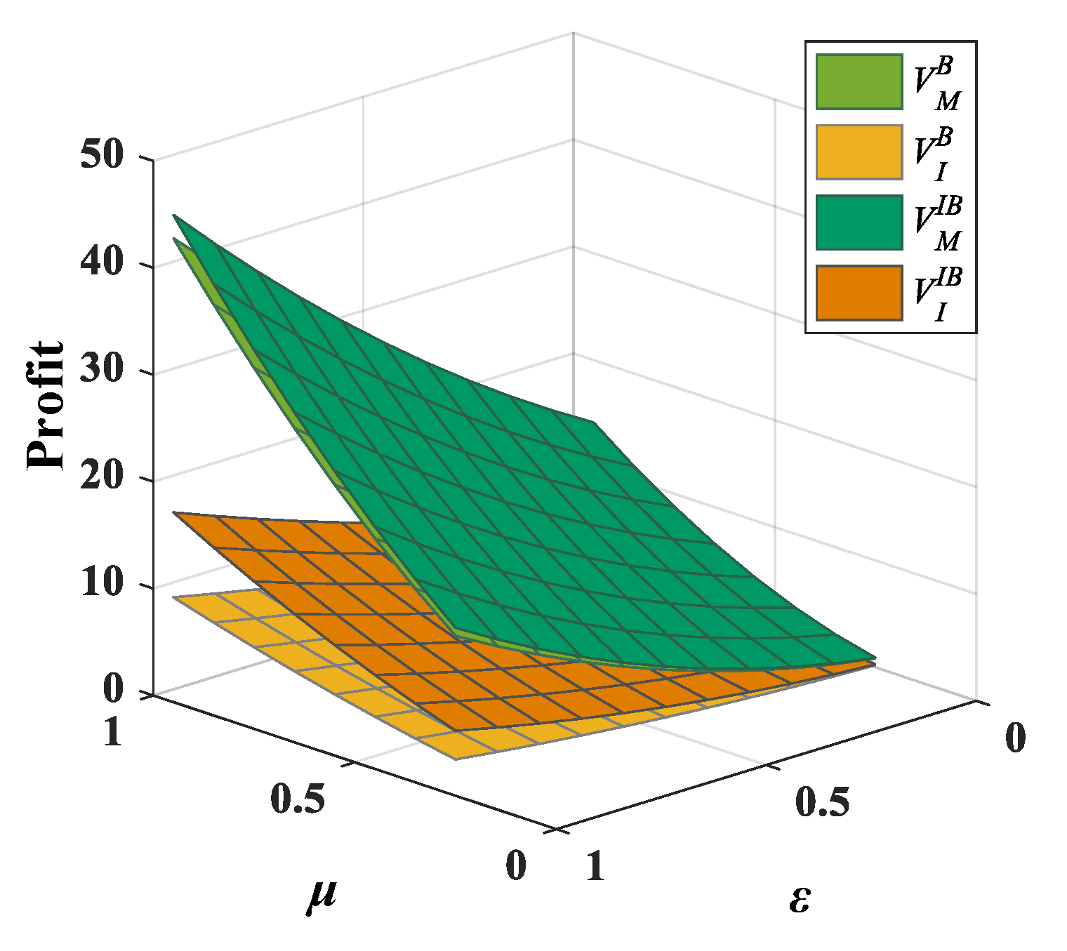
In the case where M implements BT, the impact of BT implementation on I’s profit could be obtained by classifying the degree of M’s refurbishment and the size of DRQE and IRQE triggered by the RQB. As shown in Figure 7a, region $Y_1$ (M with a high degree of refurbishment and a high DRQE) indicates that M’s implementation of BT will not only be profitable for itself, but will also increase the profitability of the competitor I. In this situation, the implementation of BT will merely serve as a promotional tool, aiming to enhance the brand reputation by increasing consumers’ trust in M. However, it cannot achieve the goal of combating I through its implementation. As shown in Figure 7b, in region $Y_2$ (when M’s refurbishment is low and DRQE is dominant), M’s implementation of BT will only benefit herself but disadvantage I. In this case, M’s implementation of BT can be used as a competitive tool against I in the refurbishment market. The reason for this is that M is more susceptible to damage from IDQE when it has a low level of refurbishment. Only when DRQE dominates is goodwill protected from damage through BT implementation. However, at this point, the profitability of I will be substantially lower as the goodwill is still low and the limited market size and lower brand premium under is not enough to compensate for the higher costs.

6.7. Effect of BT Implementation with Different Reference Effects and Refurbishment Levels

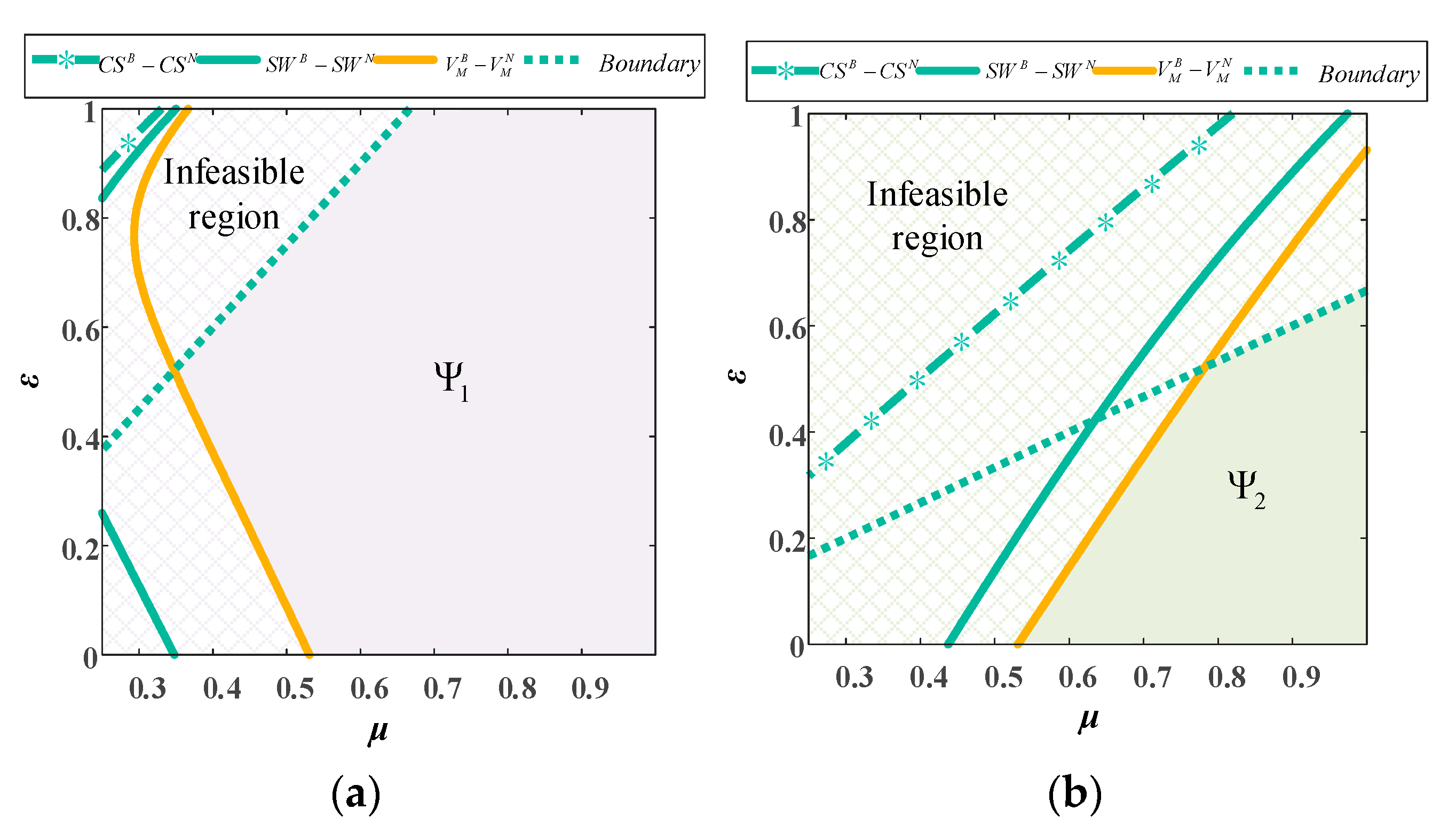
Figure 8 further analyses the impact of BT adoption on consumer surplus (CS) and social welfare (SW). It can be found that the implementation of BT always increases both CS and SW in the BT feasible region, as long as its implementation brings sufficient competitiveness to M. In Figure 8a, area ${\Psi }_1$ indicates that M, I, consumers and the whole society will be better off from the deployment of BT. This result is intuitive. Because, in conjunction with Figure 7a, when the refurbished level of M is high, the implementation of BT not only increases the profits of both M and I, but also enhances consumers’ willingness to pay due to the brand premium effect brought by BT. Under a reasonable pricing that takes into account RPB, the CS received by consumers increases, thereby bringing about higher SW. Whereas, when the refurbishment of M is low (as in Figure 7b), deploying BT will only result in higher CS and SW when DRQE is dominant (as in the ${\Psi }_2$ region). This is because, when M’s refurbishment level is low, only when DRQE dominates can M directly utilize the quality-enhancing effect on goodwill by implementing BT, avoiding the adverse effect of IRQE, and thus leading to an increase in its own profit. And at this point, although BT as a competitive tool reduces I’s profit, I’s profit loss is lower than M’s profit enhancement. And the presence of brand premium effect still leads to higher CS and therefore higher SW.

7. Extension

This section extends the benchmark model to validate the robustness of the findings and to obtain richer managerial insights in four ways: (1) I acts as a follower of M’s price setting in the refurbishment market (Scenario S), (2) both M and I implement BT (Scenario I), (3) M and I are subjected to different levels of consumer trust (Scenario F) and (4) M and I have different refurbishment costs (Scenario K).

7.1. I Acts as a Follower of M’s Price Setting in the Refurbishment Market (Scenario S)

Consider the following scenario: I chooses to set the retail price of his refurbished products after M sets the retail price of her refurbished products. For example, Amazon sets the price of the refurbished mobile phones based on the pricing of Apple’s refurbished mobile phones. In this case, the order of the game is that M decides the quality of the original product and the retail price of the refurbished product first, and I decides the retail price of the refurbished product. The superscripts $Si,i\in \{N,B\}$ denote the two new scenarios of not implementing and implementing BT under scenario S, respectively.

Firstly, upon comparison, it is found that $q^{SB*}>q^{B*}$ and $q^{SN*}>q^{N*}$. Further comparing the thresholds of competitive regions under scenario S and the baseline model, there is the following relationship: ${\Omega }_1={\Omega }_{S1}<{\Omega }_2={\Omega }_{S2}<{\Omega }_{S3}<{\Omega }_3$. Figure 9 presents more clearly the effect of BT deployment on competition intensity in scenario S.

This result suggests that I, when acting as a price follower in the refurbishment market, raises the retail price of refurbished products before the implementation of BT brings about greater competitive intensity. This move also further intensifies competition in the quality dimension but mitigates competition in the price dimension to a greater extent as the intensity of competition raised by the implementation of BT by M gradually increases. The reason for this is that when I, as a follower in the refurbishment market, is able to increase its pricing flexibility and plunder the BT-expanded market with the help of more appropriate refurbishment price-setting, this forces M to discourage I’s free-riding behavior and price competition by further improving the quality of the original product, thus driving quality competition in the refurbishment market. In real production scenarios, M need to maintain a cautious attitude when enhancing the quality of original products. On one hand, quality improvement often requires significant adjustments such as product design reengineering and replacement of key components, which are constrained by existing production technologies. On the other hand, as the quality level of the original products approaches the technological limit, the marginal cost will increase significantly, and it becomes necessary to fully consider the balance between input and output.

7.2. Both M and I Implement BT (Scenario I)

In practice, it is also common for I to deploy BT to trace and disclose quality information of refurbished products. For example, the Pai Pai refurbished platform under the JD Group carries out BT-bases quality certification when selling refurbished mobile phones and other household electronic appliances [43]. At this point, the demand function after the implementation of BT of I transforms into

$$Q_I^{IB}(t)=\left(1-\chi \right)\theta \sqrt{G^{IB}(t)}-\beta \left(p_I^{IB}(t)-v\sqrt{G^{IB}(t)}\right)+\gamma p_M^{IB}(t)$$

(9)

Comparing the equilibrium outcome under scenario I with that under the benchmark model B shows that $q^{IB*}>q^{B*}$, $p_M^{IB*}>p_M^{B*}$, $p_I^{IB*}>p_I^{B*}$. The emergence of this result implies that competition in the quality dimension will be further intensified and competition in the price dimension will be further mitigated. The former is due to the fact that both M and I implement BT to truthfully disclose the quality of their respective refurbishments. A wise M will further improve the quality of the original product to improve its refurbished product in order to gain a competitive advantage. This will cause I to produce higher quality refurbished products with the same level of refurbishment, thus intensifying competition in the quality dimension. In addition, the higher quality of the refurbished product brings higher goodwill, which will drive the retail price of the refurbished product up further due to the brand premium effect achieved by BT. The changes in firm profits under Scenario I are summarized in Figure 10.

Furthermore, comparing the profits of the firms in scenarios I and B indicates that when I also implements BT, it not only improves his own profits, but also further improves the profits of M. And the degree of profit enhancement increases with the increase in DRQE and IRQE. This is attributed to the more consumer-trusted trading environment jointly created by M and I implementing BT. Despite the increased competition in the quality dimension, brand goodwill is also further enhanced through the improved quality of refurbished products. This not only results in higher brand premium effects and higher retail prices for refurbished products, but also expands the overall market size, enabling both M and I to capture more demand in a larger potential market.

7.3. M and I Are Subjected to Different Levels of Consumer Trust (Scenario F)

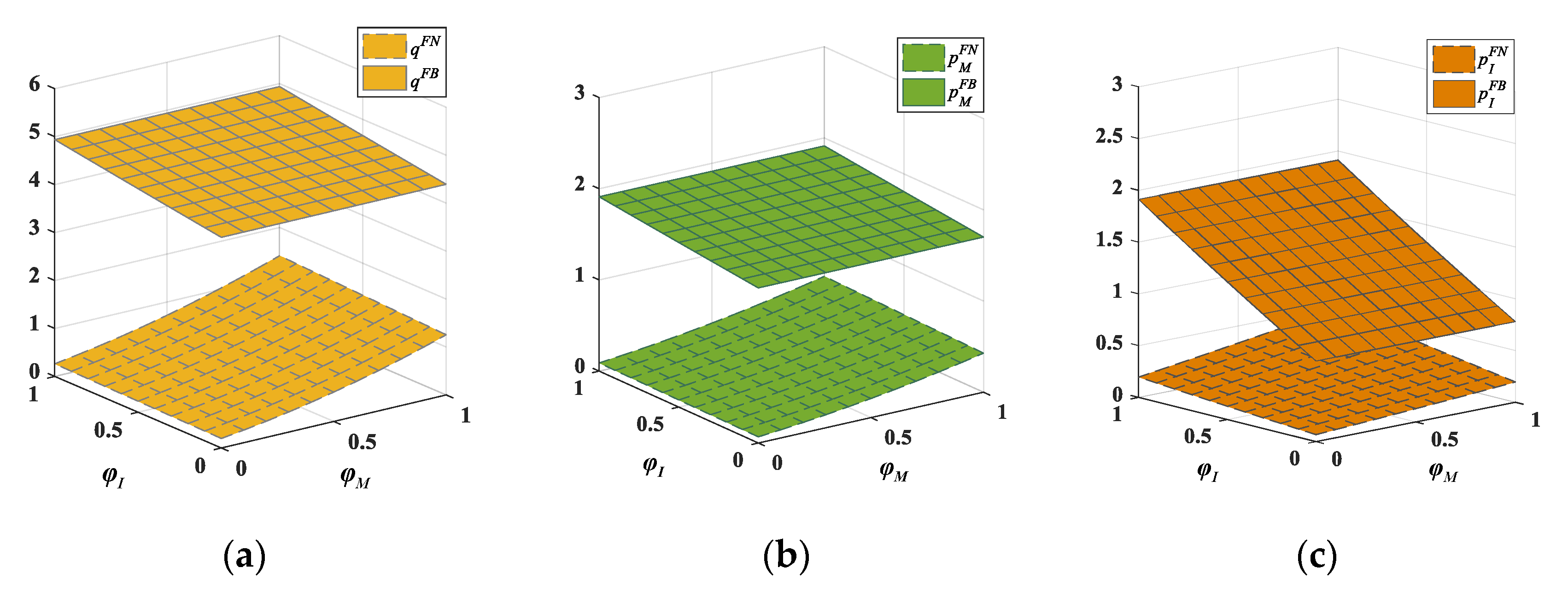
In the benchmark model, we assume that consumers trust both M and I with $\phi$. In fact, M and I are inconsistently trusted by consumers due to their different market positions, market sizes, duration of operation, business conditions, etc. [67]. For this purpose, it is assumed that consumers trust M and I with ${\phi }_M$ and ${\phi }_I$, respectively. At this point, the impact of BT implementation on competition is summarized in Figure 11 and Figure 12.

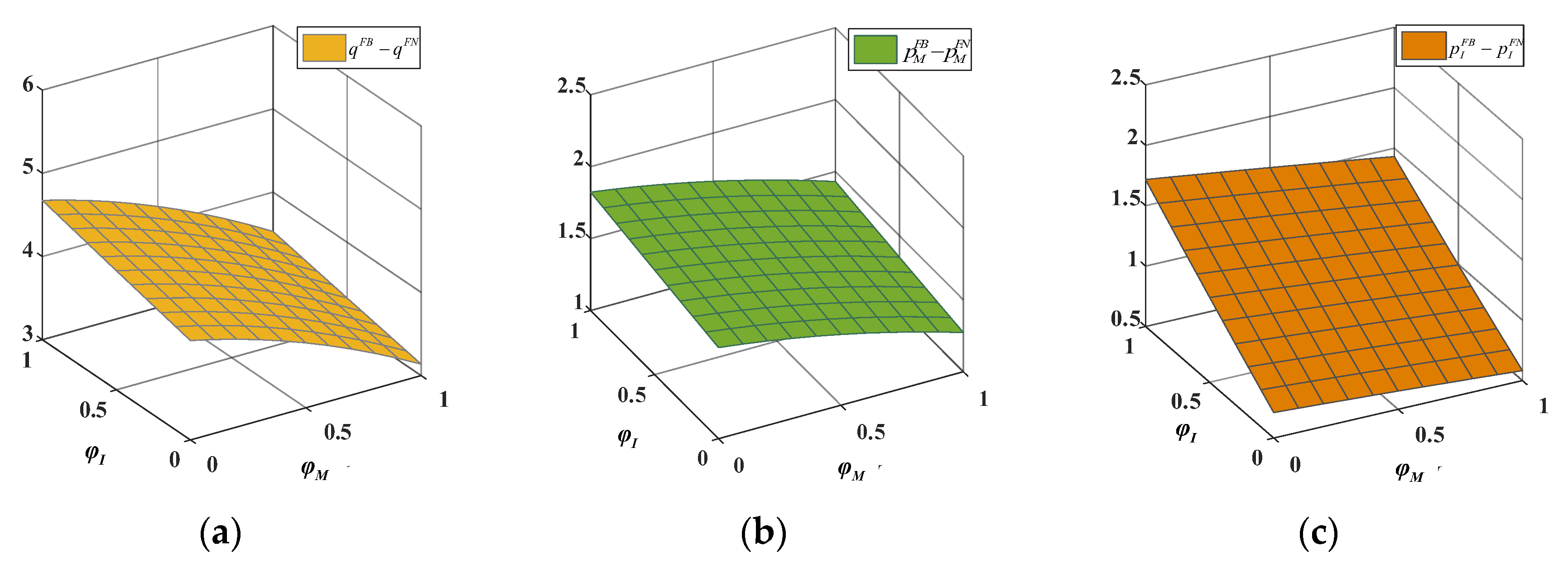
Consistent with the results of the main model, the implementation of BT intensifies competition in the quality dimension but mitigates competition in the price dimension, even if consumers have different levels of trust in M and I (as shown in Figure 11). Further analyzing the changes in the two dimensions according to Figure 12 shows that competition in the quality dimension is further intensified as consumers’ trust in M decreases and trust in I increases (Figure 12a). This is because M is facing a crisis of trust in the consumer market, and improving the quality of the original product to improve the quality of the refurbished product can recoup her own potential market loss by improving brand goodwill. And the retail price competition between M and I’s refurbished products is further mitigated with the decrease in consumer trust in M and the increase in trust in I (Figure 12b,c). This can be interpreted as the brand trust established by BT maximizes the effect of M’s improved refurbished product quality on goodwill enhancement. With the brand premium effect brought by BT, it pushes the market price of refurbished products up.

7.4. M and I Have Different Refurbishment Cost (Scenario K)

This section assumes that the refurbishment cost coefficients of M and I are $k$ and $\left(1+\sigma \right)k$, respectively. Where $\sigma <0$ indicates that I has a lower refurbishment cost and $\sigma <0$ indicates that M has a lower refurbishment cost.

It is verified that when the refurbishment cost coefficients are inconsistent the firm’s optimal decision, M’s profit and CS do not change, and only I’s profit and SW decrease with the increasing refurbishment costs. Therefore, the conditions for BT adoption and the impact of BT implementation on competitive intensity, brands and consumers do not change. The robustness of the main model conclusions is again verified.

7.5. Price-Sensitive Heterogeneity (Scenario H)

In real life, when consumers purchase refurbished products from I, they tend to be more influenced by price advantages. However, when consumers purchase refurbished products from M, they may be more affected by brand effects and other non-price factors and thus are less sensitive to the pricing of refurbished products. Therefore, this article expands on the inconsistent price sensitivity of consumers towards refurbished products from M and I. We consider the scenario where consumers are more sensitive to the pricing of I ${\beta }_I=(1+\varsigma )\beta$, $\varsigma >0$ depicts the differences in consumers’ price sensitivity. We have modified the demand function of I as follows:

$$Q_I^H(t)=\left(1-\chi \right)\phi \theta \sqrt{G(t)}-\left(1+\varsigma \right)\beta p_I(t)+\gamma p_M(t)$$

(10)

Compared with the basic model, we have found $q^{HN*}>q^{N*}$, $q^{HB*}>q^{B*}$. In Scenario H, consumers are not sensitive to the price of the refurbished products of M. M will consider improving the original product quality to indirectly enhance the quality of the refurbished products. This move can help M increase brand goodwill, thereby raising the price of the refurbished products and directly obtaining higher profits, without worrying about a significant loss in demand. In terms of price dimension, $p_M^{HN*}>p_M^{N*}$, $p_I^{HN*}>p_I^{N*}$; $p_M^{HB*}>p_M^{B*}$, $p_I^{HB*}>p_I^{B*}$. Although consumers are sensitive to the price of the refurbished product from I, the high price strategy of M has left room for the IR to increase the price. Therefore, even if I raise the price moderately, he will not lose a large amount of demand.

As shown in Figure 13, compared with Proposition 1, we found that when considering the differences in consumers’ price sensitivity, BR intensified competition in the quality dimension within a smaller scope, but intensified price competition within a larger scope. The differences in consumers’ price sensitivity lead M to set a higher quality for the original product. And BT, with its technical characteristics of quality traceability, can fully convert the existing higher quality of M into brand goodwill, thereby effectively increasing the brand premium. In this context, the marginal motivation for M to further improve original product quality to obtain additional profits is significantly weakened. Therefore, the scope for strategic adjustments through which M improves the quality of the original product shrinks accordingly after the implementation of BT. In the price competition dimension, the implementation of BT enables M to gain complete trust from consumers for their refurbished products, which further widens the gap in consumers’ perception of quality between M and I. In this situation, I, in order to maintain market share, has to lower the price to attract consumers. And given that consumers are more price-sensitive to I, the implementation scope of I’s price reduction strategy also expands accordingly. The low-price competition behavior of I seized some potential consumers of M, forcing M to lower the price within a wider range.

8. Discussion and Conclusions

8.1. Discussion

The main objective of this paper is to explore how M can formulate operational strategies for refurbished products in the face of competition from I. The analysis incorporates consumer reference behaviors and introduces BT as a countermeasure to address consumer distrust in the quality of refurbished products. Building on this framework, the paper focuses on analyzing the impact of M’s implementation of blockchain on the competitive landscape in the refurbished market.

Existing research primarily focuses on the cannibalization effect of refurbished products on the market share of original products. Consequently, prevailing views suggest that by enhancing the quality of the original product to increase the complexity of the refurbishment process [32,34,50], raising the price of the refurbished products and lowering the price of the original products [27,68], etc., it is possible to effectively curb the competition from I. However, this paper shifts its research perspective to the direct competition between the refurbished product of M and that of IR. In this situation, the quality and price of refurbished products will be significantly influenced by the consumer reference quality effect. Furthermore, we have discovered an interesting result. For instance, the implementation of BT does not always harm I. When the refurbishment level of M is high and the DRQE is large, the implementation of BT can simultaneously promote the demand and profit growth of both M and I. This is because the implementation of M enhances brand reputation by building consumers’ trust in M’s refurbished products, thereby expanding the overall market demand.

8.2. Conclusions

As the pace of product updates continues to accelerate, the refurbishment market has become highly visible. In the context of the refurbished market, this paper constructs a duopoly competition model consisting of a brand manufacturer M and an independent refurbisher I. At the same time, considering consumers’ RQB and RPB, it explores the impact of M’s implementation of BT to disclose the quality of refurbished products on the competition in the refurbished market. The main findings of this paper are as follows:

(1)

The cost threshold for M to implement BT depends on the relative size of the DRQE and IRQE triggered by the consumer RQB and is moderated by the degree of M’s refurbishment. When IRQE dominates brand goodwill, BT is adopted only when the degree of refurbishment is large and the cost of BT implementation is low. When DRQE exceeds IRQE, M chooses to implement BT to disclose the true refurbishment quality even if her refurbishment degree is low. And as the degree of refurbishment increases, M also gradually raises the upper limit of the acceptable BT implementation cost. This result stems from the combined influences of DRQE and IRQE on brand goodwill.

(2)

From the competition point of view, when the implementation of BT can bring high enough market competitiveness or consumer stickiness for M, it will intensify the competition in the quality dimension of the refurbished market by promoting the quality of M’s original product but will reduce the competition in the price dimension. Further, it can be obtained to refine the impact of BT implementation on competition into four circumstances: when the competitiveness brought by BT is extremely small, the intensity of competition in the quality dimension is reduced but the intensity of competition in the price dimension is increased. When the competitiveness boosted by BT is relatively small, the intensity of competition in both the quality and price dimensions is increased. When the competitiveness boosted by BT is large, the intensity of competition in the quality dimension further increases but the quality competition in the price dimension decreases. When the competitiveness of the BT boost is extremely large, the intensity of competition in the quality dimension increases dramatically but the intensity of competition in the price dimension decreases significantly. In addition, the presence of RPB further intensifies the competition in the quality dimension and further mitigates the competition in the price dimension. Further analysis of the cross-price elasticity of BT with respect to demand shows that the application of BT not only improves the competitiveness of M to a certain extent but also mitigates the impact of price competition from rivals.

(3)

From the brand and consumer perspectives, respectively, brand goodwill increases when BT improves its competitiveness in the market; otherwise, brand goodwill decreases. This result is intuitive. As for consumers, M’s implementation of BT does not necessarily lead to refurbished products with better value for money, whether purchased from M or I. Counterintuitively, if consumers buy refurbished goods from M, they will obtain refurbished goods that are more cost-effective only if the DRQE is smaller and the competitiveness enhancement resulting from M’s implementation of BT is not as strong. Otherwise, consumers will acquire refurbished products at a higher price. However, if the competitiveness brought about by M’s implementation of BT is weak, it will intensify price competition, and consumers will obtain higher-quality refurbished products at lower prices.

(4)

As far as the effect of M’s application of BT is concerned, it can be categorized into two circumstances based on the degree of M’s refurbishment and the level of DRQE and IRQE triggered by consumers’ RQB. When the degree of M refurbishment is high and the DRQE is large, the implementation of BT generates an advertising effect that expands the refurbished market size by enhancing the brand goodwill of M and at the same time contributes to the increased demand for and profitability of M and I. However, since I still has the problem of consumer distrust, the existence of BT can help M to increase its market share. But this advantage will weaken as consumer trust in I increases. And when the refurbishment level of M is low and DRQE dominates, BT can be used as a competitive tool for M to fight against I in the refurbished market. At this point, the benefits from I’s increased refurbishment are not sufficient to compensate for the higher costs, given the limited market size and lower brand premium. As a result, I’s profits will be substantially lower.

(5)

In terms of the impact of BT adoption on consumer surplus and social welfare, there are also two situations based on the degree of refurbishment of M. When the impact of DRQE/QE is high, both consumer surplus as well as social welfare increase. This is because when the degree of M’s refurbishment is high, the adoption of BT not only increases the profits of both M and I, but also its brand premium effect increases consumers’ willingness to pay. In this case, the consumer surplus increases, which also leads to higher social welfare. In contrast, when the degree of M’s refurbishment is low, the use of BT leads to higher consumer surplus and social welfare only when DRQE is dominant. This is because, when the refurbishment degree of M is low, only when DRQE dominates can the profit be increased by directly utilizing the quality-enhancing effect on goodwill and avoiding the adverse impact of IRQE. At this point, although BT acts as a competitive device to reduce I’s profit, I’s profit loss is lower than M’s profit enhancement. And the existence of the brand premium effect still leads to higher consumer surplus and therefore higher overall social welfare.

8.3. Managerial Insights

(1)

In the face of consumer distrust of refurbished products and competition from independent refurbishers, how should brand manufacturers implement BT to establish a trusted transaction environment with consumers?

Before making a decision on whether to implement BT, manufacturers need to establish a multi-dimensional assessment framework to avoid making decisions blindly. Specifically, first, through questionnaire surveys, third-party market research reports, etc., they should obtain information on the trust level of target market consumers for the brand’s refurbished products and their willingness to accept the premium for brand-certified refurbishment, providing a basis for the direction of trust construction after the implementation of BT. Secondly, through market research, consumer behavior data analysis, etc., they need to estimate the weight of the direct reference quality effect (DRQE) and the indirect reference quality effect (IRQE) on brand goodwill. Finally, they need to organize technical and quality inspection teams to conduct a comprehensive assessment of the process standards of the existing refurbished products, the quality of core components refurbishment and the accuracy of appearance restoration, etc. Based on the above comprehensive assessment results, brand manufacturers will make a rational judgment on whether to deploy BT. When IRQE dominates brand goodwill, BT should not be implemented if a brand manufacturer has a low level of refurbishment of its products. At this point, the brand manufacturer’s operational focus is on improving the quality of the refurbished product. For instance, manufacturers should increase their investment in the research and development of core component testing and repair processes and enhance the quality stability of refurbished products (such as adopting the same testing standards as the new products and replacing the aging core components instead of simply repairing them), gradually improving the level of refurbishment. This also explains why Apple gave up BT-based certification for iPhone X and other series with a low degree of refurbishment when the competition in the refurbished market was very fierce and increased the after-sale quality assurance for refurbished machines. When DRQE dominates goodwill, even if a brand manufacturer has a low degree of refurbishment, the existence of BT will increase the influence of quality on goodwill, and then BT implementation should be increased to improve the competitiveness of the brand manufacturer in the market. At this point, implementing BT can address the issue of consumer trust and enhance the low-carbon effect.

(2)

How should brand manufacturers utilize consumers’ RQB and RPB to develop appropriate operational strategies in the refurbished market?

Brand manufacturers should understand the interaction of these two reference behaviors of consumers and their impacts and jointly develop an appropriate quality strategy for the original product and a pricing strategy for the refurbished product, which also boost green logistics and low-carbon efficiency. In particular, when BT is not implemented, it is necessary to clarify the relationship between the magnitude of DRQE and IRQE triggered by RQB. When DRQE has a large impact on goodwill, the quality of the original product should be improved. For instance, selecting high-quality core components that can be shared with the refurbished products (such as the motors of household appliances, the engines of automobiles and the chips of electronic products) improves the manufacturing precision and extends the service life and trouble-free operation period of the original products. Meanwhile, the manufacturer also needs to increase the pricing of refurbished products.

On the other hand, when IRQE has a large impact on goodwill, the original product quality is reduced and the price is lowered. For instance, manufacturers can reduce the quality investment in the original product that exceeds the core needs of consumers and has a limited positive impact on the user experience, rather than lowering their core quality standards. In this case, in the face of a negative impact of RPB (when RPB does not dominate the demand or dominates the demand but the reference price has a low correlation with goodwill) or a positive impact (when RPB dominates the demand and the reference price has a high correlation with goodwill), the best coping strategy is to increase the price (compared to the absence of RPB).

(3)

How can brand manufacturers leverage BT for brand sustainability in the refurbishment market?

Brand manufacturers should recognize that the implementation of BT does not always bring them a competitive advantage, and the “free-riding” behavior of independent refurbishers is inevitable. Therefore, manufacturers should make rational use of consumers’ dual reference behavior and carefully decide whether to implement BT. When a brand manufacturer has a high degree of refurbishment and the DRQE is high, the brand manufacturer should focus on the goodwill enhancement achieved by utilizing BT, e.g., highlighting marketing strategies such as “blockchain verification” in advertising campaigns and product detail pages in order to enhance the brand’s influence, expanding the scale of the entire refurbishment market and increasing market share.

When a brand manufacturer has a low degree of refurbishment and DRQE is dominant, the brand manufacturer should focus on using BT to combat independent refurbishers, such as publicizing the credible quality disclosure that only BT can achieve to demonstrate its refurbishment credibility.

By leveraging consumers’ repeat purchase behavior and the brand premium effect brought by BT, the brand manufacturer should raise the price of refurbished products to obtain more profits. And the brand manufacturer can reinvest partial profits into green logistics infrastructure (e.g., electric delivery vehicles) to form a positive cycle of profit growth and low-carbon sustainability.

8.4. Future Research

Although this paper provides managerial implications for manufacturers to leverage blockchain technology in addressing competition from independent remanufacturers, two potential avenues for future research remain to be explored. This article focuses on the situation where a manufacturer and an independent refurbisher sell refurbished products directly to consumers. It does not include the online channel. In reality, the refurbished products of the manufacturer and the independent refurbisher are mostly sold through online platforms (such as refurbished products of Dell and refurbished products of Pai Pai are all sold through the JD platform). Considering the inclusion of the platform, it becomes increasingly valuable to explore how manufacturers can leverage the blockchain to stand out in the competition. Secondly, authorized refurbishers carry out the refurbishment business based on the manufacturer’s authorization license, forming a complex interrelationship of cooperation and competition with the manufacturer (for example, Apple authorizes Aifengpai to carry out the recycling and refurbishment of used products). When the authorized refurbisher and the independent refurbisher coexist, the impact of the implementation of blockchain technology by the manufacturer on the competitive landscape still needs further exploration.

References

1. Timoumi, A.; Singh, N.; Kumar, S. Is your retailer a friend or foe: When should the manufacturer allow its retailer to refurbish? Prod. Oper. Manag. 2021, 30, 2814–2839. [Google Scholar] [CrossRef] [Scilit]
2. Refurbished Smartphones. Available online: https://cn.gii.tw/report/go1561859-refurbished-smartphones.html (accessed on 14 November 2024).
3. Zhou, Q.; Meng, C.; Yuen, K.F. The impact of secondary market competition on refurbishing authorization strategies. Int. J. Prod. Econ. 2020, 228, 107728. [Google Scholar] [CrossRef] [Scilit]
4. Zhao, S.; You, Z.; Zhu, Q. Quality choice for product recovery considering a trade-in program and third-party remanufacturing competition. Int. J. Prod. Econ. 2021, 240, 108239. [Google Scholar] [CrossRef] [Scilit]
5. Callaham, J. Refurbished Phones: What Are They and Where Can You Get Them? 2021. Available online: https://www.androidauthority.com/refurbished-phones-guide-715381/ (accessed on 25 November 2024).
6. Zheng, Y.; Wang, Q.; Park, C.H. Friend or foe? The impact of refurbished products in markets with network effects and standards competition. J. Oper. Manag. 2024, 70, 224–242. [Google Scholar] [CrossRef] [Scilit]
7. Ma, D.; Hu, J.; Wang, W. Differential game of product–service supply chain considering consumers’ reference effect and supply chain members’ reciprocity altruism in the online-to-offline mode. Ann. Oper. Res. 2021, 304, 263–297. [Google Scholar] [CrossRef] [Scilit]
8. Ma, D.; Li, K.; Hu, J.; Wang, X. How to leverage blockchain to react to consumer reference effects and develop a distribution strategy in online retailing? Transp. Res. Part E Logist. Transp. Rev. 2024, 187, 103579. [Google Scholar] [CrossRef] [Scilit]
9. Refurbished iPhones: They’re Cheaper, But Are They Worth It? Available online: https://www.verified.org/articles/guides/refurbished-iphones (accessed on 25 November 2024).
10. Hu, Z.; Chen, X.; Hu, P. Dynamic pricing with gain-seeking reference price effects. Oper. Res. 2016, 64, 150–157. [Google Scholar] [CrossRef] [Scilit]
11. Boer, A.V.D.; Keskin, N.B. Dynamic pricing with demand learning and reference effects. Manag. Sci. 2022, 68, 7112–7130. [Google Scholar] [CrossRef] [Scilit]
12. Available online: https://www.chinacourt.org/article/detail/2021/07/id/6152245.shtml (accessed on 14 November 2024).
13. Available online: https://www.epson.com.cn/campaign/refurbish/ (accessed on 5 November 2024).
14. Nike Partners AntChain for Blockchain Traceability in China. Available online: https://www.ledgerinsights.com/nike-antchain-blockchain-traceability-china/ (accessed on 6 October 2024).
15. Max Boddy. Mercedes-Benz in China Joins PlatOn for Blockchain Used Car Data. Available online: https://cointelegraph.com/news/mercedes-benz-in-china-joins-platon-for-blockchain-used-car-data (accessed on 14 November 2024).
16. Wu, S.; Liu, Q.; Zhang, R.Q. The reference effects on a retailer’s dynamic pricing and inventory strategies with strategic consumers. Oper. Res. 2015, 63, 1320–1335. [Google Scholar] [CrossRef] [Scilit]
17. Kalyanaram, G.; Winer, R.S. Empirical generalizations from reference price research. Mark. Sci. 1995, 14, G161–G169. [Google Scholar] [CrossRef] [Scilit]
18. Wang, Q.; Zhao, N.; Wu, J.; Zhu, Q. Optimal pricing and inventory policies with reference price effect and loss-averse customers. Omega 2021, 99, 102174. [Google Scholar] [CrossRef] [Scilit]
19. Popescu, I.; Wu, Y. Dynamic pricing strategies with reference effects. Oper. Res. 2007, 55, 413–429. [Google Scholar] [CrossRef] [Scilit]
20. Zhang, J.; Chiang, W.-Y.K. Durable goods pricing with reference price effects. Omega 2020, 91, 102018. [Google Scholar] [CrossRef] [Scilit]
21. Yan, X.; Zhao, W.; Yu, Y. Optimal product line design with reference price effects. Eur. J. Oper. Res. 2022, 302, 1045–1062. [Google Scholar] [CrossRef] [Scilit]
22. Mehra, A.; Sajeesh, S.; Voleti, S. Impact of reference prices on product positioning and profits. Prod. Oper. Manag. 2020, 29, 882–892. [Google Scholar] [CrossRef] [Scilit]
23. Hardie, B.G.S.; Johnson, E.J.; Fader, P.S. Modeling loss aversion and reference dependence effects on brand choice. Mark. Sci. 1993, 12, 378–394. [Google Scholar] [CrossRef] [Scilit]
24. Chenavaz, R. Dynamic quality policies with reference quality effects. Appl. Econ. 2017, 49, 3156–3162. [Google Scholar] [CrossRef] [Scilit]
25. He, Y.; Zhang, J.; Gou, Q.; Bi, G. Supply chain decisions with reference quality effect under the O2O environment. Ann. Oper. Res. 2018, 268, 273–292. [Google Scholar] [CrossRef] [Scilit]
26. Chaab, J.; Zaccour, G. Dynamic pricing in the presence of social externalities and reference-price effect. Omega 2024, 122, 102963. [Google Scholar] [CrossRef] [Scilit]
27. Kurdhi, N.A.; Dabadghao, S.S.; Fransoo, J.C. Revenue management in a refurbishing duopoly with cannibalization. J. Oper. Manag. 2023, 69, 246–260. [Google Scholar] [CrossRef] [Scilit]
28. East, R.; Singh, J.; Wright, M.; Vanhuele, M. Consumer Behaviour: Applications in Marketing, 3rd ed.; Sage: Thousand Oaks, CA, USA, 2016; ISBN 978-1-4739-1950-1. [Google Scholar]
29. Gaur, J.; Amini, M.; Rao, A. Closed-loop supply chain configuration for new and reconditioned products: An in-tegrated optimization model. Omega 2017, 66, 212–223. [Google Scholar] [CrossRef] [Scilit]
30. Agrawal, V.V.; Atasu, A.; Van Wassenhove, L.N. OM Forum—New opportunities for operations management research in sustainability. Manuf. Serv. Oper. Manag. 2019, 21, 1–12. [Google Scholar] [CrossRef] [Scilit]
31. Bayrak, B.; Guray, B.; Uzunlar, N.; Nadar, E. Diffusion control in closed-loop supply chains: Successive product gen-erations. Int. J. Prod. Econ. 2024, 268, 109128. [Google Scholar] [CrossRef] [Scilit]
32. Ferguson, M.E.; Toktay, L.B. The effect of competition on recovery strategies. Prod. Oper. Manag. 2006, 15, 351–368. [Google Scholar] [CrossRef] [Scilit]
33. Chen, Y.; Chen, F. On the competition between two modes of product recovery: Remanufacturing and refurbishing. Prod. Oper. Manag. 2019, 28, 2983–3001. [Google Scholar] [CrossRef] [Scilit]
34. Örsdemir, A.; Kemahlıoğlu-Ziya, E.; Parlakturk, A.K. Competitive quality choice and remanufacturing. Prod. Oper. Manag. 2014, 23, 48–64. [Google Scholar] [CrossRef] [Scilit]
35. Zhou, Q.; Meng, C.; Sheu, J.B.; Yuen, K.F. Impact of market competition on remanufacturing investment. IEEE Trans. Eng. Manag. 2023, 71, 6995–7014. [Google Scholar] [CrossRef] [Scilit]
36. Centobelli, P.; Cerchione, R.; Del Vecchio, P.; Oropallo, E.; Secundo, G. Blockchain technology for bridging trust, traceability and transparency in circular supply chain. Inf. Manag. 2022, 59, 103508. [Google Scholar] [CrossRef] [Scilit]
37. Chen, S.; Yang, L.; Kou, Q. Platform’s blockchain introduction strategy with considering competition between new and refurbished products. Int. J. Prod. Econ. 2024, 280, 109478. [Google Scholar] [CrossRef] [Scilit]
38. Babich, V.; Hilary, G. OM Forum—Distributed ledgers and operations: What operations management researchers should know about blockchain technology. Manuf. Serv. Oper. Manag. 2020, 22, 223–240. [Google Scholar] [CrossRef] [Scilit]
39. Hastig, G.M.; Sodhi, M.S. Blockchain for supply chain traceability: Business requirements and critical success factors. Prod. Oper. Manag. 2020, 29, 935–954. [Google Scholar] [CrossRef] [Scilit]
40. Pun, H.; Swaminathan, J.M.; Hou, P. Blockchain adoption for combating deceptive counterfeits. Prod. Oper. Manag. 2021, 30, 864–882. [Google Scholar] [CrossRef] [Scilit]
41. Dong, L.; Jiang, P.; Xu, F. Impact of traceability technology adoption in food supply chain networks. Manag. Sci. 2023, 69, 1518–1535. [Google Scholar] [CrossRef] [Scilit]
42. Awasthy, P.; Haldar, T.; Ghosh, D. Blockchain enabled traceability—An analysis of pricing and traceability effort decisions in supply chains. Eur. J. Oper. Res. 2025, 321, 760–774. [Google Scholar] [CrossRef] [Scilit]
43. Yang, L.; Gao, M.; Feng, L. Competition versus cooperation? Which is better in a remanufacturing supply chain considering blockchain. Transp. Res. Part E Logist. Transp. Rev. 2022, 165, 102855. [Google Scholar] [CrossRef] [Scilit]
44. Shen, B.; Dong, C.; Minner, S. Combating copycats in the supply chain with permissioned blockchain technology. Prod. Oper. Manag. 2022, 31, 138–154. [Google Scholar] [CrossRef] [Scilit]
45. Guan, X.; Wang, Y. Quality disclosure in a competitive environment with consumer’s elation and disappointment. Omega 2022, 108, 102586. [Google Scholar] [CrossRef] [Scilit]
46. Wang, M.; Yang, F.; Shan, F.; Guo, Y. Blockchain adoption for combating remanufacturing perceived risks in a reverse supply chain. Transp. Res. Part E Logist. Transp. Rev. 2024, 183, 103448. [Google Scholar] [CrossRef] [Scilit]
47. Available online: https://www.apple.com.cn/shop/refurbished (accessed on 18 November 2024).
48. Available online: https://sell.amazon.com/zh/programs/renewed (accessed on 18 November 2024).
49. Available online: https://www.backmarket.com/en-us (accessed on 18 November 2024).
50. Debo, L.G.; Toktay, L.B.; Van Wassenhove, L.N. Market segmentation and product technology selection for remanufacturable products. Manag. Sci. 2005, 51, 1193–1205. [Google Scholar] [CrossRef] [Scilit]
51. Niu, B.; Xie, F. Incentive alignment of brand-owner and remanufacturer towards quality certification to refurbished products. J. Clean. Prod. 2020, 242, 118314. [Google Scholar] [CrossRef] [Scilit]
52. Amaldoss, W.; He, C. Reference-dependent utility, product variety, and price competition. Manag. Sci. 2018, 64, 4302–4316. [Google Scholar] [CrossRef] [Scilit]
53. Tom Bedford. Here’s how to stay safe buying refurbished smartphones, according to the experts. 2022. Available online: https://www.techradar.com/features/heres-how-to-stay-safe-buying-refurbished-smartphones-according-to-the-experts (accessed on 18 November 2024).
54. Nerlove, M.; Arrow, K.J. Optimal Advertising Policy under Dynamic Conditions. Economica 1962, 29, 129–142. [Google Scholar] [CrossRef] [Scilit]
55. Tapiero, C.S. Optimum advertising and goodwill under uncertainty. Oper. Res. 1978, 26, 450–463. [Google Scholar] [CrossRef] [Scilit]
56. Heiman, A.; McWilliams, B.; Shen, Z.; Zilberman, D. Learning and forgetting: Modeling optimal product sampling over time. Manag. Sci. 2001, 47, 532–546. [Google Scholar] [CrossRef] [Scilit]
57. Iravani, F.; Mamani, H.; Nategh, E. External reference pricing and parallel imports of pharmaceuticals: A policy comparison. Prod. Oper. Manag. 2020, 29, 2716–2735. [Google Scholar] [CrossRef] [Scilit]
58. Subramanian, R.; Subramanyam, R. Key drivers in the market for remanufactured products: Empirical evidence from Ebay. Manuf. Serv. Oper. Manag. 2012, 14, 315–326. [Google Scholar] [CrossRef] [Scilit]
59. Chen, X.; Hu, P.; Hu, Z. Efficient algorithms for the dynamic pricing problem with reference price effect. Manag. Sci. 2017, 63, 4389–4408. [Google Scholar] [CrossRef] [Scilit]
60. Wu, X.; Zhang, F.; Zhou, Y. Brand spillover as a marketing strategy. Manag. Sci. 2022, 68, 5348–5363. [Google Scholar] [CrossRef] [Scilit]
61. Fibich, G.; Gavious, A.; Lowengart, O. Explicit solutions of optimization models and differential games with nonsmooth (asymmetric) reference-price effects. Oper. Res. 2003, 51, 721–734. [Google Scholar] [CrossRef] [Scilit]
62. Ma, D.; Hu, J. The optimal combination between blockchain and sales format in an internet platform-based closed-loop supply chain. Int. J. Prod. Econ. 2022, 254, 108633. [Google Scholar] [CrossRef] [Scilit]
63. Park, S.Y.; Keh, H.T. Modelling hybrid distribution channels: A game-theoretic analysis. J. Retail. Consum. Serv. 2003, 10, 155–167. [Google Scholar] [CrossRef] [Scilit]
64. Niu, B.; Mu, Z.; Cao, B.; Gao, J. Should multinational firms implement blockchain to provide quality verification? Transp. Res. Part E Logist. Transp. Rev. 2021, 145, 102121. [Google Scholar] [CrossRef] [Scilit]
65. Available online: https://www.toutiao.com/article/7522278261338997288/?upstream_biz=doubao&source=m_redirect (accessed on 18 December 2024).
66. Available online: https://cultofmac.com/576415/back-market-gives-another-option-to-save-on-refurbished-iphones/ (accessed on 18 December 2024).
67. Michaud, C.; Llerena, D. Green consumer behaviour: An experimental analysis of willingness to pay for remanufactured products. Bus. Strat. Environ. 2011, 20, 408–420. [Google Scholar] [CrossRef] [Scilit]
68. Atasu, A.; Guide, V.D.R.; Van Wassenhove, L.N. So what if remanufacturing cannibalizes my new product sales? Calif. Manag. Rev. 2010, 52, 56–76. [Google Scholar] [CrossRef] [Scilit]
Figure 1. Impact of BT implementation on competitive intensity.
Sustainability 18 00472 g001
Figure 2. Market conditions for M to adopt BT. The purple color indicates the range of costs that the blockchain can implement when DRQE is greater than IRQE. The red color indicates the range of costs that the blockchain can implement when DRQE is equal to IRQE. The green color indicates the cost range that the blockchain can implement when DRQE is less than IRQE.
Sustainability 18 00472 g002
Figure 3. Firms’ optimal decisions under different RQEs. (a) Scenario N. (b) Scenario B.
Sustainability 18 00472 g003
Figure 4. Firms’ optimal decisions under different levels of M’s refurbishment degree and consumer trust. (a) Scenario N. (b) Scenario B.
Sustainability 18 00472 g004
Figure 5. Firms’ optimal decisions under different levels of market segments and I’s refurbishment degree. (a) Scenario N. (b) Scenario B.
Sustainability 18 00472 g005
Figure 6. Market demand at different levels of refurbishment and trust.
Sustainability 18 00472 g006
Figure 7. Firm profits with different reference effects and refurbishment levels. (a) δ M > δ I . (b) δ M < δ I .
Sustainability 18 00472 g007
Figure 8. Consumer surplus and social welfare with different reference effects and refurbishment degrees. (a) δ M > δ I . (b) δ M < δ I .
Sustainability 18 00472 g008
Figure 9. Impact of BT implementation on competitive intensity under Scenario S.
Sustainability 18 00472 g009
Figure 10. Firm profits when BT is implemented by both M and I.
Sustainability 18 00472 g010
Figure 11. Optimal strategies for firms with different levels of consumer trust. (a) The optimal original product quality for M. (b) The optimal refurbished price for M. (c) The optimal refurbishment price for I.
Sustainability 18 00472 g011
Figure 12. The impact of BT implementation on competition under different levels of consumer trust. (a) Changes in the quality of M’s original product. (b) Price change for M’s refurbished products. (c) Price change for I’s refurbished products.
Sustainability 18 00472 g012
Figure 13. Impact of BT implementation on competitive intensity under Scenario H.
Sustainability 18 00472 g013