Interpretable Data-Driven Models for Energy Performance Assessment in Residential Buildings

Abstract

The assessment of buildings’ energy performance plays a critical role in achieving global sustainability goals, particularly in reducing carbon emissions and improving energy efficiency. In this context, various modelling approaches have been developed to evaluate building energy performance. Among them, data-driven models, such as machine learning (ML) algorithms, have gained significant attention in recent years due to their scalability, fast development process, and high predictive accuracy. However, a key limitation of these models is their limited interpretability, which can negatively affect their application particularly in decision-making and retrofit planning processes. To address this issue, SHapley Additive exPlanations (SHAP) has emerged as a promising approach for interpreting complex ML models by quantifying the contribution of each input feature to the model’s predictions. As a result, this study developed an XGBoost ML model that predicts energy performance of residential buildings in the UK with an R² value of more than 0.98. After that, SHAP method was applied to explore and explain the effect of individual features on model outcomes, which highlighted that SHAP framework can be a strong complementary approach for enhancing the interpretability and practical applicability of black-box models in building energy performance analysis.

1. Introduction

More than one-third of global final energy demand and carbon emissions in the energy systems is related to the building sector [1,2]. In response, many frameworks, energy performance standards, and building energy codes have developed worldwide to reduce acceleration of this process. Among these, GlobalABC is a global platform for increasing action towards a zero-emission, efficient and resilient buildings, and construction sector [3].

In particular, residential buildings in the UK account for 26% of final energy consumption and 24% of CO₂ emissions in the country, of which 78% is related to space heating and DHW systems [4]. Additionally, English Housing Survey data (DHLUC) show that majority of the existing building stock in the UK is more than 60 years old, and around 20% of properties are over 100 years old [5]. Therefore, the implementation of energy efficiency measures such as the UK energy performance certification schemes (EPCs and DECs) which ensure minimum energy efficiency standards across different building types can be one of the most effective sustainable solutions to support the UK in achieving its energy efficiency and net-zero goals.

However, the most important prerequisite for implementing these regulations and energy conservation plans is accurate assessment of buildings’ energy performance under different conditions. In general, energy modelling techniques be classified into white-box, grey-box, and black-box approaches. White-box modelling approaches, such as dynamic thermal simulation, rely on thermodynamic and heat transfer principles to simulate a building’s energy flow [6]. While they provide high interpretability, their extensive data requirements and computational complexity limit their scalability for large-scale applications.

Conversely, black-box models, which attracted attention in the past few years, utilise historical data and ML algorithms such as artificial neural network or tree-based models to predict energy consumption pattern. Many studies have been conducted to highlight their pros and cons; however, their main strength is their relatively high accuracy and fast development time, without requiring a deep understanding of the physical process. Nevertheless, their lack of interpretability remains one of the main challenges that limits their application in the field.

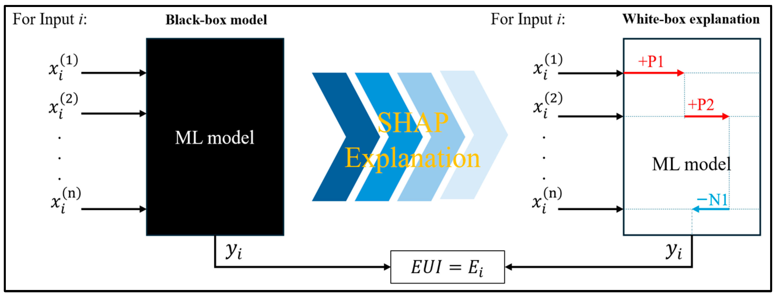
To address this issue, researchers have recently developed a new field of study named explainable artificial intelligence (XAI) to clarify the process of deriving models’ outputs by analysing the training and prediction procedure of the black-box models, including AI system and particularly ML models [7]. The XAI process aims to (1) improve ML models performance by analysing features used for training, (2) model stabilisation with investigating how changing feature values affects prediction results and facilitating designing flexible models which is stable to environments (3) to trust guarantees, particularly in the fields related to human safety [8].

Thus, various approaches have been proposed under the XAI framework, including model-specific interpretation techniques and model-agnostic methods that can be applied to any learning algorithm. Among these, feature attribution methods have gained significant attention for their ability to quantify the influence of each feature on the model’s prediction, which provides quantitative insights into model behaviour [9,10]. One of the most widely used feature attribution techniques is SHapley Additive exPlanations (SHAP), which is an effective tool for determining the effects of various input variables on model predictions.

Unlike traditional feature importance methods which provide only a global estimate for the influence of input variables on ML model outputs, SHAP provides detailed local explanations of the most influential parameters for each model predictions. This is particularly valuable when ML models are designed for building energy retrofit planning purposes.

The degree of influence of each feature on the output value can be calculated by the SHAP values which was first proposed by Lundberg and Lee as a unified measure of feature importance [8,11]. SHAP values offer both global and local interpretability by assigning an importance value to each feature for individual predictions. This technique can bridge between white-box and black-box modelling approaches by providing clear and quantified explanations for complex model outputs.

So, in this study, an ML model was developed to predict the annual energy consumption of residential buildings in the UK based on their characteristics, including building envelope and energy system parameters. In addition, the developed model was analysed using the SHAP framework to assess the local and global influence of different input features in the model. This interpretability analysis provides insights into optimal strategies for energy-efficiency retrofits and highlights potential areas for improvement in the developed model.

As mentioned earlier, there are various approaches for buildings’ energy modelling. In this context, Yu et al. [12] conducted a comprehensive review of the methodologies employed in white-box, black-box, and grey-box approaches for predicting building energy performance. They also analysed the sources of uncertainty associated with these prediction methods, considering factors such as occupant behaviour, building characteristics, and weather conditions. In particular, they concluded that with the growing availability of building energy consumption datasets and reduced dependency on detailed building parameter inputs, black-box modelling approaches such as ML, deep learning, and statistical analysis methods have emerged as an effective way for energy consumption prediction.

Research conducted by Ardabili et al. [13] focused on black-box approaches for energy consumption estimation and load prediction. The findings of this study ranked different approaches based on robustness, including ensemble methods, deep learning (DL) methods, linear regression methods, SVM-based methods, ANN methods, and hybrid approaches. Ensemble and deep learning methods were found to demonstrate the highest robustness, whereas SVM-based and linear regression models showed comparatively lower performance.

Similarly, Villano et al. [14] classified the most frequent ML and DL models used in this field and highlighted the advantages and limitations of each one. The reviewed ML models are including decision trees, random forest, naive Bayes, and SVM, and for DL approach they considered convolutional and recursive neural networks, long short-term memory, and gated recurrent units. More on ML models for buildings’ load forecast, Mohammed et al. [15] applied various models including XGBoost, random forest, classification and regression tree, and M5 tree model to predict heating load and cooling load of residential buildings. Results of this study highlighted a more accurate performance of XGBoost model in which R² values for predicting both heating load and cooling load recorded more than 0.97.

Recent studies have also highlighted the importance of uncertainty quantification in ML models, particularly for applications where predictions involve risk and long-term impacts. To address this, several approaches have been proposed that combine ML models with probabilistic or stochastic frameworks to estimate prediction uncertainty alongside ML model output. For instance, Mahajan et al. [16] proposed a Bayesian Neural Network (BNN) approach for probabilistic prediction of building energy demand to quantify prediction uncertainty alongside the raw predictions. This study compared BNN with LSTM-based models in terms of uncertainty quantification and prediction accuracy, which showed that BNN outperformed LSTM in uncertainty quantification as well as prediction accuracy. Furthermore, Xu et al. [17] provided a systematic review of uncertainty quantification methods in ML-based building energy modelling. They discussed sources of uncertainty and surveyed techniques used to assess and incorporate uncertainty in ML models for building energy prediction. While uncertainty quantification is beyond the scope of the present study, it represents an important direction for future work to further enhance the reliability of data-driven building energy models.

However, one of the key issues of the black-box modelling approach (particularly in the context of buildings’ energy modelling) is its lack of interpretability, meaning that the underlying relationships and contribution of each input variable trained in the model cannot be quantified. Although there are some metrics, such as “feature importance”, that calculate an index for different features to show their relative influence on the model’s output, they do not explain how individual features contribute to the prediction of each specific data point or case study, which limits their usefulness for detailed analysis in buildings’ energy modelling. In response, Lundberg and Lee [11] presented a unified framework for interpreting black-box models’ output called SHAP, which assigns each input feature an importance value for a particular prediction.

As a result, many studies have been conducted to utilise this framework for interpretation of data-driven models in different fields. Cui et al. [18] developed three different ML models to predict energy use intensity (EUI) in two common U.S. residential building types. In addition, they applied SHAP framework to analyse the impact of different features on ML models’ output and provided insights into its influence on EUI from global and local points of view. Based on the SHAP feature analysis on the most accurate models, the study suggested both general and building-specific strategies for improving energy efficiency in the case study buildings.

In a similar research, Zhou et al. [19] integrated ML models with SHAP analysis to explore how different energy-related factors influence carbon emissions in office buildings in China. Their approach involved training ML models to estimate building carbon emissions, photovoltaic (PV) carbon offsets, and overall net carbon emissions using more than twenty input variables. SHAP was then applied to interpret the model outputs at both global and local levels to provide a detailed analysis of features influence. The findings highlighted that the window-to-wall ratio and PV installation area play the most significant roles in determining carbon emissions and PV carbon offsets.

SHAP techniques have been utilised in various fields; one example is the research conducted by Cakiroglu et al. [20], which focused on improving the interpretability of ML models for wind turbine power predictions. This work estimated the power produced in a wind turbine using six different regression algorithms-based input features such as humidity, pressure, air density, and wind speed data. Utilising SHAP revealed that the wind speed is the most significant input feature that impact on the model predictions. Utilisation of SHAP is not limited to only engineering purposes in which it can be pointed to research conducted by Prending et al. [21] which utilised this method for interpreting black-box models developed for blood glucose prediction.

2. Materials and Methods

This chapter presents the overall research design adopted in the study which details the methods and techniques that were applied to achieve the research objectives, as it can observed in Figure 1. So, the selection and implementation of ML algorithms, the dataset selection and preprocessing, and the procedures followed for model training and evaluation will be discussed. Additionally, the methodology employed for interpreting model behaviour, particularly through SHAP-based explainability analysis, is described.

2.1. Dataset and Data Pre-Processing

The dataset utilised in this study is a synthetic, novel dataset generated through an automated parametric simulation workflow designed to represent the different types of residential buildings in the UK. The building archetypes were selected based on the categories defined in the Standard Assessment Procedure (SAP) for the UK housing stock [22], including detached, terraced, and mid-terraced layouts. For each archetype, a wide range of building characteristics was considered to capture different variations in the case study buildings. These parameters included envelope-related features such as wall, roof, and floor material, and insulation levels, along with energy system-related features such as heating system types (e.g., electric radiators, air-source heat pumps, and gas-fired combi boilers).

Furthermore, some detailed variables related to occupants’ consumption behaviour were assumed based on the UK National Calculation Methodology (NCM). This utilises typical values for detailed parameters in building energy simulations, such as occupancy pattern, interior lighting density, and internal heat gains. Analysing effect of these variables were either negligible on EUI or requires stochastic modelling approach which were beyond the context of this paper. Further details about the most important variables utilised in the dataset can be found in

Table 1. List of the most important considered features for dataset development.

General Details	Building Envelop	Energy System	NCM Pre-Defined
Location	External wall U-value	DHW system	Lighting power density
Building type	Floor U-Value	Heating system	Heat gains from equipment and occupants
Building layout	Roof U-value	Type of ventilation	Occupancy density and schedule
Adjacency	Glazing system
	infiltration

.

To generate the dataset, the different parameters were simulated using JEPlus–EnergyPlus co-simulation. As it was not feasible to simulate every possible combination of the input features (more than 100 million of simulation is required), Latin Hypercube Sampling (LHS) was employed to ensure an efficient and well-distributed exploration of the parameter space. This sampling strategy enabled balanced representation across the different classes within each feature category and also optimised the number of simulations required. The simulation process also incorporated a wide geographic range, with representative locations distributed from London in the south to Aberdeen in the north of the UK, which ensures that climatic variation was reflected in the dataset. In total, more than 8000 unique building samples were simulated, which provides a comprehensive set of energy performance outputs to be further utilised for model development.

Following the simulation stage, the dataset was organised, encoded, and scaled using different libraries in python. The available samples were also divided into training and testing subsets for the development and validation of the ML model.

2.2. Model Selection and Validation

For ML model selection, the XGBoost model is chosen since it has been widely used in the literature for building energy performance predictions, as well as its efficiency and ability to handle dataset with combination of categorical and numerical features [23,24,25]. XGBoost builds an ensemble of decision trees sequentially, where each new tree aims to correct the errors made by the previous ensemble by minimising a differentiable loss function. What makes XGBoost algorithm outstanding among other ML models is its ability to reduce overfitting by integration of a regularisation term into the model. In addition, its parallel and distributed computing system allows for faster training time, which leads to a more efficient modelling process [26].

Furthermore, there are many approaches for assessing the accuracy of a trained ML model. They can analyse an ML model from different aspects including difference between actual and predicted values, overfitting, outliers, etc. In this context, this paper has utilised k-fold cross validation with k = 5 for model performance assessment and investigating risk of overfitting and model bias. In this approach, the available dataset will be divided into k equally sized subsets, where the model will be iteratively trained on k-1 folds and assessed on the remaining fold to ensure that each subset was used once for validation.

In terms of performance metrics R² has been utilised to quantify the proportion of variance in the target variable explained by the model as it can be observed in Equation (1). Also, root mean square error (RMSE) and mean absolute error (MAE) have been utilised to highlight larger prediction error (outliers) and show the average of prediction error as shown in Equations (2) and (3).

$$R^2=1-{\displaystyle \frac{{\sum }_{i=1}^n{\left(y_i-{\widehat{y}}_i\right)}^2}{{\sum }_{i=1}^n{\left(y_i-{\overline{y}}_i\right)}^2}}$$

(1)

$$RMSE=\sqrt{{\displaystyle \frac{1}{n}} {\sum }_{i=1}^n{\left(y_i-{\widehat{y}}_i\right)}^2}$$

(2)

$$MAE={\displaystyle \frac{1}{n}} \sum _{i=1}^n\left|y_i-{\widehat{y}}_i\right|$$

(3)

where $n$ is the number of test cases, $y_i$ is the true value, and ${\widehat{y}}_i$ is the predicted value.

2.3. SHAP Methodology

SHAP is an XAI method based on the concept of Shapley values from game theory. In game theory, Shapley values provide a fair way to distribute total rewards among players based on their individual contributions. Figure 2 briefly shows how SHAP concept applies this idea to ML models which treats each feature as a “player” that contributes to the model’s prediction. On this context, the Shapley value ${\phi }_i$ for feature $i$ can be obtained from Equation (4) [19].

$${\phi }_i=\sum _{S\subseteq N}{\displaystyle \frac{\left|S\right|!\left(\left|N\right|-\left|S\right|-1\right)!}{\left|N\right|!}} \left[v\left(S\cup \left\{i\right\}\right)-v\left(s\right)\right]$$

(4)

where ${\phi }_i$ is the Shapley value that shows the effect of variable $i$ on a single prediction compared with the average of all predictions, $N$ is the set of all features, $S_i$ is the set of possible variable orderings, and $v\left(s\right)$ represents the optimum value that can be gained by coalition $S$. As stated before, in ML models, SHAP values are derived from the concept of Shapley values, which rely on conditional expectations to simplify how each input feature contributes to the model’s predictions [8].

Since calculating the exact SHAP values requires a lot of computation resources, the SHAP framework offers different approximation methods specific to each model type. For example, Kernel SHAP can be applied to any ML model, Deep SHAP is designed for deep learning models, and Tree SHAP is used for tree-based models. In Tree SHAP, the value of the final node in the tree represents the conditional expected value [27]. Since this study utilises XGBoost algorithm for ML model development, Tree SHAP has been applied for model interpretation.

3. Results

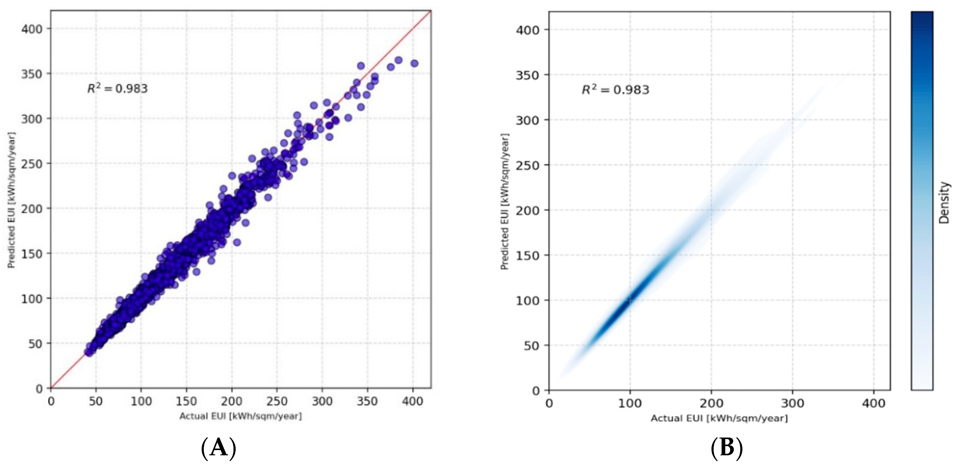
This section describes the accuracy of the developed ML model for predicting annual EUI and how this black-box model can be interpreted using SHAP method. First of all, Figure 3 shows predictive performance of the XGBoost model for more than 1500 test cases with scatter and kernel density estimation (KDE) plots. High coefficient of determination (R² obtained more than 0.98) shows the predicted EUI values closely tracking the actual values, which confirms the model’s high accuracy.

In particular, the scatter plot (A) shows that data points are concentrated around the diagonal line, which indicates the model consistently captures energy use behaviour across all building types. While high accuracy between actual and predicted values is observed over most of the EUI range, a slight increase in dispersion can be found for test cases with very high EUI values (which are relatively rare in practice) where the predicted values tend to deviate from the actual values, as it can be observed in the scatter plot. Finally, the KDE plot (B) also shows the highest concentration of test cases are around 100–120 kwh/m².year.

Also,

Table 2. Accuracy of developed ML model across 5 training and test folds.

	Fold-1	Fold-2	Fold-3	Fold-4	Fold-5
R2	0.981	0.984	0.984	0.986	0.985
RMSE	6.91	7.14	6.86	6.51	6.93
MAE	4.97	4.96	4.84	4.67	4.95

shows the model performance results summary of the developed ML model across five folds for predicting EUI using RMSE, MAE, and R² metrics. The consistent results across folds particularly indicate limited sensitivity to the training data and no sign of overfitting.

Moreover, as the research focuses on the interpretability of data-driven models, four case study buildings were selected; they represent a diverse range of typical residential building features summarised in

Table 3. Summary of the characteristics of the test case study buildings.

Case	Location	Building Type	Building Layout	Infiltration (ACH)	Heating Setpoint	Glazing U-Value	Floor U-Value	Roof U-Value	External Wall U-Value	Heating System	DHW System
A	Glasgow	Flat	End-terraced	1	23	3.0	2.02	0.558	0.212	Electric radiator	instantaneous
B	Norwich	Flat	Enclosed mid-terraced	0.4	22	2.5	0.25	0.667	0.251	ASHP	ASHP
C	London	Maisonette	Enclosed mid-terraced	1.2	18	1.0	1.005	1.097	0.677	Gas boiler	Gas boiler
D	Birmingham	House	Semi-detached	0.7	23	2.0	1.005	1.452	0.251	Electric radiator	instantaneous

. The test cases differ in location, layout, envelop, heating system, etc., which allows the behaviour of the ML model to be interpreted across a diverse spectrum of the UK residential buildings.

Case A is a flat in Glasgow with an end-terraced layout, heated with electric radiators, relatively high infiltration (1 ACH), a high heating setpoint of 23 °C, and relatively poor glazing and floor U-values. Case B is a flat in Norwich with a more sheltered enclosed mid-terraced layout, a lower infiltration rate of 0.4 ACH, and improved envelope performance compared to Case A, while being equipped with an air-source heat pump system. Case C is a maisonette in London with the highest infiltration (1.2 ACH) among the four cases but with significantly better glazing U-values, a combi gas boiler, and a lower heating setpoint of 18 °C. Case D, located in Birmingham, represents a semi-detached house with electric radiators and water instantaneous for DHW system. Across all cases, the predicted EUI is compared against the model-wide mean EUI of approximately 132 kWh/m².year, which forms the baseline from which SHAP values quantify positive or negative deviations.

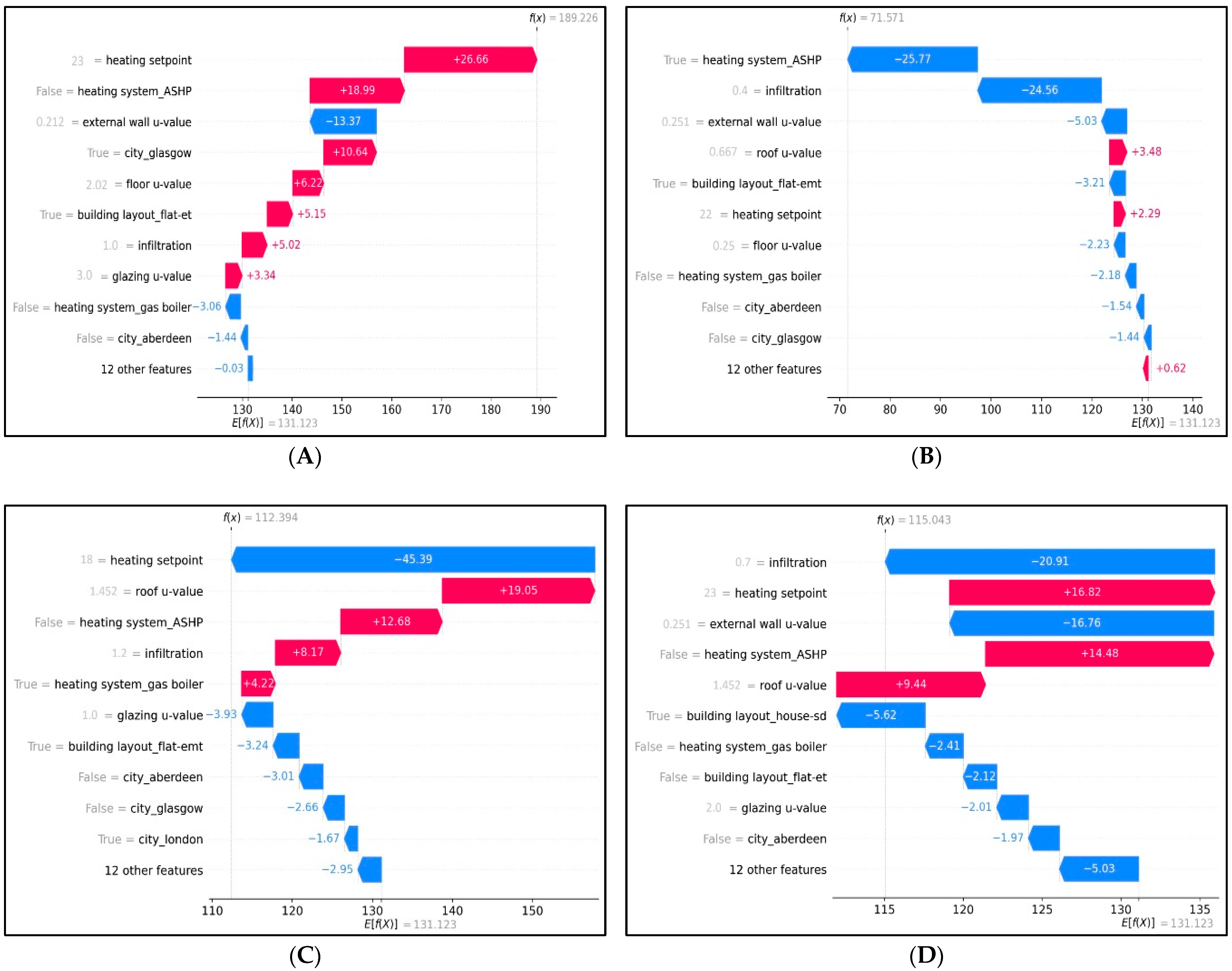
The SHAP waterfall plots in Figure 4A–D illustrate how the model reaches at the final EUI prediction for each case by decomposing the output into additive contributions from individual features. In Figure 4A, corresponding to Case A in Table 3, the predicted EUI is substantially higher than the dataset average, reaching approximately 189 kWh/m².year. The plot shows that the heating setpoint of 23 °C is the dominant contributor to this increase, adding more than 26 kWh/m².year to the baseline. The high glazing and floor U-values indicate significant thermal losses that also push the prediction upward. Glasgow’s climatic conditions also add a positive contribution, which is in line with the colder weather and higher heating demand typical of the region. On the other hand, some features, such as the low external wall U-value, produce negative contributions to shift predicted EUI towards lower values. As a result, Case A shows the highest EUI among the analysed buildings, primarily driven by high setpoint temperature, inefficient heating technology (compared to ASHP), and weak envelope components.

Figure 4B, associated with Case B in Table 3, shows a significantly lower predicted EUI of around 71 kWh/m².year in the case study, mainly due to utilising ASHP for heating and DHW system and lower infiltration rate (0.4 ACH) based on SHAP interpretation framework. High insulation level in external wall as well as enclosed layout of the building also contribute to the high energy-efficiency of this test case.

Furthermore, in Figure 4C, corresponding to Case C in Table 3, the model predicts an EUI of approximately 112 kWh/m².year. The SHAP waterfall breakdown shows that the low heating setpoint of 18 °C is the largest contributor which decreases the EUI prediction by over 45 kWh/m².year, which aligns with the significant impact that thermostat setpoint has on heating demand. The enclosed layout of the building and the low glazing U-value also reduce energy use. However, other factors, particularly the high infiltration rate of 1.2 ACH, the roof U-value, and utilising gas boiler instead of ASHP have dragged the EUI curve toward higher amounts. London’s warmer climate provides a slight downward adjustment, but the SHAP plot makes it evident that the interplay between a low thermostat setting and a relatively leaky envelope results in Case C falling near but below the mean EUI. The model effectively interprets this case as one where behavioural parameters (setpoint temperature) compensate for some of the deficiencies in the envelope and infiltration.

Finally, Figure 4D presents the SHAP explanation for Case D in Table 3, a semi-detached house in Birmingham with a predicted EUI of approximately 115 kWh/m².year. This prediction lies close to the dataset average, and the SHAP contributions are more balanced here than in the previous cases. The heating system and the heating setpoint of 23 °C again exerts a noticeable positive contribution. The roof U-value, at 1.452 W/m²K, is the highest among the four cases and therefore also adds significantly to energy use. On the other hand, the low external wall U-value and the building layout reduced the EUI to below the average.

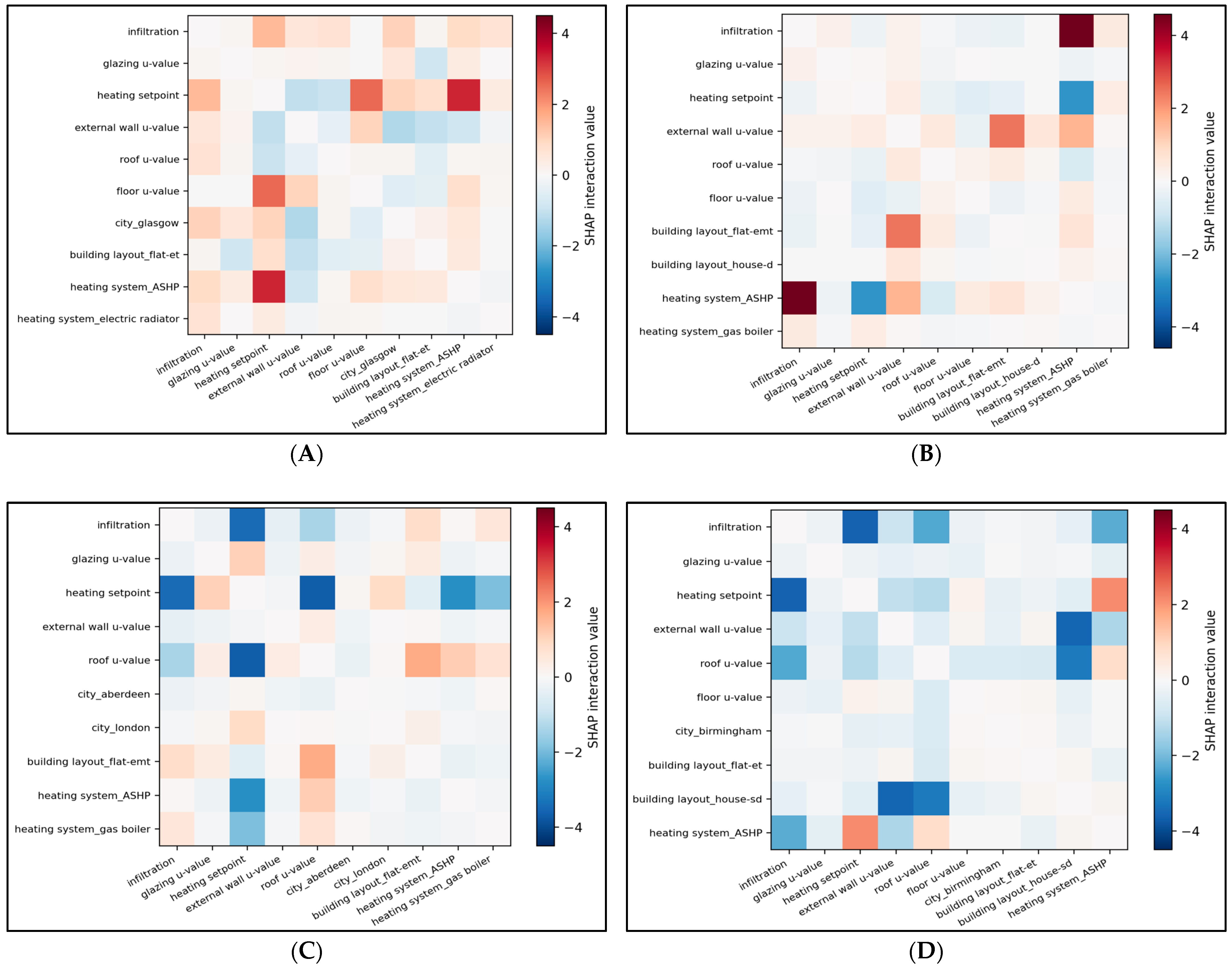
While SHAP waterfall plots provide clear local explanations for the model EUI output, they implicitly assume that features act independently. However, in building energy systems, many input variables are physically and operationally interdependent, such as infiltration rate and envelope insulation level, or heating system and location. To address this limitation and to avoid potentially misleading interpretations based on only waterfall plots, SHAP interaction values were further explored in Figure 5. SHAP interaction values quantify pairwise feature interactions for individual predictions; therefore, they facilitate local insights into how combinations of different building characteristics influence the predicted EUI. This capability is particularly valuable in residential retrofit planning, where energy performance outcomes often result from the interaction between envelope, system, and operational parameters rather than from single factors.

As it can observed in Figure 5, the local SHAP interaction plots presented for the selected case study buildings demonstrate that the developed ML model is able to quantify non-linear and co-dependant relationships between key variables, such as the interaction between infiltration and building envelop, or between heating system type and heating setpoint. These interactions help explain why similar changes in a single feature may result in different EUI outcomes across buildings with different characteristics. At the same time, it should be noted that SHAP interaction values remain limited to pairwise effects and do not fully resolve higher order dependencies among multiple correlated features.

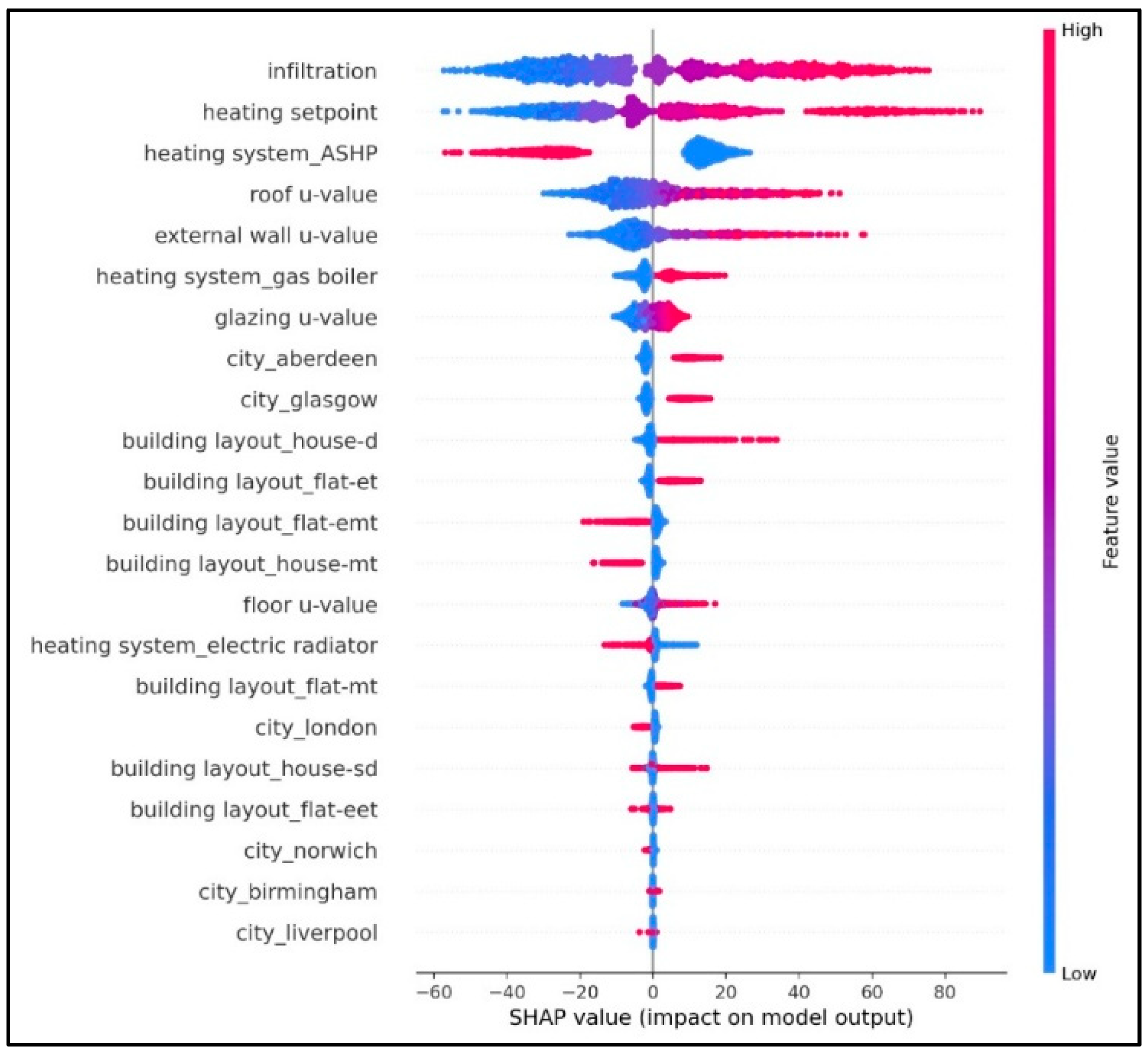
A SHAP summary plot is also shown in Figure 6 to illustrate the overall influence of each input feature on the model output by aggregating their contributions across the entire dataset. In this figure, features are ordered by their mean absolute SHAP values which enable the identification of the most influential predictors of EUI. The plot shows that infiltration rate, heating setpoint, and heating system type (particularly ASHP and gas boiler) impose the largest impact on the predicted EUI. Higher infiltration rates and higher setpoints consistently shift the predictions upward, whereas the presence of ASHP systems is strongly associated with reductions in EUI. Envelope-related features such as roof, external wall, glazing, and floor U-values also demonstrate significant contributions, with higher U-values generally pushing EUI upward due to increased heat losses. Location and building layout variables showed smaller yet non-negligible effects, which reflects regional climatic variations and differences in exposed surface area. Overall, the summary plot provides a global interpretability view which completes the case-specific waterfall plots by revealing how each feature drives the model’s predictions across the entire dataset.

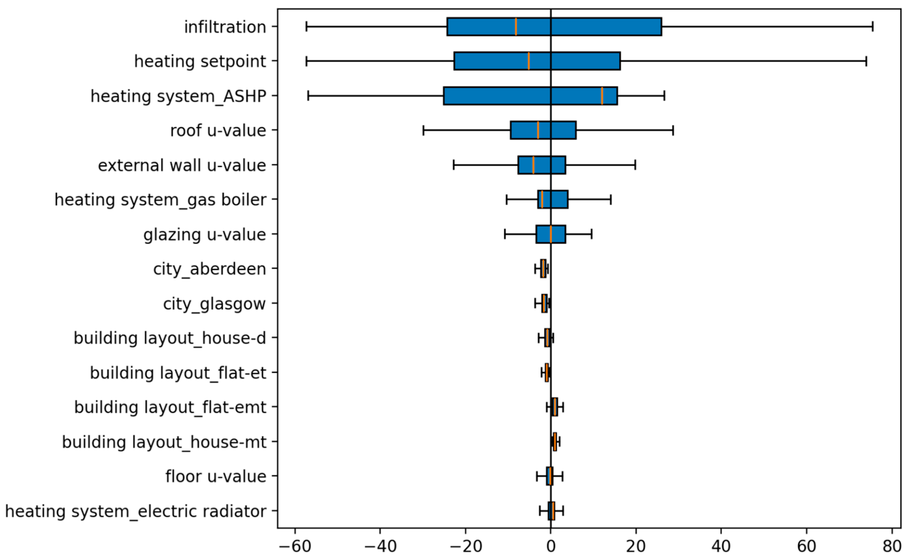
Similarly, the SHAP box plot is shown in Figure 7 to illustrate the statistical variance of SHAP values for the most influential features. Features such as infiltration rate, heating setpoint, and heating system type show both high median values and large variance which shows their impact on EUI differs substantially between case study buildings (data points). In contrast, envelope-related features such as glazing and wall U-values show smaller variance which represent generally lower contribution to EUI.

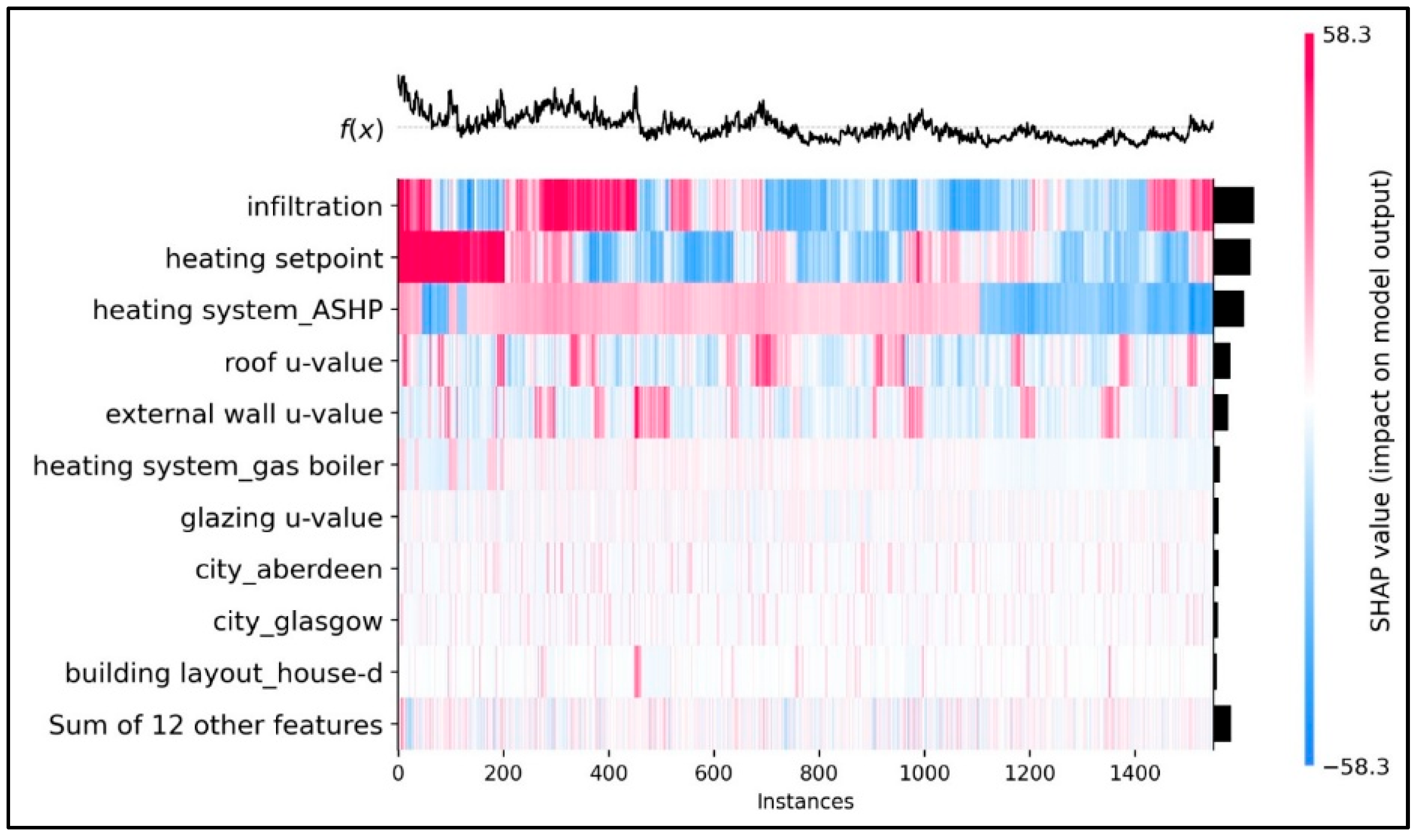
Finally, the SHAP heatmap plot in Figure 8 illustrates how the most influential input features affect the model output across 1500 test cases. In this figure, red colours represent positive contributions while blue colours represent negative contributions which indicates that the feature acts to reduce the EUI. Brighter shades of red or blue reflect stronger impacts, up to approximately ±58 kWh/m².year. Conversely, lighter or faded colours denote weaker influences on the model’s prediction. It can be observed that infiltration and heating setpoint show the strongest and most consistent effects across the test cases, as bright red and blue bars spanning in numerous samples.

In contrast, although other features such as the glazing U-value still contribute meaningfully to the model output, yet the relatively light shades of red and blue associated with them indicate that their influence typically remains within a narrower range, often around ±10 kWh/m².year. The heatmap effectively reveals not only the magnitude of each feature’s contribution but also the heterogeneity of these effects across different case study buildings.

All in all, the global representation of SHAP results in Figure 8 may indicate that retrofit strategies prioritising air-tightness improvements and heating system upgrades may achieve more substantial EUI reductions than minor changes to envelope U-values across a wide range of cases in this study.

4. Discussion

The results of this study showed that the developed XGBoost ML model provides highly accurate predictions of buildings EUI with an R² value exceeding 0.98, which highlights its robustness for large-scale energy performance assessment. This aligns with previous findings by Cui et al. [18], Mohammed et al. [15], and Osei-Owusu et al. [28], who also identified XGBoost as one of the most accurate models for predicting different types of buildings’ energy load. It should also be noted that the higher accuracy achieved in this study, compared to the results reported by Seraj et al. [1], who trained their model using the UK EPC dataset and obtained an R² value of around 0.82, reflects the greater consistency and reliability of the novel dataset developed here. Unlike the EPC dataset, which has been shown in several reports [4] and studies [29] to contain inconsistencies across different records and case studies, the synthetic dataset used in this research was generated under controlled conditions to ensure the accuracy and uniformity of data points used for ML model training.

Among different XAI interpretability methods, SHAP and LIME are two of the most widely used techniques for explaining black-box machine learning models. LIME provides local explanations by fitting a locally weighted linear surrogate model around an individual prediction to approximate the behaviour of the main model. On the other hand, SHAP provides both local and global interpretability within a single framework and is able to detect non-linear associations in the used model. In addition, an analysis of public GitHub repositories shows that SHAP has become the preferred XAI method among developers in recent years (utilised almost twice as much as LIME) [7].

So, the study showed that how the application of the SHAP framework enhances the interpretability of the developed model by quantifying the contribution of each input feature to the predicted EUI. The SHAP summary and heatmaps plots illustrated that infiltration rate, heating setpoint, and heating system type were the most influential parameters across different case studies’ EUI. These findings are consistent with the results reported by Cui et al. [18] and Zhou et al. [19], who observed similar dominant influences of operational parameters and heating systems on building energy consumption and carbon emissions.

From an interpretability point of view, SHAP analysis bridges the gap between traditional physics-based models and data-driven “black-box” approaches. While white-box simulations model energy systems through thermodynamic equations, they are computationally complex and unsuitable for large-scale applications. On the other hand, black-box models are efficient but vague. So, SHAP provides feature-level explanations of predictions to enable decision-makers understand black-box models’ prediction pattern. This interpretability is particularly relevant for retrofit planning, where identifying the most impactful parameters, such as infiltration or envelope insulation, can directly impact on cost-effective retrofit strategies.

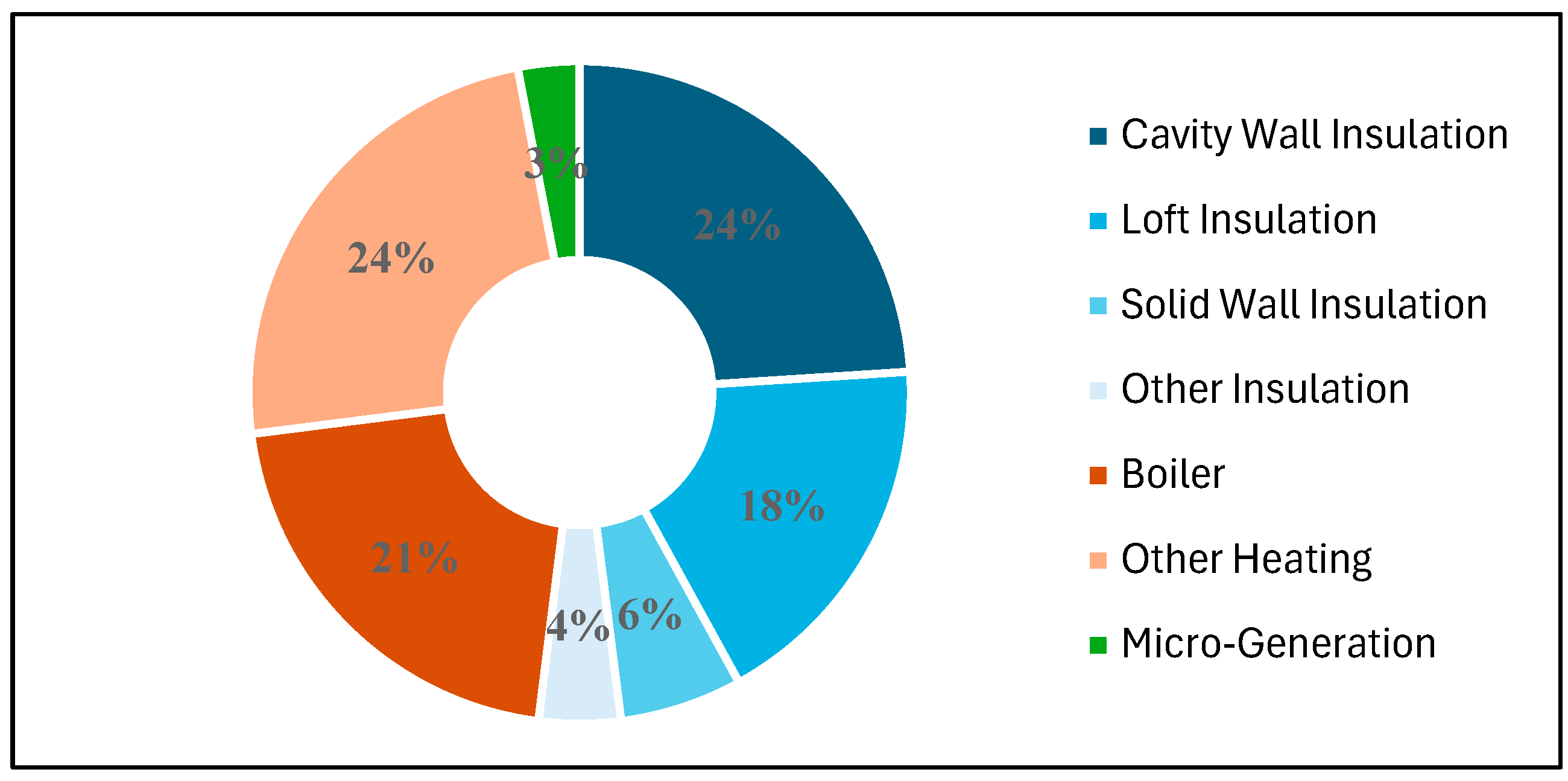
A practical example of how SHAP-based interpretability can support large-scale retrofit planning can be observed in an ongoing UK retrofit programme, Energy Company Obligation (ECO) scheme, which requires major energy suppliers to fund energy efficiency improvements in residential buildings. By the end of September 2025, approximately 4.4 million retrofit measures had been installed across 2.6 million households under this programme. As shown in Figure 9, the majority of these retrofits have focused on building envelope upgrades, with more than 52% of installed measures related to insulation improvements [30].

While insulation upgrades are one of the most important retrofit strategies, the SHAP analysis conducted in this study across more than 1500 test cases with diverse building characteristics and locations (Figure 8) suggests that, in many cases, improving building airtightness may offer comparable or even greater reductions in EUI. Interventions such as identifying thermal bridges, sealing unintended air leakage paths, and improving construction detailing can often be implemented at lower cost and with less disruption than deep envelope insulation retrofits. However, it should be noted that much more consideration should be taken into account in large-scale projects, but it was a brief example of how such models can contribute to large-scale energy retrofit planning.

Despite the model’s strong performance, several limitations should be noted. First, the dataset was synthetically generated and may not capture real-world variability such as occupant behaviour dynamics, maintenance quality, or system degradation. Future research could integrate measured energy data from buildings to validate and calibrate model predictions. Second, although SHAP effectively explained feature contributions, its computational cost increases with larger and more complex datasets. Developing more efficient approximation methods or combining SHAP with surrogate modelling could enhance scalability of the developed AI model.

5. Conclusions

This research aimed to address one of the key challenges in applying data-driven models for building energy performance prediction: the interpretability of black-box algorithms. To investigate this issue, a synthetic dataset was generated using an automated energy simulation process. This process generated over 8000 case-study buildings with a wide range of characteristics, such as different locations, building envelopes, and heating systems. This dataset was then used to train an XGBoost model, which was selected due to its efficiency and its capability to handle both numerical and categorical features. The trained model achieved an R² value of 0.982, which indicates strong predictive performance.

After developing the predictive model, a recently developed XAI method based on game theory, known as SHAP, was applied to interpret the model’s outputs. SHAP values were calculated to quantify the local and global contribution of each input feature to EUI predictions. Several SHAP-based visualisation tools, including summary plots, heatmaps, and waterfall plots, were utilised to analyse these effects.

The model interpretation results showed that infiltration, heating system type, and heating setpoint were the most influential features across the test cases, where their effect was observed more than 50–60 Kwh/m².year in some cases. In comparison, envelope-related features such as roof, wall, floor, and glazing U-values had smaller effects, usually within 10 to 20 kWh/m².year. The SHAP results suggest that building operation features can have a greater influence on EUI than minor changes in envelope U-value.

From a practical point of view, these findings suggest that retrofit strategies which focus on airtightness improvements, heating system upgrades, and heating control settings such as thermostat setpoints may result in greater energy savings than improving envelope U-value. The work also highlights the potential of interpretable ML models not only to predict energy performance but also to support retrofit planning by identifying case study specific drivers of energy consumption, rather than relying on generic assumptions or average trends.