Spatial and Temporal Unevenness in the Operation of Urban Public Transport and Parking Spaces

Abstract

This article examines the spatial and temporal unevenness of the transport complex operation in a large city with a population of about 0.9 million people and without off-street transport. The patterns of changes in the number of passengers transported in the city are described by a harmonic model, and seasonal unevenness with different numbers of peak values is noted. All routes can be divided into three groups based on the trend in passenger volume. The largest number of routes exhibited a downward trend in passenger volume. A downward trend in passenger volume is observed in the total number of passengers on all routes, despite an increase in the city’s population. Parking occupancy rates also show seasonal fluctuations. A downward trend in paid parking occupancy rates is emerging in the city’s central administrative and business district. The results of the study are relevant for choosing methods for managing the transport behavior model. Analysis of uneven passenger numbers on individual routes is necessary for improving the route network and determining the optimal number and passenger capacity of buses. Analyzing uneven occupancy rates in paid parking lots allows for the development of differentiated rates. The methods used in this article can be integrated into a city’s digital twin to improve forecasting accuracy.

1. Introduction

Urbanization is currently actively underway worldwide. Increasing urban density creates new challenges in ensuring sustainable citizen mobility [1]. The author of the paper [2] summarized 19 approaches to ensuring sustainable mobility. Many of these approaches reflect the need to reduce the use of private cars, including by ensuring the availability of public transportation and by influencing economic impacts through charges for the use of road infrastructure (parking, entry into the city center). Forecasting transport demand over time and space is essential to determining the need for new transport infrastructure. Macroscopic models that consider urban development scenarios (options) are used to forecast transport demand [3]. The proportion of city residents’ travel by means of transportation and modes plays a crucial role in developing these scenarios. To determine the share of travel by mode of transport in the future, it is necessary to forecast changes in the number of travels, i.e., to establish existing patterns and trends in their change. The level of development of public transport, road network, spatial settlement, and location of economic facilities significantly influence the choice of mode of travel by individual or public transport, i.e., influences the model of transport behavior [4,5,6].

Research in [7] shows that the pattern of transport behavior and the choice of travel mode exhibit spatial unevenness and depend on the location of the city district relative to the central part. The share of travel by public transport decreases with distance from the city center. For districts with the same distance from the center, the share of travel by public transport may differ due to different levels of public transport development. Notably, the level of public transport development is generally lower in newer districts of the city. This is due to the strategy for transport infrastructure development, and in the example under consideration, the city uses a compensatory (reactive) strategy, i.e., new routes and rolling stock are introduced into the transport system as demand arises from the residents. Given the gradual commissioning and occupancy of residential properties and the long period of approval and creation of new elements of the transport system, temporal unevenness is formed.

With the introduction of monitoring systems in the 1970s and 1980s, the use of time series to analyze traffic flow characteristics became widespread. Regression analysis was used to study peak-hour traffic flow rate and lane congestion [8]. Predicting the operating parameters of transport systems is complicated by complex dynamic interactions between spatial and temporal characteristics. This also impacts prediction accuracy [9]. One of the main problems encountered with existing approaches is the loss of valuable information when integrating spatial and temporal system parameters.

Spatial development analysis is conducted for both urban and regional transportation systems. In [10], the PageRank node centrality metric is used to quantitatively assess the importance of integration of individual nodes (e.g., stations, stops, and transport hubs) into the overall structure of a multimodal rail-road network (MRRN). The PageRank node centrality metric characterizes the importance of a node in terms of the structural connectivity of the entire network, taking into account not only the number of connections but also the influence of neighboring nodes. A high PageRank value for a node means that it is well connected to other important nodes, while a low PageRank value indicates that the area is peripheral and weakly connected to the main network.

An explosive growth and a transition to a new qualitative level in the study of sustainable mobility occurred with the digitalization of the economy, the implementation of the “Smart City” concept with the development of wireless data transmission technologies, and the IoT. The use of neural networks and machine learning methods made it possible to analyze the parameters of the urban transport system in real time and generate short-term forecasts of changes in the system state for 40–60 min [11,12]. Machine learning methods, deep learning models, and ANN are actively used in the study of population mobility and its structure [13], taking into account various modes of transport and travel. The accumulation of information and the formation of databases allow for the transition to long-term planning of the transport system. In [14], an ANN is used to predict the number of taxi trips and takes into account holidays, air temperature, and travel speed.

In recent years, all European countries have seen a decline in the share of buses and trains in domestic passenger transport [15]. Time series reflecting the number of passengers transported by public transport for the period 2020–2025 show a significant decline during the pandemic in 2020 [16,17,18]. The most significant declines were observed in Hungary, Poland, and Spain, and the smallest in Sweden.

The authors of [19] examined various models for predicting passenger traffic over time using machine learning. Based on statistical data, they found that routes have different characteristics and differ in criteria such as standard deviation, the presence or absence of seasonality, and long-term trends. All studied public transportation routes were grouped by several criteria, such as bus demand and occupancy. The article notes that predicting accuracy is important both for ensuring the quality of passenger service and for maximizing revenue for the transport company.

Machine learning methods and k-means clustering are used to study the factors influencing urban residents’ choice of public transportation. The authors of [20] note that travel time and punctuality are the most criticized aspects of public transportation. Cost is also a significant factor.

A popular measure to increase the attractiveness of public transportation in cities is the creation of bus rapid transit (BRT). Designing new BRT lines requires an analysis of passenger flow and prediction trends [21]. In their spatial analysis, the authors note that low population density reduces the efficiency of public transportation, and travel distance also influences the attractiveness of this mode of transport. Creating dedicated lanes for shuttle buses significantly impacts travel reliability (schedule adherence), which, over time, leads to an increase in passenger flow on these routes [22]. Therefore, when studying trends in passenger flow, it is advisable to consider infrastructure changes in the road network along which public transportation routes operate.

The relationship between changes in public transport system operating parameters in space and time is demonstrated in [23]. Public transport routes differ in the rate at which passenger traffic volumes recover on public transport when the route network for individual routes changes, and these trends can be both upward and downward. The authors attribute this primarily to the spatial characteristics of the routes and the city districts (based on the income level of residents) through which the public transport route passes. The authors of [24] examine the optimization of tram routes in Poland. The evaluation criteria include route parameters such as length, connections to districts, and rolling stock performance parameters such as speed, planned and actual travel times, and delays. To decide on route optimization, it is necessary to assess passenger demand and the dynamics of passenger traffic over several years, taking into account possible future trends.

When predicting public transport volumes, it is necessary to consider the development of new transport systems, such as driverless and autonomous vehicles. The introduction of new transport systems into the transport supply model could lead to significant adjustments to established trends in the operation of existing modes of transport [25]. The authors also note the problem of poor service levels by bus routes for city residents in suburban areas. As a result, these areas have become car-centric due to an insufficient mobility offer. In the absence of dedicated public transport lanes, shuttle buses travel along the street and road network in the general flow. Bus performance depends on the parameters of the overall flow. Instantaneous megatraffic caused by the uneven spatial and temporal distribution of transport demand is a significant problem in metropolitan city management [26]. To mitigate this problem, this article examines algorithms for generating dynamic public transport routes (with a request for a travel start time and a variable route).

The need for a thorough analysis of public transport development measures is determined not only by economic and infrastructural criteria, but also by environmental ones, which together shape sustainable mobility. The authors of [27] show that the growth dynamics of harmful emissions from public transport over time are significantly lower than those from private cars and taxis. Therefore, cities are actively developing public transport and restricting the use of private cars.

To improve the efficiency of traffic management in cities, intelligent transportation systems are being implemented. For intelligent transportation systems, accurately forecasting travel demand in cities is a challenging task due to complex spatiotemporal dependencies, its dynamic nature, and uneven distribution. Existing forecasting methods based on static spatial dependencies do not take into account the impact of the diversity of dynamic demand patterns and/or uneven distribution. The authors of [28] propose a travel demand forecasting model for cities based on a hybrid dynamic graph convolutional network (HDGCN). Simulation is conducted in three stages. First, the dynamic nature of travel demand and the time series are taken into account. Next, spatial features are determined from the dynamic and static graphs, respectively. In the third stage, the spatial features are studied along with the temporal features of the system.

The development of agglomerations and urbanization leads to an increase in the number of trips, average travel distance, and travel time [29]. There are cases where the number of residents in cities is not calculated, and even with a constant number of trips, the load on the road network increases due to the increase in travel distance.

A new approach to macromodeling of transportation systems using graph neural networks (GNNs) is proposed in [30]. The authors develop a surrogate model capable of replacing traditional, computationally expensive four-stage macromodels. Such a model is expected to provide high accuracy while significantly reducing the time required. The model is trained using transport macromodel data and is used to forecast correspondence matrices, transport and passenger flow parameters, taking into account demographic data, infrastructure, and baseline scenarios for transport demand and supply macromodels.

The development and application of a deep learning model for predicting the evolution of traffic jams across the entire urban transport network is described in [31]. Particular attention is paid to the model’s ability to predict not only the current but also the future state of traffic jams in a spatiotemporal context. Establishing patterns in the operation of the urban transport complex is necessary for strategic planning and the formation of a set of measures for the development of the city for a period of 10–20 years.

The aim of this study is to establish the spatial and temporal unevenness in the operation of the urban transport complex using the example of a large city without off-street transport with a population of up to 1 million people. Achieving this goal will improve the methodology for analyzing urban transportation system performance, taking into account seasonal cycles. This work aims to establish patterns of changes in the number of passengers carried on individual public transportation routes and the occupancy rate of paid parking lots in the city center. The significance of this research lies in improving the accuracy of forecasting urban transportation system performance parameters, taking into account emerging trends in public transportation and parking space. The following methods are used in the research: theoretical and hypothetical methods, a systems approach, field observations, mathematical modeling, correlation, and regression analysis.

2. Materials and Methods

2.1. Methods

Despite the steady growth in the use of personal mobility devices and bicycles, public transport and private cars remain the primary modes of medium- and long-distance travel. Therefore, this study examines the performance of these two subsystems of the urban transport system. Data on the operation of the transport system during the research were collected using currently existing monitoring systems and automated processing of data from detectors. Automation of the process and the use of existing monitoring systems are necessary for generating large amounts of initial data (big data), which allows for evaluating system parameters over a long period (day, month, year) without significant research effort.

When studying the spatial and temporal unevenness of transport system operating parameters, the transport system is treated as a “black box,” accounting for the boundaries of the system under consideration without examining the processes within it. All model variable values are quantitative indicators that vary widely.

Using actual data from transportation monitoring systems, two datasets were obtained to establish the temporal and spatial characteristics of system operation. The study was conducted in two stages, focusing on individual subsystems of the urban transportation system. The first stage examined the unevenness of transportation system operation over time over several years, using public transportation on selected, highly used routes as an example. The second stage examined the unevenness of paid parking occupancy in the city center over the course of a year. The choice of two subsystems (public transportation and paid parking) as the research subject was driven by their interdependent importance. Paid parking rates influence travel mode choice and, consequently, the number of passengers carried on public transportation. The opposite effect also occurs: as the attractiveness of public transportation increases, city residents partially abandon private transportation, and parking lot occupancy decreases.

The operating parameters of the urban transport system are determined by the activities of city residents. The number of city residents’ activities fluctuates throughout the year due to summer school and university holidays, vacation seasons for working citizens, public holidays, and the growing season for berries, vegetables, and fruits in private suburban gardens.

The research concept was as follows: due to the spatiotemporal unevenness of urban transport system operating parameters, improving its efficiency requires implementing adaptive process management within the transport system and a differentiated approach to determining optimal control actions. The study hypothesizes seasonal variations in public transport operating parameters and parking occupancy, as well as differences in time series parameters for different public transport routes.

2.2. Study of the Unevenness of Passenger Volume over Time

Unevenness in the number of trips on public transport is highly evident both spatially and temporally. However, managing the public transport system offers less variability in potential measures and a longer implementation period. With the exception of dynamic public transport routes with variable schedules and routes, operational changes to the vast majority of routes are impossible. Unlike the road and street network, the route network is less extensive and less spread out, and has a number of limitations and mandatory conditions. Changes to the route network and schedules require lengthy justification, calculations, approvals, and a study of the impact of decisions on a single route, taking into account the connections between routes, their duplication, and the number of buses on the route. Rapid changes are also limited and regulated by contractual relationships between the municipality and carriers.

Objective decisions must take into account the influence of transport demand and weather conditions on the system’s operating parameters. Therefore, the study of uneven public transport system operating parameters evaluates the number of passengers carried on a specific route and uses a five-year period with a one-month increment.

The observed dynamics of the number of passengers transported by public transport is characterized by a pronounced spatiotemporal heterogeneity. Let R = {r₁, r₂, …, r_N}—multiple public transport routes, T = {t₁, t₂, …, t_N}—analysis time interval (in months), and Y_r(t) ∈ N₀—number of passengers transported by urban public transport on the route r ∈ R at a time t ∈ T.

To assess the unevenness of passenger volume over time t for route r, the variation coefficient CV_r is applied and defined as follows:

CV_r = σ_Y(r)/μ_Y(r)

(1)

where σ_Y(r) is the standard deviation of the volume of public transport passenger traffic, and μ_Y(r) is the mathematical expectation of the number of passengers transported on routes.

To assess the unevenness of the number of passengers between individual routes r at time t, the variation coefficient is applied and is defined as follows:

CV_t = σ_Y(t)/μ_Y(t),

(2)

where σ_Y(t) is the standard deviation of the number of passengers transported on individual routes over time, and μ_Y(t) is the mathematical expectation of the number of passengers transported on individual routes over time, if Y(t) = {Yr₁(t), Yr₂(t), …, Yr_N(t)}

The variability of the values of the variation coefficient by route at a fixed point in time indicates a high spatial differentiation in the number of passengers transported.

In contrast to the street and road network, where operational regulation of flows is possible (traffic lights, reversible lanes, dynamic restrictions), the set of permissible control actions U_r for the route r in the public transport system is significantly limited:

$${\mathrm{U}}_{\mathrm{r}}\subseteq \{\Delta {\mathrm{f}}_{\mathrm{r}}, \Delta {\mathrm{L}}_{\mathrm{r}}, \Delta {\mathrm{\tau }}_{\mathrm{r}}\}$$

(3)

where U_r is the set of permissible control actions, Δf_r is the change in the movement frequency (interval τ_r = 1/f_r), ΔL_r is the change in the route way, and Δτ_r is the schedule shift.

At the same time, most routes do not support dynamic adaptation of ΔL_r(t) ≠ 0, and the set of actually realized effects is narrowed down to

$$U_r^{real}=\{\Delta f_r | \Delta f_r=const,\forall t\in \left[t_0,t_0+\Delta T_{\min }\right]\}$$

(4)

where ${\mathrm{U}}_{\mathrm{r}}^{\mathrm{real}}$ is the set of actually realized effects, t₀ is the point in time of the beginning of the implementation of adaptation measures, and ΔT_min is the minimum regulated period of schedule stability (usually ≥ 3–6 months).

Any change in the route or schedule of u ∈ U_r requires a decision-making procedure, formalized as follows:

$$\mathrm{u} \in {\mathrm{U}}_{\mathrm{r}}^{\mathrm{e}\mathrm{x}}\iff \Phi (\mathrm{u}, \mathrm{r}, {\mathrm{R}}_{\mathrm{conn}})\ge \Theta ,$$

(5)

where Φ(⋅) is the justification function, including calculations of loading, duplication with other R_conn ⊂ R routes, rolling stock requirements, socio-economic consequences, and Θ is the eligibility threshold set by the regulator.

In addition, the set of permissible management actions is limited by contractual obligations between the municipality and carriers:

$${\mathrm{U}}_{\mathrm{r}}^{\mathrm{d}}=\{\mathrm{u}\in {\mathrm{U}}_{\mathrm{r}} | \mathrm{C}\left(\mathrm{u}\right)\le {\mathrm{C}}_{\max }, \Delta {\mathrm{t}}_{\mathrm{real}}\left(\mathrm{u}\right)\ge \Delta {\mathrm{t}}_{\mathrm{d}}\},$$

(6)

where C(u) is the cost of Implementing Impact, C_max is the total capabilities (limitations) of the municipal budget for the implementation of management actions, Δt_real(u) is the minimum implementation period, and Δt_d is the contractually fixed period of stability.

To objectively assess the regularities of the system’s functioning, it is necessary to take into account the influence of exogenous factors: seasonality s(t) ∈ S and weather conditions w(t) ∈ W. In this case, the number of passengers transported by the urban public transport model can be represented as

Y_r(t) = f_r(s(t), w(t), ε_r(t)),

(7)

where ε_r(t) is a random component reflecting unpredictable perturbations, s(t) is a seasonal component reflecting seasonal fluctuations and cyclicity, and w(t) is a weather factor that reflects fluctuations due to changes in weather conditions.

To sustainably assess seasonal effects and minimize the impact of short-term anomalies, the study uses a five-year observation interval of T = 60 months with a step of Δt = 1 month. Despite the high spatiotemporal variability of demand {Y_r(t)}, the public transport control system has significant inertia and a low degree of freedom in the space of control actions U_r. This necessitates the following:

• Developing long-term adaptive strategies based on long-term trends;
• Creating flexible response mechanisms within the acceptable subset of U_r;
• Integrating forecasting models into planning processes.

Thus, the analysis was carried out on an aggregated monthly grid for 5 years, which ensures the statistical stability of the conclusions and makes it possible to formalize the limitations in the synthesis of management decisions in a rigid institutional environment. The functioning of the urban transport system is characterized by the temporal non-uniformity of the X(t) state parameters, and the use of the adaptive management strategy U_ad(t), based on the current state of the system and differentiated by spatiotemporal segments, significantly reduces the value of the efficiency functional J in comparison with the use of a static (non-adaptive) or unified strategy U_st(t) ≡ const or U_un(t) = f(t), which does not take into account the local features of routes or zones.

The number of passengers in the public transport system was calculated based on bus fare payment transactions on all routes along the studied routes over a period of 5 years. All public transport payment transactions are recorded in the automated fare collection system (AFCS) using a conductor’s mobile terminal for payment by bank card or cash. The primary dataset contains records of 254,411 million fare payment transactions, including date, route number, trip number, time, payment method, and the ID number of the public transport card or bank card. Considering that there are conductors on each bus for all routes, the percentage of passengers purchasing a ticket approaches 99.5%. Automation of the payment process and conductor control over payment ensures the reliability of the database. No additional data cleansing was required. The AFCS 3.0 software generates databases for individual days, months, and years for each route. The dataset on the number of passengers (dependent variable) contains data for 60 months (independent variable) on 48 public transport routes. The total dataset consisted of 2880 values.

To analyze and process data on the number of passengers transported, the Python 3.10 programming language and the following library versions were used: numpy 1.26.4, pandas 2.2.0, matplotlib 6.7.1, seaborn 0.13.2, statsmodels 0.14.4, scikit-learn 1.1.1. MS Excel was used to approximate harmonic models and evaluate their statistical characteristics.

The Dickey–Fuller test was used to test for non-stationarity in the time series. Harmonic analysis and the harmonic linearization method were used to determine the seasonal component of the time series. To classify and analyze the differences between routes based on the criterion of the number of passengers transported, routes were grouped into quantiles.

A quantile is a value that divides an ordered data sample into two parts such that a specified proportion of the data lies below this value, and the rest lies above it. In other words, a quantile indicates the boundary below which a certain percentage of observations lie. A quantile is a statistical measure that defines the value of q_a ∈ R, such that for a given level of α ∈ (0.1), the following condition is satisfied:

P(X ≤ q_α) ≥ α and P(X ≥ q_α) ≥ 1 − α,

(8)

where X is a random variable corresponding to the distribution of the number of passengers transported by urban public transport along the routes, and P is a probabilistic measure (in the case of sampling, an empirical distribution function).

In this study, quartiles were used to categorize routes by load level—quantiles of the order α = 0.25, 0.50, 0.75, designated as Q₁, Q₂, and Q₃, respectively. Thus, the set of all routes R was divided into four non-overlapping subsets based on the volume values x_i:

• “Very High Load”—routes in the upper quartile (75–100%), with the highest number of passengers transported by urban public transport, for which xi ∈ (Q₃, +∾), that is x_i > q^0.75;
• “High Load”—routes in the 50–75% quantile, for which x_i ∈ (Q₂, Q₃), that is q^0.5 < x_i ≤ q^0.75;
• “Medium Load”—routes with the passenger volume in the 25–50% range, for which x_i ∈ (Q₁, Q₂), that is q^0.25 < x_i ≤ q^0.5;
• “Low Load”—routes in the lower quartile (0–25%), having a minimal number of passengers transported by urban public transport, for which x_i ∈ (−∾, Q₁), that is, x_i ≤ q^0.25.

Below is a boxplot that visualizes the distribution of data by category and allows you to compare mean values, spread, and outliers (Figure 1).

2.3. Study of the Unevenness of Parking Space Operation over Time

To study the unevenness of demand for paid parking services for private cars, we selected the daily operating period from 8:00 AM to 6:00 PM, taking into account their weekday operating hours. The largest number of trips by private cars is made for work and educational purposes, so to account for the unevenness over 10 h of paid parking operation during the day, the study assessed parking occupancy at minimum intervals of one hour. Several indicators were used to assess the unevenness, including average parking time and changes in parking occupancy throughout the day.

The dataset on parking operations recorded the times a vehicle entered and exited a paid parking lot (dependent variable) throughout the day (independent variable), allowing for the generation of several calculated indicators. The entry and exit of vehicles to and from the parking lot were automatically recorded by opening and closing the barrier and using a specialized electronic card. Drivers received the electronic card from the terminal before opening the barrier upon entering the parking lot and presented it to the terminal to open the barrier upon exiting. Without the card, it was impossible to enter the parking lot, and all parking sessions were recorded in the database.

The object of the research was data on the daily operation of paid city parking lot No. 101 at the address: Tyumen, Pervomayskaya Street, 20, for the period from January 2023 to March 2025. The dataset contains records of 232,457 parking sessions, including the date, start time, end time, estimated duration of the parking session, payment method, and the parking card number. The provided data contained 254 missing values in the “Parking card number” column, as payment was made in cash. This did not affect the data quality; the missing values were replaced with the “No number” label. No further data cleansing was required.

The following Python 3.10 libraries were used for data analysis: numpy 1.25.2, pandas 2.0.3, scikit-learn 1.5.2; prophet 1.2.1, statsmodels 0.14.4 (SARIMAX, seasonal_decompose)—for time series analysis and forecasting; matplotlib 3.9.2, seaborn 0.13.2—for visualization. The stationarity analysis of the time series of daily parking usage (in minutes) is performed using the Dickey–Fuller test.

2.4. Research Hypothesis

The study hypothesizes that seasonal variation in the number of public transport passengers and parking sessions can be described by a harmonic model, with time series parameters differing across public transport routes.

The time series for the number of passengers carried, the number of parking sessions, and the occupancy rate of paid parking lots are described by the following equation:

$$Y_i=Y_0+{\displaystyle \sum _{k=1}^g{A}_{Yk}\cos (m(k{T}_i-T_{0k}))}$$

(9)

where Y₀ is the average value of Y per cycle, k is the harmonic number, g is the number of harmonics, A_Yk is the half-amplitude of the k-th harmonic oscillation, m is an interval between T_i and T_i+1 in degrees, and T_0k is the initial phase of the oscillation in degrees.

Harmonic models are well-known and are actively used in various fields, such as mathematics, physics, economics, and engineering. In this study, we propose using a harmonic model to assess the fluctuations of system parameters when studying changes in the number of passengers transported and parking lot occupancy by month. The article is devoted to the development of methods for studying changes in individual parameters of the state of public transport and parking space over time, taking into account the possible dependence on the spatial unevenness of the development of systems.

To test the hypothesis in accordance with the hypothetical method, it is necessary to confirm the adequacy of the proposed harmonic model and conduct experimental studies.

3. Results

3.1. Analysis of the Spatiotemporal Unevenness in the Operation of Public Transport Routes

Experimental studies were conducted using the observational method. Temporal unevenness of the volume of transportation (number of passengers transported) by urban public transport was assessed in three stages: assessment of stationarity, seasonal unevenness, and unevenness by year (trend). Uneven public transport volumes were assessed using harmonic time series analysis. This involves identifying trend, seasonal, and random components. The study focused on monthly passenger volume data for 48 city routes from 2018 to 2022. For ease of interpretation, all routes were classified by average monthly passenger volume over a five-year period. The classification was based on four quantiles.

Each box in the boxplot graph (Figure 1) shows the following characteristics for the number of passengers transported along public transport routes.

The lower boundary of the box is the first quartile (quantile of the order = 0.25: 25% of the values in the category lie below this boundary. In the “Very High” category, even 25% of routes carry more than 106,000 passengers per month.

The line inside the box is the median (quantile of the order = 0.50): half the values are above, and half are below. Thus, for the first category of routes with very high passenger traffic, the median corresponds to a value of 236,000 passengers per month, and for the fourth category, it does not exceed 4471 passengers per month.

The upper boundary of the box is the third quartile (quantile of the order = 0.75): 75% of the values are below this boundary. For the second category with high passenger traffic, 75% of the values are below 44,294 passengers per month. In the “Medium” and “Low” categories, the range of values is 8510–12,504 and 3336–5068 passengers, which indicates that these are fairly homogeneous groups. The whiskers (lines from the box) encompass values within 1.5× the interquartile range (IQR) from the edges of the box. For the very high-loaded routes category, the top line of the box is twice the third quartile and equals 600,000 passengers, meaning there are some routes in this category that carry more passengers than others. Points outside the whiskers are outliers: values that differ sharply from the others.

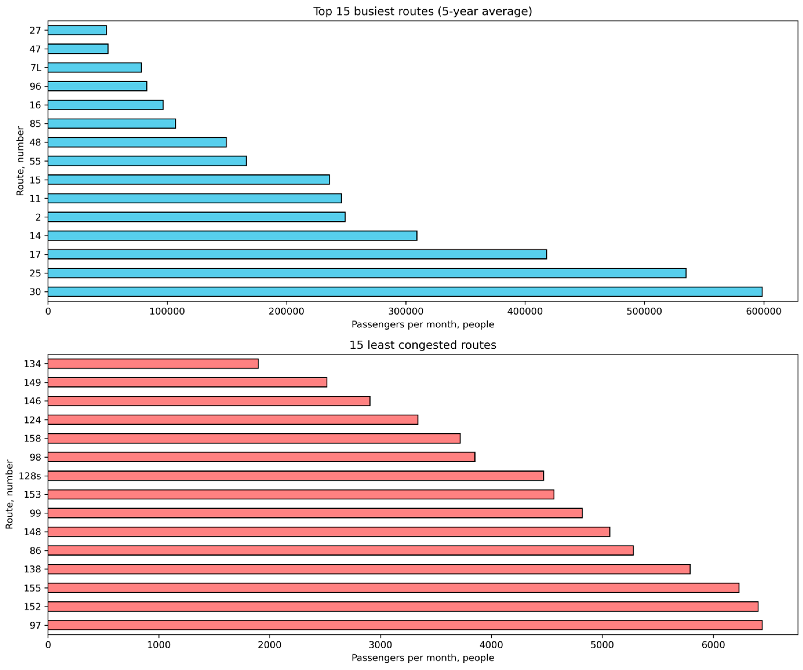
The horizontal bar chart (Figure 2) lists the 15 routes with the highest (top) and lowest (bottom) passenger volumes. The chart shows that route No. 30 carries the most passengers, averaging approximately 600,000 per month, while route No. 134 carries the least (2000).

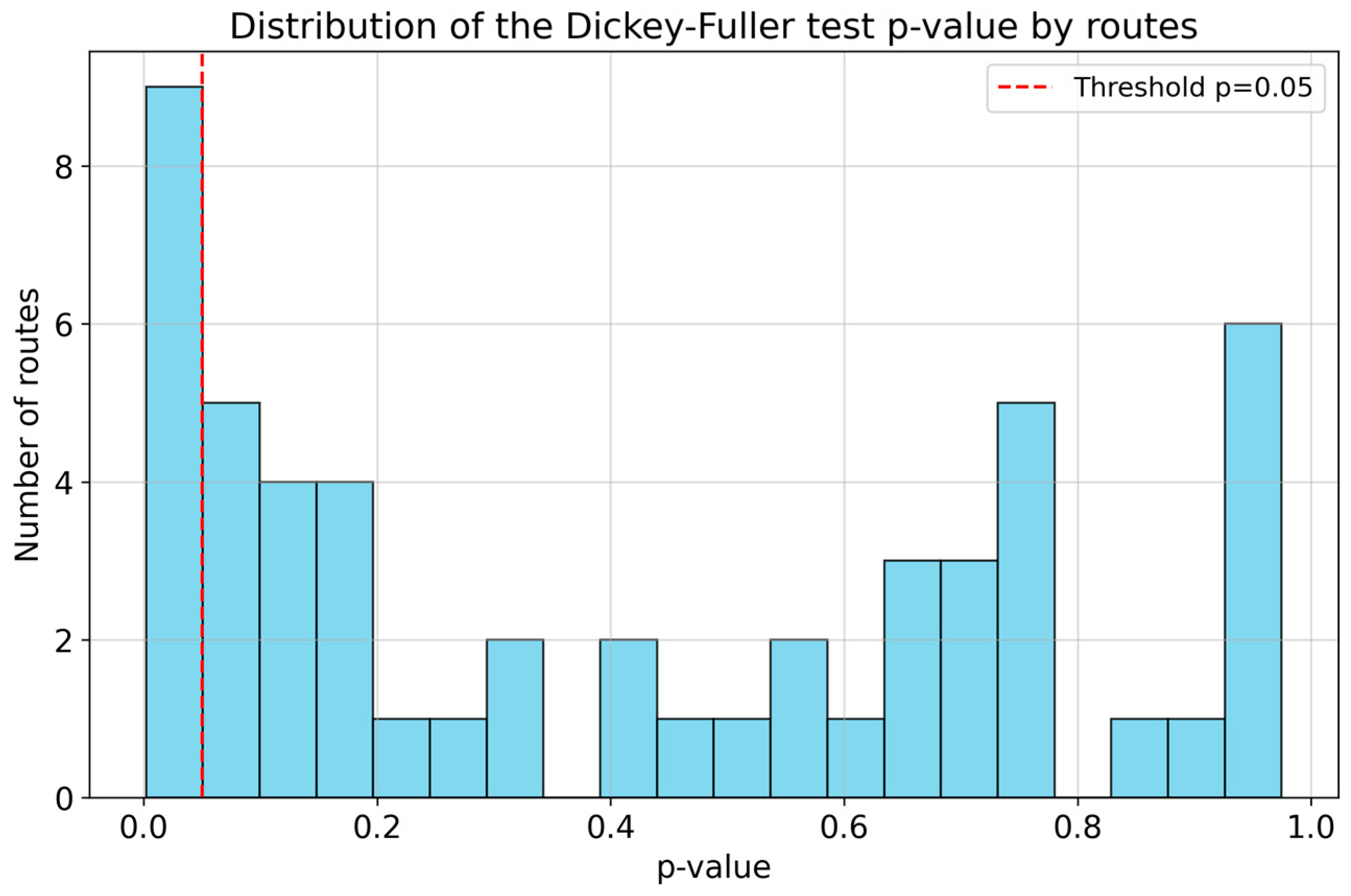
All routes were assessed for stationarity using the Dickey–Fuller (ADF) test. A time series is stationary if its mean does not change over time, its variance is constant, and there is no trend or seasonality (or these are eliminated). If the ADF test result yields a p-value of p < 0.05, the series is stationary (or has a unit root, but the hypothesis of non-stationarity is rejected). If p ≥ 0.05, the series is non-stationary—there is a trend, seasonality, or mean drift. As a result, the majority of routes are non-stationary, and the percentage of stationary routes is 17.3% (Figure 3).

Identifying seasonal fluctuations in a non-stationary time series of changes in the number of passengers carried by public transport will allow us to identify periods of peak and trough transport demand throughout the year. This will allow us to determine the optimal number for passenger capacity of buses operating on specific routes. During periods of declining passenger numbers, adjusting and reducing the number of bus trips can reduce system operating costs, while during periods of increased demand, creating comfortable conditions on buses can improve the quality of public transportation. All of this combined makes the urban public transportation system more adaptive to changing conditions and ensures sustainable mobility. Knowing the time series of passenger numbers allows us to refine the city’s transport macromodels and make them universal for the entire year when developing models based on data from a single season. This makes the models more relevant to real-world changing conditions.

Further analysis of passenger volume changes on various routes in Tyumen allowed us to identify three categories of routes: routes with an increasing traffic trend, routes with a decreasing trend, and routes with no trend change. To test the stability of the cluster distribution, the silhouette coefficient metric was used, a high value of which for a given number of clusters indicates the quality of clustering or the stability of the partitioning into clusters. For categorization, we used the difference between the average annual value and the standard deviation, as well as the R² coefficient of multiple determination and the standard error for the linear regression equation. If the average annual value changes between years were within the standard deviation, the trend change was considered insignificant.

All routes can be divided into 3 categories based on the trend in the number of passengers carried:

• With a decreasing trend (21 routes): 25, 30, 11, 14, 15, 17, 20, 27, 47, 48, 60, 86, 97, 98, 99, 119, 129, 135, 141, 149, 155;
• With an increasing trend (5 routes): 2, 18, 33, 100, 144;
• With no trend (constant average) (22 routes): 9, 10, 16, 32, 53, 55, 63, 85, 91, 96, 100 k, 121, 124, ‘128 s’, 134, 138, 146, 148, 152, 153, 156, 158.

All routes are not stationary throughout the year, meaning they exhibit cyclical patterns (temporal irregularities). Moreover, the cyclical patterns on individual routes can vary significantly depending on peak periods of the year. For example, some routes have cyclical peak traffic volumes during two peak periods: fall and spring (route 25), fall and winter (route 91), and a single peak period—spring only (route 18) or summer (route 97). The analysis of routes from different groups was conducted using two routes for each of the above-mentioned trend change categories. Within individual clusters, two routes were selected for which the indicator of the number of passengers transported is in the middle of the range of variation of values. For a more complete analysis of the temporal unevenness, considering the demand for the route among city residents, public transport routes from all groups with the highest, lowest (Figure 2), and average number of passengers transported per month were selected. The list of the analyzed routes is presented in

Table 1. Representative routes for three categories of routes with different trends in passenger traffic volumes.

Route Category	Route No.	Route Length, Travel Interval	Number of Peaks	Peak Periods
Increasing trend	2	Lr = 26.1 km, I = 15 min	2	fall and spring
	18	Lr = 13.3 km, I = 45 min	2	spring
Decreasing trend	30	Lr = 18 km, I = 5 min	2	spring and fall
	97	Lr = 28.7 km, I = 120 min	1	summer (suburban route)
Trend remains unchanged	91	Lr = 16.2 km, I = 110 min	2	fall and winter
	134	Lr = 22.4 km, I = 180 min	1	summer (suburban route)

. The values of the above-mentioned coefficients for the trend lines of the routes under consideration are presented in

Table 2. Parameters of the equation for the annual trend of change in the volume of passenger transportation.

Route No.	Changes in Transportation Volumes, %	R2 Value for the Linear Equation Approximating the Annual Trend	Mean Squared Error (MSE) Value
2	+26.9	0.43	0.43
18	+134.4	0.67	0.67
30	−29.2	0.60	0.60
97	−26.4	0.48	0.48
91	-	0.02	0.02
134	-	0.002	0.002

.

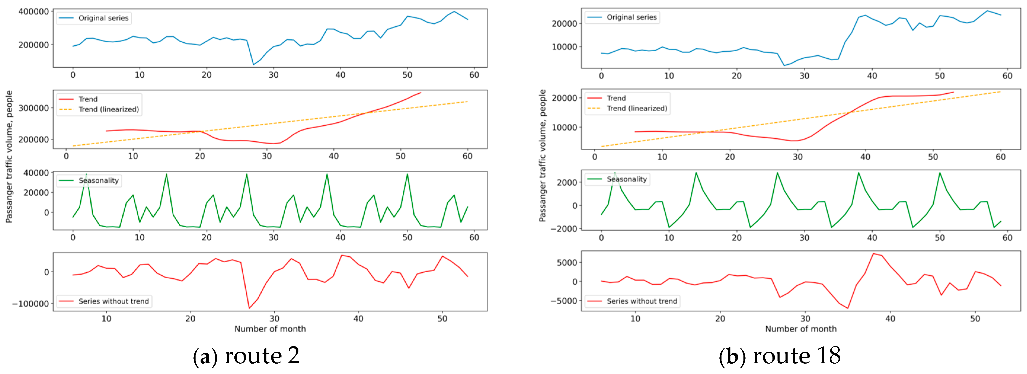
For the trend lines for routes 2, 18, 30, and 97, the correlation coefficients are statistically significant, and R² values are equal to or greater than 0.4. This indicates a significant trend in passenger traffic volume, which is increasing for routes 2 and 18 and decreasing for routes 30 and 97. Near-zero R² values for routes 91 and 134, as well as high MSE values, indicate the absence of long-term trends in passenger traffic volume, meaning the number of passengers carried for these routes is stable year-over-year. Figure 4, Figure 5 and Figure 6 present a harmonic analysis of the time series of passenger volumes for the routes in Table 1.

The top graph shows the original time series, followed by the trend and its approximation using a linear regression model. Next is a graph of seasonal fluctuations in the observed value, and finally, the detrended time series. All analyzed routes exhibited a decrease in passenger volumes in 2020, during the COVID-19 pandemic, reflected as a “dip” in the trend line graphs. To determine the impact of the COVID-19 pandemic on the trend component of the time series of the number of passengers carried by public transport, the statistical significance of the coefficients of the linear trend equation was assessed with and without taking into account the data for 2020 (the acute phase of the pandemic) using Student’s t-test. Using route No. 2 as an example, for both cases, the actual values of the t-test for the absolute term (b) and the linear regression coefficient (w) of the trend are 13.9 and 6.64 when including 2020, and 19.1 and 10.0 when excluding 2020. These values exceed the tabular values at a significance level of p = 0.99 (t_59;0.99 = 2.66 and t_47;0.99 = 2.68). The significance of other routes was assessed similarly. The results showed that restrictions on movement during the COVID-19 pandemic did not affect the nature of changes in long-term trends in the number of passengers transported on the routes under consideration.

The seasonal component of the time series for each route was determined using harmonic linearization. The number of a statistically significant harmonic corresponds to the period of time series oscillations. The statistical significance of the linearized harmonics was assessed using Student’s t-test. The characteristics of harmonic models for routes No. 2 and No. 30 are presented in

Table 3. Characteristics of harmonic models of passenger transport volumes.

No.	Route No.	Harmonic No.	Half-Amplitude of Oscillation	Initial Phase, Months	r2	r	tr
1	2	1	10,084.43	1.07	0.21	0.4583	1.63
2		2	13,836.64	6.42	0.4	0.6325	2.58
3		3	4974.72	7.62	0.05	0.2236	0.72
4		4	10,466.70	0.77	0.22	0.4690	1.68
5		5	7244.02	1.60	0.1	0.3162	1.05
6	30	1	12,731.83	9.43	0.02	0.1414	0.45
7		2	75,542.75	8.43	0.81	0.9000	6.52
8		3	12,506.99	5.35	0.02	0.1414	0.45
9		4	19,561.67	0.99	0.05	0.2236	0.72
10		5	23,954.16	0.95	0.08	0.2828	0.93

. If the calculated t-statistic for a harmonic is greater than the tabulated value (t_r > t_0.95), it is considered statistically significant. Thus, for routes No. 2, No. 18, and No. 30, the second harmonic with a ½-year oscillation period is statistically significant. This means that these routes experience two peaks in passenger traffic, typically associated with the spring and fall. The first peak corresponds to February–March, and the second to September.

For routes 97 and 134, the first harmonic with a 1-year oscillation period is statistically significant; peak traffic occurs in the summer. For route 91, the first and second harmonics are statistically significant, indicating the presence of repeating oscillations in the time series once a year (summer–fall) and twice a year in February and September.

After data processing, the parameters of the harmonic model in Equation (9) were obtained for all public transport routes. Examples of the harmonic model for changes in the number of public transport passengers for two routes, No. 30 and No. 2, are shown in Equations (10) and (11), respectively.

Y₃₀ = 598,713 + 75,542 × cos(30 × (2 × T − 8.43)).

(10)

Y₂ = 264,225 + 13,836 × cos(30 × (2 × T − 6.42)).

(11)

For a more accurate assessment of the performance of the urban public transportation system, including the efficiency of rolling stock on individual routes and the urban transportation system as a whole, all routes were grouped into classes using a clustering procedure. All five public transportation routes with an increasing trend are partially located in areas of the city where new residential complexes have been built, commissioned, or are under construction in the last three years, and where population density is increasing. The relationship between public transportation routes 2, 18, 33, and 100 with an increasing trend and areas under development in the northwestern and southwestern parts of the city is shown in

Table 4. The ratio of routes from the group with an increasing trend in traffic volume to the areas of the city under development.

No.	Route No.	Area Under Development
1	2	northwestern part of the city
2	18	northwestern part of the city
3	33	northwestern part of the city
4	100	southwestern part of the city
5	144	northwestern part of the city

and Figure 7, Figure 8 and Figure 9.

Based on the obtained clustering of the passenger transport routes, a set of measures was formed for each cluster to improve passenger transport in order to adjust the transport macromodel during the development and adjustment of transport planning documents and activities for organizing transport services for the city’s population.

When considering population mobility, it is necessary to comprehensively consider other modes of transportation and travel options. In addition to public transportation, private vehicles play a crucial role in providing transit services. When traveling to the city center for work in private cars, the main problem is a lack of parking spaces.

3.2. Analysis of the Temporal Unevenness in the Operation of Parking Spaces

Data on paid parking operations and parking sessions were aggregated by day, week, and month to create a time series of key metrics: total parking time (minutes) and occupancy rate (%). The average parking duration was 143.8 min (~2.4 h), typical for parking in the city’s business and administrative districts. Monthly occupancy rates ranged from 40.7% to 69.3%, averaging 54%.

When studying the performance of paid parking, seasonal peaks and cyclical patterns are evident. Figure 10 shows the pattern of changes in the number of parking sessions (Figure 10a) and parking occupancy (Figure 10b) in the central part of the city in the administrative and business district.

The minimum number of parking sessions occurs in January, while the maximum occurs in July/August, April, and October. Three peaks with maximum values can be identified for the time series of parking sessions: March/April, July/August, and October. The minimum peaks occur in November/December/January. A slight decrease is also observed during the periods May/June and September. Thus, similar to public transport passenger volumes, there is seasonal unevenness in passenger car parking throughout the year. To determine the seasonal fluctuations of the time series and the coefficients of the harmonic model approximating it, the harmonics were linearized, and the values of the correlation coefficients r of the linear regression models, as well as their statistical significance, were determined. The patterns of change in the response function by month for each of the five linearized harmonics are shown in Figure 11, and a comparison of the calculated and tabulated values of t-statistics is provided in

Table 5. Evaluation of the statistical significance of linearized harmonics for determining the period of oscillations of a time series.

Harmonic No.	Half-Amplitude of Oscillation	Initial Phase, Months	r2	r	tr	t0.95
1	1067.7	6.59	0.746	0.864	5.42	2.23
2	375.0	7.03	0.092	0.303	1.01
3	209.3	8.06	0.028	0.167	0.54
4	236.9	4.95	0.036	0.190	0.61
5	355.6	10.92	0.082	0.286	0.94

.

The correlation coefficient for the first harmonic is statistically significant, since t_r > t_0.95, i.e., 5.42 > 2.23. Consequently, the time series has significant seasonal fluctuations with a period of 1 year, the peak of which occurs in the summer months. The half-amplitude of the oscillation A_Y1 = 1067.68, and the initial phase T₀₁ = 6.59. These values can be substituted into (9) to obtain a model of the pattern of change in the response function over time.

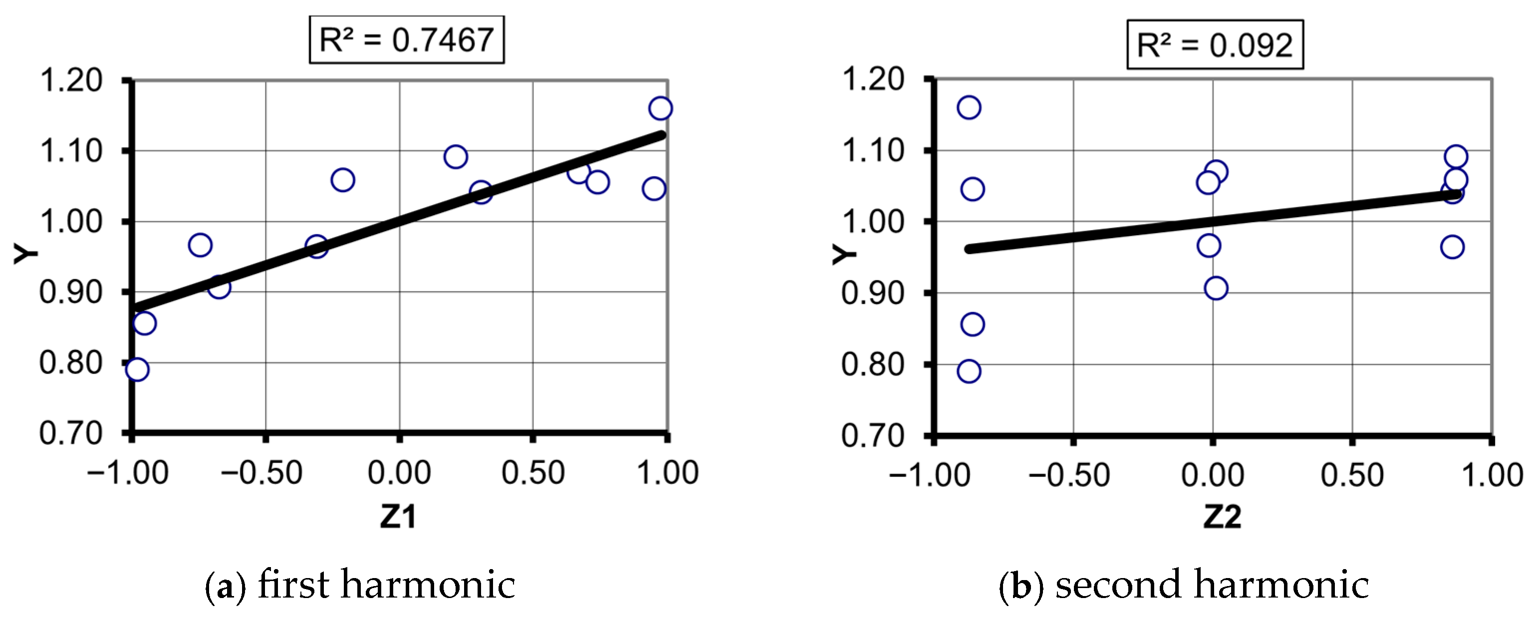
Figure 12 shows the multiple determination coefficients for the first two of the five linearized harmonics Z_1–5.

Equation (12) shows the harmonic model of the change in the number of parking sessions of cars in one of the central parking lots of the city.

Y₃₀ = Y₀ + 1067 × cos(30 × (2 × T − 6.59)).

(12)

The peak in parking sessions in July is driven by short-term trips for cultural and leisure purposes (visiting recreational areas, cafes, parks, museums, and movie theatres during the comfortable warm summer months). Furthermore, the total parking occupancy time in summer is shorter than in other periods, especially in fall (Figure 13).

A stationarity analysis of the daily parking usage time series (in minutes) was conducted. The Dickey–Fuller test was used. It tests the null hypothesis (H0) that the time series contains a unit root (i.e., it is non-stationary). The test rejected the unit root hypothesis. The original time series is stationary with a very high degree of confidence (significance level of 1%).

The test was then applied to the residuals (noise component) obtained after removing trend and seasonality from the original series (decomposition). The test statistic (−8.41) is extremely low and well below all critical values; the p-value is practically zero, providing compelling evidence to reject the null hypothesis. It can be concluded that the residuals are stationary. This means that the decomposition model (additive or multiplicative) adequately captured all non-stationary components (trend and seasonality). No systematic patterns remained in the residuals, only random noise. The residuals are stationary, but are not white noise. They exhibit extremely high volatility and a distribution significantly different from normality.

The following conclusions can be drawn:

• Methods assuming normality are undesirable for constructing forecast confidence intervals.
• The series may contain outliers or varying variance.

The data residuals exhibit abnormally high volatility and a non-normal distribution. This is a serious caveat for forecasting: point forecasts may be accurate, but the uncertainty around those forecasts will be extremely unreliable using standard methods.

The statistical significance of harmonics directly translates into practical tools for traffic flow management. Identifying seasonal fluctuations in a non-stationary time series of changes in the number of parking sessions and the occupancy rate of paid parking lots allows us to identify periods of peak and trough occupancy throughout the year. This allows for a transition from reactive to proactive parking space management, including through economic parameters and the level of service to car owners. One management measure is the application of differentiated parking rates throughout the year, which allows for more flexible parking space management. When demand is low, lowering rates can increase the number and duration of parking sessions, thereby increasing municipal revenues. When demand is high, raising rates can reduce the number of trips and, consequently, traffic congestion in paid parking zones. All of this combined makes the parking system more adaptive to changing conditions and ensures sustainable mobility. Knowledge of time series on the number and duration of parking sessions will allow us to make refinements to the transport supply model (via the counting location attribute) and evaluate the accuracy of the city’s macromodel when determining the parameters of the transport system for different periods of the year.

Transport demand and the number of personal car trips are managed through a number of measures, including paid parking rates. To evaluate the effectiveness of measures within the Mobility as a Service (MaaS) concept, it is necessary to identify patterns and trends in paid parking occupancy.

Parking session forecasting was conducted using two methods: SARIMA (Seasonal ARIMA) and Prophet.

Training set: parking session data for the period 11 January 2023–31 December 2024;

Test sample: 1 January 2025–28 March 2025.

Evaluation of the forecast quality on test data:

SARIMA-MAE: 17,135.27, RMSE: 18,811.94;

Prophet-MAE: 5644.03, RMSE: 8948.69.

The Prophet model proved to be the most accurate in predicting the occupancy rate of this parking lot. This is due to a number of factors that distinguish this model from SARIMA: it takes into account multiple seasonalities (e.g., weekly and annual); reduces the impact of outliers; and takes into account local events (changes in tariffs, openings of new parking areas, city events, etc.). However, the Prophet model also has a number of limitations: it is less effective for very short series (<1 seasonal cycle); it assumes additivity of components (may not work for multiplicative patterns). The forecast results show a gradual, slight decline in the number of parking sessions in the remaining months of 2025 (Figure 14).

This is due to a number of factors: rising parking costs at the location where data were collected, the expansion of paid parking zones, and residents using other paid parking lots with lower rates. To improve forecast accuracy, it is necessary to conduct an analysis of all paid parking lots in the city, taking into account not only temporal but also spatial variations, as well as rate changes over the past 3–5 years.

When implementing the research results, we plan to use a combined approach and integrate both methods into the transport system forecasting module. The Prophet method will be used for operational forecasting, while the SARIMA method will be used to analyze stable demand components. This will enable the creation of a more comprehensive system for analyzing and forecasting parking infrastructure operations.

4. Discussion

This study solved a scientific problem of determining the temporal unevenness of passenger traffic on individual public transportation routes and paid parking sessions. Three groups of public transportation routes with different trends in passenger traffic volumes were identified. It was established that the increasing trends (on certain public transport routes) are determined by the development of individual city areas. Furthermore, changes in the transport system operating parameters over time are determined by the spatial characteristics of public transportation routes (length and non-linearity of the route) and the development of individual city areas.

Knowledge of the various trends in passenger traffic volume allows for differentiated approaches to optimizing and improving the efficiency of rolling stock operations on routes and ways to improve the quality of public transportation services.

Understanding patterns of passenger traffic volume changes throughout the year (cyclicity) on individual routes and the trends in this indicator can be applied in several ways. First, it is used to consider the number of trips, schedules, and distribution of rolling stock of different passenger capacity classes across the routes in long-term planning documents for scheduled transportation, and to adjust documents during operational management. Second, it is used in the operational management of a company engaged in urban ground public transportation along the routes when planning the rate of vehicle operation (buses, trolleybuses) to calculate driver working time, plan employee vacations, and maintain a stock of parts and materials for vehicle maintenance and repair.

Further research has been identified, using the established patterns to develop a set of measures to improve the efficiency of vehicle operation on routes and the overall ground public transportation system when reaching the maximum criteria for passenger volume. Additionally, when the volume of transportation changes, it is possible and advisable to adjust not only the number and class of vehicles on the routes, but also the public transport infrastructure, including optimizing the parameters, number, and location of bus stops and transport hubs, and the availability of lanes for public transport.

Trends and cyclical patterns in passenger traffic volume on routes can be one of the criteria for selecting a management method for a transport complex subsystem:

• Revising route groups in lots during municipal tenders for passenger transportation on urban routes;
• Forming holdings from carriers to create a common reserve of buses to compensate for service disruptions due to various reasons (vehicle malfunction, driver illness, other organizational issues), during the procurement of new additional buses (during system development), and renewal of rolling stock;
• Creating more flexible terms in municipal contracts for adjusting contract parameters for routes with a declining trend based on passenger traffic volume;
• Introducing this parameter into the list of calculation parameters in digital twins of cities and intelligent transport systems;
• Introducing conditions for activating route optimization procedures in the operating algorithms of digital twins of cities and intelligent transport systems when specified threshold deviations for the passenger traffic volume parameter are reached, including by changing the carrying capacity or route. For example, if traffic volumes increase and passenger flow changes on certain route sectors, additional trips on shorter routes may be introduced. If traffic volumes decrease, some trips may be transferred to shorter routes.

Understanding the temporal unevenness of paid parking occupancy and the characteristics of parking sessions allows us to develop a methodology and standards for dynamic parking rates (changing throughout the day) for passenger cars. Studying the spatial and temporal unevenness of public transportation and paid parking occupancy will enable us to differentiate measures to improve the efficiency of public transportation management, parking space, and the overall transportation system. The implementation of measures to ensure sustainable urban mobility requires financial resources from municipal or regional budgets. At the same time, the effectiveness of individual measures may differ significantly for different transport areas, taking into account their location, and requires detailed elaboration in transport planning documents.

Future research focuses on integrating the established time series and methods for forecasting passenger transport and parking volumes into the city’s estimated digital twin. Incorporating a module for forecasting medium-term parameter changes into the transport system’s digital twin will enable the creation of an automated decision-making system and improve the efficiency of city management.

References

1. Burrows, A.; Bradburn, J.; Cohen, T. Journeys of the Future. Introducing Mobility as a Service; Atkins Global: Singapore, 2015; p. 36. [Google Scholar]
2. Turoń, K. Sustainable Urban Mobility Transitions—From Policy Uncertainty to the CalmMobility Paradigm. Smart Cities 2025, 8, 164. [Google Scholar] [CrossRef]
3. Arliansyah, J.; Prasetyo, M.R.; Kurnia, A.Y. Planning of city transportation infrastructure based on macro simulation model. Int. J. Adv. Sci. Eng. Inf. Technol. 2017, 7, 1262–1267. [Google Scholar] [CrossRef]
4. Currie, G.; Gruyter, D. Exploring links between the sustainability performance of urban public transport and land use in international cities. J. Transp. Land Use 2018, 11, 325–342. [Google Scholar] [CrossRef]
5. Almansoub, Y.; Zhong, M.; Raza, A.; Safdar, M.; Dahou, A.; Al-qaness, M.A.A. Exploring the Effects of Transportation Supply on Mixed Land-Use at the Parcel Level. Land 2022, 11, 797. [Google Scholar] [CrossRef]
6. Bao, L.; Kusadokoro, M.; Chitose, A.; Chen, C. Development of socially sustainable transport research: A bibliometric and visualization analysis. Travel Behav. Soc. 2023, 30, 60–73. [Google Scholar] [CrossRef]
7. Chainikov, D.; Zakharov, D.; Kozin, E.; Pistsov, A. Studying Spatial Unevenness of Transport Demand in Cities Using Machine Learning Methods. Appl. Sci. 2024, 14, 3220. [Google Scholar] [CrossRef]
8. Davis, G.A.; Nihan, N.L. Using Time-Series Designs to Estimate Changes in Freeway Level of Service, despite Missing Data. Transp. Res. Part A Gen. 1984, 18, 431–438. [Google Scholar] [CrossRef]
9. Cui, X.; Lv, H. STEFT: Spatio-Temporal Embedding Fusion Transformer for Traffic Prediction. Electronics 2024, 13, 3816. [Google Scholar] [CrossRef]
10. Yu, C.; Dong, W.; Lin, H.; Lu, Y.; Wan, C.; Yin, Y.; Qin, Z.; Yang, C.; Yuan, Q. Multi-layer regional railway network and equitable economic development of megaregions. Sustain. Mobil. Transp. 2025, 2, 3. [Google Scholar] [CrossRef]
11. Dabiri, S.; Heaslip, K. Inferring transportation modes from GPS trajectories using a convolutional neural network. Transp. Res. Part C Emerg. Technol. 2018, 86, 360–371. [Google Scholar] [CrossRef]
12. Zhang, J.; Zheng, Y.; Qi, D. Deep spatio-temporal residual networks for citywide crowd flows prediction. Proc. AAAI Conf. Artif. Intell. 2016, 31, 1655–1661. [Google Scholar] [CrossRef]
13. Yang, H.; Xie, K.; Ozbay, K.; Ma, Y.; Wang, Z. Use of deep learning to predict daily usage of bike sharing systems. Transp. Res. Rec. 2018, 2672, 92–102. [Google Scholar] [CrossRef]
14. Chung, J.; Sohn, K. Image-based learning to measure trac density using a deep convolutional neural network. IEEE Trans. Intell. Transp. Syst. 2017, 19, 1670–1675. [Google Scholar] [CrossRef]
15. Roszkowska, E.; Filipowicz-Chomko, M.; Górecka, D.; Majewska, E. Sustainable Cities and Communities in EU Member States: A Multi-Criteria Analysis. Sustainability 2025, 17, 22. [Google Scholar] [CrossRef]
16. Petrov, A.I.; Petrova, D.A. Sustainability of Transport System of Large Russian City in the Period of COVID-19: Methods and Results of Assessment. Sustainability 2020, 12, 7644. [Google Scholar] [CrossRef]
17. Al-Akioui, A.; Monzon, A. Spatial Analysis of COVID-19 Pandemic Impacts on Mobility in Madrid Region. Sustainability 2023, 15, 14259. [Google Scholar] [CrossRef]
18. Guo, W.; Feng, Y.; Luo, W.; Ren, Y.; Tan, J.; Jiang, X.; Xue, Q. The Impacts of COVID-19 and Policies on Spatial and Temporal Distribution Characteristics of Traffic: Two Examples in Beijing. Sustainability 2022, 14, 1733. [Google Scholar] [CrossRef]
19. Hernandez, J.E.B.; Torres, L.E.T.; Tabare, A.; Álvarez-Martínez, D. Optimization of Bus Dispatching in Public Transportation Through a Heuristic Approach Based on Passenger Demand Forecasting. Smart Cities 2025, 8, 87. [Google Scholar] [CrossRef]
20. Babapourdijojin, M.; Corazza, M.V.; Gentile, G. Systematic Analysis of Commuting Behavior in Italy Using K-Means Clustering and Spatial Analysis: Towards Inclusive and Sustainable Urban Transport Solutions. Future Transp. 2024, 4, 1430–1456. [Google Scholar] [CrossRef]
21. Filippi, F. Visions, Paradigms, and Anomalies of Urban Transport. Future Transp. 2024, 4, 938–967. [Google Scholar] [CrossRef]
22. Kou, W.; Zhang, S.; Liu, F.; Pang, L. Dynamic Optimization of Exclusive Bus Lane Location Considering Reliability: A Case Study of Beijing. Appl. Sci. 2024, 14, 9777. [Google Scholar] [CrossRef]
23. Owen, D.; Arribas-Bel, D.; Rowe, F. Tracking the Transit Divide: A Multilevel Modelling Approach of Urban Inequalities and Train Ridership Disparities in Chicago. Sustainability 2023, 15, 8821. [Google Scholar] [CrossRef]
24. Korzen, M.; Kruszyna, M. Public Transport Planning Using Modified Ant Colony Optimization. Sustainability 2025, 17, 2468. [Google Scholar] [CrossRef]
25. Carreyre, F.; Chouaki, T.; Coulombel, N.; Berrada, J.; Hörl, S. Beyond Traditional Public Transport: A Cost–Benefit Analysis of First and Last-Mile AV Solutions in Periurban Environment. Sustainability 2025, 17, 6282. [Google Scholar] [CrossRef]
26. Zheng, H.; Zhang, X.; Chen, J. Study on Customized Shuttle Transit Mode Responding to Spatiotemporal Inhomogeneous Demand in Super-Peak. Information 2021, 12, 429. [Google Scholar] [CrossRef]
27. Wang, H.; Zeng, W. Revealing Urban Carbon Dioxide (CO2) Emission Characteristics and Influencing Mechanisms from the Perspective of Commuting. Sustainability 2019, 11, 385. [Google Scholar] [CrossRef]
28. Zhao, J.; Kong, W.; Zhou, M.; Zhou, T.; Xu, Y.; Li, M. Prediction of Urban Taxi Travel Demand by Using Hybrid Dynamic Graph Convolutional Network Model. Sensors 2022, 22, 5982. [Google Scholar] [CrossRef]
29. Gao, Y.; Zhu, J. Characteristics, Impacts and Trends of Urban Transportation. Encyclopedia 2022, 2, 1168–1182. [Google Scholar] [CrossRef]
30. Narayanan, S.; Makarov, N.; Antoniou, C. Graph Neural Networks as Strategic Transport Modelling Alternative—A Proof of Concept for a Surrogate. IET Intell. Transp. Syst. 2024, 18, 2059–2077. [Google Scholar] [CrossRef]
31. Ma, X.; Yu, H.; Wang, Y. Large-Scale Transportation Network Congestion Evolution Prediction Using Deep Learning Theory. PLoS ONE 2015, 10, e0119044. [Google Scholar] [CrossRef] [PubMed]
Figure 1. Distribution of medium load by route categories.
Sustainability 18 00225 g001
Figure 2. Diagram of the most and least loaded routes.
Sustainability 18 00225 g002
Figure 3. Distribution of the Dickey–Fuller test p-value by routes.
Sustainability 18 00225 g003
Figure 4. Harmonic analysis of passenger traffic volume on routes with an increasing trend.
Sustainability 18 00225 g004
Figure 5. Harmonic analysis of passenger traffic volume on routes with a downward trend.
Sustainability 18 00225 g005
Figure 6. Harmonic analysis of passenger traffic volume on routes with stable traffic volume.
Sustainability 18 00225 g006
Figure 7. The relative location of public transport routes with an increasing trend in passenger traffic volume and areas with increasing population density.
Sustainability 18 00225 g007
Figure 8. Development of the southwestern part of the city. Photo by authors via Yandex Maps.
Sustainability 18 00225 g008
Figure 9. Development of the northwestern part of the city. Photo by authors via Yandex Maps.
Sustainability 18 00225 g009
Figure 10. Changes in the number of paid parking sessions from January 2023 to March 2025.
Sustainability 18 00225 g010
Figure 11. Graph of the decomposition of the time series Yc into five harmonics, as well as the approximation line of the calculated value of the Yemp indicator by the harmonic model.
Sustainability 18 00225 g011
Figure 12. Values of the coefficients of multiple determination for the first two linearized harmonics Z1–Z2.
Sustainability 18 00225 g012
Figure 13. Decomposition of a time series of daily parking usage (in minutes) into trend, seasonality, and residual.
Sustainability 18 00225 g013
Figure 14. Forecasting the change in the number of paid parking sessions during 2025.
Sustainability 18 00225 g014