
TeaNet: An Enhanced Attention Network for Climate-Resilient River Discharge Forecasting Under CMIP6 SSP585 Projections

 , ,
, ,  , , , , ,
Abstract
1. Introduction
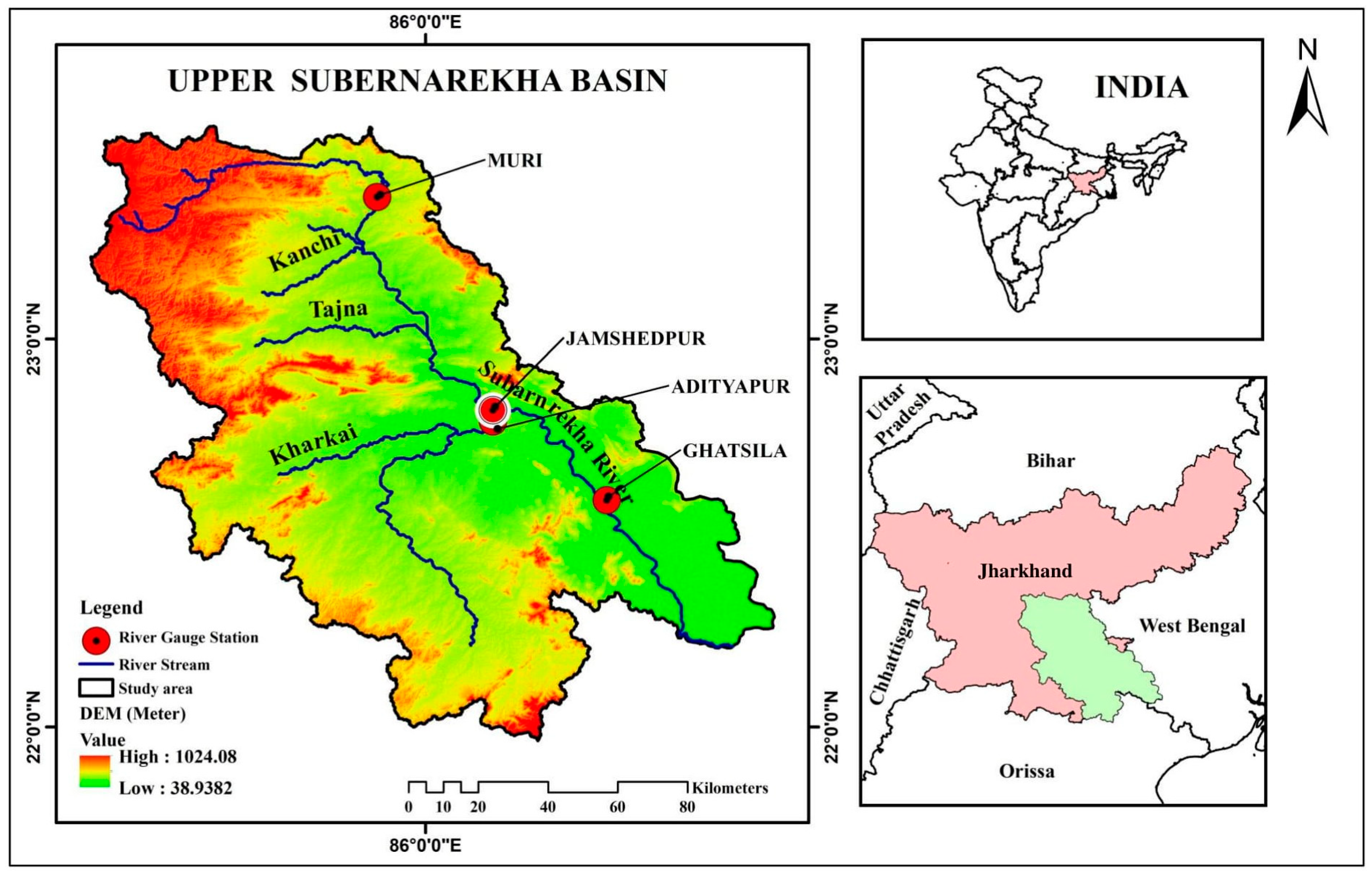
2. Study Area
3. Materials and Methodology
3.1. Data and Methods
3.1.1. Hydroclimatic Data
3.1.2. Data Pre-Processing
- Bias correction of GCM models
3.2. Methodology
3.2.1. Regression Models
- Temporal Convolutional Network (TCN)
- Random Forest (RF)
- Gated Recurrent Unit (GRU)
- Support Vector Regression (SVR)
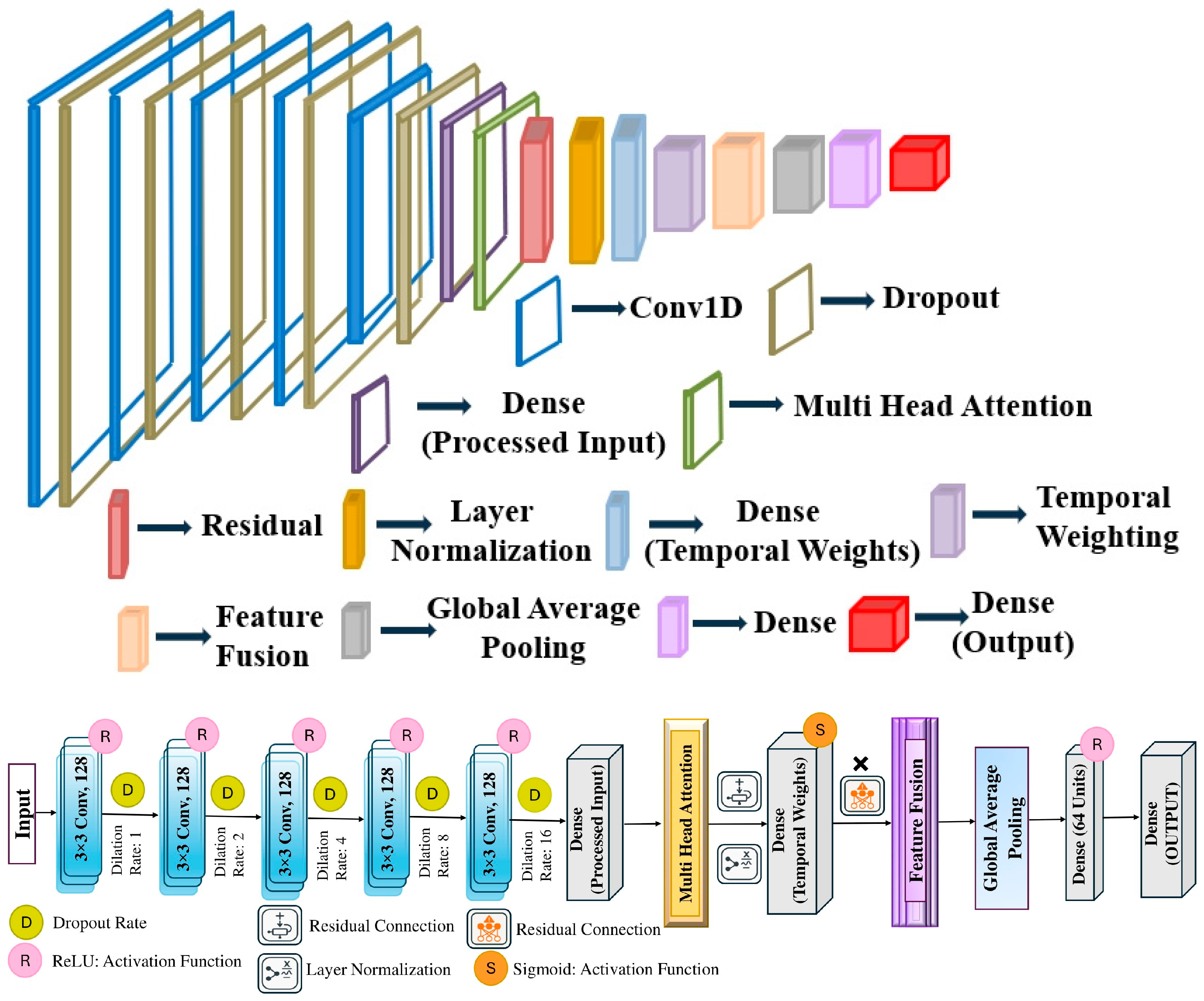
- Temporal Enhanced Attention Network (TeaNet)
3.2.2. Feature Importance Using TeaNet Model
3.2.3. Performance Assessment
4. Results and Discussion
4.1. Multi-Model Ensemble of General Circulation Models
4.2. Analysis of Regression Models’ Performance
4.3. Results Regarding Feature Importance Using TeaNet
4.4. Futuristic River Discharge Predictions Under the SSP585 Scenario
4.5. Implications for Water Resource Management and Flood Risk Mitigation
4.6. Uncertainty Analysis and Model Limitations
5. Conclusions
Supplementary Materials
Author Contributions
Funding
Institutional Review Board Statement
Informed Consent Statement
Data Availability Statement
Acknowledgments
Conflicts of Interest
References
- Ferrelli, F.; Pontrelli Albisetti, M.; Brendel, A.S.; Casoni, A.I.; Hesp, P.A. Appraisal of Daily Temperature and Rainfall Events in the Context of Global Warming in South Australia. Water 2024, 16, 351. [Google Scholar] [CrossRef]
- Khan, Z.; Khan, F.A.; Khan, A.U.; Hussain, I.; Khan, A.; Shah, L.A.; Khan, J.; Badrashi, Y.I.; Kamiński, P.; Dyczko, A.; et al. Climate-Streamflow Relationship and Consequences of Its Instability in Large Rivers of Pakistan: An Elasticity Perspective. Water 2022, 14, 2033. [Google Scholar] [CrossRef]
- Singh, D.; Vardhan, M.; Sahu, R.; Chatterjee, D.; Chauhan, P.; Liu, S. Machine-Learning- and Deep-Learning-Based Streamflow Prediction in a Hilly Catchment for Future Scenarios Using CMIP6 GCM Data. Hydrol. Earth Syst. Sci. 2023, 27, 1047–1075. [Google Scholar] [CrossRef]
- Gerten, D.; Rost, S.; von Bloh, W.; Lucht, W. Causes of Change in 20th Century Global River Discharge. Geophys. Res. Lett. 2008, 35, 20405. [Google Scholar] [CrossRef]
- Nepal, S.; Shrestha, A.B. Impact of Climate Change on the Hydrological Regime of the Indus, Ganges and Brahmaputra River Basins: A Review of the Literature. Int. J. Water Resour. Dev. 2015, 31, 201–218. [Google Scholar] [CrossRef]
- Nilawar, A.P.; Waikar, M.L. Impacts of Climate Change on Streamflow and Sediment Concentration under RCP 4.5 and 8.5: A Case Study in Purna River Basin, India. Sci. Total Environ. 2019, 650, 2685–2696. [Google Scholar] [CrossRef] [PubMed]
- Meehl, G.A.; Moss, R.; Taylor, K.E.; Eyring, V.; Stouffer, R.J.; Bony, S.; Stevens, B. Climate Model Intercomparisons: Preparing for the Next Phase. Eos Trans. Am. Geophys. Union 2014, 95, 77–78. [Google Scholar] [CrossRef]
- Zhang, G. Improve Climate Predictions by Reducing Initial Prediction Errors: A Benefit Estimate Using Multi-Model ENSO Predictions. ESS Open Arch. 2023; in press. [Google Scholar] [CrossRef]
- Li, G.; Xie, S.-P.; He, C.; Chen, Z. Western Pacific Emergent Constraint Lowers Projected Increase in Indian Summer Monsoon Rainfall. Nat. Clim. Chang. 2017, 7, 708–712. [Google Scholar] [CrossRef]
- Aghakhani Afshar, A.; Hasanzadeh, Y.; Besalatpour, A.A.; Pourreza-Bilondi, M. Climate Change Forecasting in a Mountainous Data Scarce Watershed Using CMIP5 Models under Representative Concentration Pathways. Theor. Appl. Climatol. 2017, 129, 683–699. [Google Scholar] [CrossRef]
- Kamal, A.S.M.M.; Hossain, F.; Shahid, S. Spatiotemporal Changes in Rainfall and Droughts of Bangladesh For1.5 and 2 °C Temperature Rise Scenarios of CMIP6 Models. Theor. Appl. Climatol. 2021, 146, 527–542. [Google Scholar] [CrossRef]
- Khan, N.; Shahid, S.; Ahmed, K.; Wang, X.; Ali, R.; Ismail, T.; Nawaz, N. Selection of GCMs for the Projection of Spatial Distribution of Heat Waves in Pakistan. Atmos. Res. 2020, 233, 104688. [Google Scholar] [CrossRef]
- Su, B.; Huang, J.; Mondal, S.K.; Zhai, J.; Wang, Y.; Wen, S.; Gao, M.; Lv, Y.; Jiang, S.; Jiang, T.; et al. Insight from CMIP6 SSP-RCP Scenarios for Future Drought Characteristics in China. Atmos. Res. 2021, 250, 105375. [Google Scholar] [CrossRef]
- Gusain, A.; Ghosh, S.; Karmakar, S. Added Value of CMIP6 over CMIP5 Models in Simulating Indian Summer Monsoon Rainfall. Atmos. Res. 2020, 232, 104680. [Google Scholar] [CrossRef]
- Xin, X.; Wu, T.; Zhang, J.; Yao, J.; Fang, Y. Comparison of CMIP6 and CMIP5 Simulations of Precipitation in China and the East Asian Summer Monsoon. Int. J. Climatol. 2020, 40, 6423–6440. [Google Scholar] [CrossRef]
- Srivastava, A.; Grotjahn, R.; Ullrich, P.A. Evaluation of Historical CMIP6 Model Simulations of Extreme Precipitation over Contiguous US Regions. Weather. Clim. Extrem. 2020, 29, 100268. [Google Scholar] [CrossRef]
- Mahmood, R.; Babel, M.S. Evaluation of SDSM Developed by Annual and Monthly Sub-Models for Downscaling Temperature and Precipitation in the Jhelum Basin, Pakistan and India. Theor. Appl. Climatol. 2013, 113, 27–44. [Google Scholar] [CrossRef]
- Hassan, I.; Kalin, R.M.; White, C.J.; Aladejana, J.A. Selection of CMIP5 GCM Ensemble for the Projection of Spatio-Temporal Changes in Precipitation and Temperature over the Niger Delta, Nigeria. Water 2020, 12, 385. [Google Scholar] [CrossRef]
- Salehie, O.; Hamed, M.M.; Ismail, T.B.; Tam, T.H.; Shahid, S. Selection of CMIP6 GCM with Projection of Climate over the Amu Darya River Basin. Theor. Appl. Climatol. 2023, 151, 1185–1203. [Google Scholar] [CrossRef]
- Ahmed, K.; Sachindra, D.A.; Shahid, S.; Demirel, M.C.; Chung, E.S. Selection of Multi-Model Ensemble of General Circulation Models for the Simulation of Precipitation and Maximum and Minimum Temperature Based on Spatial Assessment Metrics. Hydrol. Earth Syst. Sci. 2019, 23, 4803–4824. [Google Scholar] [CrossRef]
- Haleem, K.; Khan, A.U.; Khan, J.; Ghanim, A.A.J.; Al-Areeq, A.M. Evaluating Future Streamflow Patterns under SSP245 Scenarios: Insights from CMIP6. Sustainability 2023, 15, 16117. [Google Scholar] [CrossRef]
- Zhang, S.; Gan, T.Y.; Bush, A.B.G.; Zhang, G. Evaluation of the Impact of Climate Change on the Streamflow of Major Pan-Arctic River Basins through Machine Learning Models. J. Hydrol. 2023, 619, 129295. [Google Scholar] [CrossRef]
- Yang, Q.; Zhang, H.; Wang, G.; Luo, S.; Chen, D.; Peng, W.; Shao, J. Dynamic Runoff Simulation in a Changing Environment: A Data Stream Approach. Environ. Model. Softw. 2019, 112, 157–165. [Google Scholar] [CrossRef]
- Fu, M.; Fan, T.; Ding, Z.; Salih, S.Q.; Al-Ansari, N.; Yaseen, Z.M. Deep Learning Data-Intelligence Model Based on Adjusted Forecasting Window Scale: Application in Daily Streamflow Simulation. IEEE Access 2020, 8, 32632–32651. [Google Scholar] [CrossRef]
- Ghobadi, F.; Kang, D. Improving Long-Term Streamflow Prediction in a Poorly Gauged Basin Using Geo-Spatiotemporal Mesoscale Data and Attention-Based Deep Learning: A Comparative Study. J. Hydrol. 2022, 615, 128608. [Google Scholar] [CrossRef]
- Rahimzad, M.; Moghaddam Nia, A.; Zolfonoon, H.; Soltani, J.; Danandeh Mehr, A.; Kwon, H.H. Performance Comparison of an LSTM-Based Deep Learning Model versus Conventional Machine Learning Algorithms for Streamflow Forecasting. Water Resour. Manag. 2021, 35, 4167–4187. [Google Scholar] [CrossRef]
- Marqas, R.B.; Almufti, S.M.; Asaad, R.R.; Mohamed, T.S. Advancing AI: A Comprehensive Study of Novel Machine Learning Architectures. Int. J. Sci. World 2025, 11, 48–85. [Google Scholar] [CrossRef]
- Moya, H.; Althoff, I.; Celis-Diez, J.L.; Huenchuleo-Pedreros, C.; Reggiani, P. Impact of Future Climate Scenarios and Bias Correction Methods on the Achibueno River Basin. Water 2024, 16, 1138. [Google Scholar] [CrossRef]
- Dingamadji, M.; Adounkpe, J.; Abderamane, H.; Abdallah, M.N. Bias Correction of CORDEX-Africa Regional Climate Model Simulations for Climate Change Projections in Northeastern Lake Chad: Comparative Analysis of Three Bias Correction Methods. Eur. Sci. J. ESJ 2024, 20, 204. [Google Scholar] [CrossRef]
- Semenov, M.A.; Senapati, N.; Coleman, K.; Collins, A.L. A Dataset of CMIP6-Based Climate Scenarios for Climate Change Impact Assessment in Great Britain. Data Brief 2024, 55, 110709. [Google Scholar] [CrossRef]
- Solanki, H.; Vegad, U.; Kushwaha, A.; Mishra, V. Improving Streamflow Prediction Using Multiple Hydrological Models and Machine Learning Methods. Water Resour. Res. 2025, 61, e2024WR038192. [Google Scholar] [CrossRef]
- Yaseen, Z.M. A New Benchmark on Machine Learning Methodologies for Hydrological Processes Modelling: A Comprehensive Review for Limitations and Future Research Directions. Knowl.-Based Eng. Sci. 2023, 4, 65–103. [Google Scholar] [CrossRef]
- Teweldebrhan, A.T.; Schuler, T.V.; Burkhart, J.F.; Hjorth-Jensen, M. Coupled Machine Learning and the Limits of Acceptability Approach Applied in Parameter Identification for a Distributed Hydrological Model. Hydrol. Earth Syst. Sci. 2020, 24, 4641–4658. [Google Scholar] [CrossRef]
- Puthukulangara, S. Comparative Analysis of Fall Detection Using Artificial Neural Networks (ANN) and K-Nearest Neighbors (KNN) Algorithms. Res. Rev. Mach. Learn. Cloud Comput. 2024, 3, 20–31. [Google Scholar] [CrossRef]
- Hoang, V.H.; Nguyen, N.L.; Bui, T.T.; Tran, N.H. A Two-Stage Method for Damage Detection in Z24 Bridge Based on K-Nearest Neighbor and Artificial Neural Network. Period. Polytech. Civ. Eng. 2024, 68, 892–902. [Google Scholar] [CrossRef]
- Sharma, S.; Kumari, S. River Discharge Forecasting in Mahanadi River Basin Based on Deep Learning Techniques. In Applications of Machine Learning in Hydroclimatology; Springer Nature: Cham, Switzerland, 2025; pp. 47–56. [Google Scholar]
- Hagemann, S.; Nguyen, T.T.; Ho-Hagemann, H.T.M. A Three-Quantile Bias Correction with Spatial Transfer for the Correction of Simulated European River Runoff to Force Ocean Models. Ocean. Sci. 2024, 20, 1457–1478. [Google Scholar] [CrossRef]
- Chao, Z.; Wang, H.; Hu, S.; Wang, M.; Xu, S.; Zhang, W. Permeability and Porosity of Light-Weight Concrete with Plastic Waste Aggregate: Experimental Study and Machine Learning Modelling. Constr. Build. Mater. 2024, 411, 134465. [Google Scholar] [CrossRef]
- Liu, J.; Bian, Y.; Lawson, K.; Shen, C. Probing the Limit of Hydrologic Predictability with the Transformer Network. J. Hydrol. 2024, 637, 131389. [Google Scholar] [CrossRef]
- Feng, D.; Beck, H.; Lawson, K.; Shen, C. The Suitability of Differentiable, Physics-Informed Machine Learning Hydrologic Models for Ungauged Regions and Climate Change Impact Assessment. Hydrol. Earth Syst. Sci. 2023, 27, 2357–2373. [Google Scholar] [CrossRef]
- Yang, R.; Wu, J.; Gan, G.; Guo, R.; Zhang, H. Combining Physical Hydrological Model with Explainable Machine Learning Methods to Enhance Water Balance Assessment in Glacial River Basins. Water 2024, 16, 3699. [Google Scholar] [CrossRef]
- Sharma, R.K.; Kumar, S.; Padmalal, D.; Roy, A. Streamflow Prediction Using Machine Learning Models in Selected Rivers of Southern India. Int. J. River Basin Manag. 2024, 22, 529–555. [Google Scholar] [CrossRef]
- Rather, S.A.; Patel, M.; Kapoor, K. AI-Driven Forecasting of River Discharge: The Case Study of the Himalayan Mountainous River. Earth Sci. Inform. 2025, 18, 242. [Google Scholar] [CrossRef]
- Gupta, D.B.; Mitra, S. Sustaining Subernarekha River Basin. Int. J. Water Resour. Dev. 2004, 20, 431–444. [Google Scholar] [CrossRef]
- Chatterjee, S.; Krishna, A.P.; Sharma, A.P. Geospatial Assessment of Soil Erosion Vulnerability at Watershed Level in Some Sections of the Upper Subarnarekha River Basin, Jharkhand, India. Environ. Earth Sci. 2014, 71, 357–374. [Google Scholar] [CrossRef]
- Tabassum, F.; Krishna, A.P. Spatio-Temporal Drought Assessment of the Subarnarekha River Basin, India, Using CHIRPS-Derived Hydrometeorological Indices. Environ. Monit. Assess. 2022, 194, 902. [Google Scholar] [CrossRef] [PubMed]
- Zhou, G.; Li, J.; Tian, Z.; Xu, J.; Bai, Y. The Extended Stumpf Model for Water Depth Retrieval from Satellite Multispectral Images. IEEE J. Sel. Top. Appl. Earth Obs. Remote Sens. 2024, 17, 6779–6790. [Google Scholar] [CrossRef]
- Pang, Q.; Zhao, G.; Wang, D.; Zhu, X.; Xie, L.; Zuo, D.; Wang, L.; Tian, L.; Peng, F.; Xu, B.; et al. Water periods impact the structure and metabolic potential of the nitrogen-cycling microbial communities in rivers of arid and semi-arid regions. Water Res. 2024, 267, 122472. [Google Scholar] [CrossRef]
- Teutschbein, C.; Seibert, J. Bias Correction of Regional Climate Model Simulations for Hydrological Climate-Change Impact Studies: Review and Evaluation of Different Methods. J. Hydrol. 2012, 456–457, 12–29. [Google Scholar] [CrossRef]
- Hakala, K.; Addor, N.; Teutschbein, C.; Vis, M.; Dakhlaoui, H.; Seibert, J. Hydrological Modeling of Climate Change Impacts. In Encyclopedia of Water; Wiley: Hoboken, NJ, USA, 2019; pp. 1–20. [Google Scholar]
- Li, R.; Chu, Z.; Jin, W.; Wang, Y.; Hu, X. Temporal Convolutional Network Based Regression Approach for Estimation of Remaining Useful Life. In Proceedings of the 2021 IEEE International Conference on Prognostics and Health Management (ICPHM), Detroit (Romulus), MI, USA, 7–9 June 2021; pp. 1–10. [Google Scholar]
- Georganos, S.; Kalogirou, S. A Forest of Forests: A Spatially Weighted and Computationally Efficient Formulation of Geographical Random Forests. ISPRS Int. J. Geoinf. 2022, 11, 471. [Google Scholar] [CrossRef]
- Gholami, H.; Mohammadifar, A.; Golzari, S.; Song, Y.; Pradhan, B. Interpretability of Simple RNN and GRU Deep Learning Models Used to Map Land Susceptibility to Gully Erosion. Sci. Total Environ. 2023, 904, 166960. [Google Scholar] [CrossRef]
- Panahi, M.; Sadhasivam, N.; Pourghasemi, H.R.; Rezaie, F.; Lee, S. Spatial Prediction of Groundwater Potential Mapping Based on Convolutional Neural Network (CNN) and Support Vector Regression (SVR). J. Hydrol. 2020, 588, 125033. [Google Scholar] [CrossRef]
- Zhang, X.; Chan, F.T.S.; Mahadevan, S. Explainable Machine Learning in Image Classification Models: An Uncertainty Quantification Perspective. Knowl. Based Syst. 2022, 243, 108418. [Google Scholar] [CrossRef]
- Niu, Z.; Zhong, G.; Yu, H. A Review on the Attention Mechanism of Deep Learning. Neurocomputing 2021, 452, 48–62. [Google Scholar] [CrossRef]
- Katipoğlu, O.M.; Sarıgöl, M. Coupling Machine Learning with Signal Process Techniques and Particle Swarm Optimization for Forecasting Flood Routing Calculations in the Eastern Black Sea Basin, Türkiye. Environ. Sci. Pollut. Res. 2023, 30, 46074–46091. [Google Scholar] [CrossRef]
- Ristea, E.; Bisinicu, E.; Lavric, V.; Parvulescu, O.C.; Lazar, L. A Long-Term Perspective of Seasonal Shifts in Nutrient Dynamics and Eutrophication in the Romanian Black Sea Coast. Sustainability 2025, 17, 1090. [Google Scholar] [CrossRef]
- Montràs-Janer, T.; Suggitt, A.J.; Fox, R.; Jönsson, M.; Martay, B.; Roy, D.B.; Walker, K.J.; Auffret, A.G. Anthropogenic Climate and Land-Use Change Drive Short- and Long-Term Biodiversity Shifts across Taxa. Nat. Ecol. Evol. 2024, 8, 739–751. [Google Scholar] [CrossRef]
- Meema, T.; Tachikawa, Y.; Ichikawa, Y.; Yorozu, K. Uncertainty Assessment of Water Resources and Long-Term Hydropower Generation Using a Large Ensemble of Future Climate Projections for the Nam Ngum River in the Mekong Basin. J. Hydrol. Reg. Stud. 2021, 36, 100856. [Google Scholar] [CrossRef]
- Ogunjo, S.; Olusola, A.; Olusegun, C. Predicting River Discharge in the Niger River Basin: A Deep Learning Approach. Appl. Sci. 2023, 14, 12. [Google Scholar] [CrossRef]
- Selva Jeba, G.; Chitra, P. River Flood Prediction through Flow Level Modeling Using Multi-Attention Encoder-Decoder-Based TCN with Filter-Wrapper Feature Selection. Earth Sci. Inform. 2024, 17, 5233–5249. [Google Scholar] [CrossRef]
- Noor, F.; Haq, S.; Rakib, M.; Ahmed, T.; Jamal, Z.; Siam, Z.S.; Hasan, R.T.; Adnan, M.S.G.; Dewan, A.; Rahman, R.M. Water Level Forecasting Using Spatiotemporal Attention-Based Long Short-Term Memory Network. Water 2022, 14, 612. [Google Scholar] [CrossRef]
- Lu, H.; Ma, X. Hybrid Decision Tree-Based Machine Learning Models for Short-Term Water Quality Prediction. Chemosphere 2020, 249, 126169. [Google Scholar] [CrossRef] [PubMed]
- Kumar, B.; Roy, D.; Lakshmi, V. Impact of Temperature and Precipitation Lapse Rate on Hydrological Modelling over Himalayan Gandak River Basin. J. Mt. Sci. 2022, 19, 3487–3502. [Google Scholar] [CrossRef]
- Wang, S.; Aihaiti, A.; Mamtimin, A.; Sayit, H.; Peng, J.; Liu, Y.; Wang, Y.; Gao, J.; Song, M.; Wen, C.; et al. Increases in Temperature and Precipitation in the Different Regions of the Tarim River Basin Between 1961 and 2021 Show Spatial and Temporal Heterogeneity. Remote Sens. 2024, 16, 4612. [Google Scholar] [CrossRef]
- Kumar, S.; Singh, V. Variation of Extreme Values of Rainfall and Temperature in Subarnarekha River Basin in India. J. Water Clim. Chang. 2024, 15, 921–939. [Google Scholar] [CrossRef]
- Das, S. Comparison among Influencing Factor, Frequency Ratio, and Analytical Hierarchy Process Techniques for Groundwater Potential Zonation in Vaitarna Basin, Maharashtra, India. Groundw. Sustain. Dev. 2019, 8, 617–629. [Google Scholar] [CrossRef]
- Ke, H.; Wang, W.; Dong, Z.; Jia, B.; Zheng, Z.; Wu, S. Xinanjiang-Based Interval Forecasting Model for Daily Streamflow Considering Climate Change Impacts. Water Resour. Manag. 2024, 38, 5507–5522. [Google Scholar] [CrossRef]
- IPCC. Climate Change 2021: The Physical Science Basis. Contribution of Working Group I to the Sixth Assessment Report of the Intergovernmental Panel on Climate Change; Cambridge University Press: Cambridge, UK, 2021. [Google Scholar]
- Wang, W.; Sang, G.; Zhao, Q.; Liu, Y.; Shao, G.; Lu, L.; Xu, M. Prediction of Flash Flood Peak Discharge in Hilly Areas with Ungauged Basins Based on Machine Learning. Hydrol. Res. 2024, 55, 801–814. [Google Scholar] [CrossRef]
- Jiao, Y.; Zhu, G.; Lu, S.; Ye, L.; Qiu, D.; Meng, G.; Wang, Q.; Li, R.; Chen, L.; Wang, Y.; et al. The Cooling Effect of Oasis Reservoir-Riparian Forest Systems in Arid Regions. Water Resour. Res. 2024, 60, e2024WR038301. [Google Scholar] [CrossRef]
- Pricope, N.; Shivers, G. Wetland Vulnerability Metrics as a Rapid Indicator in Identifying Nature-Based Solutions to Mitigate Coastal Flooding. Hydrology 2022, 9, 218. [Google Scholar] [CrossRef]
- Wei, W.; Gong, J.; Deng, J.; Xu, W. Effects of Air Vent Size and Location Design on Air Supply Efficiency in Flood Discharge Tunnel Operations. J. Hydraul. Eng. 2023, 149, 4023050. [Google Scholar] [CrossRef]
- Cacal, J.C.; Mehboob, M.S.; Bañares, E.N. Integrating Water Evaluation and Planning Modeling into Integrated Water Resource Management: Assessing Climate Change Impacts on Future Surface Water Supply in the Irawan Watershed of Puerto Princesa, Philippines. Earth 2024, 5, 905–927. [Google Scholar] [CrossRef]
- Wei, W.; Xu, W.; Deng, J.; Guo, Y. Self-aeration development and fully cross-sectional air diffusion in high-speed open channel flows. J. Hydraul. Res. 2022, 60, 445–459. [Google Scholar] [CrossRef]
- Pérez-Cutillas, P.; Salhi, A. Long-Term Hydroclimatic Projections and Climate Change Scenarios at Regional Scale in Morocco. J. Environ. Manag. 2024, 371, 123254. [Google Scholar] [CrossRef]
- Chen, J.; Brissette, F.P.; Leconte, R. A daily stochastic nested bias correction approach for climate change impact studies. Water Resour. Res. 2021, 57, e2020WR028984. [Google Scholar] [CrossRef]
- Bosshard, T.; Carambia, M.; Goergen, K.; Kotlarski, S.; Krahe, P.; Zappa, M.; Schär, C. Quantifying uncertainty sources in an ensemble of hydrological climate-impact projections. Water Resour. Res. 2013, 49, 1523–1536. [Google Scholar] [CrossRef]
- Maraun, D.; Widmann, M. Statistical Downscaling and Bias Correction for Climate Research; Cambridge University Press: Cambridge, UK, 2018. [Google Scholar]
- Worku, H.; Jemberie, A.A.; Teshome, A.; Jemberie, M.A. Evaluation of four bias correction methods and random forest model for climate change impact studies in the Mara River Basin, East Africa. J. Water Clim. Chang. 2020, 13, 1900–1919. [Google Scholar] [CrossRef]
- Vetter, T.; Reinhardt, J.; Flörke, M.; van Griensven, A.; Hattermann, F.; Huang, S.; Krysanova, V. Evaluation of sources of uncertainty in projected hydrological changes under climate change in 12 large-scale river basins. Clim. Chang. 2016, 141, 419–433. [Google Scholar] [CrossRef]
- Yang, L.; Smith, J.A.; Wright, D.B. Urbanization and runoff responses in the Chattahoochee River Basin. J. Hydrol. 2020, 588, 125039. [Google Scholar] [CrossRef]
- Meresa, H.; Torma, P.; Montaldo, N. Assessment of extreme flows and uncertainty under climate change for the Qaran Talar watershed. J. Water Clim. Chang. 2022, 14, 1300–1315. [Google Scholar] [CrossRef]
- Lenderink, G.; Buishand, A.; Van Deursen, W. Estimates of future discharges of the river Rhine using two scenario methodologies: Direct versus delta approach. Hydrol. Earth Syst. Sci. 2007, 11, 1145–1159. [Google Scholar] [CrossRef]
- Cannon, A.J.; Sobie, S.R.; Murdock, T.Q. Bias correction of GCM precipitation by quantile mapping: How well do methods preserve changes in quantiles and extremes? J. Clim. 2015, 28, 6938–6959. [Google Scholar] [CrossRef]
- Yang, L.; Feng, Q.; Yin, Z.; Wen, X. Hybrid machine learning framework for coupling hydrological and land-use change models. Environ. Model. Softw. 2019, 121, 104506. [Google Scholar]


| Gauge Station | Period of Records | Data Type | Latitude (N) | Longitude (E) | Elevation (m) |
|---|---|---|---|---|---|
| Muri | 1989–2020 | Daily | 23.3628° | 85.8747° | 231 |
| Adityapur | 1980–2022 | Daily | 22.7861° | 86.1744° | 123 |
| Jamshedpur | 1980–2020 | Daily | 22.8156° | 86.2161° | 111 |
| Ghatsila | 1980–2022 | Daily | 22.5856° | 86.4617° | 72 |
| Modeling Agency | Model Name | Description | Country |
|---|---|---|---|
| Commonwealth Scientific and Industrial Research Organization, Australian Research Council Centre of Excellence for Climate System Science | ACCESS-CM2 | Commonwealth Scientific and Industrial Research Organisation (CSIRO) | Australia |
| Centre National de Recherches Meteorologiques/Centre Européen de Recherche et Formation Avancée en Calcul Scientifique | CNRM-ESM2-1 | Centre National de Recherches Météorologiques Coupled Global Climate Model, version 5 | France |
| Centre National de Recherches Meteorologiques/Centre Européen de Recherche et Formation Avancée en Calcul Scientifique | CNRM-CM6-1 | Centre National de Recherches Météorologiques Coupled Global Climate Model, version 5 | France |
| EC-Earth Consortium | EC-Earth3 | EC-Earth Earth System Model Version 3 with Dynamic Vegetation Component | Europe |
| Meteorological Research Institute (MRI) | MRI-ESM2-0 | Meteorological Research Institute Earth System Model Version 2.0 | Japan |
| Layer | Parameter | Description |
|---|---|---|
| Conv1D | 4096 | Filters = 128, kernel_size = 3, dilation_rate = 1, padding = ‘causal’, activation = ‘relu’ |
| Dropout | 0 | Dropout layer with rate 0.2 |
| Conv1D | 49,152 | Filters = 128, kernel_size = 3, dilation_rate = 2, padding = ‘causal’, activation = ‘relu’ |
| Dropout | 0 | Dropout layer with rate 0.2 |
| Conv1D | 24,620 | Filters = 64, kernel_size = 3, dilation_rate = 4, padding = ‘causal’, activation = ‘relu’ |
| Dropout | 0 | Dropout layer with rate 0.2 |
| Conv1D | 12,352 | Filters = 64, kernel_size = 3, dilation_rate = 8, padding = ‘causal’, activation = ‘relu’ |
| Dropout | 0 | Dropout layer with rate 0.2 |
| Conv1D | 6176 | Filters = 32, kernel_size = 3, dilation_rate = 16, padding = ‘causal’, activation = ‘relu’ |
| Dropout | 0 | Dropout layer with rate 0.2 |
| Dense (Processed Input) | 352 | Fully connected layer applied to match input shape |
| Multi-Head Attention | 20,992 | 4 attention heads, key dimension = 32 |
| Add (Residual) | 0 | Add input and attention output |
| Layer Normalization | 64 | Layer normalization applied to attention output |
| Dense (Temporal Weights) | 33 | Temporal attention weights (sigmoid activation) |
| Temporal Weighting | 0 | Element-wise multiplication with attention weights |
| Add (Feature Fusion) | 0 | Merge original and attended features |
| Global Average Pooling | 0 | Compute mean across the time steps |
| Dense | 2112 | Fully connected layer with 64 units, ReLU |
| Dense (Output) | 65 | Fully connected layer for regression output |
| Model | Tuned Hyperparameters | Optimal Values | Tuning Method |
|---|---|---|---|
| SVR | Kernel, C, ε, γ | RBF, C = 10, ε = 0.1, γ = 0.01 | Grid Search + 5-fold CV |
| Random Forest | n_estimators, max_depth, min_samples_split | 200, 15, 2 | Grid Search |
| GRU | Layers, Units, Dropout, Learning Rate | 2 layers, 64 units, 0.2, 0.001 | Keras Tuner + Manual Tuning |
| TCN | Filters, Kernel size, Dilation Rate | 64 filters, kernel = 3, [1, 2, 4, 8, 16] | Manual Tuning |
| TeaNet | Attention Heads, Convolutional Layers, Dilation Rates | 4 heads, 5 conv layers, [1, 2, 4, 8, 16] | Iterative Experimentation |
| Evaluation Metric | Mathematical Representation |
|---|---|
| Root Mean Squared Error (RMSE) | |
| Coefficient of Determination (R2) | |
| Mean Absolute Error (MAE) | |
| Mean Squared Error (MSE) |
Disclaimer/Publisher’s Note: The statements, opinions and data contained in all publications are solely those of the individual author(s) and contributor(s) and not of MDPI and/or the editor(s). MDPI and/or the editor(s) disclaim responsibility for any injury to people or property resulting from any ideas, methods, instructions or products referred to in the content. |
© 2025 by the authors. Licensee MDPI, Basel, Switzerland. This article is an open access article distributed under the terms and conditions of the Creative Commons Attribution (CC BY) license (https://creativecommons.org/licenses/by/4.0/).
Share and Cite
Parasar, P.; Moral, P.; Srivastava, A.; Krishna, A.P.; Sharma, R.; Rathore, V.S.; Mustafi, A.; Mishra, A.P.; Hasher, F.F.B.; Zhran, M. TeaNet: An Enhanced Attention Network for Climate-Resilient River Discharge Forecasting Under CMIP6 SSP585 Projections. Sustainability 2025, 17, 4230. https://doi.org/10.3390/su17094230
Parasar P, Moral P, Srivastava A, Krishna AP, Sharma R, Rathore VS, Mustafi A, Mishra AP, Hasher FFB, Zhran M. TeaNet: An Enhanced Attention Network for Climate-Resilient River Discharge Forecasting Under CMIP6 SSP585 Projections. Sustainability. 2025; 17(9):4230. https://doi.org/10.3390/su17094230
Chicago/Turabian StyleParasar, Prashant, Poonam Moral, Aman Srivastava, Akhouri Pramod Krishna, Richa Sharma, Virendra Singh Rathore, Abhijit Mustafi, Arun Pratap Mishra, Fahdah Falah Ben Hasher, and Mohamed Zhran. 2025. "TeaNet: An Enhanced Attention Network for Climate-Resilient River Discharge Forecasting Under CMIP6 SSP585 Projections" Sustainability 17, no. 9: 4230. https://doi.org/10.3390/su17094230
APA StyleParasar, P., Moral, P., Srivastava, A., Krishna, A. P., Sharma, R., Rathore, V. S., Mustafi, A., Mishra, A. P., Hasher, F. F. B., & Zhran, M. (2025). TeaNet: An Enhanced Attention Network for Climate-Resilient River Discharge Forecasting Under CMIP6 SSP585 Projections. Sustainability, 17(9), 4230. https://doi.org/10.3390/su17094230