The Denser the Road Network, the More Resilient It Is?—A Multi-Scale Analytical Framework for Measuring Road Network Resilience


Abstract
1. Introduction
2. Literature Review
2.1. Measuring the Resilience of Urban Road Networks
2.2. Road Network Density and Resilience
3. Methods
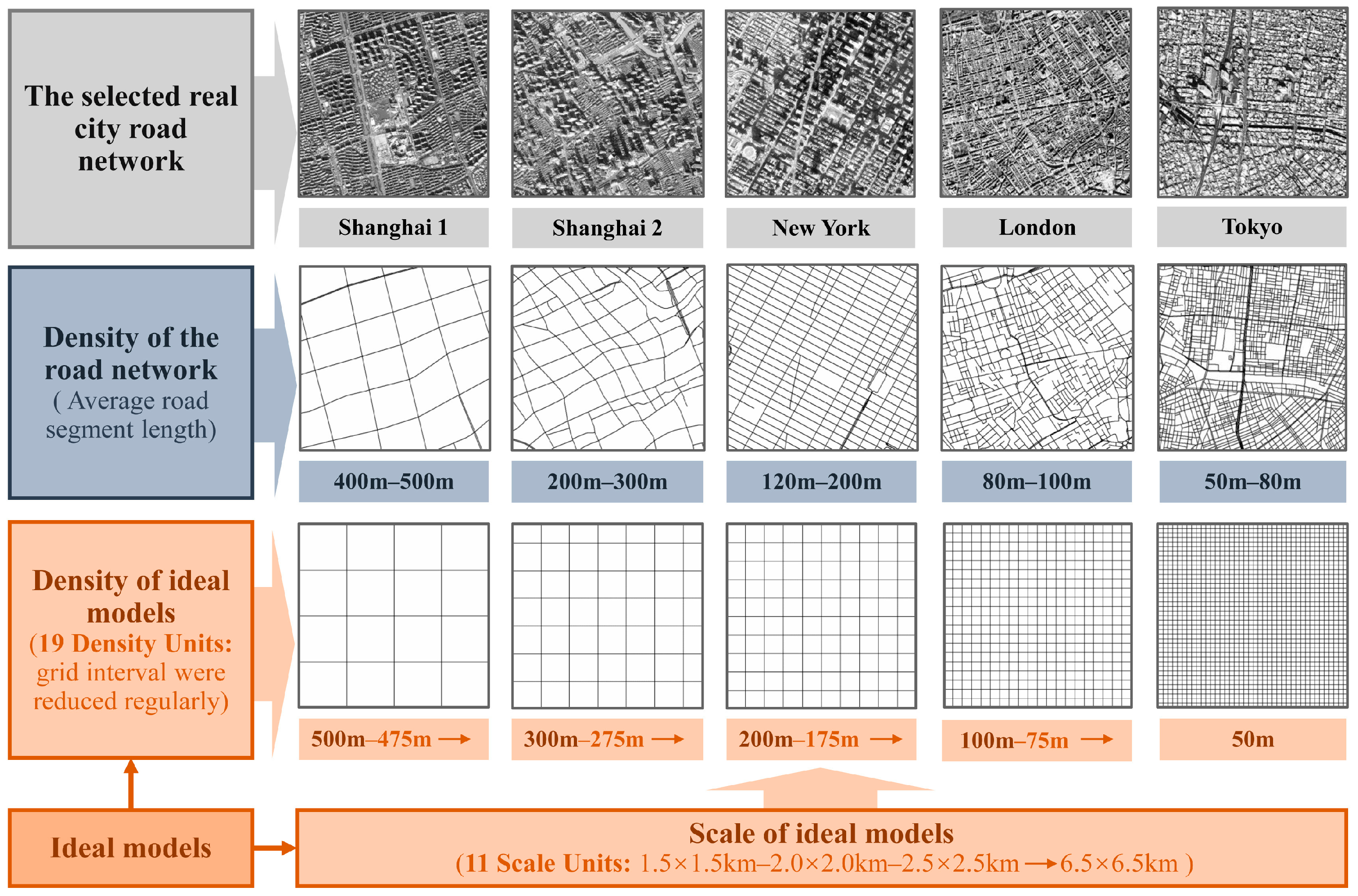
3.1. Designing the Analysis Unit for the Road Network
3.2. Efficiency of the Road Network
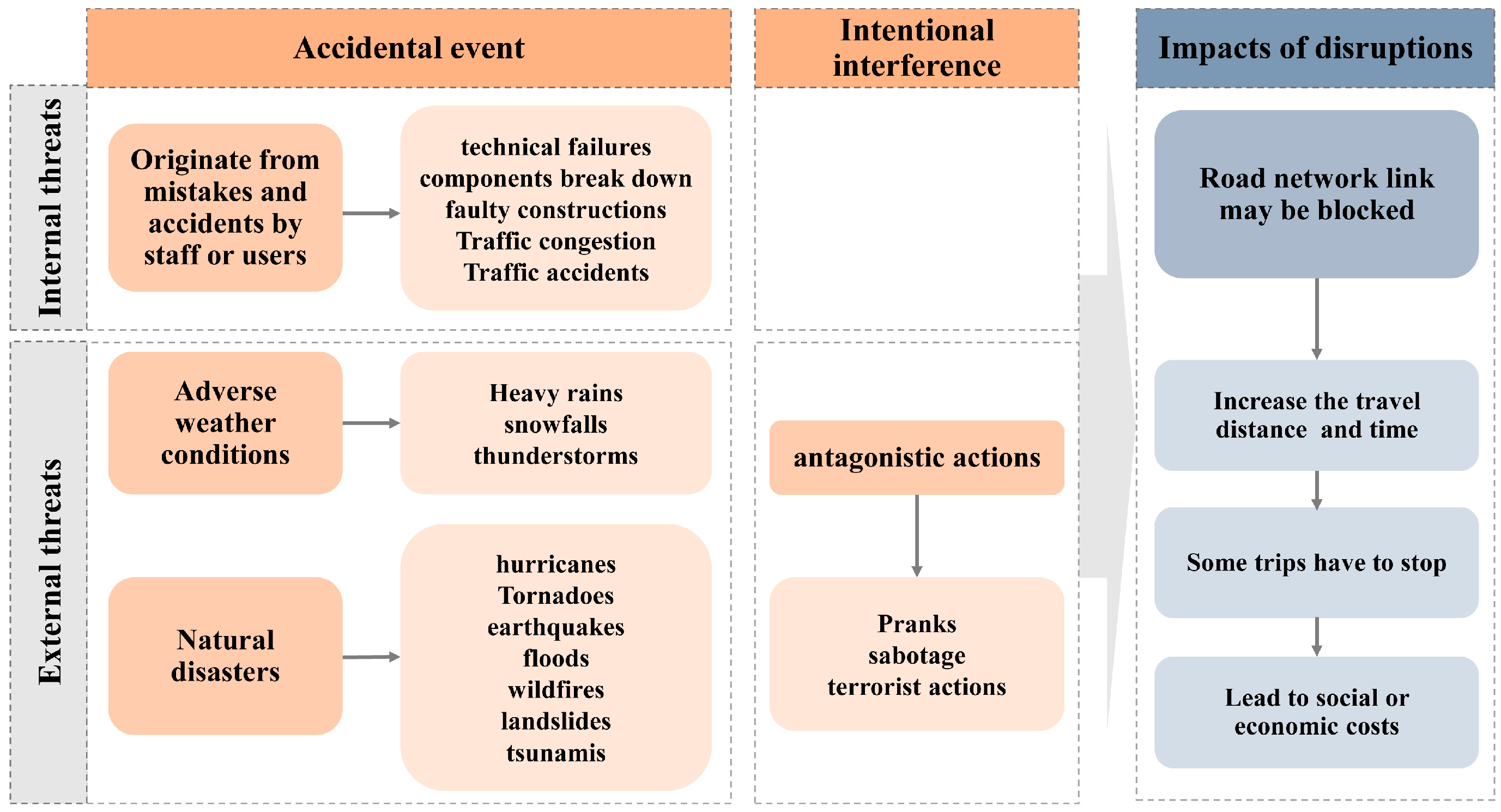
3.3. Designing Two Simulation Scenarios
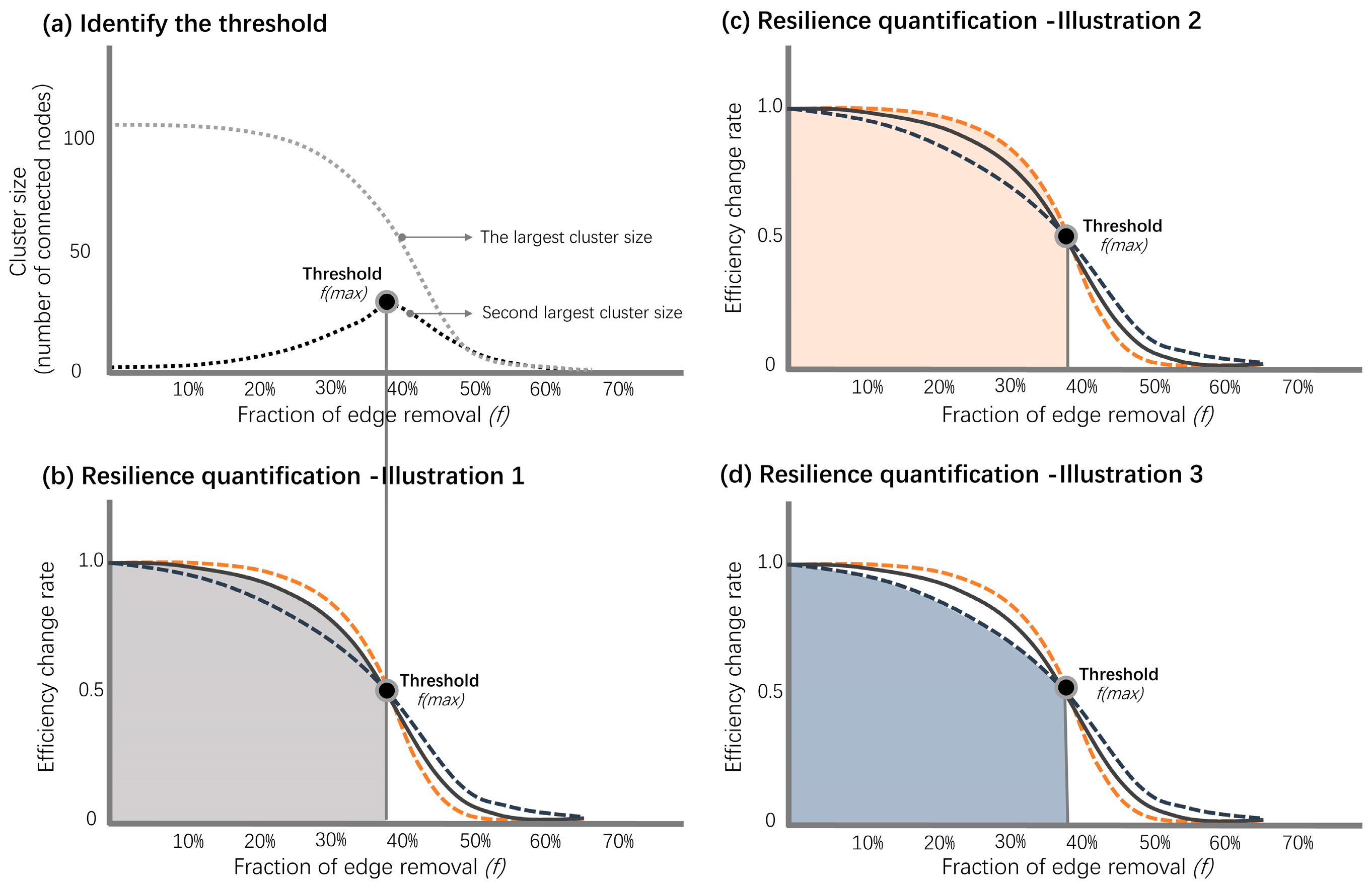
3.4. Measuring the Resilience Level of the Road Network
4. Results
4.1. Resilience Characteristics of Road Networks Under Random Failure Scenarios
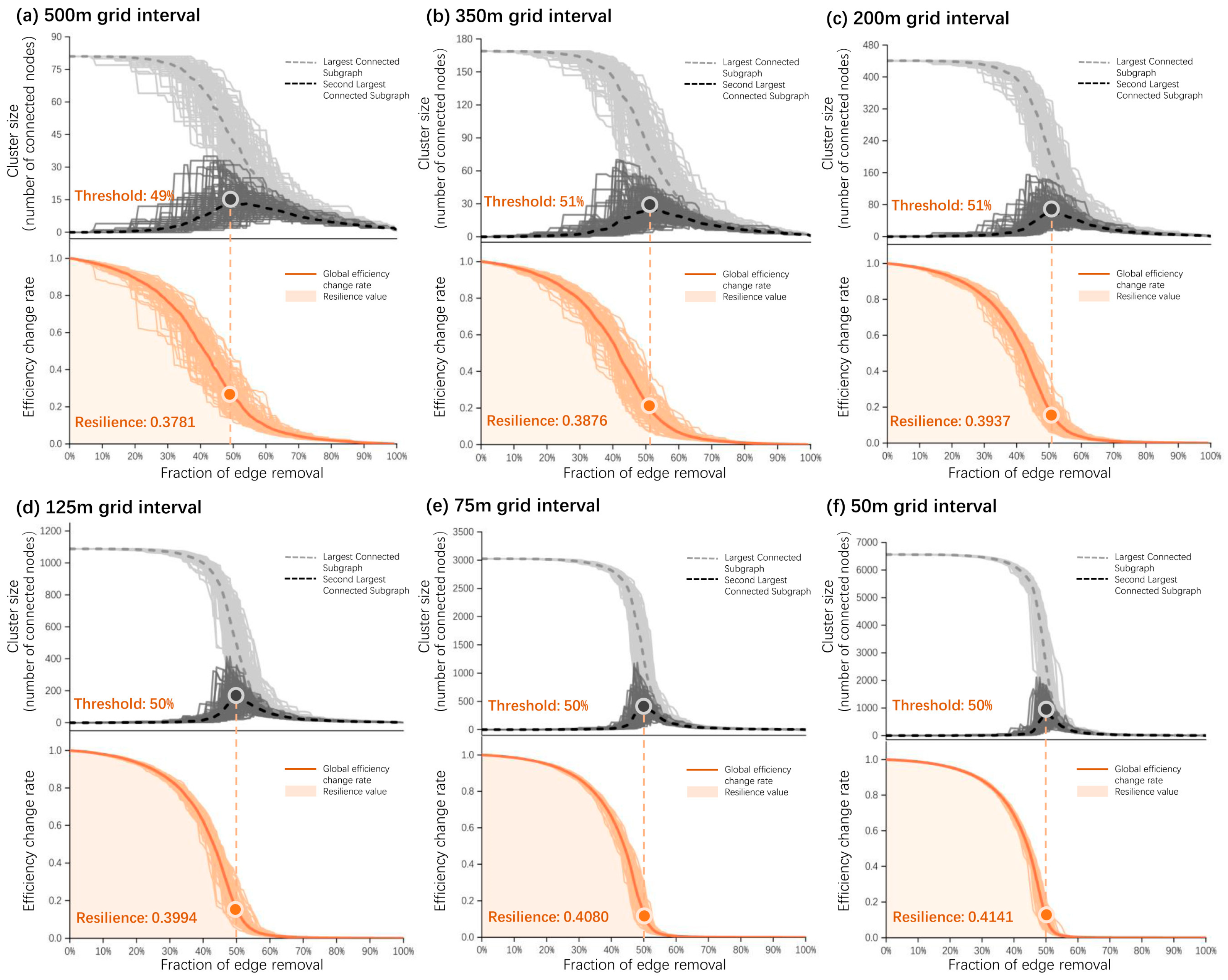
4.1.1. The Overall Trend of Resilience Under Random Failure Scenarios
4.1.2. The Trends in Connected Subgraphs Under Random Failure Scenarios
4.1.3. The Trends in Global Efficiency Under Random Failure Scenarios
4.2. Resilience Characteristics of Road Networks Under Intentional Attack Scenarios
4.2.1. The Overall Trend of Resilience Under Intentional Attack Scenarios
4.2.2. The Trends in Connected Subgraphs Under Intentional Attack Scenarios
4.2.3. The Trends in Global Efficiency Under Intentional Attack Scenarios
4.3. Comparative Analysis of Two Scenarios
4.3.1. Comparative Analysis of Density Distribution Characteristics of Road Network Resilience
4.3.2. Comparative Analysis of the Dynamic Evolution Process of Network Structure
5. Discussion
5.1. Effect of Density on the Resilience of Road Networks
5.2. Implications of Planning Strategies for Enhancing Road Network Resilience
5.3. Limitations and Future Opportunities
6. Conclusions
Author Contributions
Funding
Data Availability Statement
Conflicts of Interest
Appendix A

| Grid Interval | Scale (km) | ||||||||||
|---|---|---|---|---|---|---|---|---|---|---|---|
| 1.5 × 1.5 | 2.0 × 2.0 | 2.5 × 2.5 | 3.0 × 3.0 | 3.5 × 3.5 | 4.0 × 4.0 | 4.5 × 4.5 | 5.0 × 5.0 | 5.5 × 5.5 | 6.0 × 6.0 | 6.5 × 6.5 | |
| 500 m | 16 | 25 | 36 | 49 | 64 | 81 | 100 | 121 | 144 | 169 | 196 |
| 475 m | 25 | 36 | 49 | 64 | 81 | 100 | 121 | 144 | 169 | 196 | 225 |
| 450 m | 25 | 36 | 49 | 64 | 81 | 100 | 121 | 169 | 169 | 225 | 256 |
| 425 m | 25 | 36 | 49 | 81 | 100 | 121 | 144 | 169 | 196 | 256 | 289 |
| 400 m | 25 | 36 | 64 | 81 | 100 | 121 | 169 | 196 | 225 | 256 | 324 |
| 375 m | 25 | 49 | 64 | 81 | 121 | 144 | 169 | 225 | 237 | 289 | 361 |
| 350 m | 36 | 49 | 81 | 100 | 121 | 169 | 196 | 256 | 289 | 361 | 400 |
| 325 m | 36 | 64 | 81 | 121 | 144 | 196 | 225 | 289 | 324 | 400 | 441 |
| 300 m | 36 | 64 | 100 | 121 | 169 | 225 | 256 | 324 | 400 | 441 | 529 |
| 275 m | 49 | 81 | 121 | 144 | 196 | 256 | 324 | 400 | 441 | 529 | 625 |
| 250 m | 49 | 81 | 121 | 169 | 225 | 289 | 361 | 441 | 529 | 625 | 729 |
| 225 m | 64 | 100 | 169 | 225 | 289 | 361 | 441 | 576 | 676 | 784 | 900 |
| 200 m | 64 | 121 | 196 | 256 | 361 | 441 | 576 | 676 | 841 | 961 | 1156 |
| 175 m | 81 | 144 | 256 | 361 | 441 | 576 | 729 | 900 | 1089 | 1296 | 1521 |
| 150 m | 121 | 196 | 324 | 441 | 625 | 784 | 961 | 1225 | 1444 | 1681 | 2025 |
| 125 m | 169 | 289 | 441 | 625 | 841 | 1089 | 1369 | 1681 | 2025 | 2401 | 2809 |
| 100 m | 256 | 441 | 676 | 961 | 1296 | 1681 | 2116 | 2601 | 3136 | 3721 | 4356 |
| 75 m | 441 | 784 | 1225 | 1681 | 2304 | 3025 | 3721 | 4624 | 5625 | 6561 | 7744 |
| 50 m | 961 | 1681 | 2601 | 3721 | 5041 | 6561 | 8281 | 10,201 | 12,321 | 14,641 | 17,161 |
| Grid Interval | Scale (km) | ||||||||||
|---|---|---|---|---|---|---|---|---|---|---|---|
| 1.5 × 1.5 | 2.0 × 2.0 | 2.5 × 2.5 | 3.0 × 3.0 | 3.5 × 3.5 | 4.0 × 4.0 | 4.5 × 4.5 | 5.0 × 5.0 | 5.5 × 5.5 | 6.0 × 6.0 | 6.5 × 6.5 | |
| 500 m | 24 | 40 | 60 | 84 | 112 | 144 | 180 | 220 | 264 | 312 | 364 |
| 475 m | 40 | 60 | 84 | 112 | 144 | 180 | 220 | 264 | 312 | 364 | 420 |
| 450 m | 40 | 60 | 84 | 112 | 144 | 180 | 220 | 312 | 364 | 420 | 480 |
| 425 m | 40 | 60 | 84 | 144 | 180 | 220 | 264 | 312 | 364 | 480 | 544 |
| 400 m | 40 | 60 | 112 | 144 | 180 | 220 | 312 | 364 | 420 | 480 | 612 |
| 375 m | 40 | 84 | 112 | 144 | 220 | 264 | 312 | 420 | 454 | 544 | 684 |
| 350 m | 60 | 84 | 144 | 180 | 220 | 312 | 364 | 480 | 544 | 684 | 760 |
| 325 m | 60 | 112 | 144 | 220 | 264 | 364 | 420 | 544 | 612 | 760 | 840 |
| 300 m | 60 | 112 | 180 | 220 | 312 | 420 | 480 | 612 | 760 | 840 | 1012 |
| 275 m | 84 | 144 | 220 | 264 | 364 | 480 | 612 | 760 | 840 | 1012 | 1200 |
| 250 m | 84 | 144 | 220 | 312 | 420 | 544 | 684 | 840 | 1012 | 1200 | 1404 |
| 225 m | 112 | 180 | 312 | 420 | 544 | 684 | 840 | 1104 | 1300 | 1512 | 1740 |
| 200 m | 112 | 220 | 364 | 480 | 684 | 840 | 1104 | 1300 | 1624 | 1860 | 2244 |
| 175 m | 144 | 264 | 480 | 648 | 840 | 1104 | 1404 | 1740 | 2112 | 2520 | 2964 |
| 150 m | 220 | 364 | 612 | 840 | 1200 | 1512 | 1860 | 2380 | 2812 | 3280 | 3960 |
| 125 m | 312 | 544 | 840 | 1200 | 1624 | 2112 | 2664 | 3280 | 3960 | 4704 | 5512 |
| 100 m | 480 | 840 | 1300 | 1860 | 2520 | 3280 | 4140 | 5100 | 6160 | 7320 | 8580 |
| 75 m | 840 | 1512 | 2380 | 3280 | 4512 | 5940 | 7320 | 9112 | 11,100 | 12,960 | 15,312 |
| 50 m | 1860 | 3280 | 5100 | 7320 | 9940 | 12,960 | 16,380 | 20,200 | 24,420 | 29,040 | 34,060 |
| Grid Interval | Scale (km) | ||||||||||
|---|---|---|---|---|---|---|---|---|---|---|---|
| 1.5 × 1.5 | 2.0 × 2.0 | 2.5 × 2.5 | 3.0 × 3.0 | 3.5 × 3.5 | 4.0 × 4.0 | 4.5 × 4.5 | 5.0 × 5.0 | 5.5 × 5.5 | 6.0 × 6.0 | 6.5 × 6.5 | |
| 500 m | 56 | 72 | 90 | 110 | 132 | 156 | 182 | ||||
| 475 m | 48 | 63 | 80 | 99 | 120 | 143 | 168 | 195 | |||
| 450 m | 48 | 63 | 80 | 99 | 130 | 154 | 180 | 208 | |||
| 425 m | 54 | 70 | 88 | 108 | 130 | 154 | 192 | 221 | |||
| 400 m | 40 | 54 | 70 | 88 | 117 | 140 | 165 | 192 | 234 | ||
| 375 m | 40 | 54 | 77 | 96 | 117 | 150 | 176 | 204 | 247 | ||
| 350 m | 45 | 60 | 77 | 104 | 126 | 160 | 187 | 228 | 260 | ||
| 325 m | 32 | 45 | 66 | 84 | 112 | 135 | 170 | 198 | 240 | 273 | |
| 300 m | 32 | 50 | 66 | 91 | 120 | 144 | 180 | 220 | 252 | 299 | |
| 275 m | 36 | 55 | 72 | 98 | 128 | 162 | 200 | 231 | 276 | 325 | |
| 250 m | 36 | 55 | 78 | 105 | 136 | 171 | 210 | 253 | 300 | 351 | |
| 225 m | 24 | 40 | 65 | 90 | 119 | 152 | 189 | 240 | 286 | 336 | 390 |
| 200 m | 27 | 44 | 70 | 96 | 133 | 168 | 216 | 260 | 319 | 372 | 442 |
| 175 m | 30 | 52 | 80 | 114 | 147 | 192 | 243 | 300 | 363 | 432 | 507 |
| 150 m | 33 | 60 | 90 | 126 | 175 | 224 | 279 | 350 | 418 | 492 | 585 |
| 125 m | 39 | 68 | 105 | 150 | 203 | 264 | 333 | 410 | 495 | 588 | 689 |
| 100 m | 48 | 84 | 130 | 186 | 252 | 328 | 414 | 510 | 616 | 732 | 858 |
| 75 m | 63 | 112 | 175 | 246 | 336 | 440 | 549 | 680 | 825 | 972 | 1144 |
| 50 m | 93 | 164 | 255 | 366 | 497 | 648 | 819 | 1010 | 1221 | 1452 | 1703 |
| Grid Interval | Scale (km) | ||||||||||
|---|---|---|---|---|---|---|---|---|---|---|---|
| 1.5 × 1.5 | 2.0 × 2.0 | 2.5 × 2.5 | 3.0 × 3.0 | 3.5 × 3.5 | 4.0 × 4.0 | 4.5 × 4.5 | 5.0 × 5.0 | 5.5 × 5.5 | 6.0 × 6.0 | 6.5 × 6.5 | |
| 500 m | 0.8115 | 0.8086 | 0.8064 | 0.8046 | 0.8032 | 0.8020 | 0.8011 | ||||
| 475 m | 0.8162 | 0.8119 | 0.8087 | 0.8063 | 0.8045 | 0.8030 | 0.8018 | 0.8008 | |||
| 450 m | 0.8128 | 0.8092 | 0.8066 | 0.8046 | 0.8054 | 0.8033 | 0.8018 | 0.8006 | |||
| 425 m | 0.8163 | 0.8104 | 0.8067 | 0.8042 | 0.8025 | 0.8012 | 0.8018 | 0.8004 | |||
| 400 m | 0.8172 | 0.8108 | 0.8070 | 0.8046 | 0.8045 | 0.8022 | 0.8007 | 0.7996 | 0.7999 | ||
| 375 m | 0.8128 | 0.8086 | 0.8072 | 0.8040 | 0.8020 | 0.8018 | 0.8002 | 0.7990 | 0.7991 | ||
| 350 m | 0.8148 | 0.8078 | 0.8046 | 0.8036 | 0.8013 | 0.8011 | 0.7994 | 0.7996 | 0.7982 | ||
| 325 m | 0.8190 | 0.8096 | 0.8080 | 0.8037 | 0.8029 | 0.8005 | 0.8001 | 0.7986 | 0.7984 | 0.7974 | |
| 300 m | 0.8128 | 0.8094 | 0.8046 | 0.8027 | 0.8018 | 0.7996 | 0.7990 | 0.7986 | 0.7974 | 0.7971 | |
| 275 m | 0.8130 | 0.8094 | 0.8034 | 0.8016 | 0.8004 | 0.7996 | 0.7990 | 0.7974 | 0.7970 | 0.7967 | |
| 250 m | 0.8086 | 0.8046 | 0.8020 | 0.8003 | 0.7990 | 0.7981 | 0.7974 | 0.7968 | 0.7964 | 0.7960 | |
| 225 m | 0.8128 | 0.8066 | 0.8054 | 0.8018 | 0.7997 | 0.7983 | 0.7974 | 0.7974 | 0.7966 | 0.7961 | 0.7957 |
| 200 m | 0.8115 | 0.8046 | 0.8022 | 0.7996 | 0.7988 | 0.7974 | 0.7970 | 0.7962 | 0.7961 | 0.7955 | 0.7954 |
| 175 m | 0.8086 | 0.8032 | 0.8011 | 0.7996 | 0.7974 | 0.7967 | 0.7962 | 0.7959 | 0.7956 | 0.7954 | 0.7952 |
| 150 m | 0.8046 | 0.8011 | 0.7990 | 0.7974 | 0.7970 | 0.7961 | 0.7955 | 0.7954 | 0.7950 | 0.7947 | 0.7947 |
| 125 m | 0.8020 | 0.7990 | 0.7974 | 0.7964 | 0.7957 | 0.7953 | 0.7949 | 0.7947 | 0.7945 | 0.7944 | 0.7942 |
| 100 m | 0.7996 | 0.7974 | 0.7962 | 0.7955 | 0.7950 | 0.7947 | 0.7945 | 0.7943 | 0.7942 | 0.7940 | 0.7940 |
| 75 m | 0.7974 | 0.7961 | 0.7954 | 0.7947 | 0.7945 | 0.7943 | 0.7940 | 0.7940 | 0.7939 | 0.7938 | 0.7938 |
| 50 m | 0.7955 | 0.7947 | 0.7943 | 0.7940 | 0.7939 | 0.7938 | 0.7937 | 0.7937 | 0.7936 | 0.7936 | 0.7936 |
| Grid Interval | Scale (km) | ||||||||||
|---|---|---|---|---|---|---|---|---|---|---|---|
| 1.5 × 1.5 | 2.0 × 2.0 | 2.5 × 2.5 | 3.0 × 3.0 | 3.5 × 3.5 | 4.0 × 4.0 | 4.5 × 4.5 | 5.0 × 5.0 | 5.5 × 5.5 | 6.0 × 6.0 | 6.5 × 6.5 | |
| 500 m | 52% | 49% | 53% | 52% | 51% | 51% | 53% | ||||
| 475 m | 50% | 55% | 50% | 53% | 52% | 51% | 49% | 52% | |||
| 450 m | 52% | 50% | 52% | 50% | 52% | 51% | 52% | 51% | |||
| 425 m | 54% | 51% | 55% | 53% | 53% | 52% | 50% | 52% | |||
| 400 m | 51% | 50% | 52% | 54% | 51% | 49% | 51% | 49% | 50% | ||
| 375 m | 52% | 53% | 51% | 50% | 50% | 51% | 51% | 53% | 52% | ||
| 350 m | 51% | 51% | 52% | 51% | 52% | 52% | 51% | 50% | 51% | ||
| 325 m | 52% | 51% | 51% | 52% | 52% | 52% | 52% | 49% | 52% | 51% | |
| 300 m | 52% | 50% | 52% | 52% | 52% | 51% | 53% | 51% | 50% | 51% | |
| 275 m | 53% | 52% | 48% | 52% | 52% | 52% | 53% | 51% | 52% | 50% | |
| 250 m | 55% | 53% | 51% | 49% | 53% | 50% | 51% | 50% | 52% | 52% | |
| 225 m | 50% | 53% | 52% | 54% | 51% | 51% | 50% | 51% | 51% | 49% | 50% |
| 200 m | 53% | 53% | 50% | 51% | 52% | 51% | 52% | 51% | 50% | 50% | 51% |
| 175 m | 50% | 51% | 49% | 52% | 52% | 50% | 53% | 51% | 50% | 51% | 51% |
| 150 m | 50% | 50% | 52% | 50% | 52% | 52% | 51% | 51% | 50% | 51% | 50% |
| 125 m | 50% | 50% | 51% | 49% | 51% | 50% | 50% | 50% | 51% | 51% | 51% |
| 100 m | 51% | 51% | 50% | 52% | 50% | 50% | 52% | 51% | 51% | 50% | 50% |
| 75 m | 52% | 52% | 50% | 51% | 51% | 50% | 50% | 50% | 50% | 51% | 50% |
| 50 m | 50% | 51% | 50% | 51% | 51% | 50% | 51% | 50% | 50% | 50% | 50% |
| Grid Interval | Scale (km) | ||||||||||
|---|---|---|---|---|---|---|---|---|---|---|---|
| 1.5 × 1.5 | 2.0 × 2.0 | 2.5 × 2.5 | 3.0 × 3.0 | 3.5 × 3.5 | 4.0 × 4.0 | 4.5 × 4.5 | 5.0 × 5.0 | 5.5 × 5.5 | 6.0 × 6.0 | 6.5 × 6.5 | |
| 500 m | 8% | 7% | 6% | 6% | 6% | 13% | 7% | ||||
| 475 m | 8% | 7% | 6% | 6% | 6% | 13% | 7% | 8% | |||
| 450 m | 8% | 7% | 6% | 6% | 13% | 7% | 8% | 8% | |||
| 425 m | 7% | 6% | 6% | 6% | 13% | 7% | 8% | 9% | |||
| 400 m | 8% | 7% | 6% | 6% | 13% | 7% | 8% | 8% | 9% | ||
| 375 m | 8% | 7% | 6% | 6% | 13% | 8% | 8% | 9% | 9% | ||
| 350 m | 7% | 6% | 6% | 13% | 7% | 8% | 9% | 9% | 10% | ||
| 325 m | 8% | 7% | 6% | 6% | 7% | 8% | 9% | 9% | 10% | 10% | |
| 300 m | 8% | 6% | 6% | 13% | 8% | 8% | 9% | 10% | 10% | 11% | |
| 275 m | 7% | 6% | 6% | 7% | 8% | 9% | 10% | 10% | 11% | 12% | |
| 250 m | 7% | 6% | 13% | 8% | 9% | 9% | 10% | 11% | 12% | 13% | |
| 225 m | 8% | 6% | 13% | 8% | 9% | 9% | 10% | 12% | 12% | 12% | 14% |
| 200 m | 7% | 6% | 7% | 8% | 9% | 10% | 12% | 12% | 14% | 14% | 16% |
| 175 m | 6% | 13% | 8% | 9% | 10% | 12% | 13% | 14% | 15% | 16% | 17% |
| 150 m | 6% | 8% | 9% | 10% | 12% | 12% | 14% | 16% | 17% | 18% | 19% |
| 125 m | 13% | 9% | 10% | 12% | 14% | 15% | 14% | 18% | 19% | 19% | 20% |
| 100 m | 8% | 10% | 12% | 14% | 16% | 18% | 19% | 20% | 22% | 23% | 24% |
| 75 m | 10% | 12% | 16% | 18% | 18% | 21% | 23% | 25% | 28% | 29% | 31% |
| 50 m | 14% | 18% | 20% | 23% | 26% | 29% | 31% | 33% | 36% | 39% | 41% |
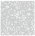
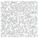
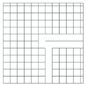
| Network Structure 1 | Network Structure 2 | Network Structure 3 | Network Structure 4 | Network Structure 5 |
 |  | 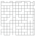 |  |  |
| f = 5% | f = 10% | f = 15% | f = 20% | f = 25% |
| Network Structure 6 | Network Structure 7 | Network Structure 8 | Network Structure 9 | Network Structure 10 |
 |  |  | 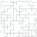 |  |
| f = 30% | f = 35% | f = 40% | f = 45% | Threshold f = 50% |
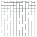
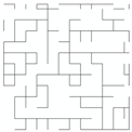
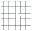
| Network Structure 1 | Network Structure 2 | Network Structure 3 | Network Structure 4 | Network Structure 5 |
 |  |  |  | 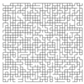 |
| f = 5% | f = 10% | f = 15% | f = 20% | f = 25% |
| Network Structure 6 | Network Structure 7 | Network Structure 8 | Network Structure 9 | Network Structure 10 |
 |  |  | 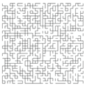 |  |
| f = 30% | f = 35% | f = 40% | f = 45% | Threshold f = 53% |
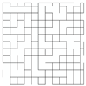
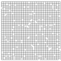
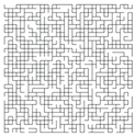
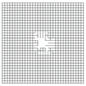
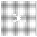
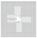
| Network Structure 1 | Network Structure 2 | Network Structure 3 | Network Structure 4 | Network Structure 5 |
 | 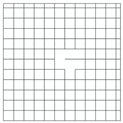 |  |  |  |
| f = 1% | f = 2% | f = 3% | f = 4% | f = 5% |
| Network Structure 6 | Network Structure 7 | Network Structure 8 | Network Structure 9 | Network Structure 10 |
 |  |  |  |  |
| f = 6% | f = 7% | f = 8% | f = 9% | f = 10% |
| Network Structure 11 | Network Structure 12 | Network Structure 13 | Network Structure 14 | Network Structure 15 |
 |  |  |  |  |
| f = 11% | f = 12% | Threshold f = 13% | f = 14% | f = 15% |
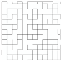
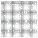
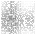
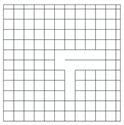
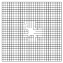
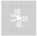
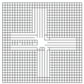
| Network Structure 1 | Network Structure 2 | Network Structure 3 | Network Structure 4 | Network Structure 5 |
 |  |  |  |  |
| f = 1% | f = 2% | f = 3% | f = 4% | f = 5% |
| Network Structure 6 | Network Structure 7 | Network Structure 8 | Network Structure 9 | Network Structure 10 |
 |  |  |  |  |
| f = 6% | Threshold f = 7% | f = 8% | f = 9% | f = 10% |
| Network Structure 11 | Network Structure 12 | Network Structure 13 | Network Structure 14 | Network Structure 15 |
 |  |  |  |  |
| f = 11% | f = 12% | f = 13% | f = 14% | f = 15% |
| Network Structure 1 | Network Structure 2 | Network Structure 3 | Network Structure 4 | Network Structure 5 |
 |  |  |  |  |
| f = 1% | f = 2% | f = 3% | f = 4% | f = 5% |
| Network Structure 6 | Network Structure 7 | Network Structure 8 | Network Structure 9 | Network Structure 10 |
 |  | 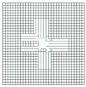 | 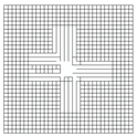 |  |
| f = 6% | f = 7% | f = 8% | f = 9% | f = 10% |
| Network Structure 11 | Network Structure 12 | Network Structure 13 | Network Structure 14 | Network Structure 15 |
 |  | 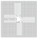 | 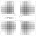 |  |
| f = 11% | f = 12% | f = 13% | f = 14% | Threshold f = 15% |
| Source | Sum of Squares | Degrees of Freedom | Mean Square | F | Significance |
|---|---|---|---|---|---|
| Between | 92,644,663.14 | 10 | 9,264,466.314 | 1.952 | 0.040 |
| Within | 939,599,202.3 | 198 | 4,745,450.517 | ||
| Total | 103,224,865 | 208 |
| Source | Sum of Squares | Degrees of Freedom | Mean Square | F | Significance |
|---|---|---|---|---|---|
| Between | 637,684,750.7 | 18 | 35,426,930.60 | 17.060 | 0.000 |
| Within | 394,559,114.7 | 190 | 2,076,626.920 | ||
| Total | 1,032,243,865 | 208 |
| Source | Sum of Squares | Degrees of Freedom | Mean Square | F | Significance |
|---|---|---|---|---|---|
| Between | 361,359,539.1 | 10 | 36,135,953.91 | 1.937 | 0.042 |
| Within | 3,694,146,164 | 198 | 18,657,303.83 | ||
| Total | 4,055,505,703 | 208 |
| Source | Sum of Squares | Degrees of Freedom | Mean Square | F | Significance |
|---|---|---|---|---|---|
| Between | 2,500,238,360 | 10 | 138,902,131.1 | 16.969 | 0.000 |
| Within | 1,555,267,343 | 198 | 8,185,617.596 | ||
| Total | 4,055,505,703 | 208 |
| Source | Sum of Squares | Degrees of Freedom | Mean Square | F | Significance |
|---|---|---|---|---|---|
| Between | 0.002 | 10 | 0.000 | 2.258 | 0.017 |
| Within | 0.013 | 175 | 0.000 | ||
| Total | 0.015 | 185 |
| Source | Sum of Squares | Degrees of Freedom | Mean Square | F | Significance |
|---|---|---|---|---|---|
| Between | 0.054 | 10 | 0.005 | 1.954 | 0.041 |
| Within | 0.480 | 175 | 0.003 | ||
| Total | 0.534 | 185 |
References
- Ahern, J. From fail-safe to safe-to-fail: Sustainability and resilience in the new urban world. Landsc. Urban Plan. 2011, 100, 341–343. [Google Scholar] [CrossRef]
- Lhomme, S.; Serre, D.; Diab, Y.; Laganier, R. Analyzing resilience of urban networks: A preliminary step towards more flood resilient cities. Nat. Hazards Earth Syst. Sci. 2013, 13, 221–230. [Google Scholar] [CrossRef]
- Allan, P.; Bryant, M.; Wirsching, C.; Garcia, D.; Teresa Rodriguez, M. The Influence of Urban Morphology on the Resilience of Cities Following an Earthquake. J. Urban Des. 2013, 18, 242–262. [Google Scholar] [CrossRef]
- León, J.; March, A. Urban morphology as a tool for supporting tsunami rapid resilience: A case study of Talcahuano, Chile. Habitat Int. 2014, 43, 250–262. [Google Scholar] [CrossRef]
- Sharifi, A. Urban form resilience: A meso-scale analysis. Cities 2019, 93, 238–252. [Google Scholar] [CrossRef]
- Sharifi, A. Resilient urban forms: A macro-scale analysis. Cities 2019, 85, 1–14. [Google Scholar] [CrossRef]
- Dong, S.; Mostafizi, A.; Wang, H.; Gao, J.; Li, X. Measuring the Topological Robustness of Transportation Networks to Disaster-Induced Failures: A Percolation Approach. J. Infrastruct. Syst. 2020, 26, 04020009. [Google Scholar] [CrossRef]
- Cavallaro, M.; Asprone, D.; Latora, V.; Manfredi, G.; Nicosia, V. Assessment of Urban Ecosystem Resilience through Hybrid Social–Physical Complex Networks. Comput. Civ. Infrastruct. Eng. 2014, 29, 608–625. [Google Scholar] [CrossRef]
- Batty, M. Resilient cities, networks, and disruption. Environ. Plan. B Plan. Des. 2013, 40, 571–573. [Google Scholar] [CrossRef]
- Sharifi, A. Resilient urban forms: A review of literature on streets and street networks. Build. Environ. 2019, 147, 171–187. [Google Scholar] [CrossRef]
- Zare, N.; Macioszek, E.; Granà, A.; Giuffrè, T. Blending Efficiency and Resilience in the Performance Assessment of Urban Intersections: A Novel Heuristic Informed by Literature Review. Sustainability 2024, 16, 2450. [Google Scholar] [CrossRef]
- Dong, S.; Esmalian, A.; Farahmand, H.; Mostafavi, A. An integrated physical-social analysis of disrupted access to critical facilities and community service-loss tolerance in urban flooding. Comput. Environ. Urban Syst. 2020, 80, 101443. [Google Scholar] [CrossRef]
- Hao, H.; Wang, Y. Disentangling relations between urban form and urban accessibility for resilience to extreme weather and climate events. Landsc. Urban Plan. 2022, 220, 104352. [Google Scholar] [CrossRef]
- Mattsson, L.-G.; Jenelius, E. Vulnerability and resilience of transport systems—A discussion of recent research. Transp. Res. Part A 2015, 81, 16–34. [Google Scholar] [CrossRef]
- Ewing, R.; Cervero, R. Travel and the Built Environment: A meta-analysis. J. Am. Plan. Assoc. 2010, 76, 265–294. [Google Scholar] [CrossRef]
- Shirazi, M.R. Compact Urban Form: Neighbouring and Social Activity. Sustainability 2020, 12, 1987. [Google Scholar] [CrossRef]
- Larco, N. Sustainable urban design—A (draft) framework. J. Urban Des. 2015, 21, 1–29. [Google Scholar] [CrossRef]
- Lehmann, S. Sustainable urbanism: Towards a framework for quality and optimal density? Future Cities Environ. 2016, 2, 8. [Google Scholar] [CrossRef]
- Bourdic, L.; Salat, S.; Nowacki, C. Assessing cities: A new system of cross-scale spatial indicators. Build. Res. Inf. 2012, 40, 592–605. [Google Scholar] [CrossRef]
- Feliciotti, A.; Romice, O.; Porta, S. Design for Change: Five Proxies for Resilience in the Urban Form. Open House Int. 2016, 41, 23–30. [Google Scholar] [CrossRef]
- Salat, S. Cities and Forms: On Sustainable Urbanism; China Architecture & Building Press: Beijing, China, 2012. [Google Scholar]
- Salat, S. A systemic approach of urban resilience: Power laws and urban growth patterns. Int. J. Urban Sustain. Dev. 2017, 9, 107–135. [Google Scholar] [CrossRef]
- Carpenter, A. Resilience in the social and physical realms: Lessons from the Gulf Coast. Int. J. Disaster Risk Reduct. 2015, 14, 290–301. [Google Scholar] [CrossRef]
- Yan, W.; Lu, J.; Li, Z.; Shen, Y. Implications of Measuring Resilience of Urban Street Networks: Comparative Study of Five Global Cities. Urban Plan. Int. 2021, 36, 13. (In Chinese) [Google Scholar] [CrossRef]
- Ostadtaghizadeh, A.; Ardalan, A.; Paton, D.; Jabbari, H.; Khankeh, H.R. Community disaster resilience: A systematic review on assessment models and tools. PLoS Curr. 2015, 7, ecurrents-dis. [Google Scholar] [CrossRef]
- Ribeiro, P.J.G.; Pena Jardim Gonçalves, L.A. Urban resilience: A conceptual framework. Sustain. Cities Soc. 2019, 50, 101625. [Google Scholar] [CrossRef]
- Meerow, S.; Newell, J.P.; Stults, M. Defining urban resilience: A review. Landsc. Urban Plan. 2016, 147, 38–49. [Google Scholar] [CrossRef]
- Muñoz-Erickson, T.A.; Meerow, S.; Hobbins, R.; Cook, E.; Iwaniec, D.M.; Berbés-Blázquez, M.; Grimm, N.B.; Barnett, A.; Cordero, J.; Gim, C.; et al. Beyond bouncing back? Comparing and contesting urban resilience frames in US and Latin American contexts. Landsc. Urban Plan. 2021, 214, 104173. [Google Scholar] [CrossRef]
- Carpenter, S.R.; Westley, F.; Turner, M.G. Surrogates for Resilience of Social–Ecological Systems. Ecosystems 2005, 8, 941–944. [Google Scholar] [CrossRef]
- Godschalk, D.R. Urban Hazard Mitigation: Creating Resilient Cities. Nat. Hazards Rev. 2003, 4, 136–143. [Google Scholar] [CrossRef]
- Gonçalves, L.A.P.J.; Ribeiro, P.J.G. Resilience of urban transportation systems. Concept, characteristics, and methods. J. Transp. Geogr. 2020, 85, 102727. [Google Scholar] [CrossRef]
- Lu, P.; Stead, D. Understanding the notion of resilience in spatial planning: A case study of Rotterdam, The Netherlands. Cities 2013, 35, 200–212. [Google Scholar] [CrossRef]
- McDaniels, T.; Chang, S.; Cole, D.; Mikawoz, J.; Longstaff, H. Fostering resilience to extreme events within infrastructure systems: Characterizing decision contexts for mitigation and adaptation. Glob. Environ. Change 2008, 18, 310–318. [Google Scholar] [CrossRef]
- Tang, J.; Han, S.; Wang, J.; He, B.; Peng, J. A Comparative Analysis of Performance-Based Resilience Metrics via a Quantitative-Qualitative Combined Approach: Are We Measuring the Same Thing? Int. J. Disaster Risk Sci. 2023, 14, 736–750. [Google Scholar] [CrossRef]
- Bruneau, M.; Reinhorn, A. Exploring the Concept of Seismic Resilience for Acute Care Facilities. Earthq. Spectra 2007, 23, 41–62. [Google Scholar] [CrossRef]
- Cimellaro, G.P.; Reinhorn, A.M.; Bruneau, M. Framework for analytical quantification of disaster resilience. Eng. Struct. 2010, 32, 3639–3649. [Google Scholar] [CrossRef]
- Cutter, S.L.; Barnes, L.; Berry, M.; Burton, C.; Evans, E.; Tate, E.; Webb, J. A place-based model for understanding community resilience to natural disasters. Glob. Environ. Change 2008, 18, 598–606. [Google Scholar] [CrossRef]
- Ouyang, M.; Dueñas-Osorio, L.; Min, X. A three-stage resilience analysis framework for urban infrastructure systems. Struct. Saf. 2012, 36–37, 23–31. [Google Scholar] [CrossRef]
- Iyer, S.; Killingback, T.; Sundaram, B.; Wang, Z. Attack Robustness and Centrality of Complex Networks. PLoS ONE 2013, 8, e59613. [Google Scholar] [CrossRef]
- Wang, J. Resilience of Self-Organised and Top-Down Planned Cities—A Case Study on London and Beijing Street Networks. PLoS ONE 2015, 10, e0141736. [Google Scholar] [CrossRef]
- Crucitti, P.; Latora, V.; Marchiori, M.; Rapisarda, A. Error and attack tolerance of complex networks. Phys. A Stat. Mech. Its Appl. 2004, 340, 388–394. [Google Scholar] [CrossRef]
- Sakakibara, H.; Kajitani, Y.; Okada, N. Road Network Robustness for Avoiding Functional Isolation in Disasters. J. Transp. Eng. 2004, 130, 560–567. [Google Scholar] [CrossRef]
- Li, Z.; Yan, W. Service flow changes in multilayer networks: A framework for measuring urban disaster resilience based on availability to critical facilities. Landsc. Urban Plan. 2023, 244, 104996. [Google Scholar] [CrossRef]
- Newman, M.E.J. Networks: An Introduction; Oxford University Press: Oxford, UK, 2010. [Google Scholar]
- Mehaffy, M.; Porta, S.; Rofè, Y.; Salingaros, N. Urban nuclei and the geometry of streets: The ‘emergent neighborhoods’ model. Urban Des. Int. 2010, 15, 22–46. [Google Scholar] [CrossRef]
- Sharifi, A.; Yamagata, Y. Resilient Urban Planning: Major Principles and Criteria. Energy Procedia 2014, 61, 1491–1495. [Google Scholar] [CrossRef]
- Xu, X.; Chen, A.; Xu, G.; Yang, C.; Lam, W.H. Enhancing network resilience by adding redundancy to road networks. Transp. Res. Part E Logist. Transp. Rev. 2021, 154, 102448. [Google Scholar] [CrossRef]
- Boeing, G. OSMnx: New methods for acquiring, constructing, analyzing, and visualizing complex street networks. Comput. Environ. Urban Syst. 2017, 65, 126–139. [Google Scholar] [CrossRef]
- Marshall, S. Streets and Patterns; Spon Press: New York, NY, USA, 2005. [Google Scholar]
- Porta, S.; Romice, O.; Maxwell, J.A.; Russell, P.; Baird, D. Alterations in scale: Patterns of change in main street networks across time and space. Urban Stud. 2014, 51, 3383–3400. [Google Scholar] [CrossRef]
- Duan, Y.; Lu, F. Structural robustness of city road networks based on community. Comput. Environ. Urban Syst. 2013, 41, 75–87. [Google Scholar] [CrossRef]
- Porta, S.; Crucitti, P.; Latora, V. The Network Analysis of Urban Streets: A Dual Approach. Phys. A Stat. Mech. Its Appl. 2006, 369, 853–866. [Google Scholar] [CrossRef]
- Latora, V.; Marchiori, M. Efficient Behavior of Small-World Networks. Phys. Rev. Lett. 2001, 87, 198701. [Google Scholar] [CrossRef]
- Li, Z. Evolution Characteristics of Urban Resilience and Spatial Regulation Strategies from the Perspective of Urban Complex System: A Case Study of Shanghai; Tongji University: Shanghai, China, 2022; p. 58. (In Chinese) [Google Scholar]
- Li, D.; Fu, B.; Wang, Y.; Lu, G.; Berezin, Y.; Stanley, H.E.; Havlin, S. Percolation transition in dynamical traffic network with evolving critical bottlenecks. Proc. Natl. Acad. Sci. USA 2015, 112, 669–672. [Google Scholar] [CrossRef] [PubMed]
- Li, M.; Liu, R.-R.; Lü, L.; Hu, M.-B.; Xu, S.; Zhang, Y.-C. Percolation on complex networks: Theory and application. Phys. Rep. 2021, 907, 1–68. [Google Scholar] [CrossRef]
- Masucci, A.P.; Molinero, C. Robustness and closeness centrality for self-organized and planned cities. Eur. Phys. J. B 2016, 89, 53. [Google Scholar] [CrossRef]
- Wang, W.; Yang, S.; Stanley, H.E.; Gao, J. Local floods induce large-scale abrupt failures of road networks. Nat. Commun. 2019, 10, 2114. [Google Scholar] [CrossRef]
- Deng, Y.; Blöte, H.W.J. Monte Carlo study of the site-percolation model in two and three dimensions. Phys. Rev. E 2005, 72 Pt 2, 016126. [Google Scholar] [CrossRef]
- Newman, M.E.J.; Jensen, I.; Ziff, R.M. Percolation and epidemics in a two-dimensional small world. Phys. Rev. E 2002, 65 Pt 1, 021904. [Google Scholar] [CrossRef]
- Zhang, X.; Miller-Hooks, E.; Denny, K. Assessing the role of network topology in transportation network resilience. J. Transp. Geogr. 2015, 46, 35–45. [Google Scholar] [CrossRef]
- Lak, A.; Hasankhan, F.; Garakani, S.A. Principles in practice: Toward a conceptual framework for resilient urban design. J. Environ. Plan. Manag. 2020, 63, 2194–2226. [Google Scholar] [CrossRef]
- Dastjerdi, M.S.; Lak, A.; Ghaffari, A.; Sharifi, A. A conceptual framework for resilient place assessment based on spatial resilience approach: An integrative review. Urban Clim. 2021, 36, 100794. [Google Scholar] [CrossRef]
- Liao, K.-H. A Theory on Urban Resilience to Floods—A Basis for Alternative Planning Practices. Ecol. Soc. 2012, 17, 388–395. [Google Scholar] [CrossRef]
- Dempsey, N.; Brown, C.; Bramley, G. The key to sustainable urban development in UK cities? The influence of density on social sustainability. Prog. Plan. 2012, 77, 89–141. [Google Scholar] [CrossRef]
- Scudellari, J.; Staricco, L.; Brovarone, E.V. Implementing the Supermanzana approach in Barcelona. Critical issues at local and urban level. J. Urban Des. 2019, 25, 675–696. [Google Scholar] [CrossRef]
- Siksna, A. The evolution of block size and form in North American and Australian city centres. Urban Morphol. 1996, 1, 19–33. [Google Scholar] [CrossRef]
- Kan, H.Y.; Forsyth, A.; Rowe, P. Redesigning China’s superblock neighbourhoods: Policies, opportunities and challenges. J. Urban Des. 2017, 22, 757–777. [Google Scholar] [CrossRef]


| Grid Interval | Scale (km) | ||||||||||
|---|---|---|---|---|---|---|---|---|---|---|---|
| 1.5 × 1.5 | 2.0 × 2.0 | 2.5 × 2.5 | 3.0 × 3.0 | 3.5 × 3.5 | 4.0 × 4.0 | 4.5 × 4.5 | 5.0 × 5.0 | 5.5 × 5.5 | 6.0 × 6.0 | 6.5 × 6.5 | |
| 500 m | 0.3853 | 0.3781 | 0.3881 | 0.3882 | 0.3850 | 0.3868 | 0.3911 | ||||
| 475 m | 0.3810 | 0.3941 | 0.3817 | 0.3925 | 0.3884 | 0.3868 | 0.3831 | 0.3878 | |||
| 450 m | 0.3864 | 0.3825 | 0.3856 | 0.3814 | 0.3901 | 0.3903 | 0.3896 | 0.3872 | |||
| 425 m | 0.3951 | 0.3866 | 0.3920 | 0.3898 | 0.3908 | 0.3904 | 0.3866 | 0.3918 | |||
| 400 m | 0.3828 | 0.3822 | 0.3863 | 0.3913 | 0.3889 | 0.3829 | 0.3878 | 0.3836 | 0.3886 | ||
| 375 m | 0.3846 | 0.3875 | 0.3878 | 0.3846 | 0.3836 | 0.3881 | 0.3894 | 0.3952 | 0.3929 | ||
| 350 m | 0.3876 | 0.3847 | 0.3876 | 0.3876 | 0.3892 | 0.3915 | 0.3897 | 0.3892 | 0.3929 | ||
| 325 m | 0.3896 | 0.3837 | 0.3863 | 0.3895 | 0.3886 | 0.3895 | 0.3923 | 0.3864 | 0.3941 | 0.3932 | |
| 300 m | 0.3894 | 0.3820 | 0.3879 | 0.3907 | 0.3894 | 0.3904 | 0.3952 | 0.3910 | 0.3904 | 0.3932 | |
| 275 m | 0.3917 | 0.3881 | 0.3771 | 0.3891 | 0.3886 | 0.3956 | 0.3963 | 0.3915 | 0.3959 | 0.3940 | |
| 250 m | 0.3915 | 0.3906 | 0.3857 | 0.3825 | 0.3921 | 0.3909 | 0.3927 | 0.3934 | 0.3953 | 0.3972 | |
| 225 m | 0.3801 | 0.388 | 0.3904 | 0.3947 | 0.3893 | 0.3920 | 0.3925 | 0.3956 | 0.3966 | 0.3952 | 0.3969 |
| 200 m | 0.3906 | 0.3875 | 0.3853 | 0.3883 | 0.3944 | 0.3937 | 0.3964 | 0.3956 | 0.3972 | 0.3970 | 0.4024 |
| 175 m | 0.3836 | 0.3891 | 0.3849 | 0.3943 | 0.3931 | 0.3941 | 0.4002 | 0.3982 | 0.3996 | 0.4045 | 0.4042 |
| 150 m | 0.3812 | 0.3862 | 0.3939 | 0.3928 | 0.3967 | 0.3993 | 0.4001 | 0.4019 | 0.4011 | 0.4045 | 0.4047 |
| 125 m | 0.3834 | 0.3867 | 0.3915 | 0.3918 | 0.3978 | 0.3994 | 0.4012 | 0.4026 | 0.4067 | 0.4075 | 0.4092 |
| 100 m | 0.3894 | 0.3913 | 0.3948 | 0.4001 | 0.4015 | 0.4037 | 0.4069 | 0.4082 | 0.4092 | 0.4099 | 0.4111 |
| 75 m | 0.3955 | 0.4010 | 0.4012 | 0.4043 | 0.4074 | 0.4080 | 0.4092 | 0.4111 | 0.4123 | 0.4156 | 0.4153 |
| 50 m | 0.3968 | 0.4048 | 0.4070 | 0.4095 | 0.4133 | 0.4141 | 0.4156 | 0.4172 | 0.4197 | 0.4204 | 0.4219 |
| Grid Interval | Scale (km) | ||||||||||
|---|---|---|---|---|---|---|---|---|---|---|---|
| 1.5 × 1.5 | 2.0 × 2.0 | 2.5 × 2.5 | 3.0 × 3.0 | 3.5 × 3.5 | 4.0 × 4.0 | 4.5 × 4.5 | 5.0 × 5.0 | 5.5 × 5.5 | 6.0 × 6.0 | 6.5 × 6.5 | |
| 500 m | 0.0733 | 0.0637 | 0.0545 | 0.0554 | 0.0551 | 0.0842 | 0.0642 | ||||
| 475 m | 0.0738 | 0.0639 | 0.0546 | 0.0555 | 0.0552 | 0.0836 | 0.0643 | 0.0715 | |||
| 450 m | 0.0735 | 0.0638 | 0.0545 | 0.0554 | 0.0829 | 0.0643 | 0.0716 | 0.0696 | |||
| 425 m | 0.0641 | 0.0547 | 0.0555 | 0.0552 | 0.0839 | 0.0642 | 0.0697 | 0.0810 | |||
| 400 m | 0.0739 | 0.0639 | 0.0545 | 0.0554 | 0.0831 | 0.0643 | 0.0715 | 0.0695 | 0.0780 | ||
| 375 m | 0.0735 | 0.0637 | 0.0555 | 0.0552 | 0.0842 | 0.0716 | 0.0696 | 0.0808 | 0.0797 | ||
| 350 m | 0.0640 | 0.0546 | 0.0554 | 0.0834 | 0.0642 | 0.0697 | 0.0809 | 0.0797 | 0.0868 | ||
| 325 m | 0.0740 | 0.0638 | 0.0555 | 0.0551 | 0.0643 | 0.0715 | 0.0809 | 0.0779 | 0.0868 | 0.0887 | |
| 300 m | 0.0735 | 0.0547 | 0.0554 | 0.0838 | 0.0716 | 0.0695 | 0.0779 | 0.0868 | 0.0887 | 0.0954 | |
| 275 m | 0.0640 | 0.0555 | 0.0551 | 0.0643 | 0.0696 | 0.0780 | 0.0869 | 0.0887 | 0.0954 | 0.1039 | |
| 250 m | 0.0637 | 0.0554 | 0.0842 | 0.0715 | 0.0808 | 0.0796 | 0.0887 | 0.0953 | 0.1038 | 0.1122 | |
| 225 m | 0.0735 | 0.0545 | 0.0829 | 0.0716 | 0.0809 | 0.0796 | 0.0887 | 0.1027 | 0.1042 | 0.1063 | 0.1213 |
| 200 m | 0.0639 | 0.0554 | 0.0643 | 0.0695 | 0.0797 | 0.0887 | 0.1027 | 0.1041 | 0.1208 | 0.1217 | 0.1371 |
| 175 m | 0.0546 | 0.0834 | 0.0697 | 0.0797 | 0.0887 | 0.1026 | 0.1123 | 0.1213 | 0.1297 | 0.1387 | 0.1477 |
| 150 m | 0.0554 | 0.0716 | 0.0779 | 0.0887 | 0.1040 | 0.1063 | 0.1217 | 0.1367 | 0.1466 | 0.1542 | 0.1652 |
| 125 m | 0.0842 | 0.0808 | 0.0887 | 0.1038 | 0.1208 | 0.1296 | 0.1253 | 0.1542 | 0.1652 | 0.1624 | 0.1731 |
| 100 m | 0.0695 | 0.0887 | 0.1041 | 0.1217 | 0.1387 | 0.1542 | 0.1616 | 0.1706 | 0.1890 | 0.1987 | 0.2028 |
| 75 m | 0.0887 | 0.1063 | 0.1367 | 0.1542 | 0.1566 | 0.1790 | 0.1987 | 0.2110 | 0.2351 | 0.2456 | 0.2578 |
| 50 m | 0.1217 | 0.1542 | 0.1706 | 0.1987 | 0.2192 | 0.2456 | 0.2571 | 0.2718 | 0.289 | 0.3131 | 0.3194 |
Disclaimer/Publisher’s Note: The statements, opinions and data contained in all publications are solely those of the individual author(s) and contributor(s) and not of MDPI and/or the editor(s). MDPI and/or the editor(s) disclaim responsibility for any injury to people or property resulting from any ideas, methods, instructions or products referred to in the content. |
© 2025 by the authors. Licensee MDPI, Basel, Switzerland. This article is an open access article distributed under the terms and conditions of the Creative Commons Attribution (CC BY) license (https://creativecommons.org/licenses/by/4.0/).
Share and Cite
Lu, J.; Yan, S.; Yan, W.; Li, Z.; Yang, H.; Huang, X. The Denser the Road Network, the More Resilient It Is?—A Multi-Scale Analytical Framework for Measuring Road Network Resilience. Sustainability 2025, 17, 4112. https://doi.org/10.3390/su17094112
Lu J, Yan S, Yan W, Li Z, Yang H, Huang X. The Denser the Road Network, the More Resilient It Is?—A Multi-Scale Analytical Framework for Measuring Road Network Resilience. Sustainability. 2025; 17(9):4112. https://doi.org/10.3390/su17094112
Chicago/Turabian StyleLu, Jianglin, Shuiyu Yan, Wentao Yan, Zihao Li, Huihui Yang, and Xin Huang. 2025. "The Denser the Road Network, the More Resilient It Is?—A Multi-Scale Analytical Framework for Measuring Road Network Resilience" Sustainability 17, no. 9: 4112. https://doi.org/10.3390/su17094112
APA StyleLu, J., Yan, S., Yan, W., Li, Z., Yang, H., & Huang, X. (2025). The Denser the Road Network, the More Resilient It Is?—A Multi-Scale Analytical Framework for Measuring Road Network Resilience. Sustainability, 17(9), 4112. https://doi.org/10.3390/su17094112