Machine-Learning-Enhanced Building Performance-Guided Form Optimization of High-Rise Office Buildings in China’s Hot Summer and Warm Winter Zone—A Case Study of Guangzhou

Abstract

Given their dominant role in energy expenditure within China’s Hot Summer and Warm Winter (HSWW) zone, high-fidelity performance prediction and multi-objective optimization framework during the early design phase are critical for achieving sustainable energy efficiency. This study presents an innovative approach integrating machine learning (ML) algorithms and multi-objective genetic optimization to predict and optimize the performance of high-rise office buildings in China’s HSWW zone. By integrating Rhino/Grasshopper parametric modeling, Ladybug Tools performance simulation, and Python programming, this study developed a parametric high-rise office building model and validated five advanced and mature machine learning algorithms for predicting energy use intensity (EUI) and useful daylight illuminance (UDI) based on architectural form parameters under HSWW climatic conditions. The results demonstrate that the CatBoost algorithm outperforms other models with an R² of 0.94 and CVRMSE of 1.57%. The Pareto optimal solutions identify substantial shading dimensions, southeast orientations, high aspect ratios, appropriate spatial depths, and reduced window areas as critical determinants for optimizing EUI and UDI in high-rise office buildings of the HSWW zone. This research fills a gap in the existing literature by systematically investigating the application of ML algorithms to predict the complex relationships between architectural form parameters and performance metrics in high-rise building design. The proposed data-driven optimization framework provides architects and engineers with a scientific decision-making tool for early-stage design, offering methodological guidance for sustainable building design in similar climatic regions.

1. Introduction

1.1. Background of the Study

2023 was officially declared the warmest year in recorded human history by the World Meteorological Organization (WMO), with projections indicating further intensification of heatwaves in the coming decades [1]. Meanwhile, the past two decades (2000–2019) also marked the warmest period in China since 1900 [2]. The continuous temperature increase has already exerted significant impacts on human society. The Intergovernmental Panel on Climate Change (IPCC) has identified anthropogenic greenhouse gas emissions as the primary driver of accelerating global warming trends [3]. Hence, implementing energy conservation measures represents a critical strategy for preserving ecological integrity and advancing sustainable development objectives in the context of climate change mitigation.

As the world’s second-largest carbon emitter [4], China faces significant opportunities for energy conservation and emission reduction, particularly within the construction sector. Recent studies have indicated that energy consumption in China’s building industry accounts for 36.3% of the national total [5], positioning it as the sector with the highest decarbonization potential among the three primary energy-consuming sectors (construction, industry, and transportation) [6]. Office buildings, representing the most rapidly expanding building typology over the past decade, now comprise 20% of China’s public building stock [7]. These structures contribute to 20% of the nation’s total energy use, with per-unit-area electricity consumption 10 to 20 times greater than that of residential buildings [8,9]. In China’s HSWW zone, the eight-month air conditioning season further exacerbates energy intensity in office buildings, resulting in energy consumption significantly higher than the national average. Projections predict that commercial buildings will continue to increase their share of total energy consumption in the coming decades [10]. Given this concern, optimizing the performance of high-rise office buildings in China’s HSWW zone has emerged as a critical priority for advancing the nation’s energy conservation and emission reduction agenda.

Performance optimization during the early-stage architectural design phase is crucial for achieving energy-efficient buildings, with studies demonstrating up to 40% energy savings potential [11]. Building performance simulation (BPS) plays a key role in design validation through two model categories [12]: forward models (e.g., EnergyPlus [13], TRNSYS [14]) rely on physical principles for accurate predictions [15], while inverse models—also known as data-driven methods (comprising black-box (e.g., ML) and gray-box approaches [16])—offer computational efficiency for parametric optimization. Specifically, the efficiency of data-driven methods enables architects to explore broader design spaces within constrained timelines and identify sustainable design solutions rapidly in early design stages [15,17].

However, their accuracy remains context-dependent, particularly when it comes to predicting the relationship between a building’s architectural form and its performance. This study addresses these limitations by developing an integrated optimization framework and taking high-rise office buildings in China’s HSWW zone as an example. By combining real-time feedback mechanisms with multi-objective optimization, the approach enhances the practicality of traditional green design workflows while maintaining academic rigor through validated simulation tools and parametric analysis.

1.2. Related Work

After over five decades of evolution [18], building performance simulation (BPS) technology has achieved significant advancements in accurately predicting building energy consumption [19,20], thermal environments [20,21,22], daylight levels [23,24,25], and natural ventilation [26]. Leveraging BPS, researchers can conduct performance optimization of architectural designs [27]. Building performance optimization (BPO) is classified into single-objective optimization (SOO) and multi-objective optimization (MOO) based on the number of performance metrics targeted. Given the potential trade-offs among conflicting performance objectives (e.g., energy efficiency vs. daylight level), MOO has gained prominence in both academic research and industrial applications due to its ability to balance competing requirements [28]. Unlike SOO, MOO yields a set of Pareto-optimal solutions represented by the Pareto frontier [29,30]—a concept widely adopted to visualize non-dominated design alternatives [31].

To reduce computational costs in performance simulation, traditional MOO approaches integrate building performance simulation (BPS) engines with optimization algorithms [32], such as genetic algorithms (GA), particle swarm optimization (PSO), ant colony optimization (ACO), and simulated annealing (SA). Among these, GA and its variants have emerged as the most prevalent and effective methods [33,34]. Platforms like ModeFrontier [35] and Octopus [36] have operationalized these algorithms, enabling designers to conduct parametric optimizations efficiently. Recent applications include Alelwani et al.’s [37] GA-based optimization of vernacular Rawshan elements in Saudi Arabian buildings to improve energy efficiency and useful daylight illuminance (UDI). Wang et al. [38] applied the SPEA-2 algorithm to optimize annual cooling and lighting energy consumption in rural residences of China’s Hot Summer and Cold Winter Zone. Chaturvedi et al. [39] used NSGA-II to balance annual energy use and cooling duration in Indian residential buildings, while Zhao et al. [40] employed NSGA-II to optimize window and shading parameters for thermal comfort and energy performance in a high-rise office building.

While GA reduce simulation frequency and computational time compared to brute-force approaches, their efficiency remains insufficient for real-world design workflows [41]. Recent advancements in ML have revolutionized building performance prediction by deploying surrogate models trained on limited simulation datasets, enabling rapid feedback and optimization [42]. Over 100 ML algorithms have been applied to building performance modeling [43], with dominant approaches including artificial neural networks (ANN) [44,45,46,47], support vector regression (SVR) [48,49,50], gradient-boosted decision trees (GBDT) [51], long short-term memory networks (LSTM) [52], decision trees (DT) [53], random forests (RF) [54,55,56], and their variants. Chi et al. [57] demonstrated over 90% accuracy in predicting heating/cooling energy consumption across six building typologies using eight ML algorithms. Siamak et al. [58] integrated Gaussian process regression (GPR) with MOO to optimize nine design parameters for heating/cooling energy savings. Chen et al. [59] developed surrogate models using MLR, MARS, and SVM for 5000+ simulation cases of Hong Kong high-rise residential buildings, identifying SVM as the optimal performer before applying NSGA-II to derive Pareto-optimal solutions for three energy objectives. Gou et al. [60] combined ANN with NSGA-II to analyze 20 design metrics affecting cooling thermal response (CTR) and building energy density (BED) in Shanghai high-rises. Wu et al. [51] employed BO-XGBoost to model envelope parameters’ impacts on energy, daylighting, and thermal comfort, achieving Pareto optimization through NSGA-II. Overall, the core of integrating ML and GA resides in the combination of “predictive capability” and “optimization capability”: the ML enables quick and accurate prediction of building performance, while the GA supports more effective optimization. This integration overcomes the limitations of traditional methods in terms of accuracy, efficiency, and multi-objective balance, thereby establishing itself as a key technical approach for advanced building performance prediction and optimization.

While ML-driven building optimization has made notable advancements, prior studies have primarily focused on thermal design parameters [61,62,63,64] or geometric adjustments to specific building components [65], leaving the relationship between architectural form and performance underexplored. Additionally, despite the recognized importance of occupant comfort in enhancing health and productivity [66], existing ML-based frameworks have primarily focused on energy efficiency, overlooking metrics such as thermal comfort and daylight illuminance [67,68,69]. Moreover, as demonstrated in the prior literature, no single ML algorithm universally outperforms others across all building performance tasks, as prediction accuracy is inherently dependent on data characteristics (e.g., data quality, dimensionality) and task-specific requirements. Consequently, algorithm selection must be context-aware, necessitating iterative validation through cross-scenario testing to determine optimal modeling approaches.

1.3. Aims and Originality

To address these research gaps, this study develops a multi-objective optimization framework that integrates ML and GA for performance prediction and optimization of energy consumption and daylight level in high-rise office buildings during the early design phase, explicitly incorporating parameters of architectural form as design variables. The framework is validated using a case study of buildings in China’s HSWW zone. The research objectives are threefold:

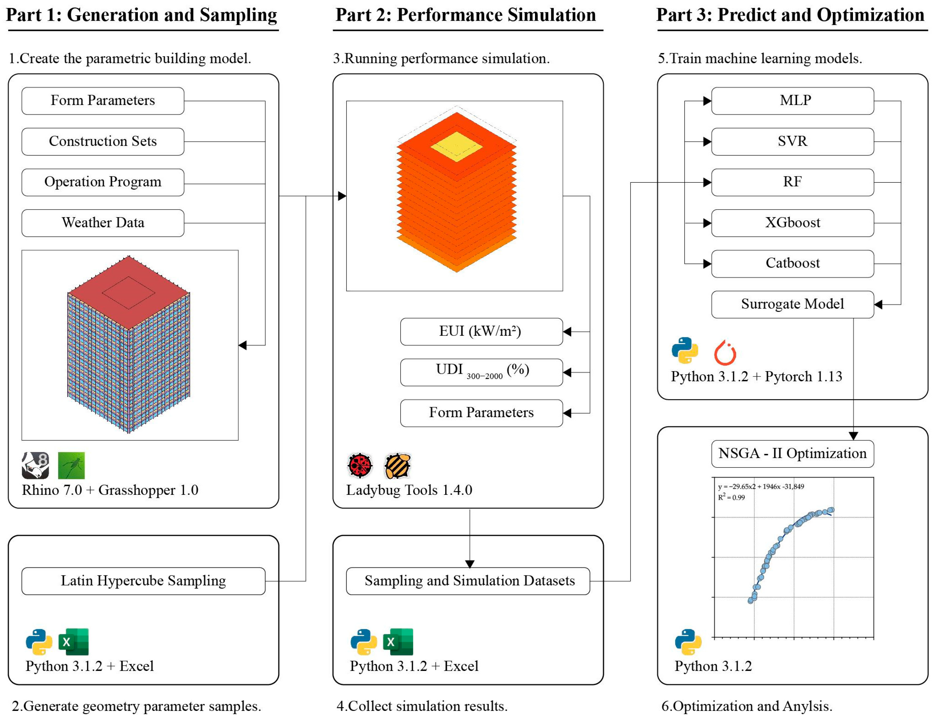
• Develop a form parametric model of typical high-rise office buildings in China’s HSWW zone, simulate their performance across diverse form parameter combinations, and train high-fidelity ML surrogate models for energy use intensity (EUI) and useful daylight illuminance (UDI).
• Integrate the surrogate models with GA to establish a computationally efficient multi-objective optimization workflow.
• Provide designers and policymakers with Pareto-optimal solutions and optimal architectural form parameter ranges for balancing energy efficiency and daylight levels in HSWW high-rise office buildings.

The paper is structured as follows: Section 2 outlines the methodology, including climate data selection for China’s HSWW zone; parametric model development using Rhino 7.0/Grasshopper 1.0; performance simulation via Ladybug Tools 1.4.0; machine learning (ML) algorithm selection criteria; and implementation of the GA-based optimization framework using Python 3.1.2. Section 3 discusses the accuracy of five ML models and presents Pareto-optimal solutions for EUI and UDI, along with corresponding optimal parameter distributions. Section 4 concludes the study, highlighting limitations and future research directions.

2. Methodology

As illustrated in Figure 1, the research framework comprises three interconnected phases.

Phase 1: Develop the parametric building model, which involves two core tasks: (1) defining parameters of architectural form (e.g., building orientation, building width, room depth, etc.), configuring the thermal parameter of the building envelope, selecting proper climate data files, and establishing occupancy schedules to create a parametric prototype of high-rise office buildings in China’s HSWW region; (2) generating datasets of parameter combinations via Latin hypercube sampling within the defined parameter ranges.

Phase 2: Run the performance simulation for each sampled building model using Ladybug Tools, generating a ‘parameter-performance’ dataset where each parameter combination is mapped to its corresponding EUI and UDI values.

Phase 3: Train multiple ML algorithms on the simulated datasets to develop surrogate models for multi-objective prediction. The best-performing models are integrated with the non-dominated sorting genetic algorithm (NSGA-II) to derive Pareto-optimal solutions. Based on the derived Pareto front, the optimal ranges and interactions of building design parameters are analyzed to identify performance trade-offs between EUI and UDI, thereby guiding design decision-making. The subsequent sections detail the tools and methodologies employed in each phase.

2.1. Development of Parametric Model

Given the morphological diversity of high-rise office buildings, a parametric prototype representing typical configurations in China’s HSWW zone was developed [70]. To enable efficient iterative design, Rhino/Grasshopper was selected as the modeling platform due to its visual programming environment, interoperability with simulation tools, and widespread adoption in performance-driven design [71]. The integration of Ladybug and Honeybee [72]—plugins leveraging EnergyPlus 9.6.0 and Radiance 5.4a [73]—allowed seamless connection between parametric modifications and multi-domain performance analysis.

Based on the survey of typical HSWW high-rise office buildings, the scope of parameters of architectural form was confirmed to guide the development of the parametric models. Parametric models were constructed for planar, vertical, and shading parameters, with each parameter adjustment automatically generating a new 3D model. To reduce model complexity and facilitate subsequent machine learning fitting, only 10 essential independent variables were selected to create the parametric model:

• In the planar aspect, the orientation parameter O, representing the rotation angle of the parametric model and simulating building orientation, changes in 15-degree steps and has its value range limited to half a full circle (180 degrees) due to the symmetrical plan. The plan width parameter W and aspect ratio parameter R define the planar size and shape, while the spatial depth parameter D determines the dimensions of office areas and core zones.
• In the vertical aspect, three parameters—floor height parameter FH, windowsill height parameter WSH, and ceiling height parameter CH—are sufficient to construct any common high-rise office facade. Notably, unlike most existing studies that rely on the commonly used window-to-wall ratio (WWR) parameter to control window/curtain wall size, this study utilizes WSH and CH to precisely define the size and vertical position of windows/curtain walls on the building facade. This allows for a more accurate assessment of how window size and placement influence the building’s performance.
• In the shading aspect, three parameters—horizontal sunshade size HSS, vertical sunshade size VSS, and vertical sunshade distance VSD—can model most common building shading configurations. In the parametric model, horizontal sunshades are fixed at the upper edge of windows/curtain walls, while vertical shading panels are evenly distributed along each facade at intervals defined by VSD. Both horizontal and vertical sunshades are oriented at a 90-degree angle to the facade.

By controlling the 10 parameters mentioned above, the parametric model can generate forms that match commonly found high-rise office building types in reality.

Figure 2 illustrates the parameters’ specific location on the building.

Table 1. Summary of form parameters.

Classification	Form Parameters	Range	Units	Steps	Properties	Baseline
Planar parameters	Orientation (O) 1	[0, 180]	degree	15	Independent	90
	Plan width (W)	[30, 50]	m	0.1	Independent	45
	Aspect ratio (R)	[1, 1.5]	-	0.05	Independent	1
	Spatial depth (D)	[8, 14]	m	-	Independent	12.5
	Plan length (L)	[30, 75]	m	-	Covariates 2	45
	Plan area (A)	[900, 3750]	m	-	Covariates 2	2025
Vertical parameters	Floor height (FH)	[3.9, 4.5]	m	0.1	Independent	4.2
	Ceiling height (CH)	[1, 1.5]	m	0.1	Independent	1.2
	Windowsill height (WSH)	[0.1, 1.2]	m	0.1	Independent	0.1
	Window height (WH)	[1.2, 3.4]	m	-	Covariates 2	2.9
	Window-wall ratio (WWR)	[30, 75]	%	-	Covariates 2	~69
	Building storey (BS) 3	15	-	-	Fixed	15
Shading parameters	Horizontal sunshade size (HSS)	[0.3, 1.5]	m	0.1	Independent	0.9
	Vertical sunshade size (VSS)	[0.3, 1.5]	m	0.1	Independent	0.9
	Vertical sunshade distance (VSD)	[3, 9]	m	0.1	Independent	3

¹ Orientation is represented numerically, with a 0–180 range due to the symmetric plan: 0° corresponds to west, 90° to south, and 180° to east. ² Covariate parameters are solely used for analytical purposes and excluded from machine learning input features. ³ The number of floors is fixed at 15—the average value for high-rise office buildings in China.

summarizes the value ranges and step sizes for all independent variables (covariates are derived from the independent parameters), while Figure 3 further visualizes several 3D models under different parametric configurations. Additionally, a set of parameters for the baseline model was established based on common high-rise office building typologies in the HSWW zone. The performance of the baseline model serves to quantify the improvement of the optimization through comparative analysis.

2.2. Specification of Material and Thermophysical Parameters

In addition to architectural form parameters, thermophysical properties for building envelope components (walls, windows, floors, and roofs) must also be determined for simulation accuracy. During early-stage simulations, detailed material layering was omitted in favor of simplified thermophysical values to balance accuracy and computational efficiency. Given the prevalence of green building standards in China’s new office construction, thermophysical and operational parameters were derived from the General Code for Energy Efficiency and Renewable Energy Utilization in Buildings (GB 55015-2021) [74] and the Energy Efficiency Design Standard for Public Buildings (GB 50189-2015) [75]. Where conflicts arose, the more recent GB 55015-2021 took precedence. For parameters not covered by Chinese codes, values from the ASHRAE 90.1-2019 standard [76] for Climate Zone 2A (corresponding to China’s HSWW zone) were adopted.

Table 2. Summary of thermophysical properties of the envelope.

Envelope		Thermal Conductivity [W/(m2·K)]	Solar Heat Gain Coefficient (SHGC)	Visible Transmittance
Curtain 1	Transmitting	1.5	-	-
	Opaque	2.4	0.2	0.6
Internal wall		2.1	-	-
Floor		1.1	-	-
Ground		1.5	-	-
Roof		0.4	-	-

¹ Curtain wall consists of two components: opaque cladding and transparent glazing.

presents the thermophysical properties assigned to each envelope component.

2.3. Setup of Building Operation Schedule

Since the energy consumption and light environment of an office building are closely related to its operation schedule, proper settings are necessary to achieve accurate simulation results. The building operation schedule can be meticulously configured using the Honeybee plugin. This plugin offers a “Program” port, which has eight sub-ports, including “People”, “Lighting”, “Electric Equipment”, “Gas Equipment”, “Hot Water”, “Infiltration”, “Ventilation”, and “Setpoint”. These sub-ports are used to define the device power, usage time, occupant density, and space occupancy rate.

For the sake of generality, the building operation schedule in this study is set according to the recommended values for office buildings in references [74,75]. The only difference is that the winter heating temperature specified in the standards is removed, and no heating equipment is used in winter. This adjustment aligns with the actual usage and design guidelines of most local office buildings in the HSWW zone. The detailed building operation schedule is presented in

Table 3. Summary of detailed building operation schedule.

Classification	Components	Values
People	Occupant heat power	120 W/people
	Occupant density	10 m2/people
	Occupant period	From 7 AM to 9 PM on weekdays
Lighting	Illuminance	300 lx
	Lighting power	8 W/m2
	Operating period	From 7 AM to 9 PM on weekdays
HVAC	Outdoor airflow rate	30 m3/(h × people)
	Cooling temperature setpoint	26 °C
	Heating temperature setpoint	Off 1
	Coefficient of Performance (COP)	4.0
	Operating period	From 7 AM to 9 PM on weekdays

¹ The heating function of the HVAC is deactivated by default, which better aligns with the typical operational patterns of office buildings in the HSWW zone.

.

2.4. Selection of Climate Dataset

China’s HSWW zone, one of the country’s five major climate regions, spans approximately 1.25 million km² across multiple provinces and cities. Figure 4 illustrates the geographical coverage of this climatic zone and the major cities within it. Characterized by monthly mean temperatures > 10 °C, July averages of 25–29 °C, and ≥25 °C daily temperatures for 100–200 days annually (with extreme highs reaching 40 °C) [77], the region’s vast geographic diversity necessitates careful selection of representative climate datasets for simulation accuracy. Figure 5 presents the monthly average temperatures and sunshine durations for the six major cities with the highest density of high-rise office buildings in China’s HSWW zone. All temperature and sunshine data are derived from the latest Typical Meteorological Year data (TMYx) provided by the U.S. National Oceanic and Atmospheric Administration (NOAA). The minimal differences between these cities, especially in the main cooling period, justify the selection of a single representative climate dataset to represent the zone. To ensure comparability with prior studies, this research adopted the .epw weather data of Guangzhou (China) to represent the climate of the HSWW zone.

Generally, open-source .epw data of Guangzhou were sourced from two repositories:

• CSWD (Chinese Standard Weather Data): A 2005 historical dataset provided by the China Meteorological Administration.
• TMYx (Typical Meteorological Year): A dynamically updated dataset from the U.S. NOAA, incorporating 2007–2021 monthly averages to reflect contemporary climate trends.

While CSWD has been widely used in Chinese studies, its static 2005 datasets may be less relevant to current conditions due to climate change. Figure 6 compares hourly dry bulb temperatures from the CSWD and TMYx datasets for Guangzhou, revealing significantly more high-temperature hours in TMYx. The average annual temperatures differ by 0.88 °C (22.23 °C for CSWD vs. 23.11 °C for TMYx), representing a 3.96% increase. Given the strong influence of ambient temperature on building energy use, TMYx data were selected to ensure up-to-date and realistic simulation outcomes.

2.5. Creation of Building Performance Simulation Datasets

Following parametric model development and simulation parameter configuration, energy and daylight simulations were executed using Honeybee 1.4.0 [78]—an open-source plugin for Grasshopper. This plugin’s computational accuracy has been validated in prior studies [79,80], ensuring reliable performance predictions.

To evaluate building performance, appropriate metrics were selected. For energy efficiency, energy use intensity (EUI, kWh/m²) was adopted, combining cooling energy (EUI_cooling) and lighting energy (EUI_lighting). Daylight performance was assessed using the Useful Daylight Index (UDI, %) proposed by Nabil and Mardaljevic [81], which quantifies the annual percentage of occupied hours with horizontal illuminance. Incorporating both glare and illuminance criteria, the UDI is widely recognized as a comprehensive metric for daylight quality. In this study, the UDI was calculated by placing sensors at 0.8 m above floor level (desk height) across a 1-m grid in office zones. The effective illuminance range of 300–2000 lux for typical office tasks was applied, and the final UDI value represented the average across all sensor points.

To enhance the representativeness, accuracy, and generalizability of the datasets for ML training, Latin hypercube sampling (LHS) was employed to generate parameter combinations. Latin hypercube sampling (LHS) efficiently captures design space variability without requiring excessive samples [82], meaning it has been widely adopted in building performance analysis [82,83,84]. This method ensures uniform parameter distribution while minimizing redundant sampling [17], making it particularly suitable for high-dimensional design spaces.

To achieve an optimal balance between computational cost and machine learning data requirements, a total of 50 parametric samples were generated. Simulations were executed on a 16-core CPU (AMD Ryzen^TM 9 7945HX, Advanced Micro Devices, Santa Clara, CA), taking approximately 10 min per sample simulation and totaling about 80 h for finishing the entire dataset.

2.6. Machine Learning Algorithm

As previously discussed, no single ML algorithm universally outperforms others in building performance analysis [85]. Predicting algorithm suitability for a specific dataset remains challenging prior to training. To address this, a comparative evaluation of multiple algorithms was conducted to identify the most accurate predictor. Given the impracticality of testing all available algorithms, selection criteria focused on algorithmic strengths and validated application scenarios. After comprehensive analysis, three algorithms were chosen for this study:

• Multi-Layer Perceptron (MLP): a prevalent and simple artificial neural network (ANN) architecture comprising input, hidden, and output layers was selected for this study due to its proven capacity to capture complex nonlinear relationships in building performance datasets. The input layer receives the parameters of architectural form, while the output layer generates predicted performance metrics. By incorporating nonlinear activation functions (e.g., ReLU, Sigmoid), MLPs can capture complex input-output relationships, making them well-suited for mapping static or low-dimensional time-series data like building design parameters to performance outcomes.
• Support Vector Regression (SVR): originating from support vector machine (SVM) theory [86], SVR is a regression model that maps low-dimensional data to a high-dimensional feature space using kernel functions (e.g., RBF). By constructing an optimal regression hyperplane, SVR effectively captures latent relationships between input and output variables, making it well-suited for predicting building performance metrics from design parameters. Unlike other continuous variable prediction methods, SVR exhibits robust generalization when applied to unseen data [87], maintaining superior predictive performance even with limited training data—a critical advantage for building optimization workflows constrained by computational resources.
• Random Forest (RF): an ensemble learning method that constructs multiple decision trees for classification and regression tasks, enhancing prediction accuracy and robustness through aggregating tree outputs [54]. This algorithm reduces model variance and mitigates overfitting risks via bootstrap sampling and random feature selection. Due to its insensitivity to noise and missing values, it maintains stable performance even with limited training data, which is a critical advantage over most other ML models. Additionally, tree-based models are favored for their interpretability, enabling transparent analysis of feature contributions to predictions [17].
• XGBoost: a powerful ensemble learning algorithm based on the Gradient Boosting Decision Tree (GBDT) [88]. It enhances prediction accuracy by combining multiple decision trees. Distinguishing itself from GBDT, XGBoost attains superior computational accuracy. It leverages the second-order Taylor expansion formula and incorporates a regularization term into the objective function, effectively mitigating overfitting risks. Currently, it has demonstrated advantages such as fast computation speed, high prediction accuracy, and strong robustness in regression problems and has become a very popular algorithm.
• CatBoost: an open-source GBDT framework developed by Yandex in 2017 [89] specifically designed for handling categorical features in classification, regression, and ranking tasks. Unlike traditional ML algorithms, CatBoost automates categorical feature processing through advanced techniques such as target encoding and combinatorial optimization, eliminating the need for manual pre-processing. This native capability makes CatBoost particularly suitable for unstructured datasets and high-cardinality categorical scenarios. Furthermore, it has demonstrated effectiveness in predicting energy consumption across diverse domains [90], where it often outperforms XGBoost in both prediction accuracy and computational efficiency.

To evaluate the predictive performance of different algorithms, three metrics were adopted: the coefficient of determination (R²), root mean squared error (RMSE), and coefficient of variation of RMSE (CVRMSE). R² (0 ≤ R² ≤ 1) quantifies the proportion of variance in the dependent variable explained by the model, with values closer to 1 indicating better fit. RMSE measures the average magnitude of prediction errors, calculated as the square root of the mean squared deviation between predicted and observed values. CVRMSE normalizes RMSE by the mean of observed values, yielding a dimensionless metric for fair cross-dataset comparisons. Recommended by ASHRAE [91], CVRMSE eliminates scale dependency and is particularly useful for benchmarking models across different building types or climates. The mathematical expressions for these metrics are provided in Equations (1)–(3).

$$R^2=1-{\displaystyle \frac{{\sum }_{\mathrm{i}=1}^{\mathrm{n}}{\left(y_i-{\check{y}}_i\right)}^2}{{\sum }_{\mathrm{i}=1}^{\mathrm{n}}{\left(y_i-{\overline{y}}_i\right)}^2}}$$

(1)

$$RMSE=\sqrt{{\sum }_{\mathrm{i}=1}^{\mathrm{n}}{\left({\check{y}}_i-{ y}_i\right)}^2/\mathrm{n}}$$

(2)

$$CVRMSE={\displaystyle \frac{\sqrt{{\sum }_{\mathrm{i}=1}^{\mathrm{n}}{\left({\check{y}}_i-{ y}_i\right)}^2/\mathrm{n}}}{{\sum }_{\mathrm{i}=1}^{\mathrm{n}}{y}_i/\mathrm{n}}}$$

(3)

where ${\check{y}}_i$, $y_i$, and ${\overline{y}}_i$ represent the predicted value of sample i, the actual value of sample i, and the mean value of all sample datasets, respectively; n denotes the number of samples.

2.7. Multi-Objective Optimization with Machine Learning

Upon establishing the surrogate model, multi-objective optimization was conducted using the Non-dominated Sorting Genetic Algorithm II (NSGA-II) [30] on Python. NSGA-II is a fast elitist algorithm renowned for its efficiency in low-dimensional optimization problems. Its elitism mechanism preserves the best solutions across generations by merging parent and offspring populations, ensuring convergence stability. NSGA-II may occasionally encounter duplicate solutions [30,92], but it remains the most widely adopted genetic algorithm in building optimization [93].

The optimization objective was to identify Pareto-optimal solutions minimizing EUI while maximizing useful daylight illuminance (UDI). Simulations were conducted in Python using the following NSGA-II parameters: population size: 200, generations: 50, crossover rate: 0.8, mutation rate: 0.9, and elitism ratio: 0.5. This parameter combination effectively maintained population diversity while avoiding prolonged convergence time.

3. Results and Discussion

3.1. Analysis of the Building Performance Datasets

Prior to implementing machine learning (ML), conducting a preliminary analysis of performance simulation results is crucial. This analysis aids researchers in refining ML model parameters (e.g., judging relevant variables) and identifying potential prediction issues (e.g., output distortion).

Figure 7 presents the statistical distributions of 500 simulation results for EUI and UDI. The data closely approximate normal distributions (R²_EUI = 0.94, R²_UDI = 0.98), validating the reliability of the simulation outcomes. The mean EUI of 34.02 kWh/m² is 1.67% higher than the baseline model, while the mean UDI of 70.91 is 3.71% lower, indicating the rationality of the baseline parameters. However, the baseline model’s EUI and UDI lag behind the simulation’s best results (EUI = 32.53, UDI = 81.70) by 2.78% and 11.1%, respectively, demonstrating substantial optimization potential for high-rise office buildings in the HSWW Zone.

Figure 8 presents Pearson correlation coefficients (r) between 10 architectural form parameters and building performance metrics. Pearson’s r quantifies the linear relationship strength between two variables, with values ranging from −1 to 1. Generally, |r| in the range of 0.3–0.5 indicates moderate correlation, while values > 0.5 mean a significantly strong correlation [94].

Heatmap analysis reveals that EUI exhibits strong negative correlations with HSS (horizontal sunshade size, r = −0.637), W (building width, r = −0.369), D (spatial depth, r = −0.395), WSH (windowsill height, r = −0.296), and VSS (vertical shading size, r = −0.286), indicating that larger shading devices, increased windowsill heights, and deeper spatial configurations reduce solar penetration and cooling energy consumption. For UDI, a strong negative correlation with D (space depth, r = −0.342) arises from limited daylight access in deep-plan spaces, while a moderate positive correlation with HSS (horizontal shading size, r = 0.496) suggests that expanded horizontal shading mitigates glare risks while maintaining adequate daylight levels.

3.2. Training and Evaluation of Machine Learning Models

The 500 simulated samples were randomly divided into 3 groups: 80% (400 samples) served as the training set, 10% (50 samples) were used for the validation set in an early stopping mechanism to prevent overfitting, and the remaining 10% (50 samples) formed the test set for validating prediction accuracy.

Table 4. The training results of the machine learning models.

Model Name	Results
	R2	RMSE	CVRMSE (%)
MLP	0.8728	0.2486	5.96%
SVR	0.4476	0.5182	37.89%
RF	0.8224	0.2938	15.1%
XGBoost	0.8672	0.2541	8.89%
CatBoost	0.9406	0.1930	1.57%

presents the training results of the five machine learning models. CatBoost outperformed all other algorithms, while MLP, XGBoost, and RF also demonstrated competitive performances. Notably, SVR performed poorly in this context. A key observation is that the top-performing models (CatBoost, XGBoost, and RF) are all ensemble learning algorithms, suggesting their potential superiority in predicting building performance using architectural form parameters. The CatBoost model, as the best performer, was selected for subsequent NSGA-II multi-objective optimization.

Figure 9 illustrates the training progression of the CatBoost model and its regression prediction performance. During training, both training and validation losses demonstrated sustained downward trends, indicating overall stability in the optimization process. The validation loss stabilized below 0.1 after approximately 18,000 iterations, at which point the model snapshot was selected as the final performance prediction surrogate model. Regression plots reveal that predicted outputs for the training, validation, and test sets align closely with target values along the diagonal, reflecting strong fitting relationships. This confirms the model’s capability to capture complex non-linear relationships between architectural form parameters and EUI/UDI.

Additionally, to evaluate whether the prediction model can be applied to performance prediction for high-rise office buildings in other cities within the HSWW zone, this study conducted performance predictions on 50 random parameter samples and simulated their actual EUI and UDI using the climate data of Shenzhen, which, similar to Guangzhou, also has a large number of high-rise office buildings in the region. The comparison results are shown in Figure 10. It can be observed that the actual EUI of high-rise office buildings in Shenzhen is generally slightly higher than that in Guangzhou, while the UDI is generally slightly lower. This result is likely due to two factors: (1) Shenzhen’s average temperature (23.89 °C) is approximately 3.50% higher than Guangzhou’s (23.08°C), which causes extra cooling consumption; and (2) the monthly hourly data of horizontal diffuse illuminance (HDI) above 10,000 lux in Shenzhen (119 h) are 4.2% higher than in Guangzhou (114 h), a factor that increases the likelihood of glare and decreases UDI.

When adjusting the ML model’s predictions by incorporating the 3.50% temperature difference and 4.2% monthly hourly HDI difference identified earlier, the average deviations between the adjusted predictions and Shenzhen’s actual data are approximately 1.33% and 1.80%, respectively. This indicates that after adjusting for climatic data differences, the prediction model demonstrates certain general predictive capabilities within the HSWW zone, and can be used in the early stages of architectural design where high precision is not required. However, for more detailed form optimization of buildings in specific cities, retraining the model with the target city’s simulation data is necessary.

3.3. Interpretability Analysis of Machine Learning Model Based on SHAP

Even when the CatBoost model exhibits a superior predictive performance, its predictions remain difficult to fully trust if the decision-making process remains opaque to human comprehension. Therefore, prior to engaging in performance optimization, conducting a rigorous interpretability analysis of the predictive model is essential. Interpretability refers to the systematic translation of complex model behaviors into causal frameworks understandable to humans, enabling researchers to discern the logical pathways underpinning model decisions.

As a variant of gradient-boosted decision trees (GBDT), CatBoost operates within a tree-based model [89]. Given the inherent explanatory advantages of SHAP (SHapley Additive exPlanation) [95] for tree-based models, this study employs SHAP to conduct interpretability analysis of the predictive model. Based on Shapley values from game theory, SHAP provides a theoretically rigorous framework to quantify the contribution of each feature to prediction outcomes [96]. SHAP not only ranks feature relevance but also elucidates the directional impact of individual features—how increases or decreases in a feature value influence the predicted result.

For the model developed in this study, SHAP quantifies the effect of each building’s form parameter on EUI and UDI by computing the average marginal contribution of each parameter across all possible feature combinations. This approach accounts for interactive effects between parameters, offering a comprehensive understanding of how form parameters collectively influence prediction results. The analytical process is conducted via the SHAP library in Python.

Figure 11 illustrates the importance ranking of each parameter for EUI and UDI based on SHAP values. The horizontal axis represents the average of the sum of absolute SHAP values across all samples, reflecting the influence of the form parameters on the two performance metrics.

In Figure 11a, HSS emerges as the most impactful parameter for EUI among all form factors, with a SHAP importance exceeding twice that of any other parameter. Parameters such as D, WSH, FH, VSD, and VSS show moderate effects on EUI, while O, R, W, and CH have negligible influences. For UDI, Figure 11b shows that HSS again has the strongest effect on UDI—parallel to its role in EUI—while D and FH exhibit notably significant impacts, with WSH, VSD, and CH contributing moderately. The remaining parameters, by contrast, have minimal effects on UDI.

Collectively, these results highlight that HSS is a critical factor for both EUI and UDI, underscoring the importance of horizontal shading design in the HSWW zone—consistent with prior Pearson analysis; parameters like D, FH, and WSH rank second, third, and fourth in importance, indicating substantial effects of spatial depth, floor height, and windowsill height on high-rise building performance. The lower importance of vertical sunshade parameters (VSS, VSD) indicates that horizontal sunshades are more critical than vertical counterparts; the higher ranking of WSH compared to CH implies greater optimization potential in adjusting windowsill height. Notably, D stands out as the only planar parameter with high importance, emphasizing that spatial depth impacts performance more significantly than building dimensions or shape.

Unlike importance ranking, SHAP beeswarm plots evaluate the positive or negative impacts of parameters on performance metrics: positive SHAP values indicate positive correlations, while negative values denote negative correlations, with larger absolute values reflecting stronger influences. Additionally, the color gradient of samples in these plots shows the relationship between parameter values and SHAP values, where redder colors indicate larger parameter values within their respective ranges, and bluer tones signify smaller values.

Analysis of the SHAP importance ranking plot also reveals that the SHAP importance of parameter CH for EUI is negligible, while its importance for UDI remains moderate. Although removing this parameter from ML model training might theoretically improve prediction performance, testing results indicate that excluding CH causes the model’s overall R² to drop from 0.94 to 0.70. This suggests that CH still plays a significant role in maintaining prediction accuracy.

Figure 12a presents the SHAP beeswarm plot for EUI, showing that W, R, D, WSH, HSS, and VSS correlate negatively with EUI. Among these parameters, HSS, WSH, and D exhibit particularly pronounced negative correlations, indicating that the larger sizes of horizontal sunshades, higher windowsills, and greater spatial depth reduce energy use in high-rise offices of the HSWW climate zone. Conversely, FH and VSD show positive correlations, indicating lower floor heights and smaller vertical shading distances are linked to lower energy consumption. O displays a non-linear relationship with energy use: intermediate O values (corresponding to south-facing orientations) are associated with reduced energy consumption, whereas decreases in O (west-facing) or increases in O (east-facing) correlate with higher energy use—likely due to balanced sunlight on south facades reducing extreme thermal loads compared to east/west orientations; CH has no significant directional trend, suggesting minimal direct impact on EUI.

Figure 12b presents the SHAP beeswarm plot for UDI, revealing that W, D, and VSD exhibit strong negative correlations with UDI—indicating that smaller plan widths, shallower spatial depths, and narrower vertical shading intervals enhance UDI. R demonstrates a moderate negative relationship with UDI, suggesting that building plans closer to a square configuration (lower R values) correlate with higher UDI; notably, a subset of samples with low R values display negative SHAP values, potentially attributable to model uncertainty or edge-case scenarios. Conversely, O, CH, and HSS show positive correlations with UDI: east-facing orientations, increased ceiling heights, and larger horizontal shading components consistently improve UDI performance. For HSS in particular, the beneficial effect is hypothesized to arise from its ability to filter direct solar radiation while preserving diffused light. Besides, FH, WSH, and VSS exhibit no clear directional trends, a result likely arising from strong interactive effects with other parameters.

Overall, the interpretability analysis of the prediction model using SHAP reveals the following results: Parameters HSS, D, FH, WSH, VSS, and VSD have substantial impacts on prediction outcomes. Larger horizontal sunshades and vertical sunshade sizes and minor southeast-facing orientations can reduce EUI while improving UDI. Conversely, greater building plan width and plan aspect ratio and spatial depth lower EUI but diminish UDI. Shorter floor heights (FH), higher windowsill heights (WSH), and narrower vertical sunshade intervals reduce EUI, though their effects on UDI require evaluation in conjunction with other parameters. Ceiling height has a minimal impact on EUI, yet larger CH values contribute to higher UDI.

These conclusions align well with practical design experience, underscoring the prediction model’s strong interpretability—whereby all parameters exert discernible effects on performance without irrelevant factors—thereby validating its credibility. Thus, this prediction model can be employed as a reliable surrogate for form parameter optimization via NSGA-II.

3.4. Performance and Analysis of Optimization

Leveraging the predictive capabilities of the surrogate model, the NSGA-II algorithm was implemented in Python to derive Pareto optimal solutions for EUI and UDI. Approximately 2 min of optimization yielded 65 Pareto-optimal solutions.

Figure 13 reveals that the solutions closely align with a quadratic curve (y = −29.65x² + 1946x − 31,849), reflecting a non-linear and competitive trade-off between EUI and UDI. In the initial segment, UDI increases at a higher rate with rising EUI, whereas in the latter part, UDI growth decelerates as EUI increases. Consequently, the convex point of the parabola is identified as the optimal design solution balancing both performance metrics.

However, these 65 Pareto-optimal solutions were predicted by the surrogate model. Although the surrogate model performed well on the testing data, deviations may still exist between its predictions and actual simulation results. To assess potential errors in these solutions, their corresponding form parameters were re-simulated using the original simulation tool. Figure 14 illustrates the discrepancies between re-simulated results and the initial Pareto solutions, presenting an average EUI difference rate of +0.34%, a UDI difference rate of −1.40%, and 8 solutions with difference rates between simulated and predicted values exceeding 5%. Figure 15 illustrates the distribution of normalized parameter values for these 8 samples within the complete set of optimal solutions, revealing that these outlier samples generally have larger values of W and D, as well as smaller FH and WSH. This suggests that the prediction model may produce certain deviations for a minority of parameter combinations at boundary conditions. While data processing and regularization techniques can mitigate these prediction discrepancies, their complete elimination remains unfeasible, highlighting the necessity of validating ML and GA optimization results through re-simulation.

After excluding the 8 solutions with difference rates > 5%, 57 Pareto-optimal solutions in close agreement with predictions were retained.

Table 5. Maximum, median, mean, and minimum values of the Pareto-optimal solutions for EUI/UDI, along with baseline model values.

Performance	Minimum	Maximum	Median	Mean	Baseline
EUI (kWh/m2)	31.95	33.21	32.36	32.45	33.46
UDI (%)	62.41	83.18	71.25	72.36	73.64

lists the maximum, median, mean, and minimum values for the two performances, along with the baseline model’s values.

Since solutions within the Pareto-optimal set are non-dominated and cannot be directly ranked [97], designers should select appropriate designs based on their preferences. For energy minimization, the solution with the lowest EUI (31.95 kWh/m², 4.51% lower than the baseline model) can be chosen, but it reduces UDI by 9.70% compared to the baseline model. Conversely, maximizing the UDI solution (83.18%, 13.0% higher than baseline) increases EUI by 1.34%. For balanced performance, the convex point of the Pareto-optimal is recommended. Five solutions at the convex point achieve both metrics better than the baseline: a mean EUI of 32.35 kWh/m² (3.31% lower than the baseline) and a mean UDI of 77.41% (5.12% higher than the baseline). These results demonstrate the effectiveness of the optimization framework in balancing energy efficiency and daylight performance.

However, in practical design scenarios, designers and decision-makers rarely adopt optimal parameters directly due to various subjective and objective constraints. Instead, the Pareto-optimal set also provides numerical references through the maximum, minimum, and median values of each form parameter across the Pareto-optimal solutions. Figure 16, Figure 17 and Figure 18 present the parameter distributions of Pareto-optimal solutions using box plots, categorized into three aspects: planar parameters, vertical parameters, and shading parameters.

Figure 16 illustrates the distribution of planar parameters for Pareto-optimal solutions. Orientations within the Pareto set cluster are at 105° (15° east of south), with secondary frequency peaks at 90° (south) and 120° (30° east of south). This clustering indicates that southeast/south-facing orientations are optimal for high-rise office buildings in this region, as they align with prevailing monsoon patterns—enhancing natural ventilation and reducing west-facing solar heat gain, which minimizes cooling loads. The median plan width and length values are 40.2 m and 58.3 m, and a dominant 1.45 aspect ratio (length/width) implies that increasing the south-facing facade area improves performance. Spatial depth and plan area cluster at 9 m/1500 m² and 12 m/2500 m², indicating an adaptive strategy balancing daylight access (shallow and small plans) and heat reduction (deep and large plans).

Figure 17 shows the distribution of vertical parameters for Pareto-optimal solutions. Floor heights ranging from 4.1 to 4.3 m reflect a balance between daylight volume and spatial comfort. The maximum allowable values for windowsill (1.2 m) and ceiling heights (1.4 m) indicate that reduced window area contributes to enhanced overall building performance, which is supported by window height distributions (1.4–1.9 m) and WWR (~0.3).

Figure 18 presents the distribution of vertical parameters for Pareto-optimal solutions. The uniform adoption of 1.5 m horizontal sunshade size and 3 m vertical sunshade intervals, both representing minimum design thresholds, highlights their critical role in performance optimization. While vertical sunshade sizes contribute less significantly than horizontal shading, larger vertical sunshades are still preferentially selected in optimal solutions. This parameter distribution evinces their supplementary role in mitigating solar heat gain and reducing excessive direct solar radiation that causes indoor overheating and discomfort glare, thereby minimizing cooling loads while addressing glare-related visual disturbances.

Collectively, these findings identify enlarger shading systems, southeast/south orientations, substantially large or small spatial depths, high aspect ratios, and reduced window areas as key determinants in balancing EUI and UDI for high-rise office building performance in China’s HSWW zone. Additionally, the observed parameter distribution patterns and median values of Pareto-optimal solutions provide meaningful design guidelines for such buildings in this climate zone, offering valuable references for future practices that balance energy efficiency and visual comfort criteria.

4. Conclusions

This study proposes a performance-oriented optimization method for building morphology, integrating machine learning (ML) algorithms with genetic algorithms (GAs), and establishes a complete workflow. Guided by this framework, this paper uses Guangzhou as a case study in China’s HSWW climate zone to optimize the form parameters of local high-rise office buildings. The primary findings are as follows:

• Through comparative analysis of multiple ML algorithms, ensemble ML algorithms are found to effectively capture the complex nonlinear relationships between building form parameters and performance metrics. Among them, the CatBoost algorithm demonstrates the best predictive performance for this study’s target (R² = 0.94, CVRMSE = 1.59%).
• SHAP analysis shows that horizontal sunshade size (HSS), spatial depth (D), floor height (FH), windowsill height (WSH), vertical sunshade size (VSS), and vertical shading distance (VSD) strongly influence the predictions of the machine learning model. Additionally, by increasing horizontal sunshade sizes, decreasing vertical shading distance, and adjusting building orientation to a slight southeast direction, these form parameters become the most effective for performance optimization, achieving reduced EUI while improving UDI. In general, SHAP analysis indicates that shading parameters have the greatest effect on performance results, followed by vertical parameters, with planar parameters exerting the smallest influence.
• The Pareto-optimal morphological parameters generated by the surrogate model show good agreement with their corresponding actual simulation results, with 87.7% (57 out of 65) of the results having an error rate below 5% and an average error rate of 0.34% for EUI and −1.4% for UDI. This demonstrates the effectiveness of the integrated optimization approach using machine learning and genetic algorithms.
• Compared to the baseline model, a Pareto-optimal solution achieves a 3.31% reduction in EUI and a 5.12% increase in UDI.
• Based on the Pareto-optimal solutions, the following design strategies for form parameters are proposed to fully enhance the energy-saving potential of high-rise office buildings in China’s HSWW zone: (1) adopting a building orientation ranging from due south to 30 degrees east of south; (2) using a rectangular floor plan measuring approximately 40 m in width and 58 m in length (an aspect ratio of 1.45, total area of about 2300 m², and office area depth of 12 m); (3) implementing a facade design with a floor height of 4.0–4.2 m, larger possible windowsill and ceiling height, and a window-to-wall ratio of 0.37–0.45; and (4) employing horizontal and vertical sunshades longer than 1.3 m as well as high-density vertical sunshades.

However, this research has several limitations. First, the parametric model only uses 10 constrained form parameters, which are insufficient for designs requiring greater precision, although they are suitable for most early-stage design processes. Second, only two performance objectives were selected, lacking consideration of other metrics (e.g., thermal comfort, carbon emissions). Third, the algorithm comparison was limited to five well-established classical algorithms, without exploring advanced algorithms or deep neural network approaches. Additionally, this study only chose Guangzhou as a representative of this climate zone. Although cities within the same climate zone share similar climatic conditions, there are still subtle differences between them, which may lead to certain deviations in the optimal results.

Future research should focus on the following directions: (1) applying the proposed method to building designs with more parameters, such as the rotation angles of shading devices and other geometric details; (2) incorporating additional performance objectives; (3) investigating advanced machine learning (ML) algorithms to improve prediction accuracy; (4) extending this research method to more cities within this climate zone to obtain more precise form optimization results and attempting to develop a universal prediction model applicable to all major cities in this climate zone; (5) applying this method to the form optimization of high-rise office buildings in other climatic zones of China; and (6) extending the simulation duration to account for long-term climate change impacts.

References

1. WMO Confirms That 2023 Smashes Global Temperature Record. Available online: https://wmo.int/news/media-centre/wmo-confirms-2023-smashes-global-temperature-record (accessed on 15 March 2025).
2. The 2019 Blue Book on Climate Change in China. Available online: https://www.cma.gov.cn/zfxxgk/gknr/qxbg/201905/t20190524_1709279.html (accessed on 15 March 2025).
3. United Nations; Intergovernmental Panel on Climate Change (IPCC). Climate Change 2013: The Physical Science Basis; Plattner, M., Ed.; Cambridge University Press: Cambridge, UK, 2013. [Google Scholar]
4. Geng, Y.; Sarkis, J. China-US trade spat could hit the environment. Nature 2018, 557, 309. [Google Scholar] [CrossRef] [PubMed]
5. China Association of Building Energy Efficiency; Chongqing University. Research Report on Energy Consumption and Carbon Emission of Buildings in China (2023). Construct Archit. 2024, 2024, 46–59. [Google Scholar]
6. Reshaping Energy: A Study on the Roadmap of China’s Energy Consumption and Production Revolution Towards 2050. 2016. Available online: https://china.lbl.gov (accessed on 15 March 2025).
7. China Association of Building Energy Efficiency. 2022 Research Report of China Building Energy Consumption and Carbon Emissions; China Association of Building Energy Efficiency: Chongqing, China, 2023; Volume 27, p. 12. [Google Scholar]
8. Ma, M.; Cai, W.; Wu, Y. China Act on the Energy Efficiency of Civil Buildings (2008): A decade review. Sci. Total Environ. 2019, 651, 42–60. [Google Scholar] [CrossRef] [PubMed]
9. Song, L.; Zhang, C.; Li, H.J. 2015 National Green Building Evaluation Label Statistical Report. Constr. Sci. Technol. 2016, 10, 12–15. [Google Scholar] [CrossRef]
10. Ruparathna, R.; Hewage, K.; Sadiq, R. Improving the energy efficiency of the existing building stock: A critical review of commercial and institutional buildings. Renew. Sustain. Energy Rev. 2016, 53, 1032–1045. [Google Scholar] [CrossRef]
11. The Ministry of Housing and Urban Rural Development of China. Several Opinions of the Ministry of Housing and Urban Rural Development on Promoting the Development and Reform of the Construction Industry. Intell. Build. City Inf. 2014, 7, 24–28. [Google Scholar]
12. American Society of Heating, Refrigeration and Air-Conditioning Engineers. ASHRAE Handbook: Fundamentals; ASHRAE: Atlanta, GA, USA, 2009. [Google Scholar]
13. EnergyPlus. Available online: https://energyplus.net/ (accessed on 15 March 2025).
14. TRNSYS: Transient System Simulation Tool. Available online: http://www.trnsys.com/ (accessed on 15 March 2025).
15. Lin, B.; Chen, H.; Liu, Y.; He, Q.; Li, Z. A Preference-Based Multi-Objective Building Performance Optimization Method for Early Design Stage. Build. Simul. 2021, 14, 477–494. [Google Scholar] [CrossRef]
16. Li, Y.; O’Neill, Z.; Zhang, L.; Chen, J.; Im, P.; DeGraw, J. Grey-box modeling and application for building energy simulations—A critical review. Renew. Sustain. Energy Rev. 2021, 146, 111–174. [Google Scholar] [CrossRef]
17. Manmatharasan, P.; Bitsuamlak, G.; Grolinger, K. AI-driven design optimization for sustainable buildings: A systematic review. Energy Build. 2025, 332, 115440. [Google Scholar] [CrossRef]
18. Clarke, J.A.; Clarke, J.A. Energy Simulation in Building Design; Routledge: London, UK, 2001. [Google Scholar]
19. Javanroodi, K.; Nik, V.M.; Mahdavinejad, M. A novel design—Based optimization framework for enhancing the energy efficiency of high-rise office buildings in urban areas. Sustain. Cities Soc. 2019, 49, 101577. [Google Scholar] [CrossRef]
20. Božiček, D.; Kunič, R.; Krainer, A.; Stritih, U.; Dovjak, M. Mutual Influence of External Wall Thermal Transmittance, Thermal Inertia, and Room Orientation on Office Thermal Comfort and Energy Demand. Energies 2023, 16, 3524. [Google Scholar] [CrossRef]
21. Soflaei, F.; Shokouhian, M.; Tabadkani, A.; Moslehi, H.; Berardi, U. A simulation-based model for courtyard housing design based on adaptive thermal comfort. J. Build. Eng. 2020, 31, 101335. [Google Scholar] [CrossRef]
22. Du, Y.; Mak, C.M.; Li, Y. A multi-stage optimization of pedestrian level wind environment and thermal comfort with lift-up design in ideal urban canyons. Sustain. Cities Soc. 2019, 46, 101424. [Google Scholar] [CrossRef]
23. Moazzeni, M.H.; Ghiabaklou, Z. Investigating the Influence of Light Shelf Geometry Parameters on Daylight Performance and Visual Comfort, a Case Study of Educational Space in Tehran, Iran. Buildings 2016, 6, 26. [Google Scholar] [CrossRef]
24. Alhagla, K.; Mansour, A.; Elbassuoni, R. Optimizing windows for enhancing daylighting performance and energy saving. Alex. Eng. J. 2019, 58, 283–290. [Google Scholar] [CrossRef]
25. Susa-Páez, A.; Piderit-Moreno, M.B. Geometric Optimization of Atriums with Natural Lighting Potential for Detached High-Rise Buildings. Sustainability 2020, 12, 6651. [Google Scholar] [CrossRef]
26. Gan, V.J.L.; Wang, B.; Chan, C.M.; Weerasuriya, A.U.; Cheng, J.C.P. Physics-based, data-driven approach for predicting natural ventilation of residential high-rise buildings. Build. Simul. 2022, 15, 129–148. [Google Scholar] [CrossRef]
27. Østergård, T.; Jensen, R.L.; Maagaard, S.E. Building simulations supporting decision making in early design—A review. Renew. Sustain. Energy Rev. 2016, 61, 187–201. [Google Scholar] [CrossRef]
28. Wortmann, T.; Cichocka, J.; Waibel, C. Simulation-based optimization in architecture and building engineering—Results from an international user survey in practice and research. Energy Build. 2022, 259, 111863. [Google Scholar] [CrossRef]
29. Radford, A.D.; Gero, J.S. On optimization in computer aided architectural design. Build. Environ. 1980, 15, 73–80. [Google Scholar] [CrossRef]
30. Deb, K. Multi-Objective Optimization Using Evolutionary Algorithm; John Wiley & Sons: Hoboken, NJ, USA, 2001; p. 497. [Google Scholar]
31. Longo, S.; Montana, F.; Riva Sanseverino, E. A review on optimization and cost-optimal methodologies in low-energy buildings design and environmental considerations. Sustain. Cities Soc. 2019, 45, 87–104. [Google Scholar] [CrossRef]
32. Attia, S. Computational Optimisation for Zero Energy Building Design, Interviews with Twenty Eight International Experts. In Proceedings of the Building Simulation 2013—13th International IBPSA Conference, Chambery, France, 25–28 August 2012; Architecture et Climat: Paris, France, 2012. [Google Scholar]
33. Wetter, M.; Wright, J.A. A comparison of deterministic and probabilistic optimization algorithms for nonsmooth simulation—Based optimization. Build. Environ. 2004, 39, 989–999. [Google Scholar] [CrossRef]
34. Hamdy, M.; Nguyen, A.-T.; Hensen, J.L.M. A performance comparison of multi-objective optimization algorithms for solving nearly-zero-energy-building design problems. Energy Build. 2016, 121, 57–71. [Google Scholar] [CrossRef]
35. modeFRONTIER. Available online: http://www.esteco.com/modefrontier (accessed on 15 March 2025).
36. Octopus. Available online: https://www.grasshopper3d.com/group/octopus?overrideMobileRedirect=1 (accessed on 15 March 2025).
37. Alelwani, R.; Ahmad, M.W.; Rezgui, Y.; Alshammari, K. Optimising Energy Efficiency and Daylighting Performance for Designing Vernacular Architecture—A Case Study of Rawshan. Sustainability 2025, 17, 315. [Google Scholar] [CrossRef]
38. Wang, M.; Xu, Y.; Shen, R.; Wu, Y. Performance—Oriented Parametric Optimization Design for Energy Efficiency of Rural Residential Buildings: A Case Study from China’s Hot Summer and Cold Winter Zone. Sustainability 2024, 16, 8330. [Google Scholar] [CrossRef]
39. Chaturvedi, S.; Rajasekar, E.; Natarajan, S. Multi-objective Building Design Optimization under Operational Uncertainties Using the NSGA II Algorithm. Buildings 2020, 10, 88. [Google Scholar] [CrossRef]
40. Zhao, J.; Du, Y. Multi-objective optimization design for windows and shading configuration considering energy consumption and thermal comfort: A case study for office building in different climatic regions of China. Sol. Energy 2020, 206, 997–1017. [Google Scholar] [CrossRef]
41. Amasyali, K.; El-Gohary, N.M. A review of data-driven building energy consumption prediction studies. Renew. Sustain. Energy Rev. 2018, 81, 1192–1205. [Google Scholar] [CrossRef]
42. Qiao, Q.; Yunusa-Kaltungo, A.; Edwards, R.E. Towards developing a systematic knowledge trend for building energy consumption prediction. J. Build. Eng. 2021, 35, 101967. [Google Scholar] [CrossRef]
43. Zhang, L.; Wen, J.; Li, Y.; Chen, J.; Ye, Y.; Fu, Y.; Livingood, W. A review of machine learning in building load prediction. Appl. Energy 2021, 285, 116452. [Google Scholar] [CrossRef]
44. Kalogirou, S.A. Applications of artificial neural-networks for energy systems. Appl. Energy 2000, 67, 17–35. [Google Scholar] [CrossRef]
45. Wong, S.L.; Wan, K.K.W.; Lam, T.N.T. Artificial neural networks for energy analysis of office buildings with daylighting. Appl. Energy 2010, 87, 551–557. [Google Scholar] [CrossRef]
46. Moon, J.W.; Kim, J.-J. ANN-based thermal control models for residential buildings. Build. Environ. 2010, 45, 1612–1625. [Google Scholar] [CrossRef]
47. Geyer, P.; Singaravel, S. Component-based machine learning for performance prediction in building design. Appl. Energy 2018, 228, 1439–1453. [Google Scholar] [CrossRef]
48. Shao, M.; Wang, X.; Bu, Z.; Chen, X.; Wang, Y. Prediction of energy consumption in hotel buildings via support vector machines. Sustain. Cities Soc. 2020, 57, 102128. [Google Scholar] [CrossRef]
49. Liu, Y.; Chen, H.; Zhang, L.; Wu, X.; Wang, X. -J. Energy consumption prediction and diagnosis of public buildings based on support vector machine learning: A case study in China. J. Clean. Prod. 2020, 272, 122542. [Google Scholar] [CrossRef]
50. Cai, W.; Wen, X.; Li, C.; Shao, J.; Xu, J. Predicting the energy consumption in buildings using the optimized support vector regression model. Energy 2023, 273, 127188. [Google Scholar] [CrossRef]
51. Wu, C.; Pan, H.; Luo, Z.; Liu, C.; Huang, H. Multi-objective optimization of residential building energy consumption, daylighting, and thermal comfort based on BO-XGBoost-NSGA-II. Build. Environ. 2024, 254, 111386. [Google Scholar] [CrossRef]
52. Yan, K.; Li, W.; Ji, Z.; Qi, M.; Du, Y. A Hybrid LSTM Neural Network for Energy Consumption Forecasting of Individual Households. IEEE Access 2019, 7, 157633–157642. [Google Scholar] [CrossRef]
53. Yu, Z.; Haghighat, F.; Fung, B.C.M.; Yoshino, H. A decision tree method for building energy demand modeling. Energy Build. 2010, 42, 1637–1646. [Google Scholar] [CrossRef]
54. Breiman, L. Random forests. Mach. Learn. 2001, 45, 5–32. [Google Scholar] [CrossRef]
55. Wang, Z.; Wang, Y.; Zeng, R.; Srinivasan, R.S.; Ahrentzen, S. Random Forest based hourly building energy prediction. Energy Build. 2018, 171, 11–25. [Google Scholar] [CrossRef]
56. Pham, A.-D.; Ngo, N.-T.; Truong, T.T.H.; Huynh, N.-T.; Truong, N.-S. Predicting energy consumption in multiple buildings using machine learning for improving energy efficiency and sustainability. J. Clean. Prod. 2020, 260, 121082. [Google Scholar] [CrossRef]
57. Chi, B.; Li, Y.; Zhou, D. A Hybrid Method of Cooling and Heating Consumption Prediction for Six Types of Buildings Based on Machine Learning. Sustainability 2024, 16, 11200. [Google Scholar] [CrossRef]
58. Safarzadegan Gilan, S.; Goyal, N.; Dilkina, B. Active learning in multi-objective evolutionary algorithms for sustainable building design. In Proceedings of the Genetic and Evolutionary Computation Conference 2016, Denver, CO, USA, 20–24 July 2016. [Google Scholar]
59. Chen, X.; Yang, H. A multi-stage optimization of passively designed high-rise residential buildings in multiple building operation scenarios. Appl. Energy 2017, 206, 541–557. [Google Scholar] [CrossRef]
60. Gou, S.; Nik, V.M.; Scartezzini, J.L.; Zhao, Q.; Li, Z. Passive design optimization of newly-built residential buildings in Shanghai for improving indoor thermal comfort while reducing building energy demand. Energy Build. 2018, 169, 484–506. [Google Scholar] [CrossRef]
61. Ilbeigi, M.; Ghomeishi, M.; Dehghanbanadaki, A. Prediction and optimization of energy consumption in an office building using artificial neural network and a genetic algorithm. Sustain. Cities Soc. 2020, 61, 102325. [Google Scholar] [CrossRef]
62. Chen, R.; Tsay, Y.-S.; Ni, S. An integrated framework for multi-objective optimization of building performance: Carbon emissions, thermal comfort, and global cost. J. Clean. Prod. 2022, 359, 131978. [Google Scholar] [CrossRef]
63. Ding, Z.; Li, J.; Wang, Z.; Xiong, Z. Multi-Objective Optimization of Building Envelope Retrofits Considering Future Climate Scenarios: An Integrated Approach Using Machine Learning and Climate Models. Sustainability 2024, 16, 8217. [Google Scholar] [CrossRef]
64. Si, B.; Ni, Z.; Xu, J.; Li, Y.; Liu, F. Interactive effects of hyperparameter optimization techniques and data characteristics on the performance of machine learning algorithms for building energy metamodeling. Case Stud. Therm. Eng. 2024, 55, 104124. [Google Scholar] [CrossRef]
65. Al-Masrani, S.M.; Al-Obaidi, K.M. Dynamic shading systems: A review of design parameters, platforms and evaluation strategies. Autom. Constr. 2019, 102, 195–216. [Google Scholar] [CrossRef]
66. Zhou, F.; Wang, Z.; Su, X.; Yang, Y.; Duanmu, L.; Zhou, X.; Lian, Z.; Zhai, Y.; Cao, B.; Zhang, Y.; et al. Study on the Thermal Adaptation Model During the Transition Season in Hot Summer and Cold Winter Regions. Heat. Vent. Air Cond. 2022, 52, 132–136. [Google Scholar] [CrossRef]
67. Kheiri, F. A review on optimization methods applied in energy-efficient building geometry and envelope design. Renew. Sustain. Energy Rev. 2018, 92, 897–920. [Google Scholar] [CrossRef]
68. Li, S.; Liu, L.; Peng, C. A Review of Performance-Oriented Architectural Design and Optimization in the Context of Sustainability: Dividends and Challenges. Sustainability 2020, 12, 1427. [Google Scholar] [CrossRef]
69. Xuanyuan, P.; Zhang, Y.; Yao, J.; Zheng, R. Sensitivity Analysis and Optimization of Energy-Saving Measures for Office Building in Hot Summer and Cold Winter Regions. Energies 2024, 17, 1675. [Google Scholar] [CrossRef]
70. Ma, Y.; Deng, W.; Xie, J.; Heath, T.; Xiang, Y.; Hong, Y. Generating prototypical residential building geometry models using a new hybrid approach. Build. Simul. 2022, 15, 17–28. [Google Scholar] [CrossRef]
71. Touloupaki, E.; Theodosiou, T. Performance Simulation Integrated in Parametric 3D Modeling as a Method for Early Stage Design Optimization—A Review. Energies 2017, 10, 637. [Google Scholar] [CrossRef]
72. Honeybee for Grasshopper. Available online: https://github.com/mostaphaRoudsari/Honeybee/ (accessed on 15 March 2025).
73. Ward, G.J. The Radiance lighting simulation and rendering system. In Proceedings of the 21st Annual Conference on Computer Graphics and Interactive Techniques, SIGGRAPH, Orlando, FL, USA, 24–29 July 1994. [Google Scholar]
74. GB 55015-2021; General Specification for Building Energy Efficiency and Renewable Energy Utilization. China Architecture & Building Press: Beijing, China, 2022.
75. GB 50189-2015; General Administration of Quality Supervision, Inspection and Quarantine of the People’s Republic of China. Design Standard for Energy Efficiency of Public Buildings. China Architecture & Building Press: Beijing, China, 2015.
76. ASHRAE Standard 90.1-2019; Energy Standard for Buildings Except Low-Rise Residential Buildings. ASHRAE: Atlanta, GA, USA, 2019.
77. GB 50352-2019; Unified Standard for Civil Building Design. China Architecture & Building Press: Beijing, China, 2014.
78. Honeybee. Available online: https://www.ladybug.tools/honeybee.html (accessed on 15 March 2025).
79. Roudsari, M.S.; Pak, M.; Smith, A. Ladybug: A parametric environmental plugin for grasshopper to help designers create an environmentally-conscious design. In Proceedings of the 13th International IBPSA Conference, Lyon, France, 25–28 August 2013; Volume 8. [Google Scholar]
80. Negendahl, K.; Nielsen, T.R. Building energy optimization in the early design stages: A simplified method. Energy Build. 2015, 105, 88–99. [Google Scholar] [CrossRef]
81. Nabil, A.; Mardaljevic, J. Useful daylight illuminance: A new paradigm for assessing daylight in buildings. Light Res. Technol. 2005, 37, 41–57. [Google Scholar] [CrossRef]
82. Tian, W. A review of sensitivity analysis methods in building energy analysis. Renew. Sustain. Energy Rev. 2013, 20, 411–419. [Google Scholar] [CrossRef]
83. Mahmoud, A.H.A.; Elghazi, Y. Parametric-based designs for kinetic facades to optimize daylight performance: Comparing rotation and translation kinetic motion for hexagonal facade patterns. Solar Energy 2016, 126, 111–127. [Google Scholar] [CrossRef]
84. Helton, J.C.; Johnson, J.D.; Sallaberry, C.J.; Storlie, C.B. Survey of sampling-based methods for uncertainty and sensitivity analysis. Reliab. Eng. Syst. Saf. 2006, 91, 1175–1209. [Google Scholar] [CrossRef]
85. Ascione, F.; Bianco, N.; De Stasio, C.; Mauro, G.M.; Vanoli, G.P. Artificial neural networks to predict energy performance and retrofit scenarios for any member of a building category: A novel approach. Energy 2017, 118, 999–1017. [Google Scholar] [CrossRef]
86. Drucker, H.; Burges, C.J.; Kaufman, L.; Smola, A.; Vapnik, V. Support vector regression machines. Adv. Neural Inf. Process. Syst. 1997, 9, 155–161. [Google Scholar]
87. Jain, R.K.; Smith, K.M.; Culligan, P.J.; Taylor, J.E. Forecasting energy consumption of multi-family residential buildings using support vector regression: Investigating the impact of temporal and spatial monitoring granularity on performance accuracy. Appl. Energy 2014, 123, 168–178. [Google Scholar] [CrossRef]
88. Chen, T.; Guestrin, C. XGBoost: A scalable tree boosting system. In Proceedings of the KDD’16: Proceedings of the 22nd ACM SIGKDD International Conference on Knowledge Discovery and Data Mining, Hong Kong, China, 13–17 August 2016; Volume 9, p. 3. [Google Scholar] [CrossRef]
89. Yandex. CatBoost: Gradient Boosting with Categorical Features. Available online: https://catboost.ai (accessed on 16 March 2025).
90. Bian, J.; Wang, J.; Yece, Q. A novel study on power consumption of an HVAC system using CatBoost and AdaBoost algorithms combined with the metaheuristic algorithms. Energy 2024, 302, 131841. [Google Scholar] [CrossRef]
91. American Society of Heating, Refrigerating and Air-Conditioning Engineers. Measurement of Energy and Demand Savings (ASHRAE Guideline 14-2014); ASHRAE: Atlanta, GA, USA, 2014. [Google Scholar]
92. Deb, K.; Agrawal, S.; Pratap, A.; Meyarivan, T. A fast elitist non-dominated sorting genetic algorithm for multi-objective optimization: NSGA-II. In Proceedings of the International Conference on Parallel Problem Solving from Nature, Paris, France, 18–20 September 2000; pp. 849–858. [Google Scholar] [CrossRef]
93. Delgarm, N.; Sajadi, B.; Delgarm, S.; Kowsary, F. A novel approach for the simulation-based optimization of the buildings energy consumption using NSGA-II: Case study in Iran. Energy Build. 2016, 127, 552–560. [Google Scholar] [CrossRef]
94. Cohen, J. Statistical Power Analysis for the Behavioral Sciences, 2nd ed.; Lawrence Erlbaum Associates: Mahwah, NJ, USA, 1988. [Google Scholar]
95. Lundberg, S.; Lee, S. A unified approach to interpreting model predictions. In Proceedings of the 31st International Conference on Neural Information Processing Systems (NIPS’17), Long Beach, CA, USA, 4–9 December 2017; Volume 4, p. 12. [Google Scholar]
96. Salih, A.M.; Raisi-Estabragh, Z.; Galazzo, I.B.; Radeva, P.; Petersen, S.E.; Lekadir, K.; and Menegaz, G. A Perspective on Explainable Artificial Intelligence Methods: SHAP and LIME. Adv. Intell. Syst. 2024, 7, 2400304. [Google Scholar] [CrossRef]
97. Suga, K.; Kato, S.; Hiyama, K. Structural analysis of Pareto-optimal solution sets for multi-objective optimization: An application to outer window design problems using Multiple Objective Genetic Algorithms. Build. Environ. 2010, 45, 1144–1152. [Google Scholar] [CrossRef]
Figure 1. Research framework.
Sustainability 17 04090 g001
Figure 2. The references for each parameter: (a) reference of the planar parameters. For planar parameters, the plan length can be calculated as W × R, and the core (circulation and other non-support office spaces) size automatically adapts to W, R, and D. (b) Reference of the vertical and shading parameters, the height of the window can be given by FH − (CH + WSH).
Sustainability 17 04090 g002
Figure 3. 3D models generated via different parametric configurations, showcasing the capability of the parametric model with 10 form parameters.
Sustainability 17 04090 g003
Figure 4. The geographical coverage of China’s HSWW climate zone and the major cities within it. The red star represents the location of Beijing, the capital of China.
Sustainability 17 04090 g004
Figure 5. The climate differences between six major cities in the HSWW zone: (a) monthly average temperature; (b) monthly average sunshine duration.
Sustainability 17 04090 g005
Figure 6. Comparison of hourly dry bulb temperatures of Guangzhou from CSWD and TMYx datasets: (a) hourly temperatures of Guangzhou from CSWD with less red color (representing high temperature); (b) hourly temperatures of Guangzhou for TMYx with more red color.
Sustainability 17 04090 g006
Figure 7. Frequency distribution plot of EUI and UDI values: (a) frequency distribution plot of EUI; (b) frequency distribution plot of UDI.
Sustainability 17 04090 g007
Figure 8. Heatmap of Pearson correlation coefficients (r) between building form parameters and EUI/UDI.
Sustainability 17 04090 g008
Figure 9. Training progression of the CatBoost model and its regression prediction performance: (a) MSE changes during iterations; (b) regression of training data; (c) regression of validation data; (d) regression of test data.
Sustainability 17 04090 g009aSustainability 17 04090 g009b
Figure 10. Distribution of ML predictions, Shenzhen’s performance simulation results, and adjusted values incorporating climatic differences for 50 random parameter samples.
Sustainability 17 04090 g010
Figure 11. SHAP importance ranking of each parameter for EUI and UDI: (a) SHAP importance ranking for EUI; (b) SHAP importance ranking for UDI.
Sustainability 17 04090 g011
Figure 12. SHAP beeswarm plots for EUI and UDI: (a) beeswarm plot of EUI; (b) beeswarm plot of UDI.
Sustainability 17 04090 g012
Figure 13. The distribution of all Pareto-optimal solutions of EUI and UDI generated by NSGA-II. The distribution approximately fits a quadratic curve (y = −29.65x2 + 1946x − 31,849, R2 = 0.99), where y represents UDI and x represents EUI, illustrating a non-linear trade-off between them.
Sustainability 17 04090 g013
Figure 14. The distribution of Pareto solutions of EUI and UDI by re-simulation based on Pareto-optimal solutions generated by NSGA-II.
Sustainability 17 04090 g014
Figure 15. Distribution of normalized parameter values for eight solutions with difference rates exceeding 5% (orange) and other Pareto-optimal solutions (blue).
Sustainability 17 04090 g015
Figure 16. Statistical distribution and median of each planar parameter for the Pareto-optimal solutions.
Sustainability 17 04090 g016
Figure 17. Statistical distribution and median of each vertical parameter for the Pareto-optimal solutions.
Sustainability 17 04090 g017
Figure 18. Statistical distribution and median of each shading parameter for the Pareto-optimal solutions.
Sustainability 17 04090 g018