1. Introduction
Global temperatures are rising at an alarming rate, with increasing carbon emissions being the primary driver. January 2025 was recorded as the warmest January in history, underscoring the urgent need to address the climate crisis [
1,
2,
3]. Among the key contributors to carbon emissions, households stand out, accounting for approximately three-quarters of global emissions [
4]. Understanding household energy consumption and its underlying drivers is, therefore, critical for developing effective climate mitigation strategies [
5].
Existing literature has extensively analyzed the carbon footprints of households using expenditure and lifestyle data, highlighting the influence of income, consumption patterns, and socioeconomic status [
6]. While income is often cited as a primary determinant of carbon emissions, studies such as [
7] show that other factors, including environmental awareness and participation in green initiatives, can significantly shape carbon outcomes. Furthermore, a growing body of research emphasizes the importance of assessing distributional impacts, particularly in the context of carbon pricing and revenue recycling [
3,
8,
9,
10,
11,
12,
13,
14,
15,
16,
17,
18,
19]. However, there is limited research that simultaneously examines the direct distributional drivers of emissions, such as income, savings, budget shares, prices, and carbon intensities, in middle-income countries, which are emerging as major contributors to global emissions [
20,
21,
22].
This paper addresses this gap by exploring how the distributional characteristics of household-level factors contribute to carbon emissions, with a specific focus on Türkiye—a rapidly changing middle-income country facing complex trade-offs between energy security, economic growth, and climate responsibility. Türkiye exemplifies many of the challenges middle-income nations face in the transition to a low-carbon economy, including fluctuating energy sources, geopolitical tensions, and rising energy demands. As of 2022, household energy consumption in Türkiye amounted to 1.29 million terajoules, primarily from natural gas, electricity, and coal [
23,
24].
To investigate these issues, we apply the PRICES (Prices, Revenue Recycling, Indirect Taxation, Carbon, Expenditure Simulation) microsimulation model [
25], which utilizes detailed household budget survey data and consumption behavior to analyze the distributional impacts of household energy use and emissions. The model allows for the decomposition of household carbon footprints across income deciles, providing insights into how different segments of the population contribute to emissions and are affected by policy interventions.
The primary contributions of this study are twofold. First, we examine the relationship between household income distribution and carbon emissions, identifying how carbon footprints vary across economic strata. Second, we analyze how individual drivers of consumption, such as expenditure patterns, carbon intensity of goods, and prices, contribute to these emissions within and across income groups. In doing so, we aim to present a robust, policy-relevant framework that informs the design of equitable and effective decarbonization strategies for middle-income countries.
This article proceeds as follows.
Section 2 outlines the theoretical framework,
Section 3 explains data sources and methodology,
Section 4 presents the results, and
Section 5 discusses policy implications and concludes the analysis.
2. Theoretical Framework
Human consumption activities have a permanent impact on nature. The carbon footprint is a concept that was developed in the mid-2000s to measure the damage that humans cause to nature through their activities in the form of carbon emissions. The carbon footprint consists of two parts: direct (primary) and indirect (secondary). The direct (primary) carbon footprint is the CO
2 emissions that can result from household energy consumption, transportation, fossil fuel consumption, and the consumption of goods and services. To understand the causes of the carbon footprint, it is important to know how household income is spent.
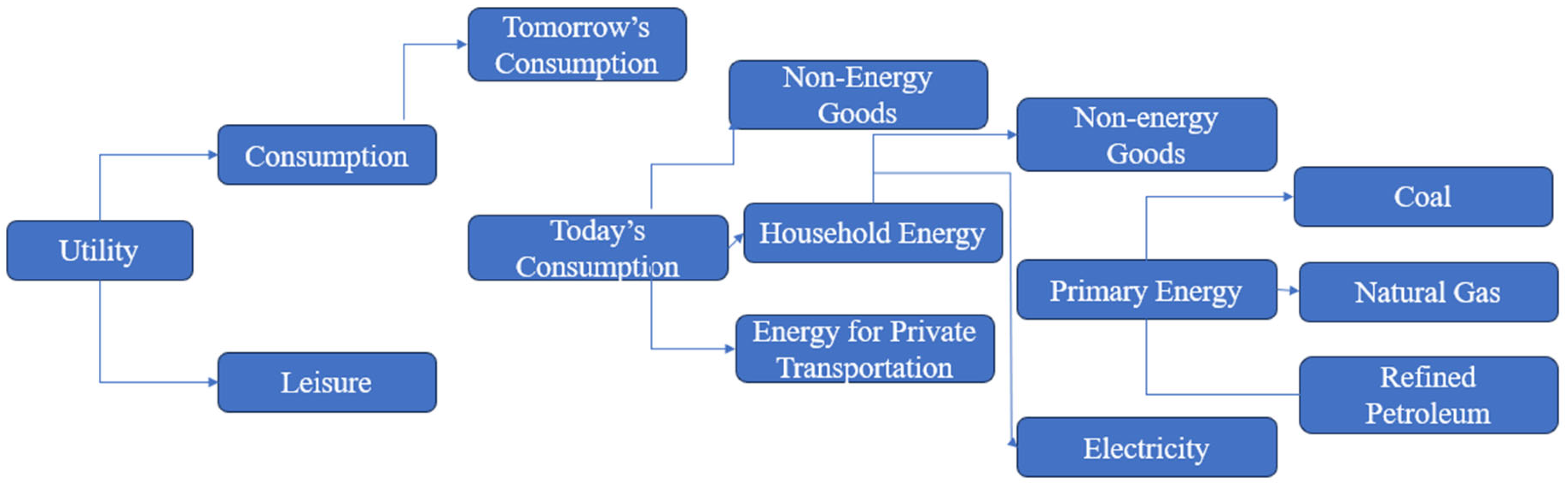
Figure 1 illustrates how households distribute their consumption across different categories, including leisure, energy for private transport, electricity, and non-energy goods, each of which contributes to emissions in different ways.
The biggest drivers of household carbon emissions tend to be transportation, housing, and food [
26,
27]. It is important to distinguish between different types of energy used in households [
28]. Electricity is essential for various household activities such as lighting, cooling, cooking, cleaning, and heating. Coal, natural gas, and petroleum products, on the other hand, have more specific uses, mainly for heating and transportation. Research by [
29] found that these three categories are responsible for around 75% of total emissions, which increases to 85% when leisure activities are included. Similarly, ref. [
27] examined the carbon footprint of an average US household based on five categories and further divided them into direct and indirect emissions. Their study confirmed that transportation, housing, and food contribute the most to household emissions, with fuel consumption being the largest direct source (about 20% of total emissions), followed by electricity consumption (15%) and meat consumption (5%).
Additionally, demographic factors influence household energy use and overall carbon footprints. Studies based on household surveys indicate that factors such as housing type, energy consumption, family size, age, education level, and marital status of the household head all affect emissions differently [
21,
22,
30,
31,
32,
33,
34,
35,
36,
37,
38,
39,
40,
41].
2.1. The Determinants of Household Carbon Footprints
A key determinant of the carbon footprint is household income (total household expenditure is often used as a proxy for income, as total household expenditure is generally more accurately captured in surveys than income). Carbon footprints generally tend to increase with rising income levels [
4,
28,
42,
43,
44,
45]. Weber and Matthews (2008) [
44,
46] emphasize that households with higher incomes or total expenditures tend to exhibit greater variation in their carbon footprints. However, [
47], in a comparative study of four countries, found exceptions to this trend, noting that lower-income households derive a larger share of their carbon emissions from direct energy consumption compared to wealthier households. While this pattern was observed in the UK and The Netherlands, contrasting trends were identified in other regions.
2.2. The Household Welfare Model
Household welfare
is a function of household disposable income
adjusted by equivalence scales
to account for household size and composition. Equivalence scales modify household income to account for variations in size and composition, providing a more accurate indicator of economic well-being. The selection of an equivalence scale significantly influences evaluations of inequality and poverty levels.
Equivalence scale-adjusted income serves as a measure of household welfare, enabling meaningful comparisons of well-being across households with varying sizes and compositions.
Disposable income
is a function of employment income
, other income
, benefits
, and taxes
:
A vector of carbon intensity of each monetary unit of industrial production.
The carbon intensity of industry output represents the amount of carbon emissions produced per unit of monetary output in different industries. This vector helps measure the environmental impact of economic activities by linking industry production to emissions. It is commonly used in input/output analysis to assess the indirect carbon footprint of consumption and production processes. Let C be the carbon intensity vector (carbon emissions per unit of industry output), where each
element represents the carbon emissions per monetary unit of output in industry
i. E denotes the vector of total emissions, where Eᵢ represents the total emissions from industry
i. Let X be the vector of total output, where Xᵢ corresponds to the total monetary output of industry
i. The carbon intensity vector can then be expressed as:
where each element is calculated as:
This approach determines emissions intensity per unit of output and is commonly applied in input/output analysis to estimate indirect emissions associated with both consumption and production.
2.3. Carbon Emissions Factors by Fuel Type
Each type of fuel has a unique emissions factor determined by its chemical makeup and energy content, typically measured in tCO2/kWh. Biomass fuels like firewood are considered carbon-neutral if harvested sustainably. Among fossil fuels, coal has the highest carbon intensity due to its high carbon content and lower energy efficiency, while natural gas has the lowest, owing to its high hydrogen-to-carbon ratio. Diesel emits slightly more carbon than petrol because of its higher energy density. The carbon intensity of liquid fuels varies based on their composition and refining methods.
2.4. Total Emissions vs. Emissions Intensity
Distinguishing between total emissions and emissions intensity (emissions per unit of income) is essential for analyzing the distributional effects of carbon pricing. Total emissions represent the overall volume of greenhouse gases emitted, often linked to the scale of economic activity or energy use. In contrast, emissions intensity reflects the relative emissions burden in relation to income, revealing how carbon costs impact households and businesses across different income levels. Lower-income groups typically allocate a larger portion of their income to energy and carbon-intensive goods. As a result, despite having lower total emissions, they experience higher emissions intensity. This disparity means that carbon pricing policies tend to place a heavier financial burden on these groups, making emissions intensity a critical metric for evaluating distributional impacts and designing fair mitigation strategies.
2.5. Energy Intensity of Household Consumption
Household energy intensity, defined as energy consumption per unit of expenditure or income, plays a key role in evaluating the distributional effects of energy and carbon pricing policies. Lower-income households tend to have higher energy intensity since essential energy costs, such as heating, electricity, and transportation, make up a larger share of their total spending. Conversely, while higher-income households may consume more energy in absolute terms, energy accounts for a smaller proportion of their overall expenditures.
2.6. Heating Fuel Mix and Household Energy Costs
The mix of heating fuels—the blend of energy sources used for residential heating—significantly influences both household energy expenses and the distributional impact of carbon pricing. The cost of domestic energy per kWh is a crucial factor in determining energy affordability and how carbon pricing affects different income groups.
2.7. Effective Carbon Rates (ECR) Across Sectors and Fuel Types
Effective Carbon Rates (ECR), measured in currency units per ton of CO
2 emitted (tCO
2), vary across sectors and fuel types based on the OECD’s Effective Carbon Rates analysis. This framework classifies emissions by sector, including agriculture and fisheries, buildings, electricity, industry, off-road, and road transport, while also breaking down carbon pricing by fuel type, such as coal, fuel oil, kerosene, natural gas, diesel, gasoline, LPG, and other fossil fuels [
20].
2.8. Direct Carbon Emissions from the Household Consumption
Direct carbon emissions from household consumption arise from activities such as burning fuels for heating, cooking, and personal transportation. These emissions are directly tied to household energy choices, including the use of electricity, natural gas, and fuels like gasoline or diesel.
In an input/output (IO) model, direct household emissions are estimated by applying emission factors to the final demand vector corresponding to household consumption. Specifically, emissions from each household activity are calculated by multiplying household expenditures on energy-intensive goods (represented in the final demand vector f) by the direct emissions intensity for each sector (e). The total direct emissions where e is the direct emissions intensity vector that quantifies emissions per unit of output in each relevant sector, such as energy production, transportation, and heating. This formulation helps assess the direct carbon footprint of households and can guide policies aimed at reducing energy consumption and promoting cleaner technologies.
2.9. Indirect Carbon Emissions from Household Consumption
Indirect carbon emissions stem from the production, transportation, and supply chain activities associated with the goods and services households consume. Although these emissions occur outside the household, they are driven by consumption choices.
To estimate indirect emissions, input/output (IO) models are commonly used, as they track carbon flows across different industries and capture the economic interconnections between sectors. This framework helps quantify the broader environmental impact of household consumption by considering emissions embedded in the production and distribution of goods and services. To estimate indirect carbon emissions from household consumption, we use an environmentally extended input/output (EEIO) model. Let E represent the vector of total sectoral emissions, A the technical coefficients matrix, and y the final demand vector representing household consumption. The Leontief inverse matrix, accounts for both direct and indirect effects across industries.
2.10. Decomposing the Distributional Impact of Carbon Taxation
The economy-wide emission intensity per unit of final demand, where γ is a row vector representing total emissions per unit of final demand; is the direct emissions intensity vector (1xn), where represents emissions per unit of output for sector i.
The total indirect carbon emissions from household consumption are:
E is the total indirect carbon emissions from household consumption. The total emissions associated with household consumption can then be formulated as:
If disaggregated by household groups (e.g., by income deciles), household-specific final demand vectors can be used to compute emissions for different household types.
Decomposing the distributional impact of carbon taxation.
Disposable income
after a carbon tax (
):
= savings rate;
= “budget share of household expenditure allocated to expenditure group i”;
= carbon intensity of expenditure category i expressed in t of CO2 per unit (kWh for energy goods2 and EUR for non-energy goods);
= price per unit of energy paid by household ℎ;
= indicator variable ⟶ household owns a carbon-emitting asset;
= carbon price per ton of CO2.
Equation (6) provides a framework for analyzing the distributional impact of carbon taxation by considering key drivers of household carbon emissions. One primary driver is household expenditure patterns, captured by the budget share . Households that allocate a higher proportion of their spending to energy-intensive goods and services will experience a greater reduction in disposable income due to carbon taxation. Another significant driver is the carbon intensity of consumption , which varies by expenditure category. Energy goods, such as electricity and heating fuels, have higher direct carbon intensities, whereas non-energy goods contribute indirectly through supply chain emissions. The price per unit of energy further influences emissions, as households paying higher energy prices may be more incentivized to reduce consumption or switch to cleaner alternatives.
Household characteristics, such as ownership of carbon-emitting assets , also shape emission levels. Households that own vehicles, use private transportation, or rely on fossil fuel-based heating systems will face a higher tax burden compared to those using cleaner technologies. Additionally, income and savings behavior play a role, as lower-income households tend to spend a larger share of their income on energy and have limited flexibility to adjust consumption in response to carbon price increases . This makes carbon taxation potentially regressive unless offset by revenue recycling or targeted support.
3. Methodology and Data
To capture the full impact of carbon emissions, we must account for both direct emissions and indirect emissions. This requires an input/output (IO) framework to trace emissions across the production chain. To assess the distributional effects of carbon pricing, Household Budget Survey (HBS) data provide valuable insights into how different income groups are impacted. By integrating these data with emissions estimation simulations, an input/output (IO) framework for indirect effects, and micro-level analysis to examine distributional impacts, we can create a thorough evaluation of how carbon pricing influences households across income levels.
The present study employs the PRICES (Prices, Revenue Recycling, Indirect Taxation, Carbon, Expenditure Simulation) microsimulation model [
33,
48], which is specifically designed to evaluate the distributional and environmental impacts of price and tax changes at the household level. The model is well-suited for analyzing carbon emissions and energy use because it captures the heterogeneity of household consumption patterns and links these to both fiscal and environmental policy instruments. This is particularly important in middle-income countries such as Türkiye, where income inequality, energy insecurity, and consumption diversity complicate the impact assessment of carbon pricing. PRICES simulates the effects of price increases arising from various sources, including external inflation shocks, indirect tax reforms, and environmental levies such as carbon taxes. Using detailed household budget survey data allows fine-grained, disaggregated analysis across income groups, regions, and household characteristics, thereby providing insights into both vertical (across income levels) and horizontal (within income groups) equity.
Crucially, the model incorporates two approaches for estimating CO
2 emissions at the sector level, offering methodological flexibility. The first approach uses emissions intensity vectors from [
49], which include both process and fugitive emissions, enabling a broad, economy-wide view. The second approach focuses solely on energy-related emissions derived from sector-level energy consumption data. This is particularly useful for simulating carbon taxes on energy use, which is central to the present study. The use of PRICES is justified by its ability to capture heterogeneity in household behavior and energy use, to model carbon pricing effects realistically in a country-specific context using national-level data, and to simulate policy alternatives such as revenue recycling and targeted transfers, which are critical for assessing equity outcomes.
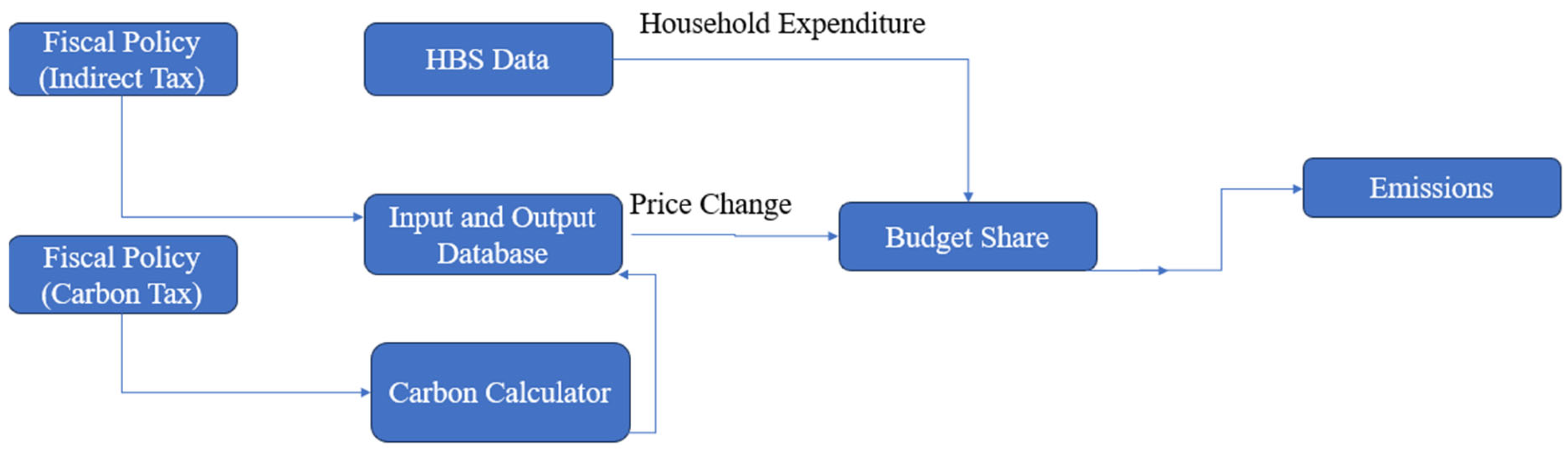
The PRICES microsimulation model is structured as illustrated in
Figure 2.
The methodological framework (
Figure 2) contains the following:
- -
Household Budget Survey (HBS) data [
24], which captures consumption patterns and expenditure shares, enabling the assessment of fuel expenditures and the calculation of direct carbon emissions [
51,
52].
- -
The input/output (I-O) database links sectoral economic data to household spending, estimating how price changes from fiscal policies, such as indirect and carbon taxes, impact expenditures.
- -
Ultimately, changes in income and prices shift consumption patterns and influence emissions, reducing CO2 output.
- -
Our econometric approach and proposed model are based on [
25,
53].
Data
The Household Budget Survey (HBS) 2019 was chosen over the Survey on Income and Living Conditions (SILC) because it provides detailed household expenditure data, which is essential for analyzing carbon pricing impacts and distributional effects. Due to the significant disruptions caused by the COVID-19 pandemic and the subsequent Russia–Ukraine conflict, the 2019 data have been identified as the most reliable baseline for analysis. The HBS is essential for analyzing consumption-based carbon emissions and the distributional effects of carbon pricing. Household Budget Survey (HBS) datasets provide detailed information on household expenditures by item, along with demographic, socioeconomic, and income data. The analysis uses the Turkish Household Budget Survey (HBS), collected by Statistics Turkey in 2019. To examine inter-industry relationships, the model incorporates the 2016 World Input-Output Database (WIOD) and its environmental extension, which includes industry-specific CO
2 emissions data [
54].
The focus of the analysis is on household consumption expenditure (as defined by [
55] to assess consumption-based carbon footprints (CF). A common approach for analyzing household CF is to combine HBS data with greenhouse gas (GHG) emissions intensities, as conducted in several countries, including Finland (e.g., [
56]), Norway [
57], Germany [
58]. Environmentally extended input/output (EEIO) models are frequently used to estimate consumption-based emissions intensities (e.g., [
59]) and have been applied to evaluate impacts and prioritize policy measures to reduce GHG emissions and model lifestyle changes [
7,
60].
Input/output (IO) models and multiregional input/output (MRIO) models can be extended with environmental extensions to track the environmental impact of production processes across global supply chains. This leads to the development of environmentally extended input/output models (EEIO). These extensions account for emissions or resource use linked to the production activities of various sectors across different regions. In the case of carbon emissions, EE-IO models create a connection between products and the indirect carbon emissions embedded in the production of goods and services. [
61] presented an ecologically extended input/output analysis, while Minx et al. (2009) [
62], ref. [
63] outlined its applications in estimating carbon footprints. It provides a valuable tool for analyzing changes in household consumption patterns, as shaped by national production technologies and emission intensities, and helps examine how income, demographics, and lifestyles influence variations in HCFs.
To model the indirect effects of producer price changes and carbon taxes, the pass-through of price changes to households is captured using an input/output (IO) table. Originally developed by Leontief (1951) [
64] and further refined by Miller and Blair (2009) [
65], IO modeling has been used in earlier studies such as [
40] in Ireland, [
58] in the United Kingdom, and [
66] to analyze the distributional effects of carbon taxation. More recent developments in distributional impact analysis, such as those by Sager (2019) [
48] and Feindt et al. (2021) [
6,
34,
55], use multiregional IO (MRIO) models to further refine these assessments.
The central equation of our IO model, a Leontief quantity model, is the
Leontief inverse matrix , where
is the identity matrix and
is the technology matrix. The Leontief inverse gives the direct and indirect inter-industry requirements for the economy:
where
is a vector of final demand.
Transforming an IO model into an EE-IO requires a carbon intensity vector, capturing carbon emissions emitted by the industry in the production of a monetary unit of its output [
67]. Multiplying the Leontief inverse with the carbon intensity vector, we obtain a vector of the carbon intensity of each monetary unit of industrial production (
, accounting for emissions released by the industry and by all downstream industries [
51]. Using bridging matrices, we can translate the carbon emissions associated with industry outputs into indirect emissions associated with products consumed by households
. To compute total household-level emissions, we combined information on household fuel consumption with the carbon intensity of each fuel to create a vector of the household’s direct carbon emissions (
The sum of direct and indirect emissions gives households’ total carbon emissions associated with their consumption (
:
Total emissions can be written as the product of the emission intensities per EUR multiplied by the total expenditure for a given consumption category
c,
where
is a vector of (in-)direct emission intensities, expressed in kilograms of CO
2 equivalent emissions per EUR spent (kg CO
2e/EUR),
is a matrix of household expenditures (in EUR) for each household, capturing their associated spending patterns. This formulation allows for the calculation of household-level carbon footprints by linking emission intensities with specific expenditure data, enabling a detailed analysis of the environmental impact of consumption behaviors.
This study estimates household carbon footprints by combining Household Budget Survey (HBS) data with the World Input-Output Database (WIOD), mapping household consumption expenditures to emissions at the industry level. Since HBS follows the Classification of Individual Consumption by Purpose (COICOP) and WIOD utilizes ISIC rev. 4 or NACE rev. 2, a bridging matrix is necessary to connect consumption categories to industry outputs [
68]. For a more detailed explanation, refer to [
18,
54,
69].
4. Results
This section analyses household carbon emissions and energy consumption across income deciles, focusing on distributional impacts and energy affordability. It examines carbon emissions by fuel type, energy use and intensity, and domestic energy pricing and taxation. The results highlight differences in energy costs, tax burdens, and budget shares, showing how energy expenses affect households across income groups. Additionally, the comparison of direct and indirect emissions per expenditure provides insights into household carbon footprints and the equity implications of carbon pricing policies.
Different fuels have different carbon emissions depending upon their chemical structure. Different fuels emit varying amounts of carbon dioxide (CO
2) depending on their chemical composition and combustion characteristics. According to the Intergovernmental Panel on Climate Change, coal has the highest carbon intensity, releasing approximately 90–100 kg of CO
2 per gigajoule (GJ) due to its high carbon content. Oil-based fuels, such as gasoline and diesel, emit less, typically around 70–75 kg CO
2/GJ, while natural gas, which consists primarily of methane (CH
4), has the lowest carbon intensity among fossil fuels, emitting approximately 50–55 kg CO
2/GJ. Biofuels, depending on their production process, may have lower net emissions due to carbon sequestration during biomass growth. The differences in carbon emissions across fuels play a crucial role in shaping climate policies and energy transition strategies [
70].
Figure 3 illustrates that firewood has the highest carbon emissions per kWh among the fuels listed. While it is often considered a renewable resource, its high carbon emissions highlight the impact of inefficient burning and potential deforestation. Coal follows as the second-highest emitter, aligning with its reputation as a major contributor to global carbon emissions and reinforcing the push toward phasing out coal in favor of cleaner energy sources. Among fossil fuels, diesel, petrol, and liquid fuel show moderate emissions, with diesel being higher, often due to its use in industrial and heavy transportation sectors. Petrol, commonly used in transportation, has lower emissions than diesel and liquid fuel. Natural gas stands out as the lowest emitter among conventional fuels. It is often promoted as a transition fuel toward greener energy because of its relatively lower carbon footprint; however, methane leaks during extraction and transportation could undermine these benefits.
Analyzing carbon emissions by fuel type is necessary for designing effective, equitable, and targeted climate policies. It enables a better understanding of emission sources, helps identify distributional impacts, and supports the development of fuel-specific decarbonization strategies to achieve both environmental and social policy goals. Energy costs place a heavier financial burden on lower-income households.
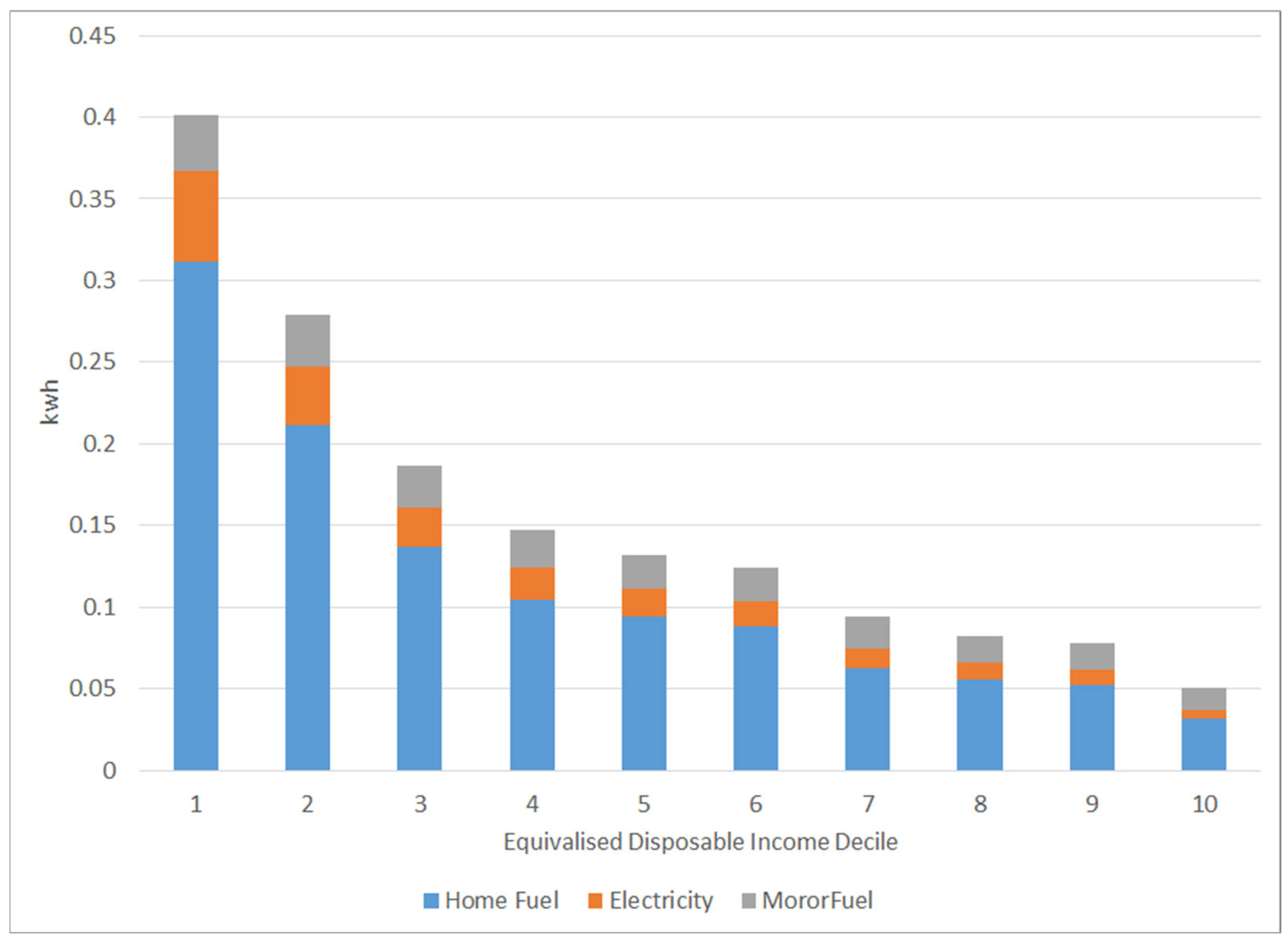
Figure 4 highlights that lower-income deciles (1–3) exhibit higher energy intensity, meaning they use a larger proportion of their income on energy compared to higher-income groups. As income rises, the share of income spent on energy decreases, showcasing a falling share of income allocated to energy needs. The burden of energy costs is not equally distributed, as lower-income groups spend proportionally more on essential energy needs like home fuel and electricity, while higher-income groups have a greater proportion of their energy consumption in the motor fuel category, indicating more discretionary or mobility-related energy use.
Understanding the distributional impact of energy use is essential for developing policies that promote both equity and sustainability.
Figure 5 illustrates the distributional impact of energy intensity, showing the ratio of energy consumption (kWh)-to-income across income deciles. The chart reveals an inverse relationship between income and energy intensity, with lower-income households (Decile 1) exhibiting significantly higher energy intensity. The high energy intensity in Decile 1 is primarily driven by home fuel consumption, followed by electricity and motor fuel, indicating that a large portion of their limited income goes toward basic energy needs. As income increases from Decile 2 to Decile 10, energy intensity decreases sharply. Higher-income groups consume more energy in absolute terms but allocate a smaller share of income to energy, reflecting their economic resilience. The blue segment (home fuel) dominates across all deciles but is most significant for lower-income groups, highlighting their reliance on energy for heating. Motor fuel (grey) becomes more prominent in middle-income deciles, reflecting greater mobility needs, while its share remains modest in higher-income deciles due to more energy-efficient transport options.
Addressing energy affordability and its impact on household budgets is crucial for fostering a fair and sustainable energy transition.
Figure 6 illustrates the energy intensity of household consumption across income deciles, measured in kilowatt-hours (kWh) per unit of income. The chart highlights how lower-income households (Decile 1) have significantly higher energy intensity, meaning they spend a larger share of their income on energy consumption compared to wealthier households. As income increases, energy intensity declines, with the highest-income deciles (Decile 10) exhibiting the lowest energy usage relative to their income.
The chart categorizes energy consumption into three components:
- -
Home Fuel (Blue): The dominant component, representing heating fuels like gas, coal, or wood.
- -
Electricity (Orange): Covers household electricity consumption for appliances, lighting, and other uses.
- -
Motor Fuel (Gray): Includes fuel used for personal transportation.
The figure reveals a regressive pattern, where low-income households bear a disproportionately higher energy burden. This suggests that energy cost policies, such as carbon taxes or subsidies, may have significant equity implications, particularly for vulnerable households.
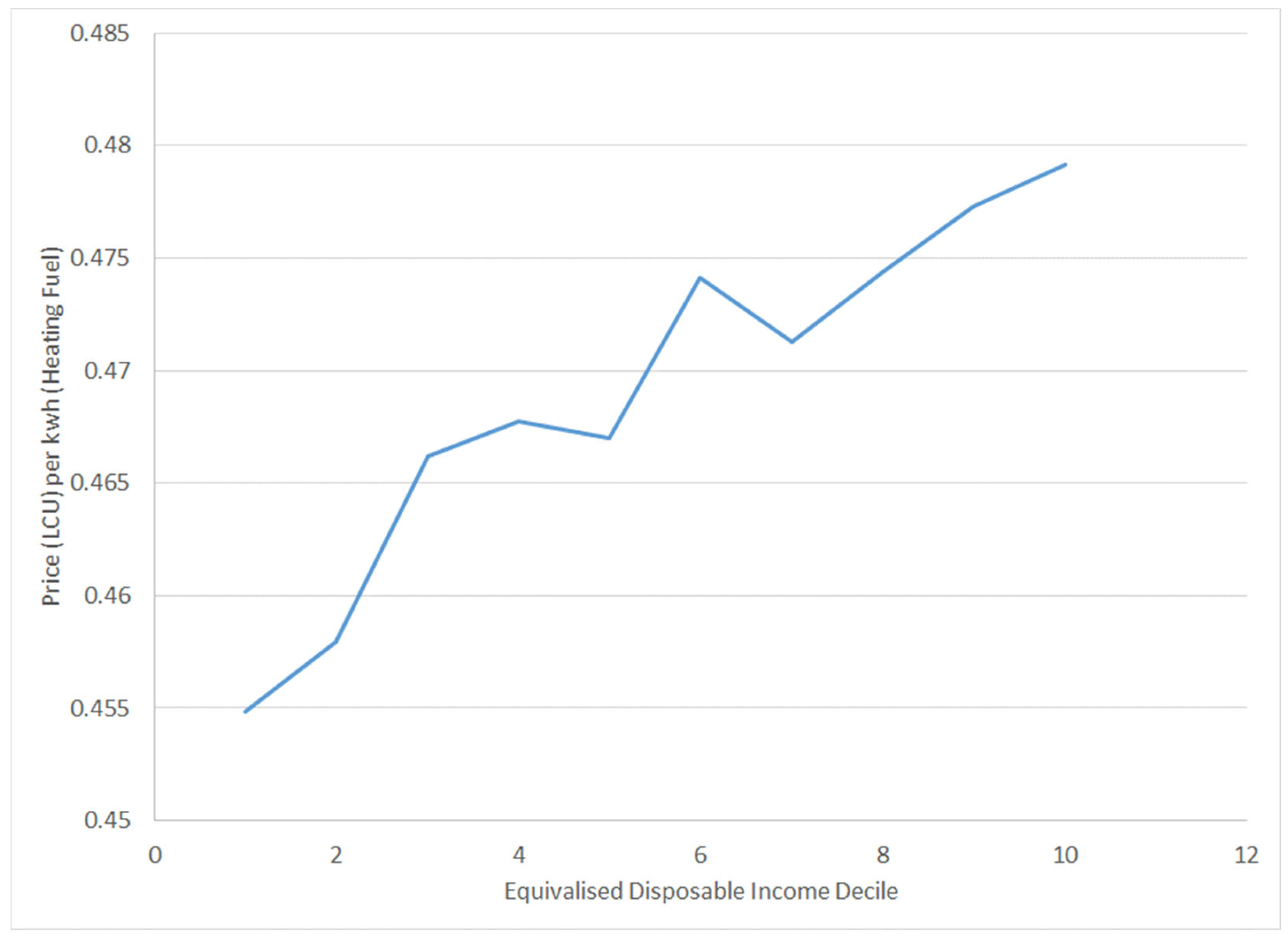
Understanding the price of domestic energy per kWh across different equivalized disposable income deciles, as shown in
Figure 7, is important for several reasons. It helps identify how energy costs are distributed across income groups and whether lower-income households pay higher prices for energy.
Figure 7 shows that lower-income households (on the left side) pay more per kWh for heating fuel than higher-income households (on the right side). The price generally decreases as income increases, with some fluctuations in the middle deciles. This indicates a regressive pricing structure, where poorer households face a higher cost burden for energy, highlighting the need for more equitable pricing policies.
Effective Carbon Rates (ECRs) are essential for reflecting the true cost of carbon emissions, driving businesses and consumers to reduce their carbon footprint. By comparing ECRs across fuels and sectors, policymakers can identify carbon pricing gaps and craft fairer, more efficient environmental tax policies.
Figure 8 illustrates the Effective Carbon Rates across various sectors and fuel types, measured in currency units per ton of CO
2 emitted (tCO
2), based on the OECD’s Effective Carbon Rates (ECR) analysis. It categorizes emissions by sectors such as agriculture and fisheries, buildings, electricity, industry, off-road, and road, and breaks down carbon rates by fuel types, including coal, fuel oil, kerosene, natural gas, diesel, gasoline, LPG, and other fossil fuels.
Figure 9 presents the budget share allocated to energy expenditures across different income deciles, with a focus on heating and electricity, motor fuel, and the ratio of home energy-to-motor fuels.
The x-axis represents equivalised expenditure deciles, ranging from the lowest (1st decile) to the highest (10th decile), while the left y-axis shows the budget share, and the right y-axis indicates the ratio of heating and electricity-to-motor fuels. The solid red line indicates the budget share for heating and electricity, the dashed red line represents motor fuel expenses, and the blue line shows the ratio of home energy-to-motor fuels. Key observations include the following:
- -
Home Energy Concentration: The budget share for heating and electricity is significantly higher in the lowest income deciles, indicating that domestic fuel expenses are more concentrated at the very bottom of the income distribution.
- -
Motor Fuel Profile: The budget share for motor fuels (dashed red line) is relatively flat in the middle of the income distribution, suggesting a more consistent expenditure pattern across these deciles.
- -
Ratio of Home Energy-to-Motor Fuels: The blue line, showing the ratio of heating and electricity expenses-to-motor fuel costs, declines as income increases. This suggests that lower-income households allocate a much higher proportion of their energy budget to home heating and electricity than to motor fuels, compared to higher-income households.
Overall, the visualization highlights the regressive nature of home energy costs, with lower-income households facing a disproportionately high burden from heating and electricity expenses. Meanwhile, motor fuel expenses appear more evenly distributed across the middle-income deciles. The declining ratio of home energy-to-motor fuels with rising income further underscores the greater sensitivity of lower-income households to domestic energy costs.
Income-based disparities in spending patterns show how lower-income households allocate a much larger share of their income to essential goods like food and energy.
Figure 10 shows the share of income spent on food, energy, and other expenses across income deciles. The lowest-income households (Decile 1) spend a significantly larger share of their income on necessities than higher-income groups, making them more vulnerable to indirect taxation or price increases. As income rises, the proportion spent on essentials declines, reflecting greater financial flexibility among wealthier households. While energy costs (orange) are a smaller share overall, they remain a burden for low-income groups. Policy measures like carbon pricing or energy taxes could disproportionately affect lower-income households unless offset by subsidies or targeted transfers. Understanding these spending patterns is crucial for designing fiscal and environmental policies that avoid worsening inequality.
Figure 11 highlights the distributional impact of carbon emissions across income groups, showing that direct emissions vary slightly with income, while indirect emissions are relatively constant. In
Figure 1, the blue line shows direct emissions from household energy use (fuel, heating, electricity), and the orange line represents indirect emissions embedded in goods and services (food, transport, manufactured goods). Direct emissions increase slightly with income, peaking in the middle deciles before declining at the highest levels, whereas indirect emissions remain relatively stable across all income groups. Higher-income households tend to produce more direct emissions due to greater energy consumption, such as larger homes and more vehicle use. This suggests that carbon pricing and energy taxes may have unequal effects across income groups, with higher-income households contributing more to direct emissions while indirect emissions remain consistent across all deciles.
The graph aims to show how carbon pricing policies (like taxes or emissions trading) affect households at various income levels.
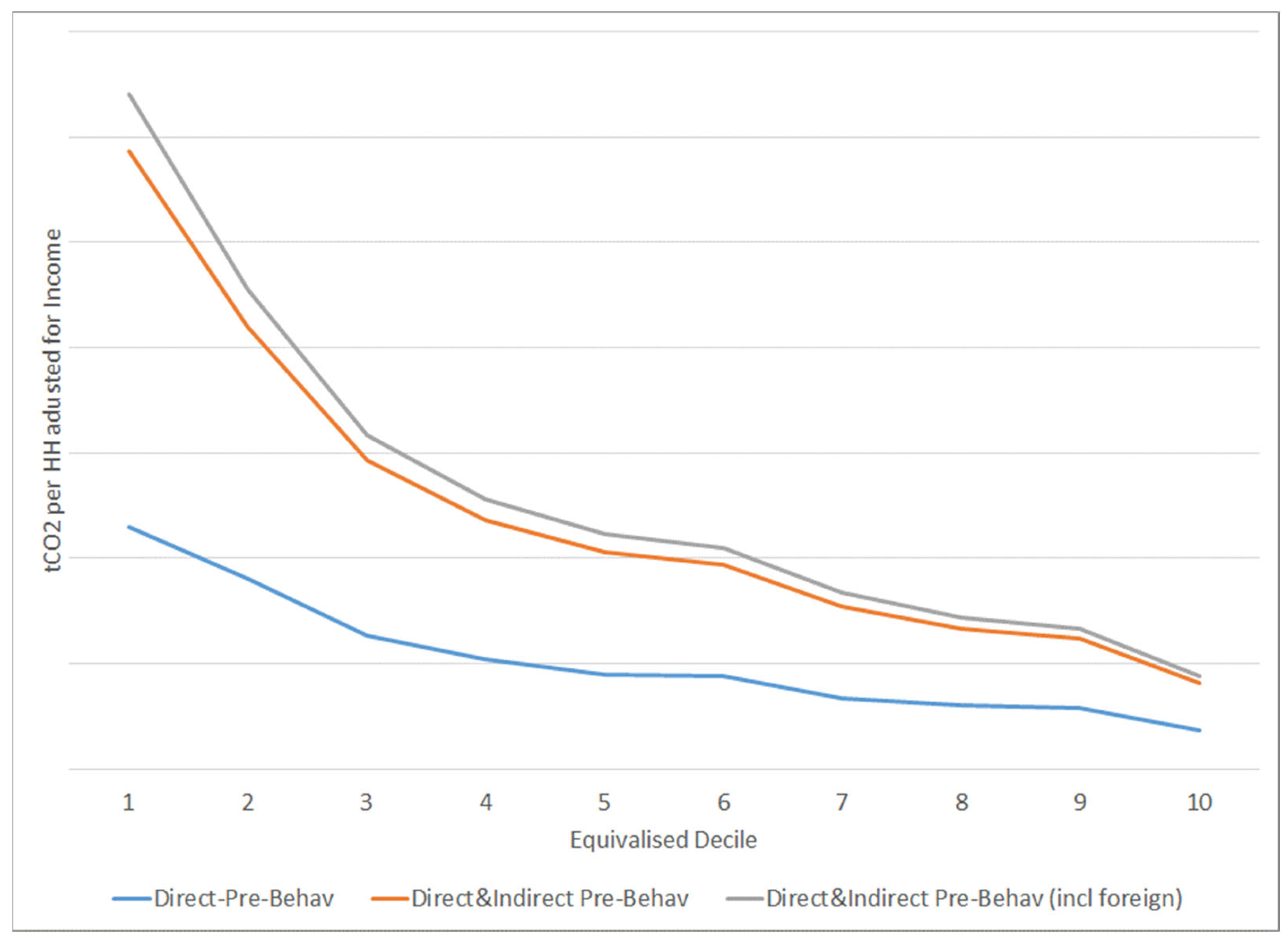
Figure 12 illustrates the carbon emissions per household expenditure, distinguishing between direct and indirect emissions across income deciles. The y-axis represents tons of CO
2 per household (adjusted for income), while the x-axis shows equivalized income deciles from the lowest-income group (Decile 1) to the highest-income group (Decile 10).
The analysis of household emissions across income deciles reveals distinct patterns. Direct emissions (blue line) from fuel use, such as heating and transportation, are most intense in lower-income households (Decile 1) and decrease with higher income. Including indirect emissions (orange line) from goods and services, the trend remains similar, with intensity declining across deciles. When foreign supply chain emissions (gray line) are added, higher-income deciles show increased emissions due to greater consumption of imported goods. This highlights the regressive nature of energy taxation on lower-income households and the global impact of consumption-driven emissions in wealthier deciles. Policymakers must design targeted interventions to address these disparities, balancing direct and indirect carbon footprints while considering the broader implications of consumption patterns. Lower-income households have higher emissions per unit of expenditure, largely due to a greater reliance on carbon-intensive fuels for essential needs. Higher-income households have lower emissions per unit of expenditure but contribute more to total emissions, particularly through indirect and foreign-related emissions. This suggests that carbon pricing policies need to consider both direct household energy consumption and indirect emissions from consumption patterns, particularly in wealthier households.
5. Discussion and Conclusions
This study explores the distributional drivers of carbon emissions in Türkiye, revealing the nuanced ways household income influences both the level and type of emissions. A key finding is an inverse relationship between income and energy burden. Lower-income households spend a larger share of their income on essential energy needs, making them more vulnerable to carbon pricing, while higher-income households—though less energy-burdened—contribute disproportionately to indirect emissions through consumption of energy-intensive and imported goods.
Importantly, the study distinguishes between direct emissions from domestic energy use and transport and indirect emissions embedded in the supply chains of goods and services. This dual-emission structure suggests that effective carbon mitigation requires comprehensive strategies that go beyond targeting fuel consumption and also address consumption patterns among the affluent.
One of the more innovative insights is that rising middle classes in countries like Türkiye could significantly shift national carbon footprints, not only through increased energy demand but also through changing consumption behaviour. Therefore, policies should pre-emptively address this evolving dynamic through investment in clean infrastructure, energy efficiency, and sustainable mobility.
To ensure fairness in carbon pricing, targeted compensatory measures, such as energy subsidies, income support, or retrofitting programs, are essential to prevent regressive outcomes. Simultaneously, progressive measures aimed at curbing high-consumption lifestyles and encouraging green consumption are crucial for long-term impact. In sum, climate policy must be both socially equitable and structurally comprehensive to achieve emission reductions without undermining vulnerable populations.
In conclusion, by addressing both direct and indirect emissions and tailoring interventions to the needs of different income groups, it is possible to reduce carbon emissions significantly while promoting social equity and economic resilience. Policymakers in Türkiye can use these insights to develop more equitable and effective carbon pricing strategies that support both environmental and social goals.
6. Contributions and Limits
This research provides valuable insights into the distributional dynamics of carbon emissions in Türkiye and offers great value to policymakers, environmental economists, and social justice advocates. The study shows how household income levels influence both direct and indirect carbon emissions, helping to design targeted carbon pricing strategies that are both environmentally effective and socially equitable. The findings are particularly relevant for middle-income countries experiencing rapid economic growth and changing consumption patterns, as they highlight the need for policies that address the particular challenges of such transitions.
However, the scope of the study is limited by the fact that it is based on data from 2019, which was selected for its stability before the disruptions caused by the COVID-19 pandemic and the Russia–Ukraine conflict. While this provides a solid baseline, it cannot fully capture the current dynamics of household energy consumption and emissions. In addition, the analysis does not take into account behavioral responses to carbon pricing that could influence the effectiveness of the proposed policy measures.
The research objectives—investigating the relationship between household income distribution and carbon footprint and understanding how consumption patterns affect emissions—are thoroughly addressed by applying the PRICES microsimulation model. This methodological approach allows for a nuanced analysis of both direct and indirect emissions across income groups, which is very much in line with the objectives of the study.
In terms of literature contribution, the study fills a notable gap by focusing on the distributional impacts of carbon emissions in a middle-income country context, an area previously underexplored. Its integration of detailed household expenditure data with input/output analysis offers a novel perspective on the interplay between income levels and emission types. This approach not only enhances the understanding of carbon emission drivers in Türkiye but also provides a framework that can be adapted to similar economies facing comparable challenges.


