Spatial Accessibility Characteristics and Optimization of Multi-Stage Schools in Rural Mountainous Areas in China: A Case Study of Qixingguan District

Abstract

Optimizing the allocation of basic educational facilities in mountainous rural areas is important for narrowing the education gap between urban and rural areas, constructing high-quality regional education systems, and achieving sustainable education development. This paper considered preschool, primary, and secondary schools in Qixingguan District, which is located in a mountainous area of China, using vector data of rural residential areas and educational facility points as a source of information on supply and demand. The study combined travel modes and acceptable time of rural school-age population, and applied the Gaussian two-step mobile search method to calculate the level of accessibility of basic educational facilities at the scale of residential areas. Location optimization and scale optimization models were used to determine the optimal location and service qualities for basic educational facilities. Our results yielded three main conclusions. First, the spatial pattern for the distribution density and accessibility of basic educational facilities in Qixingguan differed at all stages, but all of them showed a strong orientation toward the central urban area. Service capacity in each stage tended to extend toward the northeast and southwest, except for a certain orientation toward the central urban area. Second, the main reason for the low spatial accessibility of schools was that the density and service capacity of the available schools did not align with the distribution of the school-age population. Third, after optimizing for location and service capacity, schools at all stages shifted to the northeast of Qixingguan, which reduced the difference in service capacity between schools and improved the accessibility and balance of schools in the northeast and southwest.

1. Introduction

Education is important for obtaining social, economic, political, and cultural benefits; it is an effective way to disseminate knowledge, promote learning, and encourage innovation. Education can effectively reduce poverty and promote regional development, and it plays an important strategic role in national development [1,2,3]. Relevant studies have shown that education level is closely related to health status [4], personal income [5], employment quality [6], science and technology [7], and economic growth [8], among others, and it also affects the process of regional sustainable development. The United Nations 2030 Agenda for Sustainable Development explicitly sets out sustainable development goals to ensure the equitable distribution of quality education [9,10,11]. In China’s Education Modernization 2035, China places a focus on improving the quality of education, promoting equality in education, and promoting balanced education between urban and rural areas. The report of the 20th National People’s Congress of the Communist Party of China stressed the need to accelerate improvements to the quality and balanced development of compulsory education, as well as the integration of urban and rural areas while optimizing the allocation of regional education resources. Spatial accessibility, by focusing on the spatial allocation of facilities in terms of quantity and quality of supply and demand, can effectively solve the problem of imbalances as well as the mismatch of regional public facility resources [12]. This method has gradually attracted the joint attention of planning scholars and geographers.

Spatial accessibility entails residents’ ability to cross distances to obtain needed resources, and its characteristics are an effective method for measuring spatial equity [13]. Commonly used measurement methods include the gravity model [14] and minimum distance [15], chance accumulation [16], and two-step mobile search methods. Spatial accessibility is widely used in the planning and configuration of public facilities such as park green spaces [17,18], tourist attractions [19], medical services [20], and fire services [21]. The two-step mobile search method considers the supply-demand relationship between residents and resource facilities; this method has been constantly improved to enhance the calculation accuracy for accessibility, leading to refinements such as the two-step mobile search method of kernel density considering distance attenuation [17,22], the gravity two-step mobile search method [23], and Gaussian two-step mobile search method (Ga2SFCA) [18], three-step floating catchment area method [24], among others. The variable two-step mobile search method [25] and dynamic two-step mobile search method [26], which both consider the search radius, provide a rich reference for the measurement of the spatial accessibility of schools, which has been linked to people’s well-being. Scholars have used multi-source spatial-temporal data and analysis methods to fully explore the spatial accessibility characteristics and influencing factors of urban and rural basic educational facilities such as kindergartens [27,28], primary schools [29,30], and middle schools [31]. Based on the evaluation of accessibility, the equilibrium of spatial allocation of schools can be qualitatively and quantitatively analyzed [32]. Because the accessibility of educational resources affects travel costs and travel intention, some scholars have studied the mechanisms through which the accessibility of schools influences academic achievement [33], location value, and housing prices [32,34,35,36], among others, to provide a theoretical reference for the optimization of school distribution.

Optimization of school distribution is a classic geographical problem, and the spatial optimization model is an effective way to solve this problem by allocating the location and scale of schools under constraints to achieve the established objectives [37,38]. This study considers school capacity [39], commuting distance [40], enrollment opportunity [38], and other factors, and constructs an optimization model to minimize inaccessibility [41] and inter-school differences [40] to optimize the distribution efficiency and accessibility of schools. Similar studies have been conducted. For example, Han et al. [42] determined a location-allocation scheme for primary schools in a case district by comparing the minimization impedance model with the maximization coverage domain model. Lotfi et al. [43] constructed a multi-objective optimization model considering population change and provided suggestions for school location in a case district. Cai et al. [44] put forward the urgency of optimization as a concept to determine the optimization order for schools within a region and optimize the location and scale of schools in new urban areas. These studies mainly focused on the spatial distribution of educational needs and the optimal matching of the location of schools, but they seldom optimized the comprehensive scale of schools based on their location optimization.

According to the research results and methods for evaluating and optimizing the accessibility of schools, the spatial location and scale information of the school-age population and schools are an important data foundation for measuring the accessibility of schools. However, current research has tended to express the distribution of the school-age population according to the geometric center of administrative units or blocks [17,38,45]. However, the travel modes of the school-age population in mountainous areas are relatively limited and can be highly biased at different education stages. Previous studies have ignored the travel time willingness of rural students, which can affect the authenticity of the results calculating accessibility. Looking at current conditions, it is urgent to fully consider the travel willingness of the school-age population, optimize the distribution and scale of schools, and improve enrollment opportunities for the school-age population in mountainous areas.

This study considered Qixingguan District, a typical mountainous area in China, and extracted patches of rural settlements through remote sensing interpretation to assess the spatial location of the school-age population. Field research was conducted to determine the duration and mode of travel willingness among the school-age population in mountainous areas. An index system was then constructed to comprehensively evaluate the serviceability of schools; this was followed by the application of Ga2SFCA, location optimization, and scale optimization model, and other methods. This paper evaluated and optimized the spatial accessibility of multi-stage educational facilities in a mountainous area in China to provide a reference for the balanced distribution of educational resources in rural areas, narrowing the urban-rural education gap, and promoting sustainable education development in such areas.

2. Materials and Methods

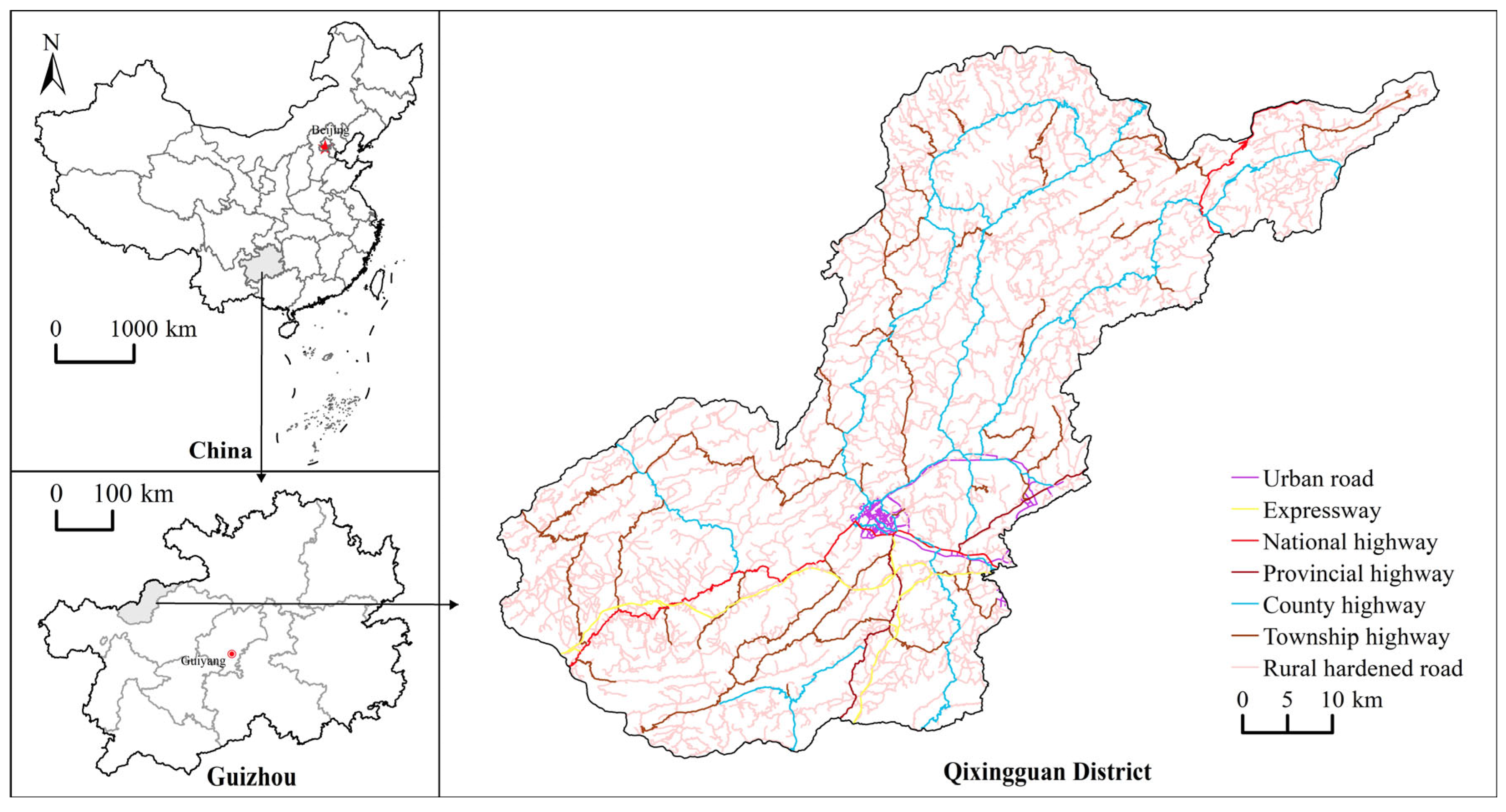
2.1. Study Area

Qixingguan District (Figure 1) is located in Guizhou Province in southwest China, and is one of the key areas for the implementation of China’s western development. Since the implementation of China’s western development, the rate of enrollment rate among school-age children increased from 89% in 2000 to 99.96% in 2018, showing significant achievements in basic education popularization. By 2018, there were 873 basic educational facilities covering preschool education, primary education, and secondary education in the district. The rural school-age population in the region that needs to receive basic education is 412,800 individuals, but the harsh natural and socio-economic conditions in the region, including broken terrain, inconvenient transportation, and lagging economic development, have hindered the construction of schools, the travel of school-age population, and the introduction of teacher resources, exacerbating the uneven distribution of urban-rural educational resources. Therefore, selecting the Qixingguan District as the study area to explore the optimal allocation of rural educational resources can provide case references for sustainable mountainous education development.

2.2. Data Collection and Processing

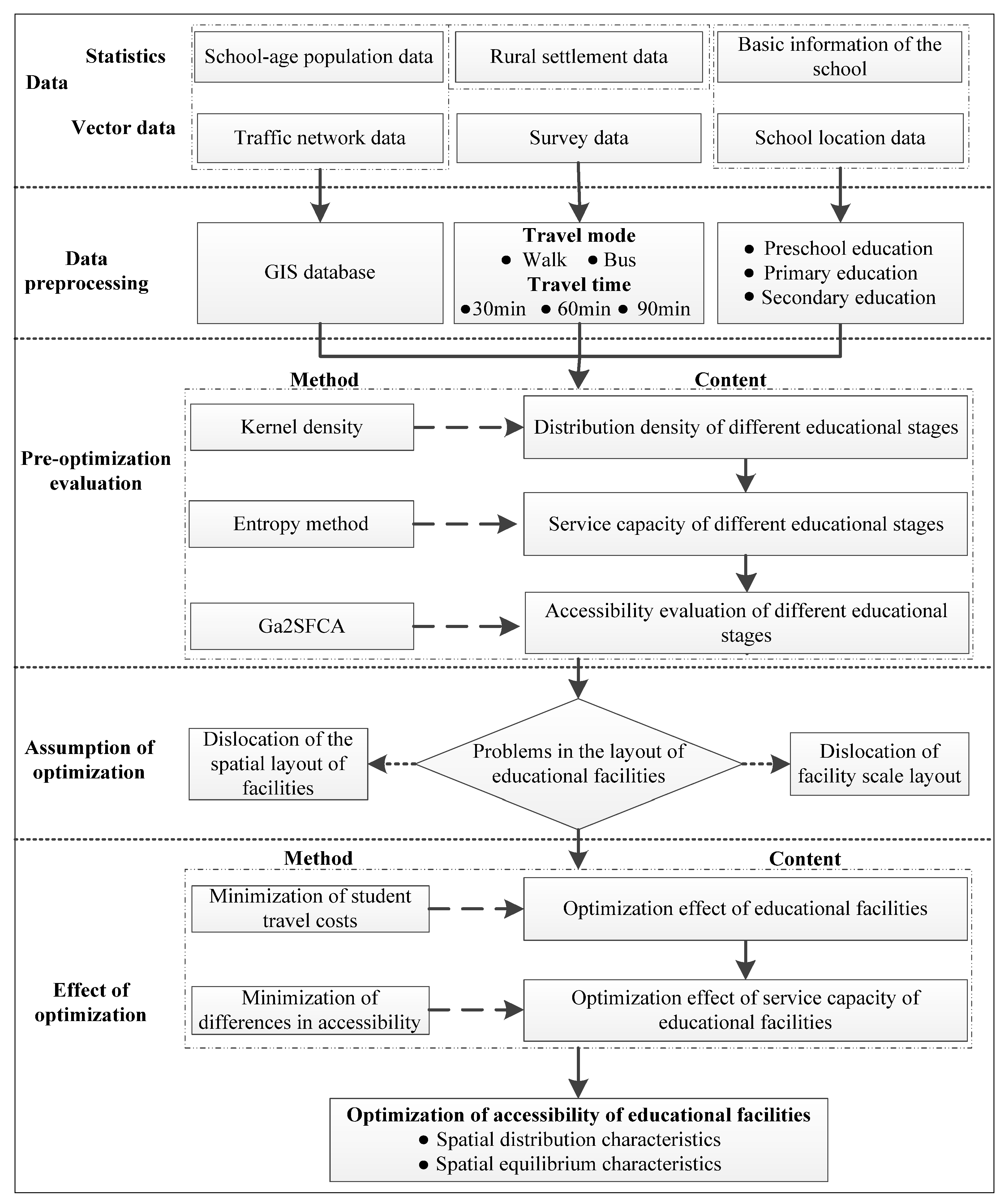
This study primarily involved rural residential data, information on educational facilities at different stages, population data, and traffic network data. Rural residential data included the area and geographical location information for occupied rural areas, which was obtained by interpreting the 2019 1:10,000 land use status map of Qixingguan District. A list of schools and basic properties derived from the seven cities in the district, using education technology and based on the Baidu coordinate pick-up system (http://api.map.baidu.com/, accessed on 20 August 2019), was used to obtain the precise location of schools. Road type and length information was extracted from the national geographic survey database, and the speed limits for the different road types were determined according to the Technical Standard of Highway Engineering (JTGB01-2014) [46]; urban roads are 25 km/h, expressways 80 km/h, national roads 60 km/h, rural hardened roads 20 km/h, provincial roads 40 km/h, county roads 30 km/h, and township roads 25 km/h. The town-level population data were obtained from the 2019 Qixingguan Statistical Yearbook.

The list of educational facilities in Qixingguan District includes high schools, middle schools, primary schools, and kindergartens, and their geographical location was used for spatial visualization (Figure 2a). According to the Ministry of Education of the People’s Republic of China, all educational facilities can be divided into three stages: preschool, primary, and secondary education. The service capacity of each educational facility is related to the number of resources it holds. Generally speaking, the higher the school service capacity, the stronger its capacity to accommodate and receive the school-age population. This study constructed an index system (

Table 1. Evaluation index system for school service capacity.

Aims	Categories	Indicators	Variables	Weight	Weight of Preschool
school service capacity	Teacher and student populations	Number of teachers	x1	0.3359	0.3333
		Number of students	x2	0.1291	0.1667
		Number of boarders	x3	0.0739	—
	School capacity	Number of classrooms	x4	0.1151	0.1107
		School area	x5	0.0505	0.0425
		Building area of the school	x6	0.1316	0.0968
	Hardware conditions	Number of books	x7	0.1036	0.1028
		Number of computers	x8	0.0317	0.0819
		Number of intelligent teaching systems	x9	0.0286	0.0653

Note: “—” indicates that the kindergarten does not have this indicator.

) using three aspects to calculate the service capacity of each school: the population of teachers and students, school capacity, and hardware conditions.

The school-age population reflects the demand for school resources, but there are differences in the types of education that different age groups need to receive. In China, people receiving preschool, primary, and secondary education range in age from 0 to 18 years old. The rural population aged 0–18 was therefore used in this study to represent the demand for educational facilities at different stages. The demographic scale was, however, too large to accurately express the rural demand for education resources, which affects the accuracy of the accessibility calculation. To improve the accuracy, we assumed that the school-age population is evenly distributed in all rural residential areas, and we used the land area of rural residential areas to measure the school-age population using the following formula:

$$P_i={\displaystyle \frac{P\times A_i}{A}}$$

(1)

where P_i is the number of individuals in the school-age population in the rural settlement i, P is the number of individuals in the school-age population in the township to which rural settlement i belongs, A_i is the area of rural settlement i, and A is the area of the township to which rural settlement i belongs. Spatial visualization was then conducted based on the inverse distance weight interpolation tool of the ArcGIS 10.2 platform (Figure 2b).

2.3. Methods

According to the Ministry of Education of the People’s Republic of China, all educational facilities in the study area are classified into different education stages, and the travel modes for the school-age population in different education stages were determined by a questionnaire survey, as shown in Figure 3. Kernel density estimation and entropy methods were used to analyze the spatial pattern of the distribution density and service capacity of schools in different stages in Qixingguan District. Ga2SFCA was then used to calculate the spatial accessibility of educational resources at different educational stages. On this basis, the optimization function was constructed to minimize travel costs for the school-age population and to minimize the differences in accessibility. The location and service capacity of schools at different stages in Qixingguan District were then optimized.

2.3.1. Measure of Accessibility

Compared with the general two-step mobile search method, Ga2SFCA adds a Gaussian function to represent the attenuation of distance within the search radius. It eliminates the equalization effect of accessibility within the search radius, reflects spatial opportunity accumulation, and can accurately simulate accessibility. Ga2SFCA has been widely used in the field of public infrastructure accessibility [18,47]. This paper therefore used Ga2SFCA to calculate the spatial accessibility of schools at different stages using the process outlined below.

In the first step, the effective time cost of each educational facility j to d₀ was set, and a spatial scope centered on j and d₀ as the radius was formed. The Gaussian function was applied to assign weights to all rural settlements k in the spatial scope, and the weighted population was summed up to obtain all of the potential demand quantities for service facility j. The supply scale of service facilities was then divided by the demand to calculate the supply-demand ratio R_j:

$$R_j={\displaystyle \frac{S_j}{{\displaystyle \sum _{k\in \left(d_{kj}\le d_0\right)}G\left(d_{kj},d_0\right)D_k}}}$$

(2)

where S_j is the supply scale of education facility j—that is, the educational service capacity of the facility; d_kj is the time cost from rural settlement k to service facility j; d₀ is the effective time cost of reaching the educational facility; and D_k is the school-age population of the settlement within the spatial scope of facility j. G(d_kj, d₀) is the Gaussian function considering distance attenuation and is calculated as follows:

$$G\left(d_{kj}\right)=\left\{\begin{array}{c}{\displaystyle \frac{{\mathrm{e}}^{-(\frac{1}{2})\times {(\frac{d_{kj}}{d_0})}^2}-e^{-(\frac{1}{2})}}{1-e^{-(\frac{1}{2})}}},d_{kj}\le d_0\\ 0,d_{kj}>d_0\end{array}\right.$$

(3)

In the second step, for each rural settlement i, its effective time cost was set to d₀, a spatial scope with i as the center and d₀ as the radius was formed, and the Gaussian function was used to give weight to the supply and demand ratio R_j of all schools j in the spatial scope, and the weighted supply and demand ratio R_j was summed to calculate the accessibility of schools $A_i^F$:

$$A_i^F={\displaystyle \sum _{k\in (d_{ij}\le d_0)}G(d_{ij},d_0)}{R}_j$$

(4)

where Rj is the supply-demand ratio of supply point j within the spatial scope of settlement k. A larger value for $A_k^F$ indicates greater school accessibility; other indicators are the same as in Equations (2) and (3).

According to the principle of Ga2SFCA mentioned above, the scale of educational resources acquired by the school-age population differs within the range of different effective time costs. If the effective time cost is too small, the educational resources acquired by the school-age population cannot be differentiated. If the time cost exceeds a certain level, the travel willingness of the school-age population is affected. The scientific determination of the effective time cost is thus the key to the accurate calculation of accessibility. This study conducted a sampling survey on the travel modes and intentions of the school-age population at different education stages through field visits. The results indicated (as shown in

Table 2. Travel mode and speed of school-age population at different stages of education.

Education Stage	Transportation Mode and Choose Ratio	Travel Speed	Travel Threshold (min) and Choose Ratio
Preschool education	Walk (90%)	1.2 m/s	30 (61%)
Primary education	Walk (95%)	1.2 m/s	60 (76%)
Secondary education	Bus (87%)	As shown in Section 2.2	90 (74%)

) that preschool and primary education students tended to walk to nearby schools, whereas secondary schools were mainly distributed in towns and district centers, so these students tended to travel to school by bus. Beyond certain effective time costs, students would choose to rent near schools, which is contrary to the concept of guaranteeing rural students’ access to nearby quality education as proposed in the National Rural Revitalization Strategic Plan (2018–2022). Finally, the effective time costs for preschool, primary, and secondary educational facilities were set to 30, 60, and 90 min, respectively, and the Gaussian function was defined according to different effective time costs.

2.3.2. Location Optimization

Spatial optimization improves the fairness and efficiency of the spatial distribution of resources through continuous planning in the case of limited resources, which usually includes the optimization of location and service capacity. To minimize the time cost for students to travel to school, this study carried out site selection for schools at different stages [48] according to the steps outlined below.

The first step was the selection of alternative supply points. According to the size of Qixingguan District and the distribution of existing schools, the areas outside the district’s ecological red line and permanent basic farmland were divided into 2134 grids of one square kilometer (1 × 1 km), and the geometric centers were taken as alternative points for the construction of schools at different educational stages. The second step was building the location optimization model:

$$\min z={\displaystyle \sum _{i=m}{\displaystyle \sum _{j=n}{D}_i}}{C}_{ij}{Y}_{ij}$$

(5)

$$\begin{gathered} \mathrm{s}.\mathrm{t} \\ {Y}_{ij}\le X_j,{\displaystyle \sum _{j\in n}{X}_j=}P \end{gathered}$$

(6)

$${\displaystyle \sum _{j=n}{Y}_{ij}}=1,i\in m$$

(7)

$$Y_{ij}\le X_j,i\in m,j\in n$$

(8)

$$X_j\in \left\{0,\left.1\right\}\right.,j\in n$$

(9)

$$Y_{ij}\in \left\{0,\left.1\right\}\right.,i\in m,j\in n$$

(10)

$$C_{ij}{Y}_{ij}\le C_0,i\in m,j\in n$$

(11)

where z is the objective function; i is the number of rural residential areas (demand points); m is the collection of rural residential areas; j is the number of alternative school locations (supply points), representing the alternative locations for schools; n is the alternative collection of educational facility points; D_i is the school-age population of the rural residential area i; C_ij is the travel cost from the rural residential site i to school site j; Y_ij represents whether there is a connection between residential site i and alternative point j. The number 1 indicates that educational facility point j provides services for the rural residential site I, and 0 indicates that j does not provide services for the rural residential site i. X_j is the decision variable for the alternative school location, where 1 indicates that a school will be built at location j, and 0 indicates that a school will not be built at location j.

The goal of Formula (5) is to minimize the travel cost from the residential area to the nearest school. Formula (6) represents the number of schools at each stage in the study area, and Formula (7) represents that each residential area is only allowed to allocate one educational facility. Formula (8) indicates that the residential area can only be allocated to a location where schools exist. Formula (9) represents whether a school has been constructed at location j. Formula (10) represents whether school j provides services for the residential site i, while Formula (11) indicates that the distance between the residential area and the nearest educational facility is within the range of C₀, and the C₀ of the different educational stages is consistent with the effective time in Section 2.3.1.

2.3.3. Service Capacity Optimization

The optimization of school service capacity should fully guarantee the spatial equity school provision. The variance difference in accessibility between the school-age population and schools was taken as the optimization objective [49]. The optimization model for service capacity was constructed as follows:

$$\min E={{\displaystyle \sum _{i=1}^m{D}_i\left({\displaystyle \sum _{j=1}^n{S}_{j}G\left(d_{ij}\right)/{\displaystyle \sum _{k=1}^m{D}_{k}G\left(d_{kj}\right)-\frac{S}{D}}}\right)}}^2$$

(12)

$$\begin{gathered} \mathrm{s}.\mathrm{t} \\ {S}_j\ge S_{\min } \end{gathered}$$

(13)

$${\displaystyle \sum _{j=1}^n{S}_j}=S$$

(14)

Formula (12) is the objective function for the optimization of education service capacity, and Formulas (13) and (14) are the constraint conditions for the objective function. Formula (13) indicates that the service capacity of all of the schools after optimization should be greater than or equal to the minimum service capacity of the school before optimization. Formula (14) indicates that the sum of the service capacity of the schools after optimization should be equal to the sum of the service capacity of the schools before optimization. In the above objective function and constraint formula, S_j is the independent variable in the objective function and represents the service capacity of facility j; f(d_ij) and f(d_kj) are distance attenuation functions; for the school-age population within the scope of facility j served by D_k: D_i is the school-age population of the rural residential area i; D is the total school-age population of 298,566; and S is for the total service capacity of schools in the previous stages.

3. Results

3.1. School Spatial Distribution and Accessibility

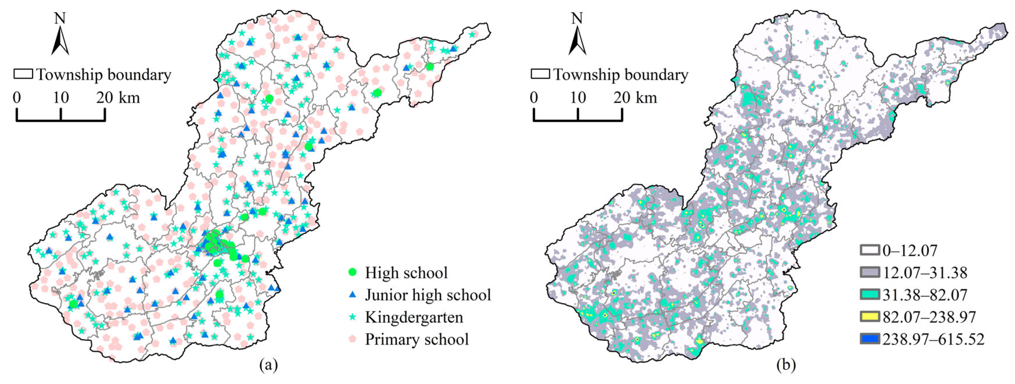
3.1.1. Spatial Density

Kernel density estimation was used to quantitatively analyze the spatial distribution density of schools in the Qixingguan District, and the natural breakpoint method was used to visualize that density; although there are common elements in the spatial distribution patterns of preschool, primary, and secondary schools in the Qixingguan District (Figure 4), there are also some key differences. School spatial density follows a pattern involving a single core with multiple centers: the central urban area is the core, and the township government stations are the centers. The performance of preschools and secondary schools is particularly obvious, whereas primary schools are spread around the township government stations. The density of preschools, primary, and secondary schools in most regions of Qixingguan District is low, although the density of schools in all three stages is high in the central urban area, which indicates that school facilities are concentrated in the central urban area.

3.1.2. Spatial Distribution of Service Capacity

The weighted summation method was used to calculate the service capacity of each school in the Qixingguan District according to the index system established in Table 1, and the inverse distance interpolation method was used for spatial visualization (Figure 5). High-level service capability for preschools is mainly distributed in the eastern region, the central city, and nearby towns, following a pattern of strength in the east-central regions and weakness in the southwest–northwest regions; for primary schools, this is concentrated in the central city, following the pattern of a dual-core with multiple centers; and for secondary schools, it is still concentrated in the central urban area, but the spatial distribution of service capacity is quite patchy. Overall, schools with a high level of service capacity are concentrated in central urban areas.

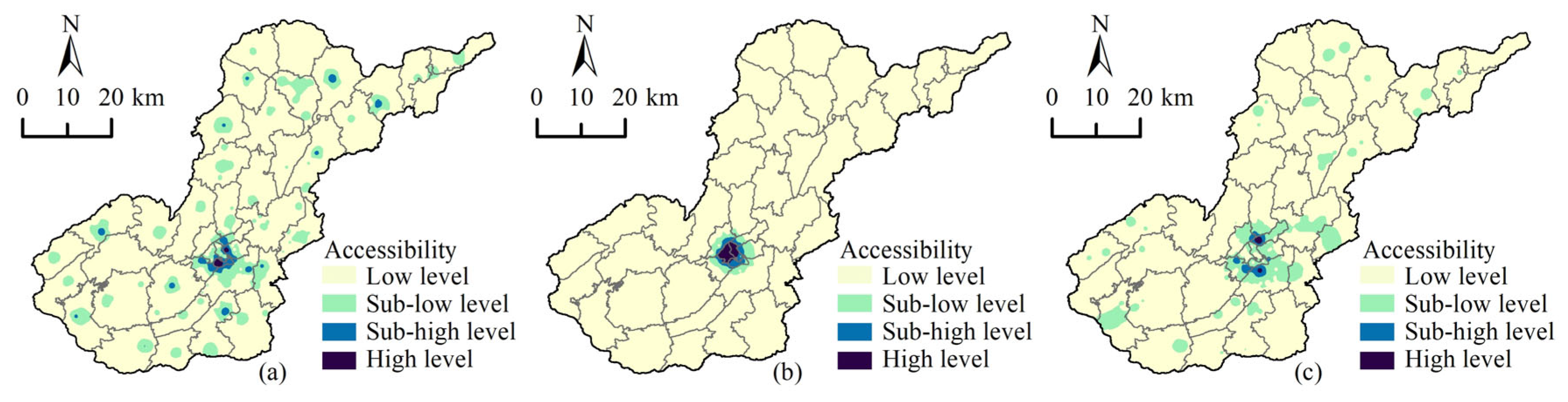
3.1.3. Spatial Accessibility

Formulas (2)–(4) were used to calculate the spatial accessibility of rural residential areas for different stages of education in Qixingguan District. The inverse distance weight interpolation method was used to visualize the accessibility. Based on the natural breakpoint method, the visualization results were divided into four levels: low, sub-low, sub-high, and high (Figure 6).

The accessibility of rural preschool education in Qixingguan District generally follows the characteristics of a single core with multiple centers. Areas with a high level of accessibility (the “single core”) are concentrated in the periphery of the central urban area, which is mainly due to the area’s large number of kindergartens, high comprehensive service capacity, and high-density road network. The “multi-center” areas with a sub-high and sub-low level of accessibility are mainly distributed in the resident centers of the township governments, which are the population-gathering units second only to the central urban areas, so there is a relatively high level of public service facilities. Areas with low accessibility are distributed in clusters in the central urban area of Qixingguan District and areas outside the town center. The small number of kindergartens and low-density road networks are the main reasons for the low accessibility.

The accessibility of rural primary schools in the Qixingguan District follows an annular distribution pattern. The high level of accessibility is concentrated in the central urban area, which has mature infrastructure construction, a concentration of the school-age population and teachers, and strong primary school accessibility. As the distance from the central urban area increases, the density of the road network gradually decreases, and accessibility is relatively weakened. The rural primary school-age population has a single travel mode, with a high travel time cost.

For secondary schools, the areas with high levels of accessibility are distributed in the central urban area with dual cores, although there are areas with a sub-high level of accessibility distributed in the periphery of areas with high accessibility, and their spatial distribution characteristics are similar. The areas with a sub-low level of accessibility are scattered in the periphery of the central urban area, the northeast and southwest regions, and low accessibility areas are distributed most widely. This indicates that the accessibility of rural secondary schools in Qixingguan District is low on the whole, and the spatial distribution is oriented toward the urban center.

3.2. School Spatial Optimization Analysis

3.2.1. Assumption of the Optimal Layout

By analyzing the spatial layout and accessibility of schools at different stages, it can be seen that the spatial pattern of school accessibility for the rural school-age population in Qixingguan District is not connected to the distribution of school density or service capacity. There are two main reasons for this phenomenon. First, the supply of schools is dislocated—that is, the schools at each stage are not in the optimal position, and the number of schools within the range of the rural school-age population’s willingness to travel is small, which increases the travel time cost. Second, there is insufficient school service capacity—that is, within the range of travel willingness for the rural school-age population, the service capacity of accessible schools is weak. Given the dislocation of the quantity and supply of schools, this study considered the limited number of schools, combined with the current situation of the transportation network in Qixingguan District, and sought to reduce the travel time for the rural school-age population and to optimize the location of schools at each stage. The service capacity of schools at each stage was also optimized, given the insufficient radiation of the school service capacity, considering the construction scale and level of the existing schools, and minimizing the spatial accessibility of schools for the rural school-age population.

3.2.2. The Effect of Location Optimization on Schools

A location optimization model was used to optimize the location of 340 preschools, 426 primary schools, and 109 secondary schools in Qixingguan District to minimize students’ travel time costs to educational facilities at different stages. Figure 7 shows that, after optimization, the center of the standard deviation ellipse for preschools and secondary schools migrated to the northeast, the area and angle of the standard deviation ellipse increase, and the proportion of the short axis to the long axis of the standard deviation ellipse decreases. After optimization, the center of the standard deviation ellipse for primary schools moved in a northeasterly direction, the angle of the standard deviation ellipse, the proportion of the short axis to the long axis of the standard deviation ellipse increased, and the area of the standard deviation ellipse decreased. The number of schools at different stages increased in the northeast of Qixingguan District, and the number of preschools and secondary schools was relatively dispersed toward the northeast. Primary schools were relatively concentrated in the northeast.

3.2.3. The Effect of Optimization on Service Capability

The service capability optimization model was applied after location optimization. The descriptive statistical differences in the service capability of schools at each stage before and after optimization are shown in Figure 8, and the differences in spatial distribution are shown in Figure 9. From a statistical perspective, the median service capacity of preschools, primary schools, and secondary schools after optimization increased, while the standard deviation, range, and coefficient of variation after optimization were all smaller than before optimization, which indicates, first, the difference between the level of the school service capacity and the average level fell after optimization and, second, after optimization, the differences in service capacity among schools also fell. From the perspective of spatial distribution, compared with before the optimization (Figure 5), Spatially, after optimization, the high-level service capability of preschools spread to the southwest and northwest, following a multiple core pattern in the southwest and northwest. For primary schools, this capacity was tightened in the central and northwest regions, showing strength in the central region and weakness in the eastern and western regions. For secondary schools, high-level capacity spread to the central part of the district, and the number of core areas increased significantly.

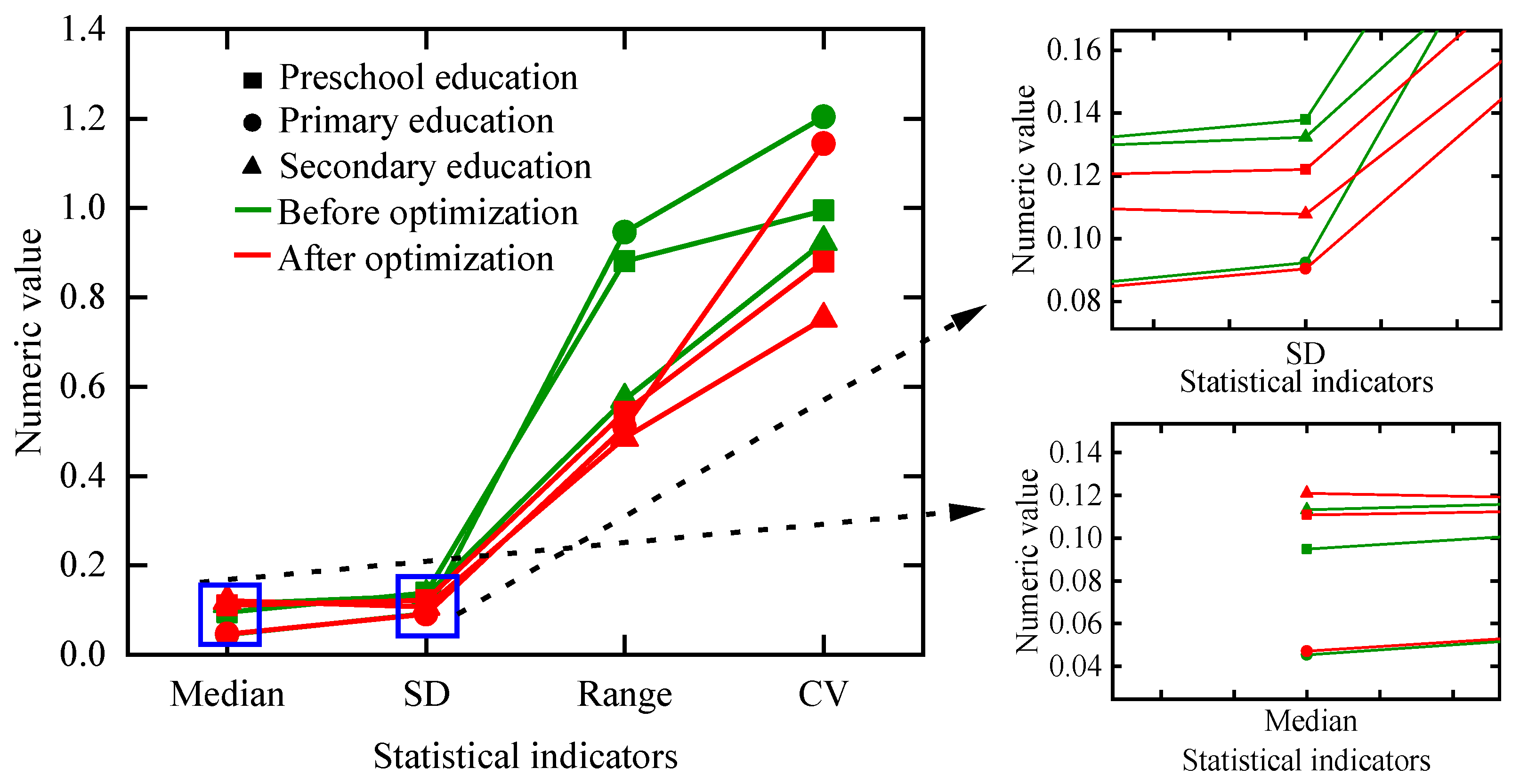
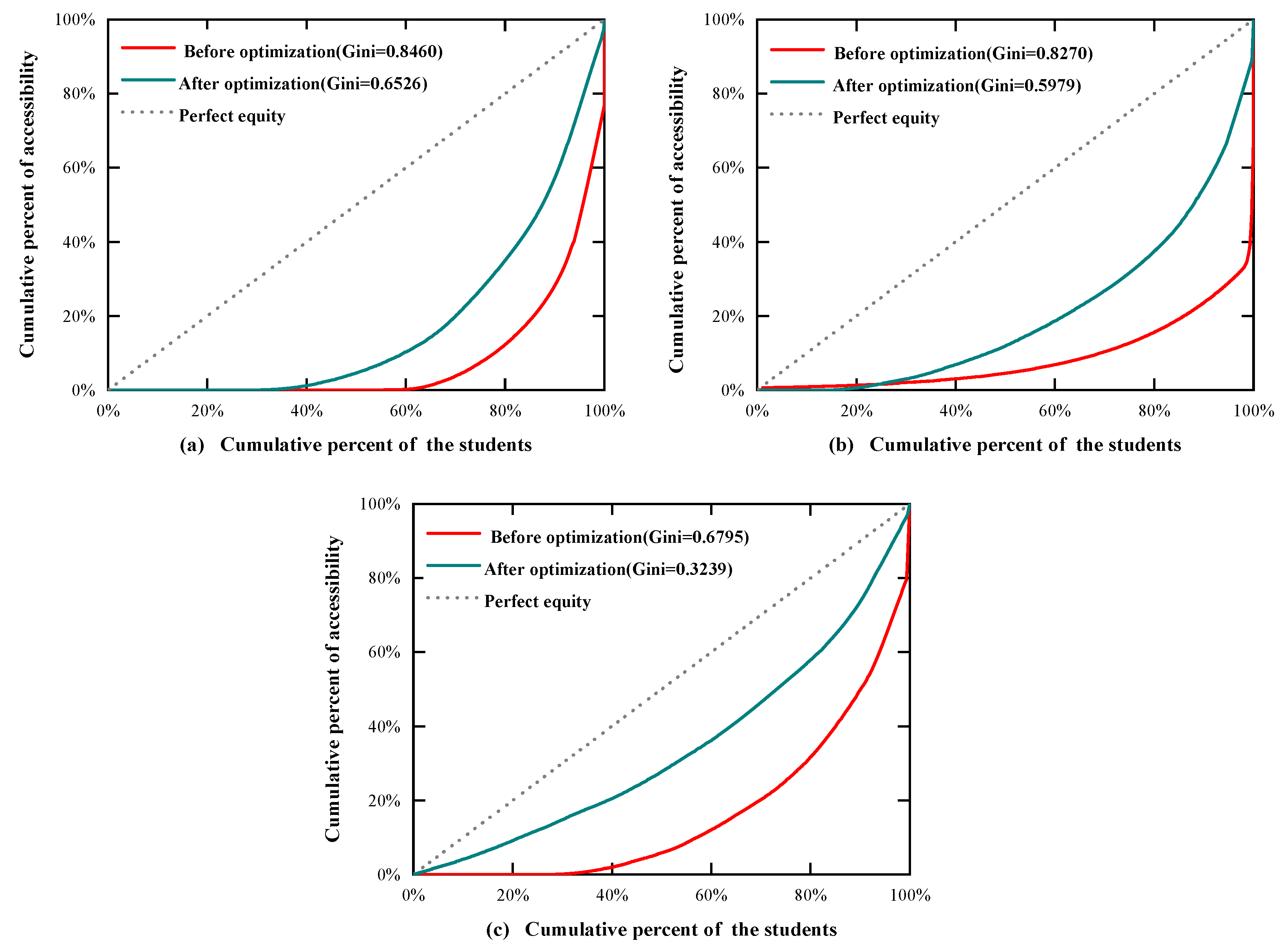
3.2.4. The Effect of Optimization on Accessibility

1. Spatial Distribution of Accessibility

Based on the natural breakpoint method, the visualization results were divided into four grades: low, sub-low, sub-high, and high; the number and proportion of rural residential areas and the school-age population in different grades were counted (Table 3 and Figure 10).

(1) Comparison of preschool accessibility

After optimization, the areas with high, sub-high, and low levels of preschool accessibility in Qixingguan District increased significantly and were mainly distributed in the southwest and northeast regions, whereas areas with a low level of accessibility decreased significantly and were concentrated in the central urban and southeast areas. Before optimization, the number of rural residential settlements and the school-age population within the low level of accessibility for rural preschools was the largest, reaching 19,839 and 254,683 people, accounting for 86.66% and 85.30% of the total, respectively; after optimization, these numbers decreased significantly, accounting for 37.88% and 38.74% of the total, while the number of rural settlements in the low level, sub-high level, and high-level accessibility areas increased significantly.

(2) Comparison of primary school accessibility

After optimization, the spatial pattern of rural primary school accessibility tended to be more balanced. There are more areas with high, sub-high, and low levels of accessibility, and they are generally distributed in the southwest and northeast of the district, while the scope of low-level accessibility areas fell significantly and was concentrated in the central urban and southeastern areas. Before optimization, the number of rural residential settlements and the school-age population with a low level of accessibility to rural primary schools was the largest, reaching 22,436 and 292,215 people, accounting for 98.00% and 97.84% of the total number of the whole district, respectively; after optimization, these numbers accounted for only about 50% of the total number of regions, whereas the number of rural residential settlements and the school-age population in the sub-low-level accessibility area increased significantly. Although the proportion of rural residential settlements and school-age populations in the sub-high and high-level accessibility areas remained small, the number of rural residential settlements and the school-age population was significantly improved compared to before optimization.

(3) Comparison of secondary school accessibility

After optimization, the areas with low, sub-high, and high levels of rural secondary school accessibility increased significantly and were concentrated in the northeast and southwest, while the areas with a low level of accessibility increased significantly, concentrated in the central urban area and the southwest. Before optimization, the number of rural residential settlements and the school-age population with a low level of accessibility to rural secondary schools was the largest, reaching 20,410 and 251,327 people, accounting for 89.15% and 84.18% of the total number for the whole district, respectively. After optimization, these numbers decreased to 56.03% and 55.19%, and the quantity of rural residential settlements and the school-age population in the low-level accessibility area increased significantly. Although the proportion of rural residential settlements and the school-age population in sub-high and high-level accessibility areas remained small, it was significantly improved compared to before optimization.

Figure 10. Spatial accessibility distribution of school after optimization: (a) Spatial accessibility of preschool; (b) Spatial accessibility of primary school; (c) Spatial accessibility of secondary school.

Figure 10. Spatial accessibility distribution of school after optimization: (a) Spatial accessibility of preschool; (b) Spatial accessibility of primary school; (c) Spatial accessibility of secondary school.

Table 3. Rural settlements and school-age populations within different accessibility levels.

Education Stage	Level of Accessibility	Before Optimization				After Optimization
		Settlement	Proportion (%)	Population	Proportion (%)	Settlement	Proportion (%)	Population	Proportion (%)
Preschool	Low level	19,839	86.66	254,683	85.30	8672	37.88	115,661	38.74
	Sub-low level	2704	11.81	38,229	12.80	7508	32.80	102,601	34.36
	Sub-high level	346	1.51	5637	1.89	5040	22.02	62,764	21.02
	High level	4	0.02	17	0.01	1673	7.31	17,540	5.87
Primary school	Low level	22,436	98.00	292,115	97.84	12,241	53.47	168,156	56.32
	Sub-low level	352	1.54	4795	1.61	8921	38.97	109,664	36.73
	Sub-high level	98	0.43	1575	0.53	1482	6.47	17,980	6.02
	High level	7	0.03	81	0.03	249	1.09	2766	0.93
Secondary school	Low level	20,410	89.15	251,327	84.18	12,827	56.03	164,776	55.19
	Sub-low level	2224	9.71	42,031	14.08	6744	29.46	90,966	30.47
	Sub-high level	215	0.94	3407	1.14	2017	8.81	25,410	8.51
	High level	44	0.19	1801	0.60	1305	5.70	17,414	5.83

Table 3. Rural settlements and school-age populations within different accessibility levels.

Education Stage	Level of Accessibility	Before Optimization				After Optimization
		Settlement	Proportion (%)	Population	Proportion (%)	Settlement	Proportion (%)	Population	Proportion (%)
Preschool	Low level	19,839	86.66	254,683	85.30	8672	37.88	115,661	38.74
	Sub-low level	2704	11.81	38,229	12.80	7508	32.80	102,601	34.36
	Sub-high level	346	1.51	5637	1.89	5040	22.02	62,764	21.02
	High level	4	0.02	17	0.01	1673	7.31	17,540	5.87
Primary school	Low level	22,436	98.00	292,115	97.84	12,241	53.47	168,156	56.32
	Sub-low level	352	1.54	4795	1.61	8921	38.97	109,664	36.73
	Sub-high level	98	0.43	1575	0.53	1482	6.47	17,980	6.02
	High level	7	0.03	81	0.03	249	1.09	2766	0.93
Secondary school	Low level	20,410	89.15	251,327	84.18	12,827	56.03	164,776	55.19
	Sub-low level	2224	9.71	42,031	14.08	6744	29.46	90,966	30.47
	Sub-high level	215	0.94	3407	1.14	2017	8.81	25,410	8.51
	High level	44	0.19	1801	0.60	1305	5.70	17,414	5.83

2. Overall Accessibility Equilibrium Analysis

This study calculates the average value of the spatial accessibility of educational facilities at all stages in Qixingguan District before and after optimization, and performs a paired sample t-test. As shown in

Table 4. Paired sample t-test results of optimization before and after accessibility mean values.

Education Stage	Before Optimization	After Optimization	T	p
Preschool education	0.0020	0.1456	−21.441	0.000
Primary education	0.0014	0.1462	−21.523	0.000
Secondary education	0.0066	0.5597	−48.560	0.000

, there is a significant difference between the paired samples before and after optimization (|t| > 1.96, p < 0.05), and the average value of spatial accessibility of educational facilities at all stages after optimization is significantly higher than that before optimization.

The Lorentz curve and Gini coefficient were used to quantitatively analyze the equilibrium of the spatial distribution of accessibility at different stages of education in rural Qixingguan District before and after optimization. Accessibility was arranged in ascending order. The cumulative percentage of the school-age population was taken as the horizontal axis and the cumulative percentage of accessibility was taken as the vertical axis to draw the Lorentz curve for the spatial distribution of school accessibility (Figure 11). The Gini coefficient was then calculated using the geometric block approximation method; it takes a value between 0 and 1: the higher the value, the more unfair the spatial distribution of accessibility. Figure 7 shows that before and after optimization, the Lorentz curves for the spatial distributions of the accessibility of preschools, primary schools, and secondary schools in Qixingguan District all deviated from the absolute mean line, but compared with before optimization, the optimized Lorentz curves all tended to be closer to that absolute mean line, and the Gini coefficients all showed a decreasing trend after optimization. This indicates that the spatial distribution of school accessibility tended to be more balanced after model optimization, and the model is thus reliable for optimizing the spatial distribution of rural educational resources in Qixingguan District.

4. Discussion

The kernel density estimation and entropy method were used to calculate the spatial distribution characteristics of the density and service capacity of multi-stage educational facilities in a mountainous area of China, and Ga2SFCA was used to quantitatively evaluate spatial accessibility characteristics. On this basis, problems in the spatial distribution of schools in a mountainous area of China were analyzed. Compared with other studies [12,50], this paper conducted field investigations on the travel modes and acceptable time of the school-age population, optimized the scale and location of educational facilities to improve the fairness of school entry opportunities for school-age population in mountainous areas, and analyzed the optimization effect, which can provide a reference for selecting the location of basic schools in mountainous areas and the allocation of education service capacity. This paper does, however, still have some shortcomings.

First, road networks are an important data basis for calculating travel costs for the school-age population. The road network data were extracted based on census data from national geographic conditions and they were identified and divided according to different administrative levels. It was assumed that the road networks identified in this way were the only roads that the school-age population could use to go to school, whereas convenient paths are common in mountainous and rural areas. However, this study could not accurately identify and incorporate such information into the road network, leading to a certain deviation in the calculation of travel costs. Additionally, in future studies, the means of data acquisition should be enriched, and dynamic factors such as population aging and birth rate should be added to the optimization model to enhance the practical significance of the research.

Second, during location optimization, alternative school locations are crucial. This study excluded the ecological red line and buildable areas of basic farmland, but did not consider the impact of terrain factors such as slope and altitude on school construction. Future studies should consider more factors that would affect the difficulty and cost of school construction to make the selection of alternative locations of schools more scientific.

Finally, the optimization of school service capacity in this paper aimed to maximize the accessibility of rural schools. However, the schools involved in this paper also provide educational services for the urban school-age population. By only considering the accessibility of rural schools, the educational service capacity of the whole region is optimized, but this will affect the equity of the education received by the urban residents in the region. In future studies, the accessibility of both urban and rural schools should be taken into account, and a more practical service capacity optimization scheme for schools should be designed.

5. Conclusions

Although there are common elements in the spatial distribution of the density and service capacity of preschools, primary schools, and secondary schools in the rural areas of Qixingguan District, there are also some key differences. Schools at all stages are concentrated in the central urban area, and the service capacity of schools in the central urban area is high. The main difference lies in variations in spatial equilibrium: preschools have the strongest equilibrium in the distribution of service capacity, followed by primary schools and then secondary schools as the weakest; while for density distribution, primary schools had the strongest equilibrium, followed by secondary schools, with preschools have the weakest equilibrium. The spatial imbalance in the capacity of educational facilities’ services and the density of facilities indicates a core challenge in Qixingguan District’s pursuit of sustainable education development—the issue of educational equity. The imbalance, particularly in primary and secondary education, highlights the lack of educational resources in terms of supply and spatial layout, urgently necessitating optimized resource allocation to achieve the goals of sustainable educational development.

Before optimization, the level of accessibility for schools in rural areas of Qixingguan District was generally poor, and the spatial patterns differed by education stage. Preschool education accessibility generally followed a single core with multiple center patterns, while primary school accessibility presented an annular distribution pattern, and secondary school accessibility had an obvious dual-core feature. The imbalance in spatial accessibility will exacerbate the inequality in the distribution of educational resources between urban and rural areas, impacting the realization of sustainable educational development. The main causes of this phenomenon were the dislocation of the quantity and supply of schools and the mismatch of service capacity. Therefore, it is essential to improve educational accessibility by focusing on both the location of educational facilities and the capacity of services, thereby providing scientific support for sustainable educational development.

The optimization results based on the location and the scale optimization model showed that, after optimization, the schools in each stage spread to the northeast; the service capacity differences between schools and between regions fell; the areas with a high, sub-high, and low level of accessibility expanded. The overall equilibrium of spatial accessibility improved, which verified the reliability of the optimization model. This optimization approach, by enhancing the efficiency of spatial allocation of educational facilities, increases the opportunities for school-age children in rural areas to access educational resources, strengthens the sustainable supply capacity of educational resources, and provides practical support for achieving the goal of sustainable educational development.

References

1. Oloko-oba, M.; Ogunyemi, A.S.; Alaga, A.T.; Olatunji, S.B.; Ibrahim, S.I.; Isa, I.; Kolawole, M.H. A geospatial approach to evaluation of accessibility to government primary schools in Ilorin west local government area, Kwara State, Nigeria. Eur. Int. J. Sci. Technol. 2015, 4, 96–107. [Google Scholar]
2. Gao, Y.; He, Q.; Liu, Y.; Zhang, L.; Wang, H.; Cai, E. Imbalance in spatial accessibility to primary and secondary schools in China: Guidance for education sustainability. Sustainability 2016, 8, 1236. [Google Scholar] [CrossRef]
3. Bali Swain, R.; Ranganathan, S. Modeling interlinkages between sustainable development goals using network analysis. World Dev. 2021, 138, 105136. [Google Scholar] [CrossRef]
4. Strulik, H. The return to education in terms of wealth and health. J. Econ. Ageing 2018, 12, 1–14. [Google Scholar] [CrossRef]
5. Yang, J.; Qiu, M. The impact of education on income inequality and intergenerational mobility. China Econ. Rev. 2016, 37, 110–125. [Google Scholar] [CrossRef]
6. Adejumo, O.O.; Asongu, S.A.; Adejumo, A.V. Education enrolment rate vs. employment rate: Implications for sustainable human capital development in Nigeria. Int. J. Educ. Dev. 2021, 83, 102385. [Google Scholar] [CrossRef]
7. Martinez, W. How science and technology developments impact employment and education. Proc. Natl. Acad. Sci. USA 2018, 115, 12624–12629. [Google Scholar] [CrossRef]
8. Bertoletti, A.; Berbegal-Mirabent, J.; Agasisti, T. Higher education systems and regional economic development in Europe: A combined approach using econometric and machine learning methods. Socio-Econ. Plan. Sci. 2022, 82, 101231. [Google Scholar] [CrossRef]
9. Unterhalter, E. The many meanings of quality education: Politics of targets and indicators in SDG4. Glob. Policy 2019, 10, 39–51. [Google Scholar] [CrossRef]
10. United Nations. Transforming Our World: The 2030 Agenda for Sustainable Development. 2015. Available online: https://sdgs.un.org/2030agenda (accessed on 1 August 2019).
11. Asadikia, A.; Rajabifard, A.; Kalantari, M. Systematic prioritisation of SDGs: Machine learning approach. World Dev. 2021, 140, 105269. [Google Scholar] [CrossRef]
12. Han, Z.; Dong, M.; Liu, T.; Li, Y. Spatial accessibility evaluation and layout optimization of basic education facilities in community life circle: A case study of Shahekou in Dalian. Sci. Geogr. Sin. 2020, 40, 1774–1783. [Google Scholar]
13. Tsou, K.; Hung, Y.; Chang, Y. An accessibility-based integrated measure of relative spatial equity in urban public facilities. Cities 2005, 22, 424–435. [Google Scholar] [CrossRef]
14. Hu, L. Racial/ethnic differences in job accessibility effects: Explaining employment and commutes in the Los Angeles region. Transp. Res. Part D Transp. Environ. 2019, 76, 56–71. [Google Scholar] [CrossRef]
15. Lu, N.; Li, J.; Yan, H.; Tuo, S.; Ying, L. Analysis on accessibility of urban park green space: The case study of Shenyang Tiexi District. J. Appl. Ecol. 2014, 25, 2951–2958. [Google Scholar]
16. Yang, L.; Wang, B.; Zhou, J.; Wang, X. Walking accessibility and property prices. Transp. Res. Part D Transp. Environ. 2018, 62, 551–562. [Google Scholar] [CrossRef]
17. Zheng, Z.; Shen, W.; Li, Y.; Qin, Y.; Wang, L. Spatial equity of park green space using KD2SFCA and web map API: A case study of zhengzhou, China. Appl. Geogr. 2020, 123, 102310. [Google Scholar] [CrossRef]
18. Cao, Y.; Guo, Y.; Zhang, M. Research on the equity of urban green park space layout based on Ga2SFCA optimization method-taking the core area of Beijing as an example. Land 2022, 11, 1323. [Google Scholar] [CrossRef]
19. Li, W.; Guan, H.; Han, Y.; Zhu, H.; Zhao, P. Accessibility of multimode transport facilities to suburban tourist attractions: Analysis based on meso-or microcommunity scale in Beijing. J. Urban Plan. Dev. 2021, 147, 4021026. [Google Scholar] [CrossRef]
20. Zhang, J.; Han, P.; Sun, Y.; Zhao, J.; Yang, L. Assessing spatial accessibility to primary health care services in Beijing, China. Int. J. Environ. Res. Public Health 2021, 18, 13182. [Google Scholar] [CrossRef]
21. Mao, K.; Chen, Y.; Wu, G.; Huang, J.; Yang, W.; Xia, Z. Measuring spatial accessibility of urban fire services using historical fire incidents in Nanjing, China. ISPRS Int. J. Geo-Inf. 2020, 9, 585. [Google Scholar] [CrossRef]
22. Dai, D.; Wang, F. Geographic disparities in accessibility to food stores in southwest Mississippi. Environ. Plan. B Plan. Des. 2011, 38, 659–677. [Google Scholar] [CrossRef]
23. Tao, Z.; Cheng, Y.; Dai, T.; Rosenberg, M. Spatial optimization of residential care facility locations in Beijing, China: Maximum equity in accessibility. Int. J. Health Geogr. 2014, 13, 33. [Google Scholar] [CrossRef] [PubMed]
24. Yang, X.; Xia, B.; Jin, M.; Wang, Z. Analysis of county and rural compulsory education accessibility and balance based on mm3sfca: A case study of Shouxian County, Anhui Province. Areal Res. Dev. 2024, 43, 166–173. [Google Scholar]
25. Luo, W.; Whippo, T. Variable catchment sizes for the two-step floating catchment area (2SFCA) method. Health Place 2012, 18, 789–795. [Google Scholar] [CrossRef]
26. McGrail, M.; Humphreys, J. Measuring spatial accessibility to primary health care services: Utilising dynamic catchment sizes. Appl. Geogr. 2014, 54, 182–188. [Google Scholar] [CrossRef]
27. Abankina, I.; Filatova, L. Accessibility of pre-school education. Vopr. Obraz./Educ. Stud. Mosc. 2018, 3, 216–246. [Google Scholar] [CrossRef]
28. Guo, N.; Wang, L.; Chang, F.; Ma, P.; Liao, T.; Fu, M. Evaluation and optimization strategy of equivalence of preschool education resources based on community life circle: A case study of the main urban area of Lanzhou City. Econ. Geogr. 2024, 44, 84–94. [Google Scholar]
29. Xu, Y.; Song, W.; Liu, C. Social-Spatial Accessibility to Urban Educational Resources under the School District System: A Case Study of Public Primary Schools in Nanjing, China. Sustainability 2018, 10, 2305. [Google Scholar] [CrossRef]
30. Zheng, L.; Xiao, T.; Liu, Y.; Qin, R.; Chai, L.; Yao, J. Using multiple travel mode two-step floating catchment area (2SFCA) approach to measure the spatial accessibility of primary schools in Dongguan City, China. Prog. Geogr. 2023, 42, 1341–1354. [Google Scholar] [CrossRef]
31. Williams, S.; Wang, F. Disparities in accessibility of public high schools, in metropolitan Baton Rouge, Louisiana 1990–2010. Urban Geogr. 2014, 35, 1066–1083. [Google Scholar] [CrossRef]
32. Wu, Y.; Zheng, X.; Sheng, L.; You, H. Exploring the equity and spatial evidence of educational facilities in Hangzhou, China. Soc. Indic. Res. 2020, 151, 1075–1096. [Google Scholar] [CrossRef]
33. Lin, J.; Huang, Y.; He, J. School accessibility and academic achievement in a rural area of Taiwan. Child. Geogr. 2014, 12, 232–248. [Google Scholar] [CrossRef]
34. Wen, H.; Zhang, Y.; Zhang, L. Do educational facilities affect housing price? An empirical study in Hangzhou, China. Habitat Int. 2014, 42, 155–163. [Google Scholar] [CrossRef]
35. Wen, H.; Xiao, Y.; Hui, E.; Zhang, L. Education quality, accessibility, and housing price: Does spatial heterogeneity exist in education capitalization? Habitat Int. 2018, 78, 68–82. [Google Scholar] [CrossRef]
36. Wang, X.; Hu, J.; Qiu, B. The impact of public service facilities on housing prices from the perspective of spatiotemporal accessibility: A study based on multiscale geographically weighted regression model (MGWR). Mod. Urban Res. 2024, 38, 116–122. [Google Scholar]
37. Liao, C.; Scheuer, B.; Dai, T.; Tian, Y. Optimizing the spatial assignment of schools to reduce both inequality of educational opportunity and potential opposition rate through introducing random mechanism into proximity-based system. Socio-Econ. Plan. Sci. 2020, 72, 100893. [Google Scholar] [CrossRef]
38. Dai, T.; Liao, C.; Zhao, S. Optimizing the spatial assignment of schools through a random mechanism towards equal educational opportunity: A resemblance approach. Comput. Environ. Urban Syst. 2019, 76, 24–30. [Google Scholar] [CrossRef]
39. Delmelle, E.; Thill, J.; Peeters, D.; Thomas, I. A multi-period capacitated school location problem with modular equipment and closest assignment considerations. J. Geogr. Syst. 2014, 16, 263–286. [Google Scholar] [CrossRef]
40. Bouzarth, E.; Forrester, R.; Hutson, K.; Reddoch, L. Assigning students to schools to minimize both transportation costs and socioeconomic variation between schools. Socio-Econ. Plan. Sci. 2018, 64, 1–8. [Google Scholar] [CrossRef]
41. Li, X.; Wang, F.; Yi, H. A two-step approach to planning new facilities towards equal accessibility. Environ. Plan. B Urban Anal. City Sci. 2017, 44, 994–1011. [Google Scholar] [CrossRef]
42. Han, Z.; Du, P.; Wang, L.; Yu, Y.; Zhao, D.; Cong, Y.; Ren, Q. Method for optimization allocation of regional public service infrastructure: A case study of Xinghua Street primary school. Sci. Geogr. Sin. 2014, 34, 803–809. [Google Scholar]
43. Lotfi, R.; Pilehforooshha, P.; Karimi, M. A multi-objective optimization model for school location-allocation coupling demographic changes. J. Spat. Sci. 2021, 68, 225–244. [Google Scholar] [CrossRef]
44. Cai, A.; Tao, Z.; Wang, J.; Li, G. Accessibility assessment and spatial optimization of educational facilities in newly urbanized areas: A case of Pingshan District, Shenzhen City. Areal Res. Dev. 2021, 40, 96–102. [Google Scholar]
45. Zhang, Y.; Sun, J.; Du, L.; Zhou, L. Analyzing spatial accessibility to secondary education resources in Liupanshui area. Sci. Surv. Mapp. 2019, 44, 52–58. [Google Scholar]
46. JTGB01-2014; Technical Standard of Highway Engineering. Ministry of Transport of the People’s Republic of China: Beijing, China, 2014.
47. Chen, J.; Wang, C.; Zhang, Y.; Li, D. Measuring spatial accessibility and supply-demand deviation of urban green space: A mobile phone signaling data perspective. Front. Public Health 2022, 10, 1029551. [Google Scholar] [CrossRef]
48. Lu, Y.; Fang, S. Study on the spatial distribution optimization of park green spaces in the main city of Wuhan from the perspective of both equilibrium and efficiency. Resour. Environ. Yangtze Basin 2019, 28, 68–79. [Google Scholar]
49. Wang, F.; Tang, Q. Planning toward equal accessibility to services: A quadratic programming approach. Environ. Plan. B Plan. Des. 2013, 40, 195–212. [Google Scholar] [CrossRef]
50. Chen, W.; Yang, L.; Sun, J.; Pan, B. Research on rural primary school layout optimization based on spatial equity: A case study on Huangping County in Guizhou Province. Areal Res. Dev. 2021, 40, 138–142. [Google Scholar]
Figure 1. Schematic diagram of Qixingguan District and its road network.
Sustainability 17 03862 g001
Figure 2. Spatial distribution of schools and school-age population in Qixingguan District: (a) Spatial distribution of school; (b) Spatial distribution of school-age population.
Sustainability 17 03862 g002
Figure 3. Technical routes for educational equity and optimization.
Sustainability 17 03862 g003
Figure 4. Spatial distribution of school density before optimization: (a) Density of preschool; (b) Density of primary school; (c) Density of secondary school.
Sustainability 17 03862 g004
Figure 5. Spatial distribution of school service capacity before optimization: (a) Service capacity of preschool; (b) Service capacity of primary school; (c) Service capacity of secondary school.
Sustainability 17 03862 g005
Figure 6. Spatial accessibility of school before optimization: (a) Accessibility of preschool; (b) Accessibility of primary school; (c) Accessibility of secondary school.
Sustainability 17 03862 g006
Figure 7. School locations and standard deviation ellipse distribution before and after optimization: (a) Locations and standard deviation ellipse of preschool; (b) Locations and standard deviation ellipse of primary school; (c) Locations and standard deviation ellipse of secondary school.
Sustainability 17 03862 g007
Figure 8. Descriptive statistics for school service capacity before and after optimization.
Sustainability 17 03862 g008
Figure 9. Spatial distribution of school service capacity after optimization: (a) Service capacity of preschool; (b) Service capacity of primary school; (c) Service capacity of secondary school.
Sustainability 17 03862 g009
Figure 11. Lorentz curve of the spatial distribution of accessibility before and after optimization: (a) Lorentz curve of preschool; (b) Lorentz curve of primary school; (c) Lorentz curve of secondary school.
Sustainability 17 03862 g011