


Evaluation and Prediction of Ecological Quality Based on Remote Sensing Environmental Index and Cellular Automata-Markov

 , , , and
Abstract
1. Introduction
- (i)
- A comprehensive method for assessing and predicting ecological environment quality is proposed, which integrates the RSEI with the CA-Markov model. By leveraging the spatial characteristics of remote sensing data and the dynamic spatiotemporal simulation capabilities of the CA-Markov model, this approach achieved integrated ecological environment analysis in the Johor region, addressing the research gap in large-scale, long-term time series prediction of ecological environment dynamics.
- (ii)
- Quantitative spatial distribution and temporal trend analysis reveal long-term ecological change patterns and the relationship between regional differences in ecological quality and spatial aggregation characteristics, providing a theoretical foundation for formulating ecological conservation and restoration strategies.
- (iii)
- Spatial autocorrelation analysis is introduced to identify spatiotemporal distribution patterns of priority ecological conservation zones, vulnerable areas, and transitional regions through autocorrelation analysis of ecological quality data across different periods. This significantly enhances the understanding of spatial heterogeneity in regional ecological environments.
- (iv)
- Based on spatiotemporal analysis results, this study proposed targeted ecological protection and management strategies for rapidly urbanizing and industrializing zones in Johor, along with concrete recommendations for balancing economic development and ecological conservation. The policy implications offer valuable references for ecological environment management in similar regions.
2. Materials and Methods
2.1. Materials
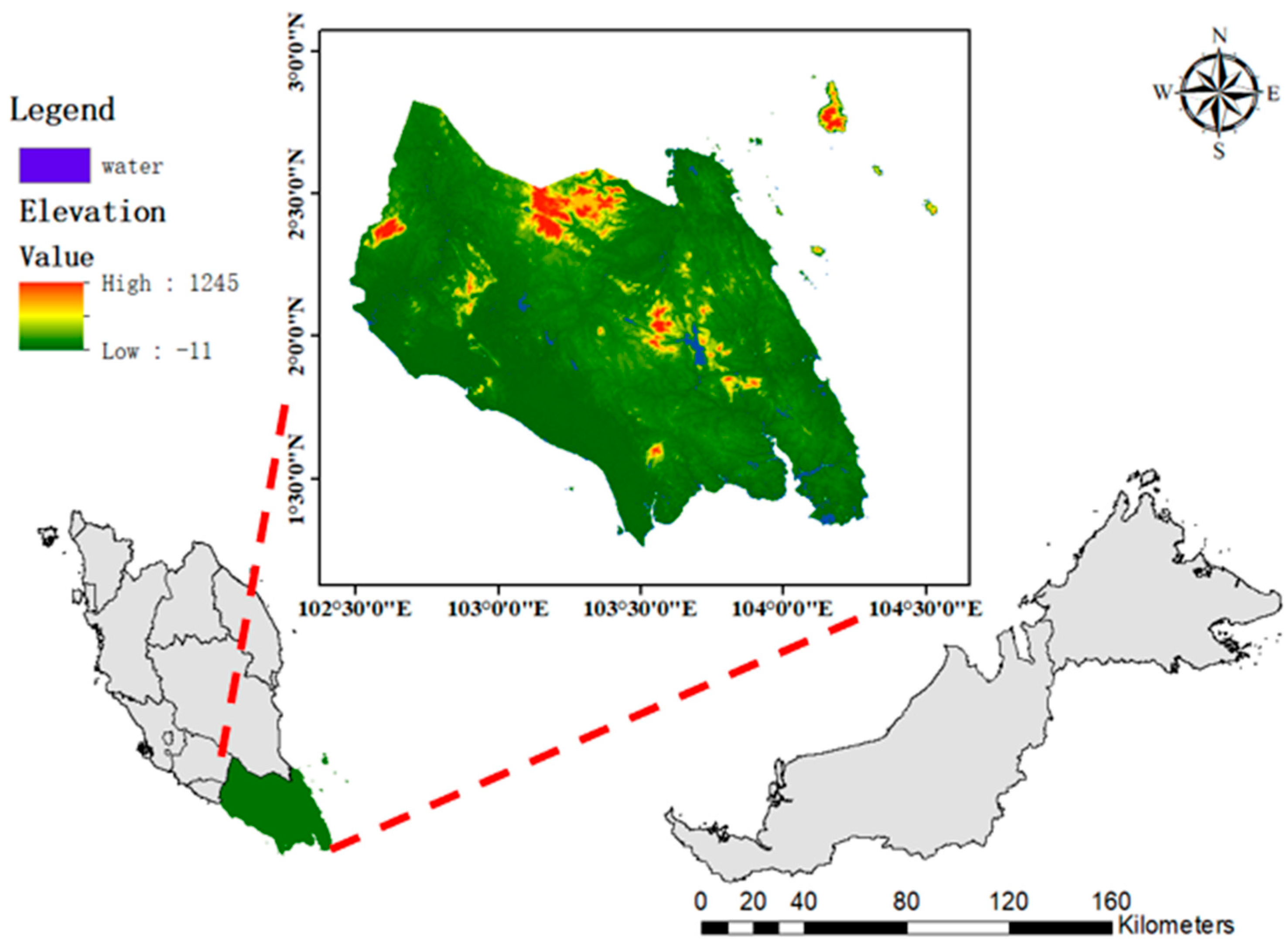
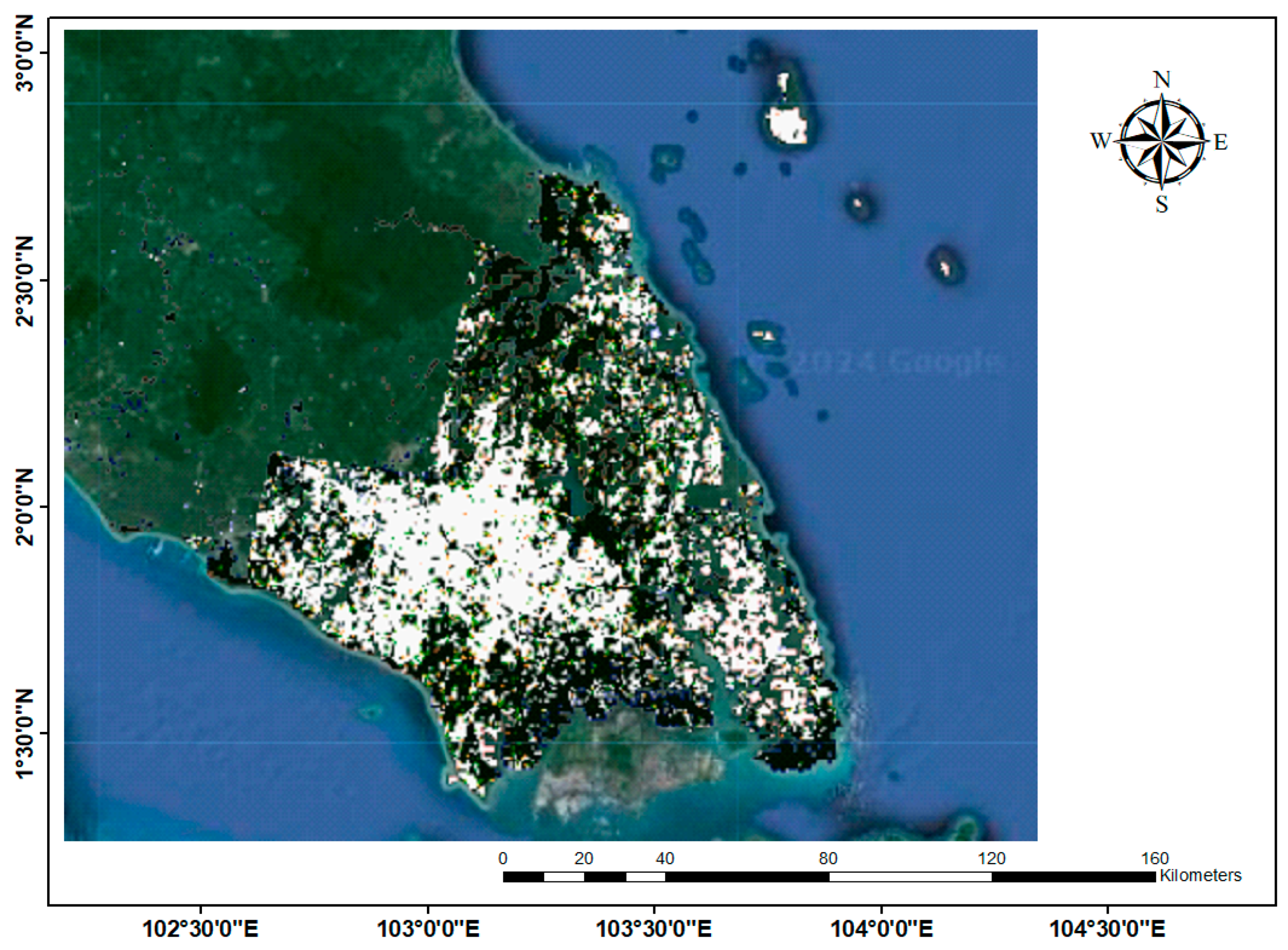
2.1.1. Study Area
2.1.2. Data Sources
2.2. Methods
2.2.1. Remote Sensing Ecological Index (RSEI)
2.2.2. Spatial Auto-Correlation Analysis
2.2.3. Cellular Automata-Markov (CA-Markov)
2.2.4. Rolling Forecast Validation
3. Results and Analysis
3.1. Factor Attributes
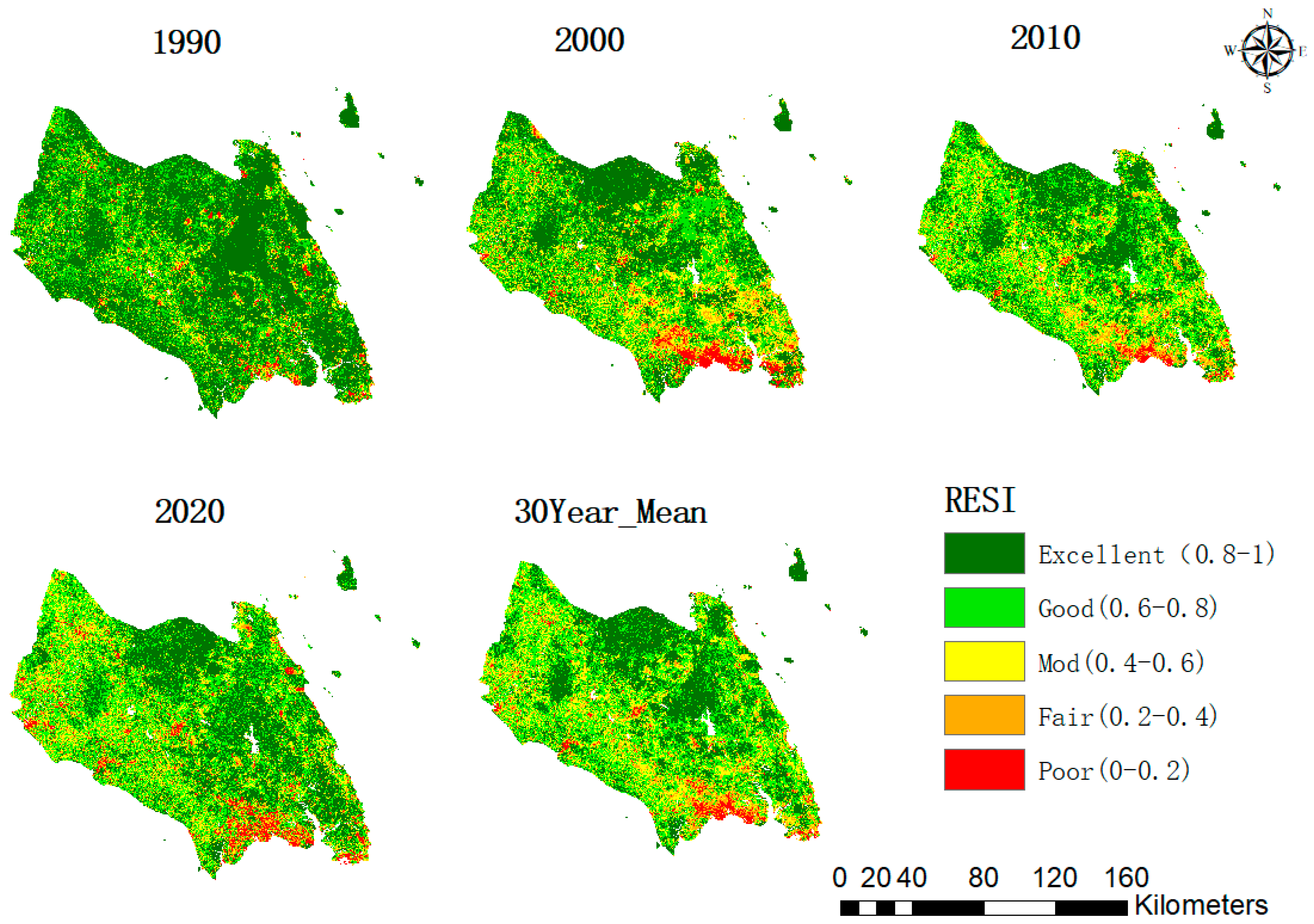
3.2. Spatiotemporal Distribution and Changes in Ecological Environmental Quality
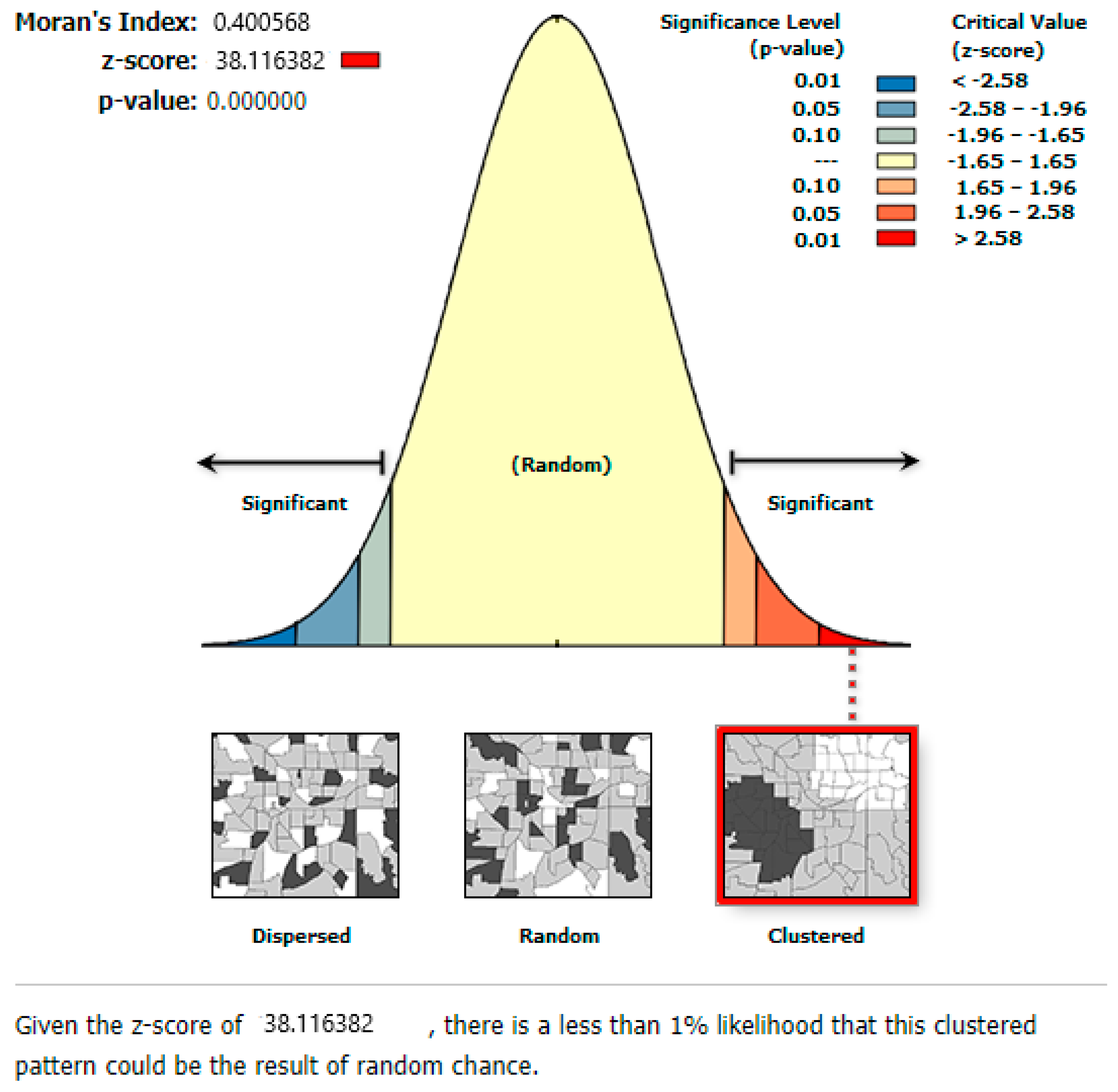
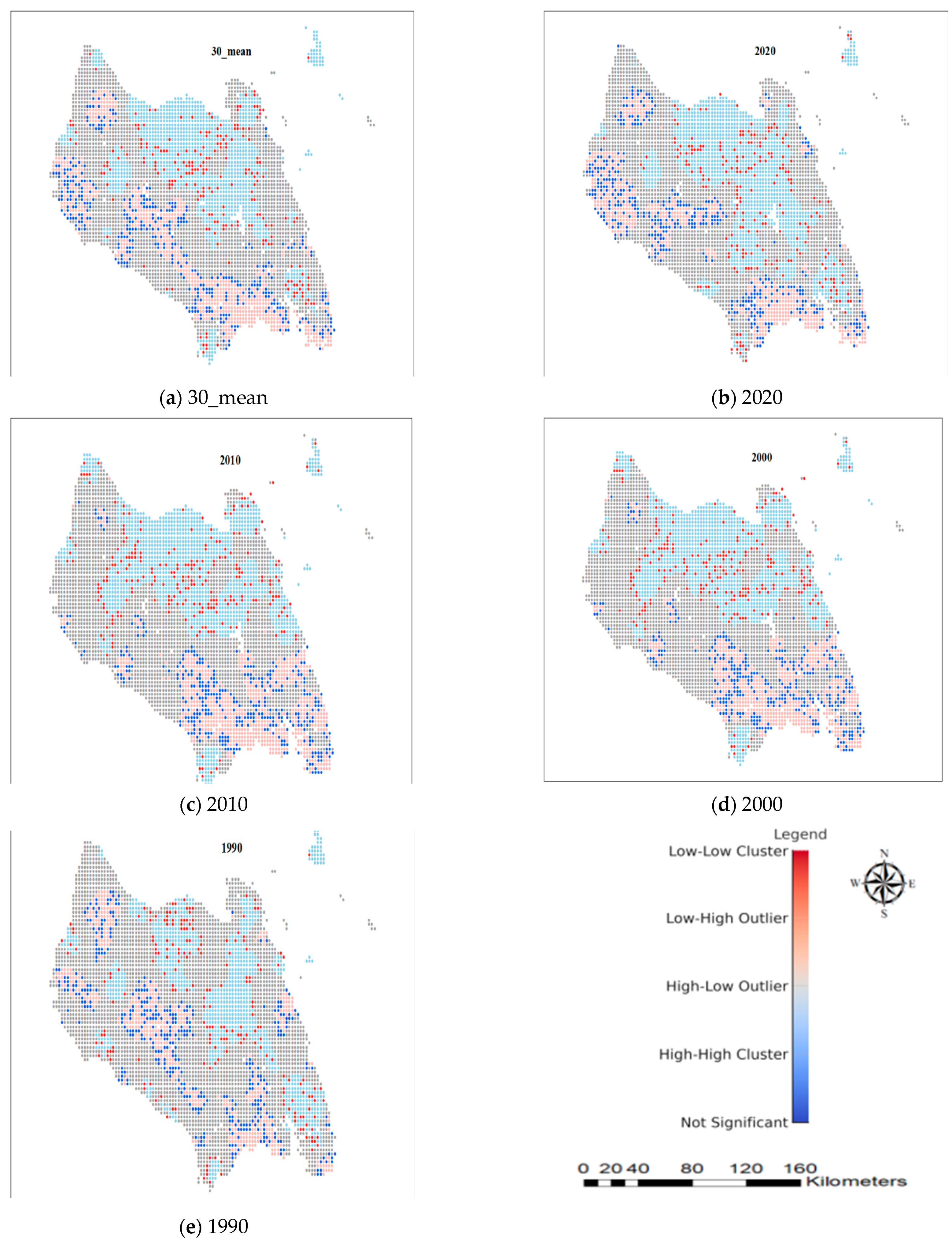
3.3. Spatial Autocorrelation Analysis of Ecological Quality
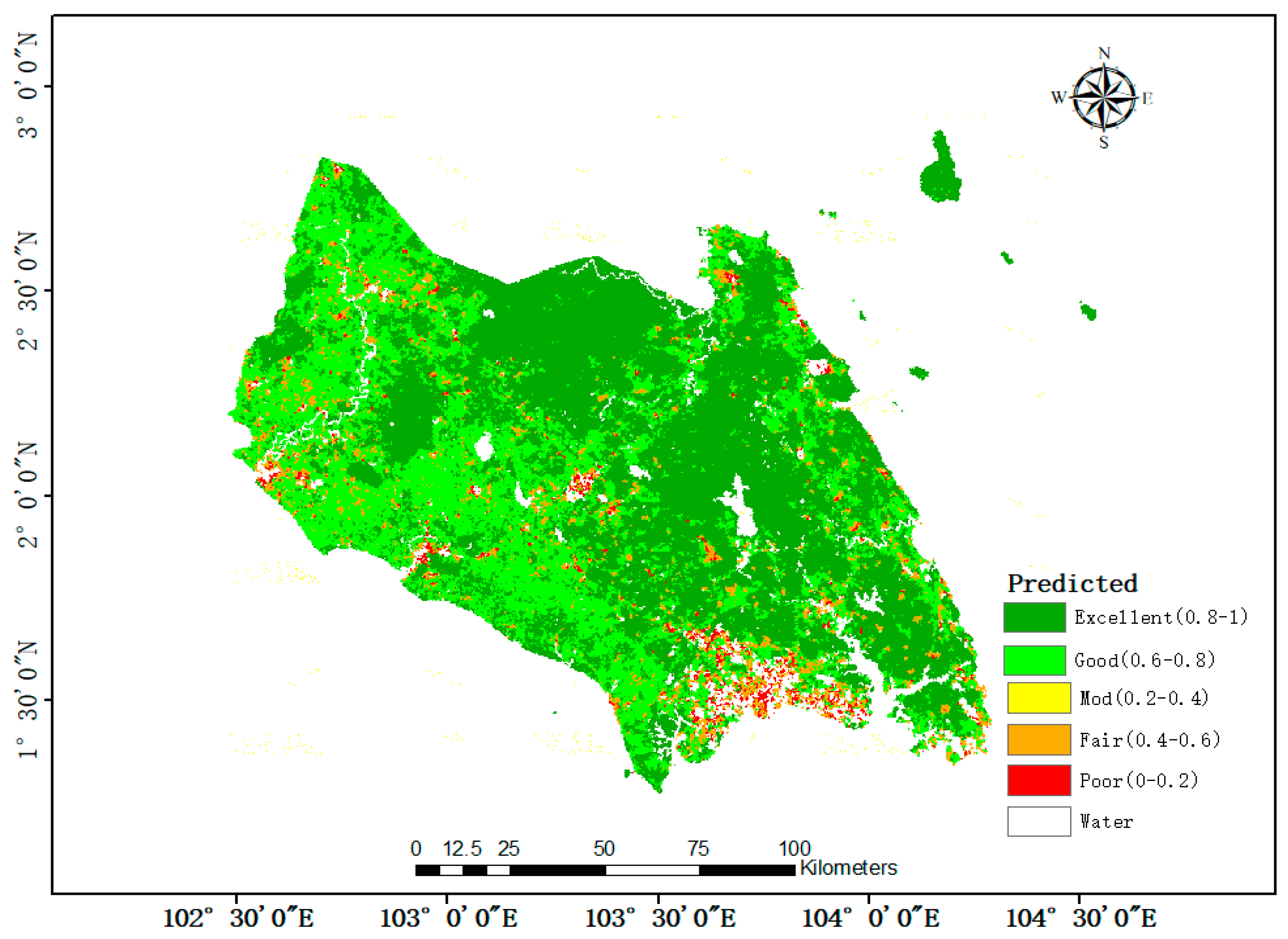
3.4. One-Year Distribution of RSEI for Johor Area
4. Discussion
5. Conclusions
Author Contributions
Funding
Institutional Review Board Statement
Informed Consent Statement
Data Availability Statement
Acknowledgments
Conflicts of Interest
Abbreviations
| RSEI | Remote Sensing Environmental Index |
| CA-Markov | Cellular Automata-Markov |
| NDVI | Normalized Difference Vegetation Index |
| EVI | Enhanced Vegetation Index |
| PCA | principal component analysis |
| MSRE | Multi-Indicator Remote Sensing Ecological Index |
| IRSEI | Integrated Remote Sensing Ecological Index |
| WET | Wetness Index |
| NDBSI | Normalized Difference Built-up Space Index |
| LST | and Land Surface Temperature |
References
- Helali, J.; Asaadi, S.; Jafarie, T.; Habibi, M.; Salimi, S.; Momenpour, S.E.; Shahmoradi, S.; Hosseini, S.A.; Hessari, B.; Saeidi, V. Drought monitoring and its effects on vegetation and water extent change using remote sensing data in Urmia Lake watershed, Iran. J. Water Clim. Change 2022, 13, 2107–2128. [Google Scholar] [CrossRef]
- Zheng, Z.; Wu, Z.; Chen, Y.; Yang, Z.; Marinello, F. Exploration of eco-environment and urbanization changes in coastal zones: A case study in China over the past 20 years. Ecol. Indic. 2020, 119, 106847. [Google Scholar] [CrossRef]
- Huete, A.; Didan, K.; Miura, T.; Rodriguez, E.P.; Gao, X.; Ferreira, L.G. Overview of the radiometric and biophysical performance of the MODIS vegetation indices. Remote Sens. Environ. 2002, 83, 195–213. [Google Scholar] [CrossRef]
- Lu, D.; Mausel, P.; Brondízio, E.; Moran, E. Change detection techniques. Int. J. Remote Sens. 2004, 25, 2365–2401. [Google Scholar] [CrossRef]
- Running, S.W.; Zhao, M. User’s Guide for MODIS Land Products (Collection 6): MOD17A2/A3—MODIS GPP and NPP. NASA. 2015. Available online: https://modis.gsfc.nasa.gov/data/dataprod/mod17.php (accessed on 9 April 2014).
- Wan, Z. MODIS Land Surface Temperature Products Users’ Guide; Institute for Computational Earth System Science, University of California: Santa Barbara, CA, USA, 2006; p. 805. [Google Scholar]
- Dekker, A.G.; Peters, S.W.M. The use of the Thematic Mapper for the analysis of eutrophic lakes: A case study in The Netherlands. Int. J. Remote Sens. 1993, 14, 799–821. [Google Scholar] [CrossRef]
- Turner, W.; Spector, S.; Gardiner, N.; Fladeland, M.; Sterling, E.; Steininger, M. Remote sensing for biodiversity science and conservation. Trends Ecol. Evol. 2003, 18, 306–314. [Google Scholar] [CrossRef]
- Ozesmi, S.L.; Bauer, M.E. Satellite remote sensing of wetlands. Wetl. Ecol. Manag. 2002, 10, 381–402. [Google Scholar] [CrossRef]
- Parmesan, C.; Yohe, G. A globally coherent fingerprint of climate change impacts across natural systems. Nature 2003, 421, 37–42. [Google Scholar] [CrossRef] [PubMed]
- Xu, H.Q. A remote sensing urban ecological index and its application. Acta Ecol. Sin. 2013, 33, 7853–7862. [Google Scholar] [CrossRef]
- Hang, X.; Li, Y.; Luo, X.; Xu, M.; Han, X. Assessing the ecological quality of Nanjing during its urbanization process by using satellite, meteorological, and socioeconomic data. J. Meteorol. Res. 2020, 34, 280–293. [Google Scholar] [CrossRef]
- Li, P. Research on ecoenvironmental quality evaluation system based on big data analysis. Comput. Intell. Neurosci. 2022, 2022, 5191223. [Google Scholar] [CrossRef] [PubMed]
- Shan, W.; Jin, X.; Ren, J.; Wang, Y.; Xu, Z.; Fan, Y.; Gu, Z.; Hong, C.; Lin, J.; Zhou, Y. Ecological environment quality assessment based on remote sensing data for land consolidation. J. Clean. Prod. 2019, 239, 118126. [Google Scholar] [CrossRef]
- Xu, H.; Wang, M.; Shi, T.; Guan, H.; Fang, C.; Lin, Z. Prediction of ecological effects of potential population and impervious surface increases using a remote sensing based ecological index (RSEI). Ecol. Indic. 2018, 93, 730–740. [Google Scholar] [CrossRef]
- Jiang, C.L.; Wu, L.; Liu, D.; Wang, S.M. Dynamic monitoring of eco-environmental quality in arid desert area by remote sensing: Taking the Gurbantunggut Desert China as an example. Ying Yong Sheng Tai Xue Bao J. Appl. Ecol. 2019, 30, 877–883. [Google Scholar]
- Li, S.; Li, X.; Gong, J.; Dang, D.; Dou, H.; Lyu, X. Quantitative analysis of natural and anthropogenic factors influencing vegetation NDVI changes in temperate drylands from a spatial stratified heterogeneity perspective: A case study of Inner Mongolia Grasslands, China. Remote Sens. 2022, 14, 3320. [Google Scholar] [CrossRef]
- Wang, J.; Wang, J.; Xu, J. Spatio-temporal variation and prediction of ecological quality based on remote sensing ecological index–a case study of Zhanjiang City, China. Front. Ecol. Evol. 2023, 11, 1153342. [Google Scholar] [CrossRef]
- Cheng, L.L.; Wang, Z.W.; Tian, S.F.; Liu, Y.T.; Sun, M.Y.; Yang, Y.M. Evaluation of eco-environmental quality in Mentougou District of Beijing based on improved remote sensing ecological index. Chin. J. Ecol. 2021, 40, 1177. [Google Scholar]
- Akbari, M.; Shalamzari, M.J.; Memarian, H.; Gholami, A. Monitoring desertification processes using ecological indicators and providing management programs in arid regions of Iran. Ecol. Indic. 2020, 111, 106011. [Google Scholar] [CrossRef]
- Kosmas, C.; Kairis, O.; Karavitis, C.; Ritsema, C.; Salvati, L.; Acikalin, S.; Alcalá, M.; Alfama, P.; Atlhopheng, J.; Barrera, J.; et al. Evaluation and selection of indicators for land degradation and desertification monitoring: Methodological approach. Environ. Manag. 2014, 54, 951–970. [Google Scholar] [CrossRef]
- Wu, S.; Gao, X.; Lei, J.; Zhou, N.; Guo, Z.; Shang, B. Ecological environment quality evaluation of the Sahel region in Africa based on remote sensing ecological index. J. Arid. Land 2022, 14, 14–33. [Google Scholar] [CrossRef]
- Wang, Y. Evaluation of lake wetland ecotourism resources based on remote sensing ecological index. Arab. J. Geosci. 2021, 14, 559. [Google Scholar] [CrossRef]
- Tang, H.; Fang, J.; Xie, R.; Ji, X.; Li, D.; Yuan, J. Impact of land cover change on a typical mining region and its ecological environment quality evaluation using remote sensing based ecological index (RSEI). Sustainability 2022, 14, 12694. [Google Scholar] [CrossRef]
- Geng, J.; Yu, K.; Xie, Z.; Zhao, G.; Ai, J.; Yang, L.; Yang, H.; Liu, J. Analysis of spatiotemporal variation and drivers of ecological quality in Fuzhou based on RSEI. Remote Sens. 2022, 14, 4900. [Google Scholar] [CrossRef]
- Xiong, Y.; Xu, W.; Lu, N.; Huang, S.; Wu, C.; Wang, L.; Dai, F.; Kou, W. Assessment of spatial–temporal changes of ecological environment quality based on RSEI and GEE: A case study in Erhai Lake Basin, Yunnan province, China. Ecol. Indic. 2021, 125, 107518. [Google Scholar] [CrossRef]
- Shan, Y.; Dai, X.; Li, W.; Yang, Z.; Wang, Y.; Qu, G.; Liu, W.; Ren, J.; Li, C.; Liang, S.; et al. Detecting spatial-temporal changes of urban environment quality by remote sensing-based ecological indices: A case study in Panzhihua city, Sichuan Province, China. Remote Sens. 2022, 14, 4137. [Google Scholar] [CrossRef]
- Yi, S.; Zhou, Y.; Zhang, J.; Li, Q.; Liu, Y.; Guo, Y.; Chen, Y. Spatial-temporal evolution and motivation of ecological vulnerability based on RSEI and GEE in the Jianghan Plain from 2000 to 2020. Front. Environ. Sci. 2023, 11, 1191532. [Google Scholar] [CrossRef]
- Zhang, F.; Wang, Y.; Jim, C.Y.; Chan, N.W.; Tan, M.L.; Kung, H.T.; Shi, J.; Li, X.; He, X. Analysis of Urban Expansion and Human–Land Coordination of Oasis Town Groups in the Core Area of Silk Road Economic Belt, China. Land 2023, 12, 224. [Google Scholar] [CrossRef]
- Zhang, Y.; She, J.; Long, X.; Zhang, M. Spatio-temporal evolution and driving factors of eco-environmental quality based on RSEI in Chang-Zhu-Tan metropolitan circle, central China. Ecol. Indic. 2022, 144, 109436. [Google Scholar] [CrossRef]
- Yao, K.; Halike, A.; Chen, L.; Wei, Q. Spatiotemporal changes of eco-environmental quality based on remote sensing-based ecological index in the Hotan Oasis, Xinjiang. J. Arid. Land 2022, 14, 262–283. [Google Scholar] [CrossRef]
- Luo, M.; Zhang, S.; Huang, L.; Liu, Z.; Yang, L.; Li, R.; Lin, X. Temporal and spatial changes of ecological environment quality based on RSEI: A case study in Ulan Mulun river basin, China. Sustainability 2022, 14, 13232. [Google Scholar] [CrossRef]
- Gao, P.; Kasimu, A.; Zhao, Y.; Lin, B.; Chai, J.; Ruzi, T.; Zhao, H. Evaluation of the temporal and spatial changes of ecological quality in the Hami oasis based on RSEI. Sustainability 2020, 12, 7716. [Google Scholar] [CrossRef]
- Karbalaei Saleh, S.; Amoushahi, S.; Gholipour, M. Spatiotemporal ecological quality assessment of metropolitan cities: A case study of central Iran. Environ. Monit. Assess. 2021, 193, 305. [Google Scholar] [CrossRef]
- Xia, Q.Q.; Chen, Y.N.; Zhang, X.Q.; Ding, J.L. Spatiotemporal changes in ecological quality and its associated driving factors in Central Asia. Remote Sens. 2022, 14, 3500. [Google Scholar] [CrossRef]
- Li, Y.; Li, Y.; Yang, X.; Feng, X.; Lv, S. Evaluation and driving force analysis of ecological quality in Central Yunnan Urban Agglomeration. Ecol. Indic. 2024, 158, 111598. [Google Scholar] [CrossRef]
- Yang, X.; Bai, Y.; Che, L.; Qiao, F.; Xie, L. Incorporating ecological constraints into urban growth boundaries: A case study of ecologically fragile areas in the Upper Yellow River. Ecol. Indic. 2021, 124, 107436. [Google Scholar] [CrossRef]
- Yang, H.; Xu, W.; Yu, J.; Xie, X.; Xie, Z.; Lei, X.; Wu, Z.; Ding, Z. Exploring the impact of changing landscape patterns on ecological quality in different cities: A comparative study among three megacities in eastern and western China. Ecol. Inform. 2023, 77, 102255. [Google Scholar] [CrossRef]
- Zhou, S.; Li, W.; Zhang, W.; Wang, Z. The Assessment of the Spatiotemporal Characteristics of the Eco-Environmental Quality in the Chishui River Basin from 2000 to 2020. Sustainability 2023, 15, 3695. [Google Scholar] [CrossRef]
- Zhang, N.; Xiong, K.; Zhang, J.; Xiao, H. Evaluation and prediction of ecological environment of karst world heritage sites based on google earth engine: A case study of Libo–Huanjiang karst. Environ. Res. Lett. 2023, 18, 034033. [Google Scholar] [CrossRef]
- Wang, S.; Ge, Y. Ecological quality response to multi-scenario land-use changes in the Heihe River Basin. Sustainability 2022, 14, 2716. [Google Scholar] [CrossRef]
- Crist, E.P. A TM tasseled cap equivalent transformation for reflectance factor data. Remote Sens. Environ. 1985, 17, 301–306. [Google Scholar] [CrossRef]
- Chen, C.; Chen, H.; Liang, J.; Huang, W.; Xu, W.; Li, B.; Wang, J. Extraction of water body information from remote sensing imagery while considering greenness and wetness based on Tasseled Cap transformation. Remote Sens. 2022, 14, 3001. [Google Scholar] [CrossRef]
- Baig, M.H.A.; Zhang, L.; Shuai, T.; Tong, Q. Derivation of a tasselled cap transformation based on Landsat 8 at-satellite reflectance. Remote Sens. Lett. 2014, 5, 423–431. [Google Scholar] [CrossRef]
- Hu, X.; Xu, H. A new remote sensing index for assessing the spatial heterogeneity in urban ecological quality: A case from Fuzhou City, China. Ecol. Indic. 2018, 89, 11–21. [Google Scholar] [CrossRef]
- Jiménez-Muñoz, J.C.; Sobrino, J.A.; Skoković, D.; Mattar, C.; Cristóbal, J. Land surface temperature retrieval methods from Landsat-8 thermal infrared sensor data. IEEE Geosci. Remote Sens. Lett. 2014, 11, 1840–1843. [Google Scholar] [CrossRef]
- Fan, G.Y.; Cowley, J.M. Auto-correlation analysis of high-resolution electron micrographs of near-amorphous thin films. Ultramicroscopy 1985, 17, 345–355. [Google Scholar] [CrossRef]
- Martin, D. An assessment of surface and zonal models of population. Int. J. Geogr. Inf. Syst. 1996, 10, 973–989. [Google Scholar] [CrossRef]
- Griffith, D.A. Spatial Autocorrelation: A Primer Association of American Geographers; Resource Publications in Geography: Washington, DC, USA, 1987. [Google Scholar]
- Anselin, L. Local indicators of spatial association—LISA. Geogr. Anal. 1995, 27, 93–115. [Google Scholar] [CrossRef]
- Jing, Y.; Zhang, F.; He, Y.; Johnson, V.C.; Arikena, M. Assessment of spatial and temporal variation of ecological environment quality in Ebinur Lake Wetland National Nature Reserve, Xinjiang, China. Ecol. Indic. 2020, 110, 105874. [Google Scholar] [CrossRef]
- Hamad, R.; Balzter, H.; Kolo, K. Predicting land use/land cover changes using a CA-Markov model under two different scenarios. Sustainability 2018, 10, 3421. [Google Scholar] [CrossRef]
- Chotchaiwong, P.; Wijitkosum, S. Predicting urban expansion and urban land use changes in Nakhon Ratchasima City using a CA-Markov model under two different scenarios. Land 2019, 8, 140. [Google Scholar] [CrossRef]
- Ruben, G.B.; Zhang, K.; Dong, Z.; Xia, J. Analysis and projection of land-use/land-cover dynamics through scenario-based simulations using the CA-Markov model: A case study in guanting reservoir basin, China. Sustainability 2020, 12, 3747. [Google Scholar] [CrossRef]
- Li, L.; Noorian, F.; Moss, D.J.; Leong, P.H. Rolling window time series prediction using MapReduce. In Proceedings of the 2014 IEEE 15th International Conference on Information Reuse and Integration (IEEE IRI 2014), Redwood City, CA, USA, 13–15 August 2014; pp. 757–764. [Google Scholar]
- Inoue, A.; Jin, L.; Rossi, B. Rolling window selection for out-of-sample forecasting with time-varying parameters. J. Econom. 2017, 196, 55–67. [Google Scholar] [CrossRef]


| Data | Time | ee.ImageCollection | Resolution (m) |
|---|---|---|---|
| Landsat 5 | 1990–2012 | (“LANDSAT/LT05/C02/T1_L2”) | 30 |
| Landsat 8 | 2013–2023 | (“LANDSAT/LC08/C02/T2_L2”) | 30 |
| MODIS | (“MODIS/061/MOD11A1”) | LST_1000 | |
| Water(mask) | JRC/GSW1_3/Yearly History | 30 |
| Index | Sources | No. | |||||
|---|---|---|---|---|---|---|---|
| Xu et al., 2013 [11]; Crist, 1985 [42]; Chen et al., 2022 [43]. | (1) | ||||||
| L5_Wet = 0.0315 ∗ B1 + 0.2021 ∗ B2 + 0.3012 ∗ B3 + 0.1594 ∗ B4 − 0.6806 ∗ B5 − 0.6109 ∗ B7 | Xu et al., 2013 [11]; Crist, 1985 [42]; Baig et al., 2014 [44] | (2) | |||||
| L8_Wet = 0.1509 ∗ B2 + 0.1973 ∗ B3 + 0.3279 ∗ B4 + 0.3406 ∗ B5 − 0.7122 ∗ B6 − 0.4572 ∗ B7 | |||||||
| Xu et al., 2013 [11]; Hu et al., 2018 [45]; Jiménez-Muñoz et al., 2014 [46] | (3) | ||||||
| Xu et al., 2013 [11]; Hu et al., 2018 [45]; | (4) | ||||||
| ε = 0.004 ∗ pv + 0.986 | |||||||
| ρ = 1.438 ∗ 10−2 | DN | λ | gain | bias | K1 | K2 | |
| Landsat5 | BSWIR1=B6 | 11.450 µm | 0.0552 | 1.2378 | 607.76 | 1260.56 | |
| Landsat8 | BSWIR1=B10 | 10.895 µm | - | - | 774.89 | 1321.08 | |
| (5) | |||||||
| β1, β2, β3, and β4 are the main components of PCA | |||||||
| (6) | |||||||
| Year | Principal Component | NDVI | WET | NDBSI | LST | Percent Correlation Eigenvalue (%) | Eigenvalue |
|---|---|---|---|---|---|---|---|
| β1 | β2 | β3 | β4 | ||||
| 1990 | PC1 | 0.171 | 0.249 | −0.033 | −0.952 | 80.01 | 0.0064 |
| PC2 | 0.372 | 0.301 | −0.859 | −0.175 | 12.49 | 0.0049 | |
| PC3 | 0.329 | −0.081 | −0.467 | −0.247 | 7.35 | 0.0018 | |
| PC4 | 0.850 | 0.485 | −0.202 | 0.017 | 0.15 | 0.0011 | |
| 2000 | PC1 | 0.818 | −0.074 | −0.425 | 0.088 | 81.55 | 0.033 |
| PC2 | 0.669 | 0.030 | −0.713 | −0.203 | 10.23 | 0.004 | |
| PC3 | 0.702 | 0.213 | −0.530 | −0.423 | 7.81 | 0.003 | |
| PC4 | 0.147 | −0.097 | −0.171 | 0.032 | 0.41 | 0.001 | |
| 2010 | PC1 | 0.103 | 0.450 | −0.319 | −0.930 | 81.25 | 0.033 |
| PC2 | 0.708 | −0.361 | −0.361 | −0.180 | 9.61 | 0.004 | |
| PC3 | 0.678 | −0.129 | −0.649 | −0.317 | 8.64 | 0.003 | |
| PC4 | 0.168 | −0.091 | −0.374 | −0.036 | 0.50 | 0.001 | |
| 2020 | PC1 | 0.136 | 0.343 | −0.076 | −0.925 | 84.17 | 0.026 |
| PC2 | 0.683 | −0.696 | −0.141 | −0.169 | 10.89 | 0.003 | |
| PC3 | 0.705 | −0.624 | −0.061 | −0.331 | 4.57 | 0.001 | |
| PC4 | 0.131 | 0.088 | −0.985 | 0.068 | 0.37 | 0.001 |
| Year | 1990 | 2000 | 2010 | 2020 | ||||
|---|---|---|---|---|---|---|---|---|
| RESI Level | Area (km2) | Pct. (%) | Area (km2) | Pct. (%) | Area (km2) | Pct. (%) | Area (km2) | Pct. (%) |
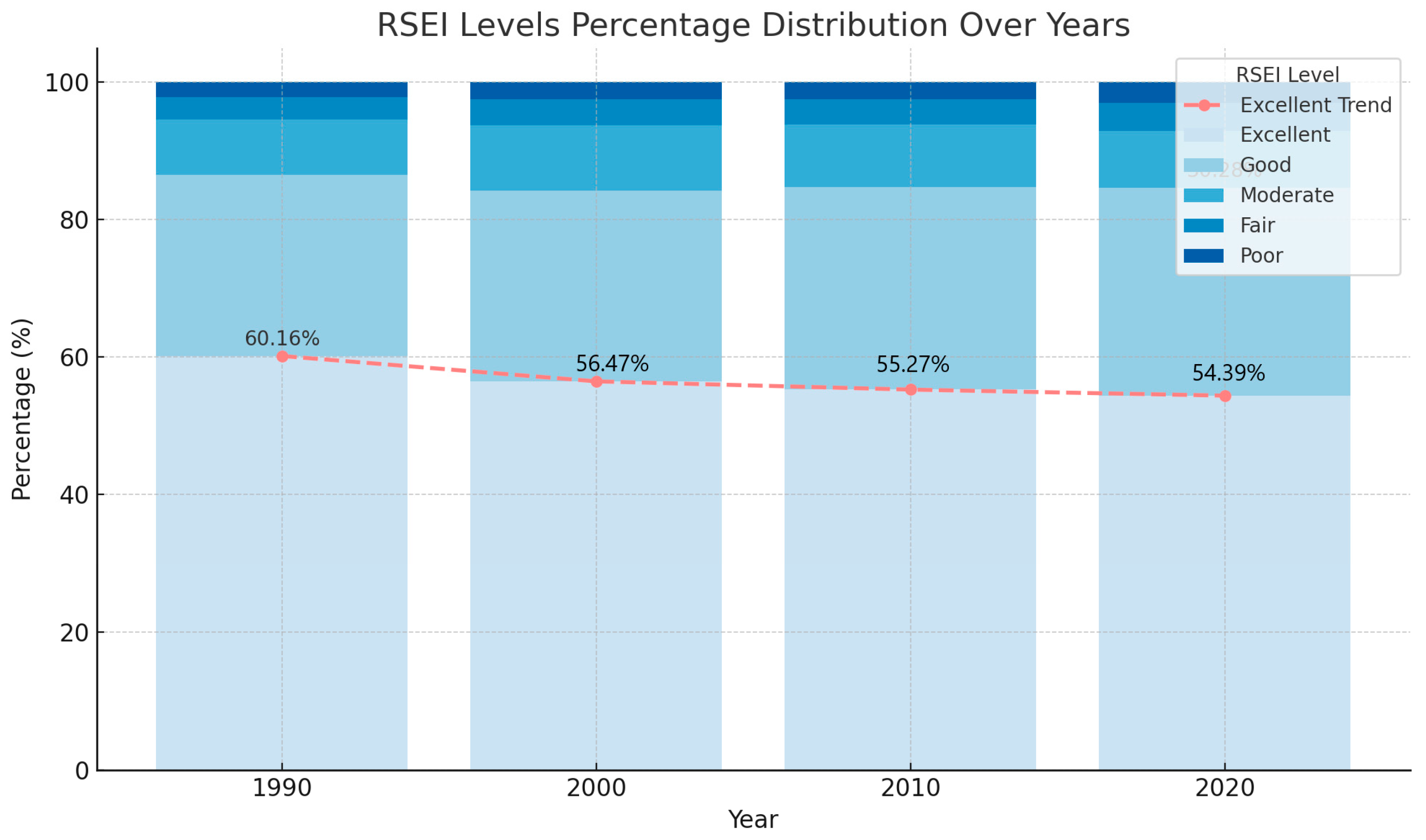
| Excellent (0.8–1) | 11,476 | 60.16 | 10,772 | 56.47 | 10543 | 55.27 | 10,376 | 54.39 |
| Good (0.6–0.8) | 5024 | 26.34 | 5288 | 27.72 | 5627 | 29.50 | 5776 | 30.28 |
| Mod (0.4–0.6) | 1552 | 8.14 | 1820 | 9.54 | 1736 | 9.10 | 1580 | 8.28 |
| Fair (0.2–0.4) | 612 | 3.21 | 704 | 3.69 | 721 | 3.78 | 731 | 3.84 |
| Poor (0–0.2) | 412 | 2.16 | 492 | 2.58 | 449 | 2.35 | 613 | 3.21 |
| 19,076 | 100.00 | 19,076 | 100.00 | 19,076 | 100.00 | 19,076 | 100.00 | |
| Interval of Years | 10 | 5 | 1 | 0 |
|---|---|---|---|---|
| No. of years | 4 | 7 | 16 | 30 |
| MSE | 0.4939 | 0.2433 | 0.1638 | 0.0778 |
| R2 | 0.9686 | 0.8219 | 0.8792 | 0.8823 |
Disclaimer/Publisher’s Note: The statements, opinions and data contained in all publications are solely those of the individual author(s) and contributor(s) and not of MDPI and/or the editor(s). MDPI and/or the editor(s) disclaim responsibility for any injury to people or property resulting from any ideas, methods, instructions or products referred to in the content. |
© 2025 by the authors. Licensee MDPI, Basel, Switzerland. This article is an open access article distributed under the terms and conditions of the Creative Commons Attribution (CC BY) license (https://creativecommons.org/licenses/by/4.0/).
Share and Cite
Qin, W.; Ismail, M.H.; Ramli, M.F.; Deng, J.; Wu, N. Evaluation and Prediction of Ecological Quality Based on Remote Sensing Environmental Index and Cellular Automata-Markov. Sustainability 2025, 17, 3640. https://doi.org/10.3390/su17083640
Qin W, Ismail MH, Ramli MF, Deng J, Wu N. Evaluation and Prediction of Ecological Quality Based on Remote Sensing Environmental Index and Cellular Automata-Markov. Sustainability. 2025; 17(8):3640. https://doi.org/10.3390/su17083640
Chicago/Turabian StyleQin, Weirong, Mohd Hasmadi Ismail, Mohammad Firuz Ramli, Junlin Deng, and Ning Wu. 2025. "Evaluation and Prediction of Ecological Quality Based on Remote Sensing Environmental Index and Cellular Automata-Markov" Sustainability 17, no. 8: 3640. https://doi.org/10.3390/su17083640
APA StyleQin, W., Ismail, M. H., Ramli, M. F., Deng, J., & Wu, N. (2025). Evaluation and Prediction of Ecological Quality Based on Remote Sensing Environmental Index and Cellular Automata-Markov. Sustainability, 17(8), 3640. https://doi.org/10.3390/su17083640