
Machine Learning in Mode Choice Prediction as Part of MPOs’ Regional Travel Demand Models: Is It Time for Change?

 ,
,
Abstract
1. Introduction
2. Literature Review
2.1. Mode Choices Within Research Body

| Study | Method | Five Built Environment Ds | ||||
|---|---|---|---|---|---|---|
| Density | Diversity | Design | Destination Accessibility | Distance to Transit | ||
| Non-motorized mode choice | ||||||
| Kockelman (1997) [21] | Logistic regression | - | Land use mix (+) | - | Job accessibility by walking (+) | - |
| Cervero & Kockelman (1997) [19] | Logistic regression | - | - | Sidewalk width (+), Proportion front and side parking (+) | - | - |
| Zhang (2004) [8] | Multinomial logit regression, Nested logit regression | Population density (+), Job density (+) | Entropy of land use balance (+) | Street connectivity (+) | - | - |
| Bento et al. (2005) [22] | Multinomial logit regression | Population density (−) | Job-housing balance (−) | - | - | Supply of rail transit (+) |
| Walk or Bike Mode Choice | ||||||
| Reilly & Landis (2002) [23] | Multinomial logit regression | Population Density (+) | Distance to closest commercial use (−) | - | - | - |
| Rajamani et al. (2003) [30] | Multinomial logit regression | - | Land use mix (+) | % Cul-de-sac street (−) | - | - |
| Ewing et al. (2004) [31] | Multinomial logit regression | - | - | Average sidewalk coverage (+) | Walk time to school (−) | - |
| Ewing et al. (2004) [31] | Multinomial logit regression | - | - | - | Bike time to school (−) | - |
| Kim et al. (2007) [24] | Multinomial logit regression | - | - | Park and ride lot at the station (−) | - | Distance between home and station (−) |
| Frank et al. (2008) [32] | Nested logit regression | Retail floor area ratio (+) | Land use mix (+) | Intersection Density (+) | - | - |
| Mitra (2012) [28] | Binomial regression | - | Jobs-to-population ratio (−) | block density (+) | - | - |
| Ozbil & Peponis (2012) [29] | Linear regression | - | Mixed-use entropy (+) | Street connectivity (+) | - | - |
| Hamre & Buehler (2014) [25] | Multinomial logit regression | Population density (+) | - | - | - | - |
| Hamre & Buehler (2014) [25] | Multinomial logit regression | Population density (+) | Urban core (+) | Bikeway supply (+) | - | - |
| Khan et al. (2014) [12] | Multinomial logit regression | - | - | 3-way intersection density (+), 4-way intersection density (+) | - | - |
| Khan et al. (2014) [12] | Multinomial logit regression | Population + Job density (−) | - | 4-way intersection density (+) | ||
| Ferrell et al. (2015) [26] | Multinomial logit regression | Population density (+) | Mixed-use (+) | 4-way intersection density (+) | - | - |
| Aziz et al. (2018) [33] | Multinomial logit regression | - | - | Sidewalk width (+) | - | - |
| Aziz et al. (2018) [33] | Mixed Logit regression | - | - | Bike land length (+), Fraction open space (+) | - | - |
| Aziz et al. (2018) [33] | Mixed Logit regression | Fraction of industrial land use (−) Fraction of residential land use in destination (−) | Sidewalk width (+) Bike lane length (+) Bike lane proportion (+) | |||
| Ton et al. (2019) [36] | Multinomial logit regression | Activity spaces (+) Presence of public buildings and shops (+) | Street furniture: garbage bins (+) playgrounds (−) Bicycle parking (+) | Suburban areas (−) | ||
| Cheng et al. (2019) [34] | Random forest | Land Entropy (+) | Road density (+) | Travel time (−) | Distance to the nearest Metro station (−) Distance to the nearest bus stop (−) Bus network density (+) Number of bus stops in 500 m neighborhood (+) | |
| Liu et al. (2021) [35] | Extreme Gradient Boosting | Population density (+) | Land use entropy (+) Job density (+) | Intersection density (+) | Trip distance (−) Distance to city center (−) | Bus stop density (+) |
2.2. Mode Choices Within Travel Demand Practices
2.2.1. Limitations of the Four-Step Models
2.2.2. Current Trends in Mode Choice Modeling Within MPO Travel Demand Practices
3. Materials and Methods
3.1. Data
3.1.1. Household Travel Survey
3.1.2. Built Environment
3.2. Variables
3.2.1. Outcome Variable
3.2.2. Explanatory Variables
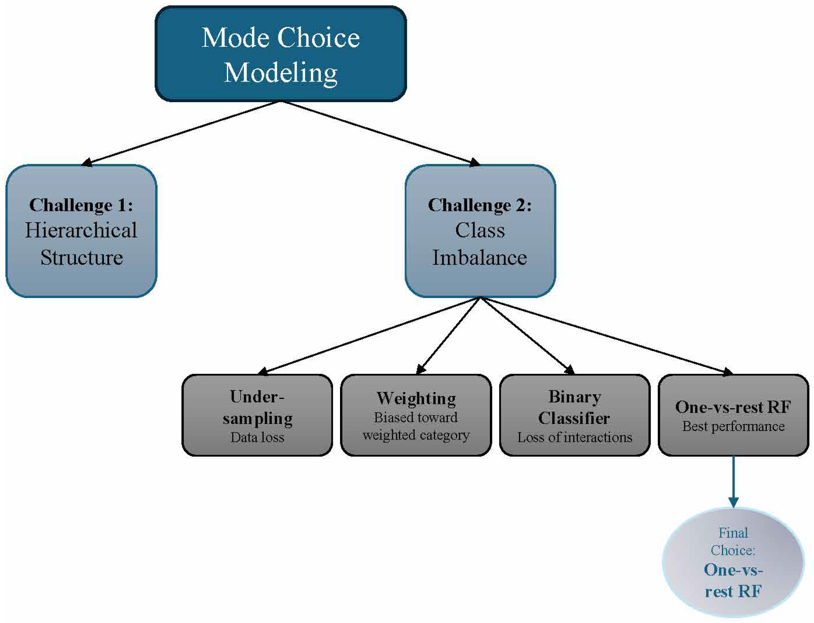
3.3. Analysis Methodology
- Under-sampling: This approach entails a random reduction in instances in the majority class (in this instance, “car”) to achieve a balanced class distribution. Employing under-sampling led to a reduction in our data size, resulting in a substantial decrease in computational time. However, it raised concerns about potential data loss.
- Weighting: We assigned varying weights to each class based on their representation in the dataset. This approach aims to provide more emphasis on the minority classes during model training to address the class imbalance issue. However, this approach presented several drawbacks. Firstly, the random forest model, when using class weights, tends to prioritize the class with higher weights, potentially leading to a biased model. Secondly, in our case, the high class imbalance resulted in an overly dominant influence of the “car” class, diminishing the model’s ability to effectively capture patterns in the minority classes. Additionally, the weighting method did not sufficiently alleviate the risk of overfitting to the majority class.
- Binary Classifier: We developed two dedicated random forest models. The first model focused exclusively on non-car trips, including “walk”, “bike”, and “transit”. The second model served as a binary classifier, distinguishing between “car” (assigned a label of 1) and “non-car” (assigned a label of 0) trips. Despite its conceptual simplicity, this approach faced challenges. Firstly, by separating the problem into two models, we lost the holistic view of interactions among all travel modes. This lack of holistic modeling could lead to information loss and suboptimal predictive performance. Additionally, predicting “non-car” as a single class might oversimplify the nuanced differences between “walk”, “bike”, and “transit”.
- One-vs-rest RF: The one-vs-rest RF method, also known as one-vs-all or unary coding, involves training a separate random forest model for each class, treating it as the positive class while grouping all other classes as the negative class. This way, we transform the multi-class classification problem into multiple binary classification problems. During prediction, the class associated with the model that yields the highest probability is assigned to the observation. This method effectively addresses class imbalance concerns and allows the random forest algorithm to provide robust predictions for each travel mode while yielding the best performance measures.
4. Results and Discussion
4.1. Performance Measures
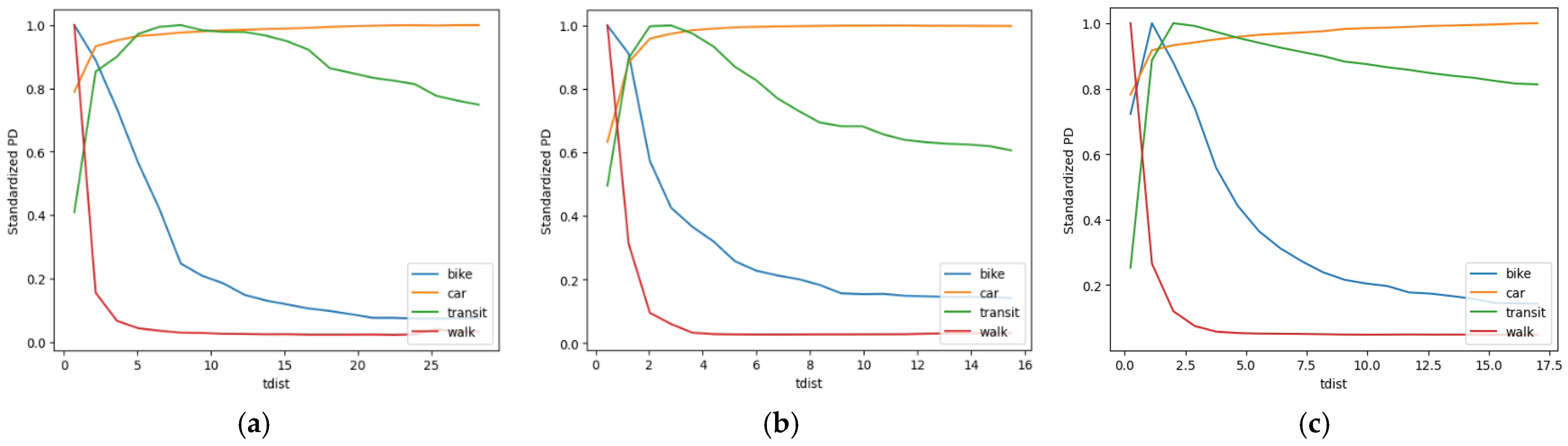
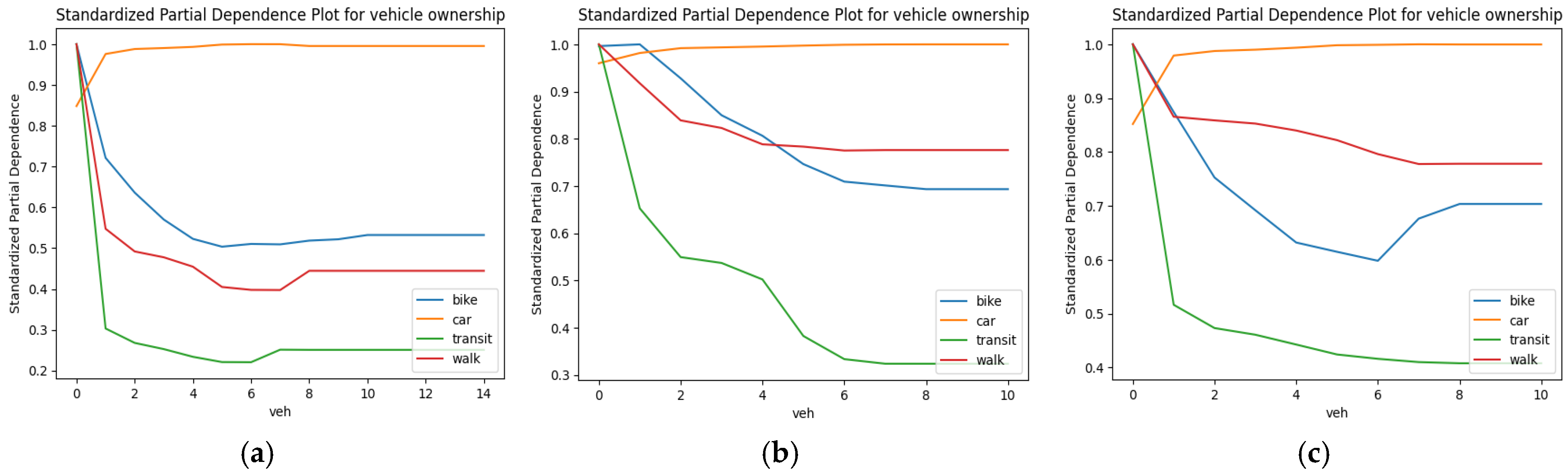
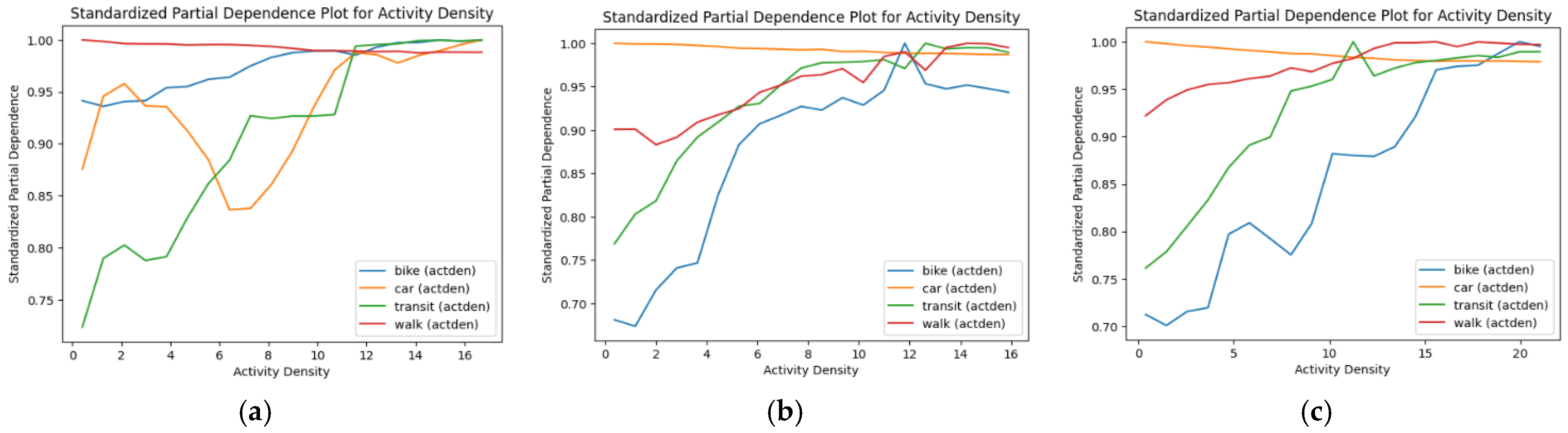
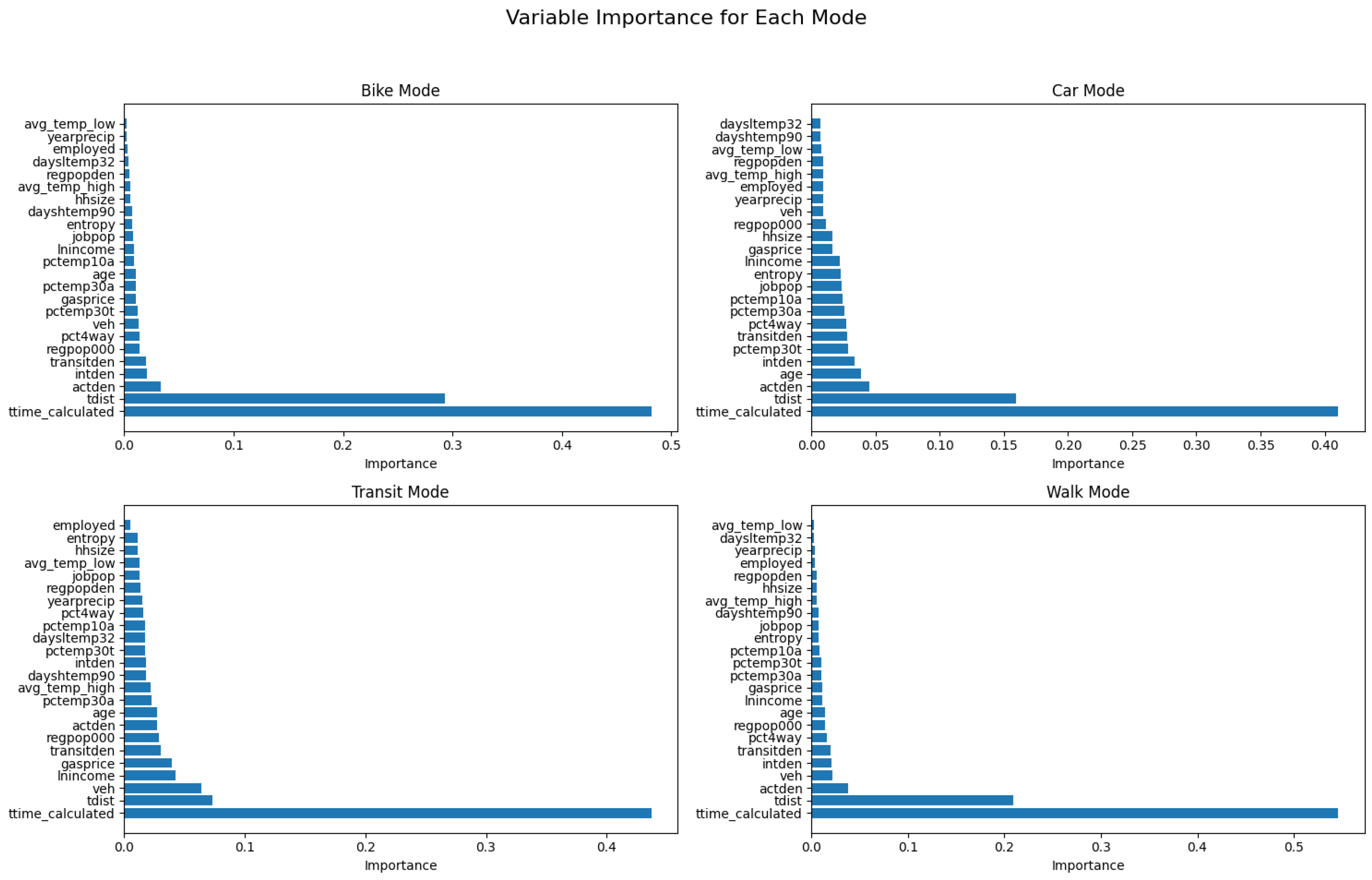
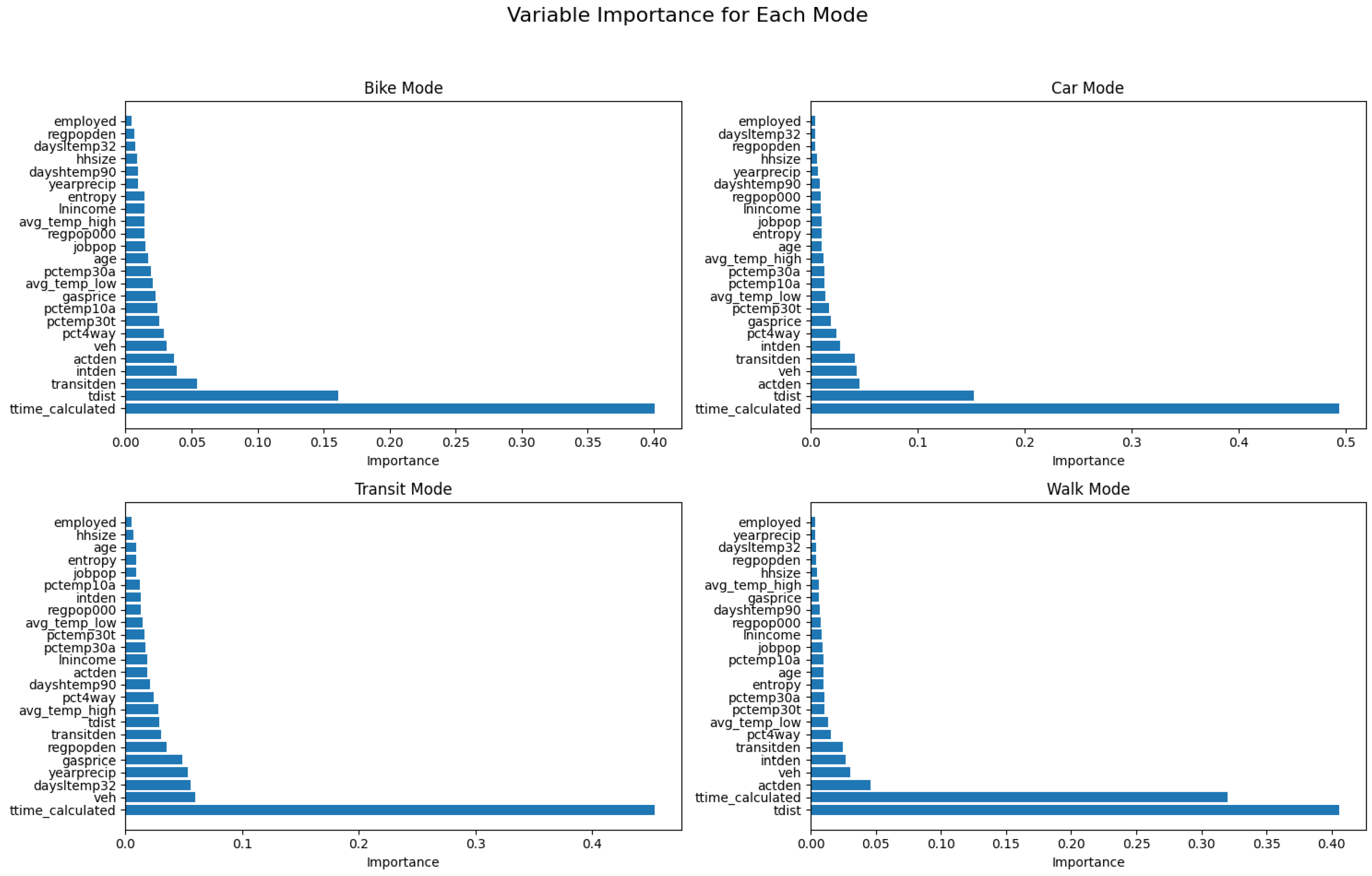
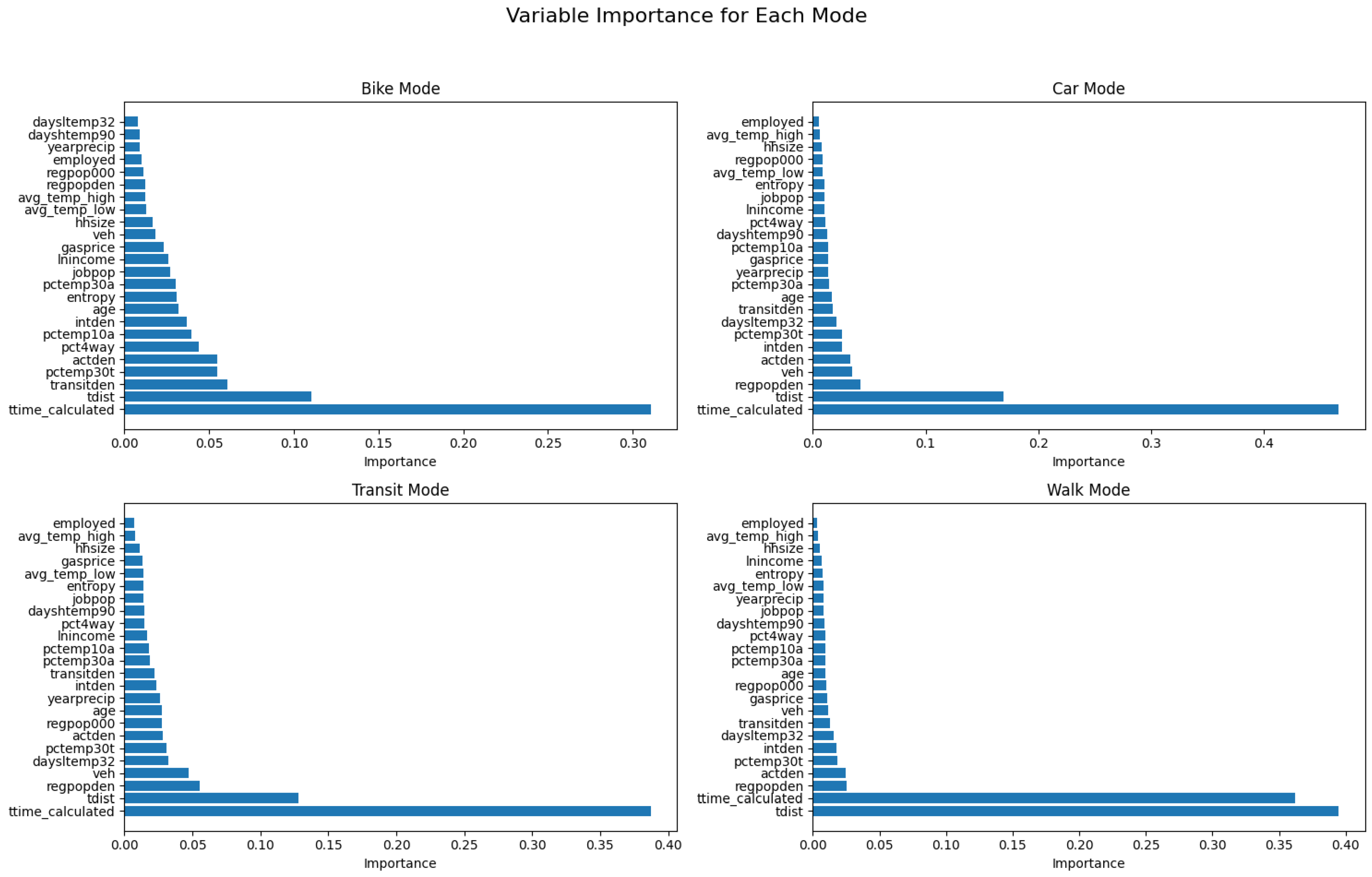
4.2. Variable Importance
5. Model Validation
- Model Generation: We generated one-vs-rest RF models for each trip purpose separately, as well as the NL model (The full report of the results of the NL model can be found in our other document, “Key Enhancements to the WFRC/MAG Four-Step Travel Demand Model”, authored by Ewing et al. (2019) [48] at the Metropolitan Research Center, University of Utah. This report is available on the NITC’s website. A summary of the NL model results tables can be found in this manuscript’s Appendix A) employed by MPOs, using the same dataset.
- Performance Measure Calculation: Performance measures were calculated for all six models (three RF and three NL models) for each transportation mode separately.
- Comparison: The performance measures were compared across the RF and NL models to ascertain the relative predictive capabilities of each.
5.1. Superior Predictive Performance
5.2. Inherent Advantages
6. Conclusions and Research Outlook
6.1. Conclusions
6.2. Research Outlook
- Investigate Barriers to Adoption: Conduct a qualitative survey among MPOs to identify the specific barriers hindering the adoption of the machine learning method, as well as the inclusion of non-motorized modes for mode choice prediction. This survey could explore technical challenges, staff expertise limitations, data availability constraints, budgetary restrictions, or even psychological resistance to new methodologies. Understanding these barriers is crucial for developing targeted strategies to promote the integration of machine learning in MPO practices.
- Demonstrate Practical Value: Develop a comprehensive communication strategy to convince MPOs of the value proposition offered by our modeling approach. This strategy could involve the following:
- ○
- Creating User-Friendly Tools: Develop user-friendly interfaces or software specifically tailored for MPOs, allowing them to easily implement and leverage the benefits of RF modeling.
- ○
- Highlighting Cost-Effectiveness: Quantify the potential cost savings and resource optimization that are achievable through more accurate predictions.
- ○
- Showcasing Real-World Applications: Develop case studies or pilot projects that demonstrate the practical benefits of RF modeling in real-world transportation planning scenarios.
Author Contributions
Funding
Institutional Review Board Statement
Informed Consent Statement
Data Availability Statement
Conflicts of Interest
Abbreviations
| MPO | Metropolitan planning organization |
| TDM | Travel demand model |
| NL | Nested logit model |
| MNL | Multinomial logit model |
| ML | Machine learning |
| RF | Random forest model |
| HBW | Home-based-Work |
| HBO | Home-Based-Other |
| NHB | Non-home-based |
Appendix A
| Variable | Estimate | Std. Error | Z Value |
|---|---|---|---|
| walk:(intercept) | −0.71305 | 0.1378 | −5.1743 *** |
| bike:(intercept) | −4.12209 | 0.3561 | −11.5741 *** |
| transit:(intercept) | −4.96735 | 0.2736 | −18.1533 *** |
| time | −0.02084 | 0.0008 | −25.1233 *** |
| walk:hhsize | 0.01614 | 0.0157 | 1.0306 |
| bike:hhsize | 0.14998 | 0.0157 | 9.5724 *** |
| transit:hhsize | 0.24468 | 0.0193 | 12.7036 *** |
| walk:veh | −0.33655 | 0.0237 | −14.2263 *** |
| bike:veh | −0.21299 | 0.0270 | −7.8911 *** |
| transit:veh | −1.26329 | 0.0314 | −40.2503 *** |
| walk:lnactden | 0.29165 | 0.0225 | 12.9439 *** |
| bike:lnactden | −0.14553 | 0.0285 | −5.1085 *** |
| transit:lnactden | 0.17849 | 0.0338 | 5.2853 *** |
| walk:pct4way | 0.00164 | 0.0008 | 2.0074 * |
| bike:pct4way | 0.00853 | 0.0009 | 9.1691 *** |
| transit:pct4way | 0.00710 | 0.0011 | 6.5861 *** |
| walk:pctemp30a | −0.00346 | 0.0014 | −2.4979 * |
| bike:pctemp30a | 0.00755 | 0.0022 | 3.4628 *** |
| transit:pctemp30a | 0.01696 | 0.0023 | 7.5079 *** |
| walk:pctemp30t | 0.00260 | 0.0018 | 1.4628 |
| bike:pctemp30t | 0.00980 | 0.0022 | 4.4542 *** |
| transit:pctemp30t | 0.00696 | 0.0025 | 2.7927 ** |
| walk:SLC Region | 0.06839 | 0.1094 | 0.6251 |
| bike:SLC Region | 2.08125 | 0.2930 | 7.1029 *** |
| transit:SLC Region | 2.54220 | 0.2134 | 11.9136 *** |
| walk:Provo-Orem Region | −0.10655 | 0.1438 | −0.7409 |
| bike:Provo-Orem Region | 2.05539 | 0.3283 | 6.2609 *** |
| transit:Provo-Orem Region | 2.28747 | 0.2673 | 8.5578 *** |
| iv:motor | 0.47541 | 0.1204 | 3.9481 *** |
| iv:nonmotor | 2.22330 | 0.0981 | 22.6641 *** |
| Number of regions: 20 Log-Likelihood: −15,989 McFadden R2: 0.33183 | |||
| Variable | Estimate | Std. Error | Z Value |
|---|---|---|---|
| walk:(intercept) | 0.47034 | 0.0359 | 13.0992 *** |
| bike:(intercept) | −2.86572 | 0.1067 | −26.8683 *** |
| transit:(intercept) | −1.94207 | 0.1152 | −16.8555 *** |
| time | −0.09814 | 0.0003 | −314.883 *** |
| walk:hhsize | −0.04072 | 0.0038 | −10.703 *** |
| bike:hhsize | −0.00680 | 0.0096 | −0.7076 |
| transit:hhsize | 0.04588 | 0.0124 | 3.7032 *** |
| walk:veh | −0.31391 | 0.0053 | −59.2256 *** |
| bike:veh | −0.16005 | 0.0132 | −12.1132 *** |
| transit:veh | −0.96448 | 0.0157 | −61.2389 *** |
| walk:pct4way | 0.00462 | 0.0003 | 17.8001 *** |
| bike:pct4way | 0.00627 | 0.0006 | 9.9308 *** |
| transit:pct4way | 0.00420 | 0.0007 | 5.7418 *** |
| walk:pctemp30t | 0.00630 | 0.0003 | 19.1271 *** |
| bike:pctemp30t | 0.00702 | 0.0009 | 8.006 *** |
| transit:pctemp30t | 0.00688 | 0.0013 | 5.2614 *** |
| walk:SLC Region | 0.46231 | 0.0351 | 13.1893 *** |
| bike:SLC Region | 0.91995 | 0.1012 | 9.0919 *** |
| transit:SLC Region | 0.29379 | 0.1194 | 2.4599 * |
| walk:Provo-Orem Region | 0.42209 | 0.0387 | 10.9028 *** |
| bike:Provo-Orem Region | 0.50353 | 0.1191 | 4.2276 *** |
| transit:Provo-Orem Region | −1.23882 | 0.2192 | −5.6528 *** |
| iv:motor | 2.72154 | 0.0445 | 61.1692 *** |
| iv:nonmotor | 1.58639 | 0.0120 | 132.2214 *** |
| iv:nonmotor | 2.22330 | 0.0981 | 22.6641 *** |
| Number of regions: 28 Log-Likelihood: −121,240 McFadden R2: 0. 34605 | |||
| Variable | Estimate | Std. Error | Z Value |
|---|---|---|---|
| walk:(intercept) | −2.87930 | 0.1081 | −26.6485 *** |
| bike:(intercept) | −3.24170 | 0.1063 | −30.5106 *** |
| transit:(intercept) | −0.24649 | 0.0148 | −16.6038 *** |
| time | −0.01123 | 0.0002 | −63.6916 *** |
| walk:hhsize | 0.02022 | 0.0064 | 3.1527 ** |
| bike:hhsize | 0.11703 | 0.0075 | 15.5387 *** |
| transit:hhsize | 0.00213 | 0.0010 | 2.1724 * |
| walk:veh | −0.06758 | 0.0097 | −6.9433 *** |
| bike:veh | −1.08760 | 0.0104 | −104.2272 *** |
| transit:veh | −0.02334 | 0.0016 | −14.6607 *** |
| walk:lnactden | 0.09354 | 0.0118 | 7.9266 *** |
| bike:lnactden | 0.27945 | 0.0122 | 22.9042 *** |
| transit:lnactden | 0.00807 | 0.0015 | 5.4579 *** |
| walk:pct4way | 0.00159 | 0.0004 | 3.7203 *** |
| bike:pct4way | 0.00068 | 0.0006 | 1.2053 |
| transit:pct4way | 0.00028 | 0.0001 | 3.8149 *** |
| walk:pctemp10a | 0.01691 | 0.0016 | 10.7216 *** |
| bike:pctemp10a | 0.00304 | 0.0016 | 1.9547 |
| transit:pctemp10a | −0.00129 | 0.0002 | −5.8653 *** |
| walk:pctemp30t | −0.00401 | 0.0006 | −6.3851 *** |
| bike:pctemp30t | 0.01752 | 0.0008 | 23.3014 *** |
| transit:pctemp30t | 0.00170 | 0.0001 | 17.4064 *** |
| walk:SLC Region | 1.02140 | 0.1066 | 9.5853 *** |
| bike:SLC Region | 0.41049 | 0.1225 | 3.3505 *** |
| transit:SLC Region | −0.05457 | 0.0187 | −2.9198 ** |
| walk:Provo-Orem Region | 1.23870 | 0.1188 | 10.4232 *** |
| bike:Provo-Orem Region | −0.76462 | 0.2214 | −3.4538 *** |
| transit:Provo-Orem Region | −0.12951 | 0.0279 | −4.6469 *** |
| iv:motor | −0.35659 | 0.0387 | −9.2133 *** |
| iv:nonmotor | 9.02280 | 0.1368 | 65.9438 *** |
| Number of regions: 28 Log-Likelihood: −104,630 McFadden R2: 0. 3757 | |||
References
- Okrah, M.B. Handling Non-Motorized Trips in Travel Demand Models. In Sustainable Mobility in Metropolitan Regions; Wulfhorst, G., Klug, S., Eds.; Studien zur Mobilitäts- und Verkehrsforschung; Springer: Wiesbaden, Germany, 2016. [Google Scholar]
- Schwartz, W.L.; Porter, C.D.; Payne, G.C.; Suhrbier, J.H.; Moe, P.C.; Wilkinson, P.C. Guidebook on Methods to Estimate Non-Motorized Travel: Overview of Methods; Cambridge Systematics, Inc.: Medford, MA, USA, 1999. [Google Scholar]
- Limtanakool, N.; Dijst, M.; Schwanen, T. The influence of socioeconomic characteristics, land use and travel time considerations on mode choice for medium-and longer-distance trips. J. Transp. Geogr. 2006, 14, 327–341. [Google Scholar] [CrossRef]
- Cervero, R. Built environments and mode choice: Toward a normative framework. Transp. Res. Part D Transp. Environ. 2002, 7, 265–284. [Google Scholar] [CrossRef]
- Wang, D.; Zhou, M. The built environment and travel behavior in urban China: A literature review. Transp. Res. Part D Transp. Environ. 2017, 52, 574–585. [Google Scholar] [CrossRef]
- Lee, J.S.; Nam, J.; Lee, S.S. Built environment impacts on individual mode choice: An empirical study of the Houston-Galveston metropolitan area. Int. J. Sustain. Transp. 2014, 8, 447–470. [Google Scholar] [CrossRef]
- Handy, S.; Cao, X.; Mokhtarian, P. Correlation or causality between the built environment and travel behavior? Evidence from Northern California. Transp. Res. Part D Transp. Environ. 2005, 10, 427–444. [Google Scholar] [CrossRef]
- Zhang, M. The Role of Land Use in Travel Mode Choice: Evidence from Boston and Hong Kong. J. Am. Plan. Assoc. 2004, 70, 344–360. [Google Scholar] [CrossRef]
- Munshi, T. Built environment and mode choice relationship for commute travel in the city of Rajkot, India. Transp. Res. Part D 2016, 44, 239–253. [Google Scholar] [CrossRef]
- Sabouri, S.; Ewing, R.; Kalantari, H.A. Estimating transit’s land-use multiplier: Direct and indirect effects on vehicle miles traveled. Transportation 2024, 1–21. [Google Scholar] [CrossRef]
- Zhang, L.; Hong, J.; Nasri, A.; Shen, Q. How built environment affects travel behavior: A comparative analysis of the connections between land use and vehicle miles traveled in US cities. J. Transp. Land Use 2012, 5, 40–52. [Google Scholar] [CrossRef]
- Khan, M.; Kockelman, K.M.; Xiong, X. Models for anticipating non-motorized travel choices, and the role of the built environment. Transp. Policy 2014, 35, 117–126. [Google Scholar] [CrossRef]
- Titze, S.; Stronegger, W.J.; Janschitz, S.; Oja, P. Association of built-environment, social-environment and personal factors with bicycling as a mode of transportation among Austrian city dwellers. Prev. Med. 2008, 47, 252–259. [Google Scholar] [CrossRef] [PubMed]
- Timperio, A.; Veitch, J.; Sahlqvist, S. Built and physical environment correlates of active transportation. In Children’s Active Transportation; Elsevier: Amsterdam, The Netherlands, 2018; pp. 141–153. [Google Scholar]
- Eldeeb, G.; Mohamed, M.; Páez, A. Built for active travel? Investigating the contextual effects of the built environment on transportation mode choice. J. Transp. Geogr. 2021, 96, 103158. [Google Scholar] [CrossRef]
- Nakshi, P.; Debnath, A.K. Impact of built environment on mode choice to major destinations in Dhaka. Transp. Res. Rec. 2021, 2675, 281–296. [Google Scholar] [CrossRef]
- Ding, C.; Wang, D.; Liu, C.; Zhang, Y.; Yang, J. Exploring the influence of built environment on travel mode choice considering the mediating effects of car ownership and travel distance. Transp. Res. Part A Policy Pract. 2017, 100, 65–80. [Google Scholar] [CrossRef]
- Chen, C.; Gong, H.; Paaswell, R. Role of the built environment on mode choice decisions: Additional evidence on the impact of density. Transportation 2008, 35, 285–299. [Google Scholar] [CrossRef]
- Cervero, R.; Kockelman, K. Travel demand and the 3Ds: Density, diversity, and design. Transp. Res. Part D Transp. Environ. 1997, 2, 199–219. [Google Scholar] [CrossRef]
- Tian, G.; Kalantari, H.A.; Ewing, R. Are older adults living in compact development more active?—Evidence from 36 diverse regions of the United States. Comput. Urban Sci. 2023, 3, 10. [Google Scholar] [CrossRef]
- Kockelman, K.M. Travel behavior as a function of accessibility, land use mixing and land use balance: Evidence from the San Francisco Bay Area. Transp. Res. Rec. 1997, 1607, 116–125. [Google Scholar] [CrossRef]
- Bento, A.M.; Cropper, M.L.; Mobarak, A.M.; Vinha, K. The impact of urban spatial structure on travel demand in the United States. Rev. Econ. Stat. 2005, 87, 466–478. [Google Scholar] [CrossRef]
- Reilly, M.; Landis, J. The Influence of Built-Form and Land Use on Mode Choice: Evidence from the 1996 Bay Area Travel Survey; University of California Transportation Center: Berkeley, CA, USA, 2002. [Google Scholar]
- Kim, B.Y.; Fleming, G.G.; Lee, J.J.; Waitz, I.A.; Clarke, J.-P.; Balasubramanian, S.; Malwitz, A.; Klima, K.; Locke, M.; Holsclaw, C.A.; et al. System for assessing Aviation’s Global Emissions (SAGE). Part 1: Model description and inventory results. Transp. Res. D 2007, 12, 325–346. [Google Scholar] [CrossRef]
- Hamre, A.; Buehler, R. Commuter Mode Choice and Free Car Parking, Public Transportation Benefits, Showers/Lockers, and Bike Parking at Work: Evidence from the Washington, DC Region. J. Public Transp. 2014, 17, 67–91. [Google Scholar] [CrossRef]
- Ferrell, C.E.; Mathur, S.; Appleyard, B.S. Neighborhood Crime and Transit Station Access Mode Choice-Phase III of Neighborhood Crime and Travel Behavior; Mineta Transportation Institute: San Jose, CA, USA, 2015. [Google Scholar]
- Bautista-Hernández, D.A. Mode choice in commuting and the built environment in México City. Is there a chance for non-motorized travel? J. Transp. Geogr. 2021, 92, 103024. [Google Scholar] [CrossRef]
- Mitra, R. School Travel Mode Choice Behaviour in Toronto, Canada. Ph.D. Thesis, University of Toronto, Toronto, ON, Canada, 2012. [Google Scholar]
- Ozbil, A.; Peponis, J. The Effects of Urban Form on Walking to Transit. In Proceedings of Eighth International Space Syntax Symposium; PUC: Santiago, Chile, 2012. [Google Scholar]
- Rajamani, J.; Bhat, C.R.; Handy, S.; Knaap, G.; Song, Y. Assessing the Impact of Urban Form Measures in Nonwork Trip Mode Choice after Controlling for Demographic and Level-of-Service Effects. In Proceedings of the Transportation Research Board Annual Meeting, Washington, DC, USA, 8 September 2003. [Google Scholar]
- Ewing, R.; Schroeer, W.; Greene, W. School Location and Student Travel Analysis of Factors Affecting Mode Choice. Transp. Res. Rec. 2004, 1895, 55–63. [Google Scholar] [CrossRef]
- Frank, L.; Bradley, M.; Kavage, S.; Chapman, J.; Lawton, T.K. Urban form, travel time, and cost relationships with tour complexity and mode choice. Transportation 2008, 35, 37–54. [Google Scholar] [CrossRef]
- Aziz, H.M.; Nagle, N.; Morton, A.; Hilliard, M.; White, D.; Stewart, R. Exploring the impact of walk–bike infrastructure, safety perception, and built-environment on active transportation mode choice: A random parameter model using New York City commuter data. Transportation 2018, 45, 1207–1229. [Google Scholar] [CrossRef]
- Cheng, L.; Chen, X.; De Vos, J.; Lai, X.; Witlox, F. Applying a random forest method approach to model travel mode choice behavior. Travel Behav. Soc. 2019, 14, 1–10. [Google Scholar] [CrossRef]
- Liu, J.; Wang, B.; Xiao, L. Non-linear associations between built environment and active travel for working and shopping: An extreme gradient boosting approach. J. Transp. Geogr. 2021, 92, 103034. [Google Scholar] [CrossRef]
- Ton, D.; Duives, D.C.; Cats, O.; Hoogendoorn-Lanser, S.; Hoogendoorn, S.P. Cycling or walking? Determinants of mode choice in the Netherlands. Transp. Res. Part A Policy Pract. 2019, 123, 7–23. [Google Scholar] [CrossRef]
- Ding, L.; Zhang, N. A Travel Mode Choice Model Using Individual Grouping Based on Cluster Analysis. Procedia Eng. 2016, 137, 786–795. [Google Scholar] [CrossRef]
- Singleton, P.A.; Clifton, K.J. Pedestrians in Regional Travel Demand Forecasting Models: State-of-the-Practice. In Proceedings of the 92nd Annual Meeting of the Transportation Research Board, Washington, DC, USA, 13–17 January 2013; pp. 13–4857. [Google Scholar]
- Zhang, Y. Microsimulating Active Transportation Mode Choice Using Smartphone-Based Travel Survey and Transportation Tomorrow Survey Data. 2015. Available online: https://tspace.library.utoronto.ca/handle/1807/71456 (accessed on 9 April 2025).
- Turner, S.; Hottenstein, A.; Shunk, G. Bicycle and Pedestrian Travel Demand Forecasting: Literature Review; Texas Transportation Institute, The Texas A&M University System: College Station, TX, USA, 1997. [Google Scholar]
- Singleton, P.A.; Totten, J.C.; Orrego-Oñate, J.P.; Schneider, R.J.; Clifton, K.J. Making strides: State of the practice of pedestrian forecasting in regional travel models. Transp. Res. Rec. 2018, 2672, 58–68. [Google Scholar] [CrossRef]
- Fehr & Peers. Model Description & Validation Report: Fresno Council of Governments Travel Demand Model. Prepared for Fresno Council of Governments, January 2014. Available online: https://www.fresnocog.org/wp-content/uploads/publications/Modeling/MIPModel_Documentation.pdf (accessed on 9 April 2025).
- Sabouri, S.; Tian, G.; Ewing, R.; Park, K.; Greene, W. The built environment and vehicle ownership modeling: Evidence from 32 diverse regions in the US. J. Transp. Geogr. 2021, 93, 103073. [Google Scholar] [CrossRef]
- Abdollahpour, S.S.; Buehler, R.; Le, H.T.; Nasri, A.; Hankey, S. Built environment’s nonlinear effects on mode shares around BRT and rail stations. Transp. Res. Part D Transp. Environ. 2024, 129, 104143. [Google Scholar] [CrossRef]
- Mohammadi, P.; Rashidi, A.; Malekzadeh, M.; Tiwari, S. Evaluating various machine learning algorithms for automated inspection of culverts. Eng. Anal. Bound. Elem. 2023, 148, 366–375. [Google Scholar] [CrossRef]
- Mohammadi, P.; Rashidi, A.; Asgari, S. Privacy-preserving culvert predictive models: A federated learning approach. Adv. Eng. Inform. 2024, 61, 102483. [Google Scholar] [CrossRef]
- Tabassum, N.; Kalantari, H.A.; Kaniewska, J.; Ameli, S.H.; Ewing, R.; Yang, W.; Promy, N.S. Ways of increasing transit ridership-lessons learned from successful transit agencies. Case Stud. Transp. Policy 2025, 19, 101362. [Google Scholar] [CrossRef]
- Ewing, R.; Sabouri, S.; Park, K.; Lyons, T.; Tian, G. Key Enhancements to the WFRC/MAG Four-Step Travel Demand Model; Transportation Research and Education Center (TREC): Portland, OR, USA, 2019. [Google Scholar]
- Azin, B.; Ewing, R.; Yang, W.; Promy, N.S.; Kalantari, H.A.; Tabassum, N. Urban Arterial Lane Width versus Speed and Crash Rates: A Comprehensive Study of Road Safety. Sustainability 2025, 17, 628. [Google Scholar] [CrossRef]

| MPO * | Area (Biggest City) | Service Area Size ** | Active Modes |
|---|---|---|---|
| BATS | Brunswick, Glynn County, Georgia | Small | No inclusion of active modes in their model. |
| RVTO | Roanoke, Virginia | Small | No inclusion of active modes in their model. |
| LMPO | Lincoln, Nebraska | Small | Employs a distance-based algorithm to estimate the proportion of non-motorized modes. Aligned with but not identical to the HBW trips, as they utilize local data which is exclusively accessible for commuting trips. Data were obtained from an external region for other trip purposes. Following an assessment of various data sources, including NHTS data, San Luis Obispo, CA, was chosen as the reference model for non-motorized modes. |
| NFRMPO | Fort Collins, Colorado | Small | Utilizing a mode choice framework that encompasses multiple multinomial choices, the NFR model divides non-motorized trips into two categories: walking and biking. Trip probabilities for these modes are determined based on their respective time allocations for walking and biking. |
| CHCNGA-TPO | Chattanooga, Catoosa Counties, Georgia | Small | ABM ***: Structured as a multinomial logit, the tour main mode sub-model offers eight mode options: Bicycle, Walk, Walk-to-Transit, Drive-to-Transit, Drive Alone, School Bus, Shared Ride (2 people), and Shared Ride (3+ people). The decision between walking or biking trips is solely based on the roundtrip road distance. |
| ARTS | Augusta, Georgia | Small | Non-motorized travel is not accounted for in the ARTS model. Instead, the mode choice component focuses on “motorized person trips”, dividing them into auto and transit trips. |
| DMAMPO | Urbandale, Iowa | Small | Mode choice modeling is not conducted by the Des Moines Area MPO. |
| StanCOG | Modesto, Stanislaus County, California | Medium | Non-motorized travel is not modeled in the StanCOG model. Instead of a comprehensive mode choice analysis step, the model utilizes an adjustment procedure. |
| COMPASS | Meridian, Idaho | Medium | A nested logit structure is employed, encompassing five alternatives. Within the non-motorized nest, walk and bicycle modes are included, with their probabilities calculated based on trip distance. |
| AMBAG | Marina, California | Medium | The mode choice model in the updated AMBAG RTDM employs a nested logit-based structure. It comprises a series of logit models, including multinomial or nested variants, which are tailored to different trip purposes and peak/off-peak periods. The model estimates probabilities for various travel modes, such as auto alone, auto-shared ride (carpool), bike, walk, and transit. Trip time and total employment density are the factors that the predictions for walk and bike trips are based on. |
| CDTC | Albany, New York | Medium | Non-motorized travel is not included in the modeling approach. The model employs a multinomial logit framework for other modes. |
| FCOG | Fresno, California | Medium | The mode choice models in Fresno County utilize a multinomial logit formulation. Within the Fresno COG Model, the mode choice step categorizes trips into various options including walking, biking, local bus, regional bus, bus rapid transit (BRT), shared ride (3+ people), shared ride (2 people), and drive alone. |
| MMPO | Memphis, Tennessee | Large | Utilizing a nested logit model, certain trip purposes do not include bike trips and are consequently excluded from consideration. The variables employed to forecast the likelihood of non-motorized trips encompass population density and household income. |
| WFRC | Salt Lake City, Utah | Large | To determine the distribution between motorized (auto and transit) trips and non-motorized trips (walk/bike), a nested multinomial logit mode choice model is employed. Trip distance is the sole predictor utilized for the non-motorized share. |
| METROPLAN | Orlando, Florida | Large | This does not model non-motorized travel. For the rest, they use a nested logit form. |
| MARC | Kansas City, Kansas and Missouri | Large | Non-motorized travel is not included in the modeling approach. The model employs a nested logit framework for other modes. |
| OKI-MPO | Cincinnati, Ohio | Large | ABM. Non-motorized travel is included in the modeling approach. The model employs a multinomial logit framework for other modes. |
| EWG | St. Louis, Missouri | Large | Non-motorized travel is not included in the modeling approach. The model employs a nested logit framework for other modes. |
| BMPO | Boston, Massachusetts | Large | The model is structured in a multinomial logit form, excluding the bike mode. Walk time serves as the sole predictor for the probability of walking |
| SEMCOG | Detroit, Michigan | Large | Non-motorized travel is not included in the modeling approach in the existing version. The model employs a multinomial logit framework for other modes. In the ongoing/future approach, utilizing ABM., the focus will extend to non-motorized transportation, delineating between walking and biking modes. This ongoing effort is projected for completion within the current year |
| TPB | Washington D.C. Metro Area | Large | No inclusion of active modes in their model. |
| H-GAC | Houston, Texas | Large | Non-motorized travel is not included in the modeling approach. The model employs a nested logit framework for other modes. |
| NCTCOG | Arlington, Texas | Large | Non-motorized travel is not included in the modeling approach. For other modes, the model employs a nested logit framework (HBW and HNW), and a multinomial logit model (NHB). |
| NJTPA | Newark, New Jersey | Large | Employing a binomial logit model, non-motorized and motorized trips are divided after trip generation but before trip distribution. However, non-motorized travel is not modeled at the mode choice stage. Nested logit is utilized for other modes. |
| CMAP | Chicago, Illinois | Large | Succeeding trip generation but preceding trip distribution, non-motorized and motorized trips are separated. However, non-motorized travel is not modeled in the mode choice model. A multinomial logit model is used for other modes. |
| Variable | Description | N | Mean | S.D. |
|---|---|---|---|---|
| Response Variables | ||||
| mode | Mode choice (categorical variable with four classes: walk, bike, transit, and car) | 807,827 | - | - |
| Trip Purpose | Trip purpose: home-based work (HBW), home-based other (HBO), non-home-based (NHB) | - | - | - |
| Trip Characteristics | ||||
| ttime_calculated | Standardized travel time | 807,827 | 0.64 | 7.85 |
| tdist | Travel distance | 807,827 | 5.7 | 1.18 |
| Households’ Socioeconomic Characteristics | ||||
| hhsize | Household size | 807,827 | 2.96 | 1.29 |
| employed | Number of employed persons in the household | 807,827 | 1.43 | 0.85 |
| veh | Number of vehicles owned by households | 807,827 | 2.1 | 1.04 |
| age | Age | 807,827 | 37.18 | 23.1 |
| lninccpe2012 | Natural log of household income (in 1000 s of 2012 dollars) | 807,827 | 11.05 | 1.26 |
| Built Environment Variables | ||||
| actden | Activity density (pop + emp per square mile in 1000 s) | 807,827 | 13.65 | 52.6 |
| Jobpop | Job–population balance | 807,827 | 0.48 | 0.31 |
| entropy | Land use entropy (mix) | 807,827 | 0.49 | 0.27 |
| Intden | Intersection density | 807,827 | 107.3 | 94.35 |
| pct4way | percentage of four-way intersections | 807,827 | 28.6 | 21.86 |
| transitden | Transit stops density (Number of stops per area) | 807,827 | 31.73 | 105.11 |
| pctemp10a | Percentage of regional employment within 10 min by auto | 807,827 | 9.21 | 13.3 |
| pctemp20a | Percentage of regional employment within 20 min by auto | 807,827 | 32.17 | 26.6 |
| pctemp30a | Percentage of regional employment within 30 min by auto | 807,827 | 54.25 | 29.5 |
| pctemp30t | Percentage of regional employment within 30 min by transit | 807,827 | 22.56 | 24.5 |
| Regional Variables | ||||
| regpop000 | Regional population in thousands | 807,827 | 3,021,449.85 | 1,783,604 |
| regpopden | Regional population density | 807,827 | 791.18 | 377.13 |
| gasprice | Regional gas price | 807,827 | 2.87 | 0.11 |
| avg_temp_low | Annual average of low temperature | 807,827 | 38.79 | 13.23 |
| avg_temp_high | Annual average of high temperature | 807,827 | 74.75 | 8.31 |
| daysltemp32 | Number of days of low temperature <= 32 °F | 807,827 | 35.54 | 39.36 |
| dayshtemp90 | Number of days of high temperature >= 90 °F | 807,827 | 46.63 | 43.61 |
| yearprecip | Annual precipitation in inches | 807,827 | 40.39 | 15.11 |
| Performance Measure | HBW | HBO | NHB | |||
|---|---|---|---|---|---|---|
| RF | NL | RF | NL | RF | NL | |
| AUC-ROC | 0.997 | 0.637 | 0.99 | 0.807 | 0.98 | 0.914 |
| Accuracy | 0.984 | 0.936 | 0.99 | 0.90 | 0.974 | 0.865 |
| Balanced Accuracy | 0.95 | 0.584 | 0.97 | 0.64 | 0.94 | 0.75 |
| F1 | 0.983 | 0.43 | 0.993 | 0.76 | 0.993 | 0.76 |
| Recall | 0.984 | 0.27 | 0.998 | 0.61 | 0.993 | 0.83 |
Disclaimer/Publisher’s Note: The statements, opinions and data contained in all publications are solely those of the individual author(s) and contributor(s) and not of MDPI and/or the editor(s). MDPI and/or the editor(s) disclaim responsibility for any injury to people or property resulting from any ideas, methods, instructions or products referred to in the content. |
© 2025 by the authors. Licensee MDPI, Basel, Switzerland. This article is an open access article distributed under the terms and conditions of the Creative Commons Attribution (CC BY) license (https://creativecommons.org/licenses/by/4.0/).
Share and Cite
Kalantari, H.A.; Sabouri, S.; Brewer, S.; Ewing, R.; Tian, G. Machine Learning in Mode Choice Prediction as Part of MPOs’ Regional Travel Demand Models: Is It Time for Change? Sustainability 2025, 17, 3580. https://doi.org/10.3390/su17083580
Kalantari HA, Sabouri S, Brewer S, Ewing R, Tian G. Machine Learning in Mode Choice Prediction as Part of MPOs’ Regional Travel Demand Models: Is It Time for Change? Sustainability. 2025; 17(8):3580. https://doi.org/10.3390/su17083580
Chicago/Turabian StyleKalantari, Hannaneh Abdollahzadeh, Sadegh Sabouri, Simon Brewer, Reid Ewing, and Guang Tian. 2025. "Machine Learning in Mode Choice Prediction as Part of MPOs’ Regional Travel Demand Models: Is It Time for Change?" Sustainability 17, no. 8: 3580. https://doi.org/10.3390/su17083580
APA StyleKalantari, H. A., Sabouri, S., Brewer, S., Ewing, R., & Tian, G. (2025). Machine Learning in Mode Choice Prediction as Part of MPOs’ Regional Travel Demand Models: Is It Time for Change? Sustainability, 17(8), 3580. https://doi.org/10.3390/su17083580