The Heterogeneous Relationship Between China’s Low-Carbon Economic Scale and Quality: A County-Level Analysis from the Perspective of Administrative Division

Abstract

Under China’s ambitious “Dual Carbon” strategy, understanding the relation hip between the scale and quality of the low-carbon economy at the county level is crucial for providing robust empirical evidence to guide policymakers. This study employs panel vector autoregression, panel fixed-effects regression, and panel multinomial logit regression to explore the heterogeneous relationship between scale and quality across counties and municipal districts, as well as to investigate the underlying mechanisms. The findings reveal that (1) county-level quality growth has a statistically significant positive effect on scale growth, indicating that China’s current low-carbon development strategy, with its emphasis on quality improvement, is well-timed; (2) although scale growth negatively impacts quality growth at the county level, this effect is not significant in municipal districts; (3) the development of the secondary industry, large-scale industrial output intensity, and resource-based development contribute to the heterogeneous relationship between scale and quality; and (4) emission reduction technology and local government intervention significantly enhance quality in municipal districts more than in counties, primarily by influencing the degree of decoupling.

1. Introduction

Amid the growing global sustainability discourse, the influential 2003 UK Energy White Paper “Our Energy Future: Creating a Low Carbon Economy” formally established the term “low-carbon economy” in policy discourse, significantly advancing international climate policy development. The modern low-carbon economic paradigm exhibits dual core characteristics: firstly, it reduces fossil fuel dependence and carbon intensity through clean energy system transformation (e.g., increased renewable energy penetration and widespread adoption of energy-efficient technologies); secondly, it maintains medium-to-high economic growth under environmental constraints via innovation-driven development pathways, including industrial structure upgrading and commercialization of green technologies. This “emission reduction-growth” synergy mechanism has been widely recognized as a crucial strategy in climate governance, with the United Nations Environment Programme emphasizing its pivotal role in sustainable development transformations [1,2]. Therefore, enhancing the quality and widening the scale of the low-carbon economy are two critical aspects [3,4]. However, Chen et al. [5] argued that the quality and scale of countries’ low-carbon economies cannot be easily and simultaneously achieved, especially in developing countries. In response to the Kyoto Protocol and the Paris Agreement, sacrificing economic growth to reduce CO₂ emissions or compromising the environment to stimulate GDP growth is a difficult choice faced by many countries and regions [6]. In particular, compared with developed countries, reducing poverty and mitigating climate change are two major challenges facing developing countries. It is evident that the economic growth of developing countries often relies on excessive consumption of resources and environmental degradation, but it is also beneficial for absolute poverty reduction and increases in social welfare. In the context of low-carbon economic development, discussions on the low-carbon economy must be based on a holistic perspective. For example, a related issue is whether there is a trade-off between low-carbon economic scale and quality [5]. However, existing studies are often limited to exploring the quality of the low-carbon economy, such as its spatiotemporal variation and determinants [3,7,8], which may hinder the development of more comprehensive and targeted policy implications for achieving sustainable development.

It is worth emphasizing that the relationship between China’s low-carbon economic scale and quality requires more attention, given that it will provide important empirical evidence on how other developing countries can achieve coordinated development of scale and quality. As a major global carbon emitter, China has set ambitious targets for achieving its “Dual Carbon” strategy. However, it should not be ignored that China is still the world’s largest developing country, which continues to prioritize economic development and poverty eradication. Achieving the “Dual Carbon” strategy while ensuring high-quality and large-scale economic growth is a significant challenge for the Chinese government. Particularly, after China’s economy entered the “new normal”, improving quality and stabilizing growth have become China’s new development goals. Therefore, the relationship between scale and quality requires more attention to provide more empirical evidence for policymakers to propose and implement more targeted strategies for the goals of “Dual carbon” strategy.

As the basic administrative unit of policy implementation in China, municipal districts and counties play a crucial role in carrying out the directives of the central government and formulating specific action plans. Thus, China’s county-level low-carbon economy needs to be discussed to propose targets for more sustainable and stable development. For example, in the traditional economic growth pattern, many county-level regions’ development was at the expense of environmental quality. In this case, local governments may forcibly shut down high-emission enterprises within their jurisdiction to achieve emission reduction targets, negatively impacting local economic growth. Therefore, it is of great practical significance to pay more attention to the relationship between scale and quality at the county level. Moreover, given that China’s county-level regions are usually divided into counties and municipal districts based on different stages of industrial structure, urbanization rates, and population aggregation, it is significant to explore their differences in terms of low-carbon economic development.

However, few studies have investigated China’s low-carbon economic scale and quality at the county level. Addressing this gap, we made use of satellite data to assess the scale and quality of the low-carbon economy across county-level regions. Next, the panel vector autoregression analysis was employed to conduct impulse-response analysis between scale and quality across counties and municipal districts to reveal their heterogeneous causal relationship. Moreover, to offer robust and insightful recommendations for achieving high quality while maintaining stable scale growth, the underlying causes of the variation across counties and municipal districts were examined through the lenses of industrial structure, emission reduction technology, and local government intervention.

Specifically, this study makes several key contributions: (1) our study makes an important contribution to the existing literature by revealing important insights into the scale and quality characteristics of China’s county-level low-carbon economies; (2) we discussed the heterogeneous relationship between scale and quality across counties and municipal districts, as is beneficial for proposing robust and insightful suggestions for Chinese county-level policymakers; and (3) our empirical evidence may also provide useful information on how other developing countries can achieve coordinated development of low-carbon economic scale and quality.

2. Literature Review

In light of the existing literature, numerous studies have evaluated China’s low-carbon economy in terms of scale and quality [5,8]. Regarding the scale, absolute indicators (e.g., low-carbon economic output and green GDP) have been used to reflect the quantitative characteristics of low-carbon economy [9,10,11,12]. Compared to traditional GDP statistics, absolute indicators account for the costs of CO₂ emissions [13]. Although low-carbon GDP measures quantity, a region with high economic output and CO₂ emissions may still have a high low-carbon GDP if the carbon price is low. Consequently, many studies have adopted relative carbon intensity to assess the quality of this low-carbon economy [14,15,16,17]. In addition to carbon intensity, the proportion that low-carbon GDP (or green GDP) occupies in total GDP has also been incorporated to quantify the quality of low-carbon economy [5,13,18]. Compared to carbon intensity, this index takes into account the economic costs and revenues associated with CO₂ emissions and sequestration, thereby better distinguishing green economic output from conventional output.

To date, the existing literature predominantly focuses on either the scale or quality of China’s low-carbon economy, with few studies addressing their relationship [17,19]. Furthermore, research in this field has primarily focused on the national and provincial levels, with insufficient attention given to county-level analyses due to data availability limitations. Given that county-level units play a crucial role in policy formulation and implementation, further exploration of the relationship at the county level is of significant importance.

Addressing this literature gap, this study measures China’s county-level low-carbon economic scale (quantified by low-carbon GDP) and quality (quantified by the proportion of low-carbon GDP to GDP), consistent with previous studies [5,8]. Subsequently, we employed panel vector autoregression analysis to explore the relationship between scale and quality. In particular, the heterogeneity in the relationship between scale and quality across counties and municipal districts was explored. Additionally, the potential reasons were discussed from the perspectives of industrial structure, emissions reduction technology, and local administrative intervention.

3. Materials and Methods

3.1. Theoretical Background and Hypothesis

Based on the scale perspective of the Environment Kuznets Curve (EKC) theory [20,21,22,23], we deduce that, at the county level, there may be a potential nonlinear relationship between scale and quality. Therefore, the first hypothesis is proposed as follows:

Hypothesis 1.

Improving low-carbon economic quality in China is timely, which also made positive contributions to scale growth at the county level.

According to China’s definitions of county-level administrative divisions, a county can be upgraded to a municipal district only when it has reached high levels of economic status, service industry development, and technological innovation. Since many counties’ economic growth is more dependent on highly polluting industries than that of municipal districts’, counties are more likely to be in the earlier stage of the EKC. Hence, there may be heterogeneity in the response of quality growth to scale growth across counties and municipal districts. Hence, the second hypothesis is proposed as follows:

Hypothesis 2.

Given the different economic statuses of counties and municipal districts, there may be a heterogeneous relationship between China’s low-carbon economic scale and quality across counties and municipal districts.

Based on the structure effect of the EKC, the industrial structure, technological advancement, and local government intervention may help achieve the decoupling of scale growth and CO₂ emissions so as to promote the quality [22,24,25,26,27,28,29,30,31,32]. Since counties and municipal districts have different statuses in terms of these variables, the third hypothesis is proposed as follows:

Hypothesis 3.

Secondary industry development, emission reduction technological progress, and local administrative intervention were responsible for the heterogeneity in counties and municipal districts.

3.2. Empirical Models

In this study, we employ the panel vector autoregression (PVAR), panel fixed-effect regression, and panel multinomial logit regression methods to investigate the heterogeneous relationship between scale and quality across counties and municipal districts, as well as the potential mechanisms. And the research roadmap is presented as follows (see Figure 1):

Following previous studies [33,34,35], the PVAR approach was adopted with the purpose of investigating how the scale (or quality) will respond to the shock of quality (or scale). Following [5,36], neo (low-carbon GDP), reo (the proportion of low-carbon GDP to GDP), and energy consumption (e) were incorporated as endogenous variables. The specific reasons for the selection include two aspects: (1) much of the existing literature has confirmed that a reciprocal causal relationship exists between neo and reo; (2) in light of previous studies, there is always a causal relationship between energy consumption and economic growth [6,33,37]. If the carbon price is low, neo is highly correlated with economic output. And energy consumption is an important driver of economic output. So, neo may respond to the shock of energy consumption [38]. Hence, this study proposes the baseline model as follows:

$$\mathsf{\Delta }\mathrm{l}\mathrm{n}{(Z}_{i,t})=a_0+a_1\mathsf{\Delta }\mathrm{l}\mathrm{n}{(Z}_{i,t-1})+a_2\mathsf{\Delta }\mathrm{l}\mathrm{n}\left(Z_{i,t-2}\right)+...+a_j\mathsf{\Delta }\mathrm{l}\mathrm{n}{(Z}_{i,t-j})+{\mu }_i+{\phi }_t+{\epsilon }_{it}$$

(1)

where $\mathsf{\Delta }\mathrm{l}\mathrm{n}{(\mathrm{Z}}_{\mathrm{i},\mathrm{t}})$ represents a 1 × 3 vector of the logarithmic form of three endogenous variables: ln(reo), ln(neo) and ln(e). Based on the Bayesian Information Criterion (BIC), we selected the optimal lag-length. The BIC criterion strictly penalizes the complexity of parameters and gives priority to selecting simpler lag orders, thereby avoiding overfitting in PVAR models, which has been widely adopted in many studies [39]. It is particularly applicable to large sample sizes and theory-driven analyses, and its adaptability to panel data can strike a balance between individual heterogeneity and dynamic robustness. The optimal lag order under the BIC criterion can be obtained through the official command integrated in Stata software 17.0 for calculation. At the same time, this study checked the stationarity of the variables and the stability of the system. Additionally, confidence interval bands were generated based on 1000 Monte Carlo simulations. Moreover, the granger casual test and generalized impulse responses were employed to explore the link between the scale and quality in counties and municipal districts, respectively.

Further, in light of the theoretical analysis and hypotheses proposed above in Section 3.1, the effects of industrial structure on counties’ and municipal districts’ reo were analyzed. The baseline model is presented as follows:

$$\mathrm{l}\mathrm{n}\left(re{o}_{it}\right)=a_0+a_1\mathrm{l}\mathrm{n}\left(IN{D}_{it}\right)+a_{x}contro{l}_{it}+{\mu }_i+{\gamma }_t+{\epsilon }_{it}$$

(2)

where $\mathrm{l}\mathrm{n}\left(IN{D}_{it}\right)$ denotes the logarithmic form of industrial structure, which is represented by the ratio of secondary industry’s output (ln(is)) and the proportion of large-scale industrial output to GDP (ln(ii)). With regard to the control variables, we incorporated economic development level (ln(gdppercapita)), emission reduction technological progress (ln(ctfp)), carbon density (ln(ce)), industrial structure (ln(is)), population density (ln(poparea)), land urbanization (ln(u)), net primary productivity (ln(npp)), the ratio of forested areas to the total land area (ln(ratio)), financial development level (ln(fe)), government intervention (ln(gove)), and regional targets for energy conservation and emission reduction (T1, T2, and T3) as control variables, which are consistent with previous studies [8,39,40,41]. And fixed effects (FEs) were applied in this study to analyze the panel data.

As for the influences of emission reduction technology and local government intervention on the low-carbon economy, their effect on the marginal probability of decoupling was studied based on the panel multinomial logit model. In particular, we adopted the Tapio decoupling elasticity index [42] to estimate the decoupling elasticity at the county level. Next, a dummy variable (tapio) was constructed as the explained variable based on whether CO₂ emissions decoupled from economic growth in county-level regions (tapio = 1 denotes that the county-level regions achieved strong or weak decoupling, and 0 otherwise). Following previous studies [43,44,45], the panel multinomial logit model was developed based on the following equations, which are consistent with [46].

$$tapi{o}_{it}=a_0+a_1\mathrm{l}\mathrm{n}\left(ctf{p}_{it}\right)+a_2\mathrm{l}\mathrm{n}\left(gov{e}_{it}\right)+a_{x}contro{l}_{it}+{\mu }_i+{\gamma }_t+{\epsilon }_{it}$$

(3)

$$\begin{array}{ll}& P\left(tapi{o}_{it}=1\mid X_{it},{\mu }_i,{\gamma }_t\right)=P\left(tapi{o}_{it}>0\mid X_{it},{\mu }_i,{\gamma }_t\right)\\ & =P\left({\alpha }_0+{\alpha }_1\mathrm{l}\mathrm{n}\left(ctf{p}_{it}\right)+{\alpha }_2\mathrm{l}\mathrm{n}\left(gov{e}_{it}\right)+{\alpha }_{x}contro{l}_{it}+{\mu }_i+{\gamma }_t+{\epsilon }_{it}>0|X_{it},{\mu }_i,\gamma \right)\\ & ={\displaystyle \frac{Exp\left(a_0+a_1\mathrm{l}\mathrm{n}(ctf{p}_{it)}+a_2\mathrm{l}\mathrm{n}(gov{e}_{it})+a_{x}contro{l}_{it}+{\mu }_i+{\gamma }_t+{\epsilon }_{it}\right)}{1+Exp\left(a_0+a_1\mathrm{l}\mathrm{n}\left(ctf{p}_{it}\right)+a_2\mathrm{l}\mathrm{n}\left(gov{e}_{it}\right)+{\alpha }_{x}contro{l}_{it}+{\mu }_i+{\gamma }_t+{\epsilon }_{it}\right)}}\end{array}$$

(4)

where ln(ctfp) represents emission reduction technological progress, which was estimated based on the production-theoretical decomposition analysis (PDA) approach; and ln(gove) represents local government intervention. Following previous studies [46,47,48,49], it was measured as the proportion of local general budget expenditure to GDP. And control_i,t was consistent with model (2).

Moreover, to explore the impacts of ln(ctfp) and ln(gove) on the ln(reo) through the degree of decoupling, the cross-terms of ln(ctfp) (or ln(gove)) and the dummy variable (tapio) were incorporated into model (2). Finally, the models are presented as follows:

$$\begin{array}{ll}& \mathrm{l}\mathrm{n}\left(re{o}_{it}\right)=a_0+a_1\mathrm{l}\mathrm{n}\left(ctf{p}_{it}\right)+a_2\mathrm{l}\mathrm{n}\left(ctf{p}_{it}\right)\times i.tapio+a_{3}i.tapio\\ & +a_{x}contro{l}_{it}+{\mu }_i+{\gamma }_t+{\epsilon }_{it}\end{array}$$

(5)

$$\begin{array}{ll}& \mathrm{l}\mathrm{n}\left(re{o}_{it}\right)=a_0+a_1\mathrm{l}\mathrm{n}\left(gov{e}_{it}\right)+a_2\mathrm{l}\mathrm{n}\left(gov{e}_{it}\right)\times i.tapio+a_{3}i.tapio\\ & +a_{x}contro{l}_{it}+{\mu }_i+{\gamma }_t+{\epsilon }_{it} \end{array}$$

(6)

In particular, the cross-terms help reveal the impacts of ln(ctfp) and ln(gove) under the stages of strong or weak decoupling, reflecting the action channel of the degree of decoupling.

3.3. Evaluation of Scale and Quality Using Satellite Data

Based on the ideas of [5,13,25], neo and reo can be utilized to assess the scale and quality of the low-carbon economy. Accordingly, neo and reo were selected by us as key metrics to evaluate the low-carbon economy in China at the county level. In line with previous studies [5], neo and reo were estimated using Equation (7).

$$\begin{array}{lll}& & re{o}_i^t={\displaystyle \frac{ne{o}_i^t}{Y_i^{*t}}}\\ & & \\ & & ={\displaystyle \frac{Y_i^{*t}+P\times \left(C{S}_i^t-C_i^t\right)}{Y_i^{*t}}}\end{array}$$

(7)

where $Y_i^{*t}$ denotes real GDP; according to the IPCC [5,50], $P$ denotes the CO₂ emission price at the projected steady-state value of USD 80 per metric ton; $C{S}_i^t$ represents forest carbon sequestration; and $C_i^t$ represents energy-related CO₂ emissions.

Compared with other indicators typically employed in previous studies [51,52,53,54,55], such as carbon intensity or carbon productivity, reo takes into account real GDP growth calibrated and forest carbon sequestration adjustments, providing a more comprehensive evaluation of the low-carbon economy in the context of the “Dual Carbon” strategy.

3.4. Data Sources

Due to data-availability constraints, this study focuses on 1674 county-level administrative units in China, covering the period from 2001 to 2018. To ensure accurate classification, we strictly adhere to the administrative criteria outlined in the “China County (City) Statistical Yearbook”, which defines counties based on whether the State Council has officially designated them as municipal districts. Additionally, due to the relatively small geographical size of some municipal districts (particularly urban core districts), their boundaries cannot be reliably extracted from coarse-resolution gridded datasets. Therefore, we consolidate all districts within the same prefecture-level city into a single analytical unit.

Regarding data sources, CO₂ emission data are sourced from a globally recognized gridded emissions database [56], which adopts a bottom-up accounting methodology covering all EDGAR-defined sectors (e.g., energy, industry, and transportation). Its aggregated provincial and national estimates align closely with official statistics. Forest carbon sequestration data are obtained from the high-resolution global carbon stock dataset developed by Harris et al. [57] that integrates multi-sensor remote sensing and ground observations to improve spatiotemporal accuracy. County-level energy consumption data are sourced from Chen et al. [5], who used a calculation method similar to that of Lv et al. [58].

Real GDP dataset was obtained from Chen et al. [59], which corrects traditional GDP statistics by integrating NTL data and land-use information, significantly enhancing county-level economic data reliability. For urbanization measurement, due to the unavailability of urban population data at the county level, we use the built-up area ratio (derived from NASA’s 500 m resolution MCD12Q1 land cover product) as a proxy, a well-validated approach in prior studies [60,61]. Forest cover is calculated by summing five forest types (evergreen needleleaf, evergreen broadleaf, deciduous needleleaf, deciduous broadleaf, and mixed forests) from the same MCD12Q1 product. Vegetation productivity is represented by net primary productivity (NPP) estimates from the MOD17A3H product [62]. Population data are sourced from the high-accuracy WorldPop project (2013 edition). Socioeconomic variables are obtained from China’s official statistical data.

4. Results and Discussion

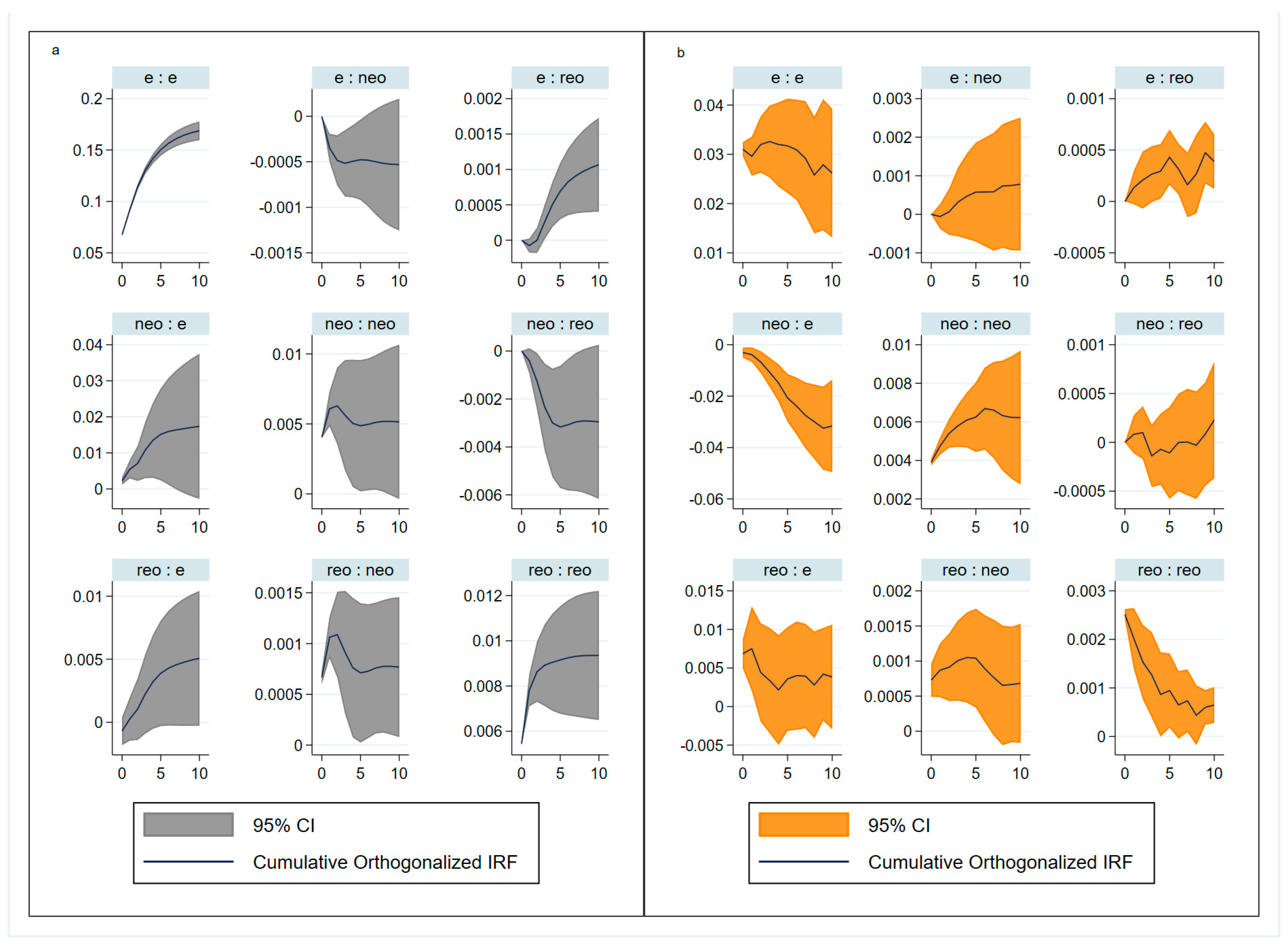
4.1. Different Relationship Between Scale and Quality Across Counties and Municipal Districts

This study aims to systematically examine the intrinsic relationship between the scale and quality of low-carbon economic development at the county level. To meet the requirements of panel data analysis, we constructed a panel vector autoregression (PVAR) model system incorporating multidimensional indicators. Prior to model estimation, strictly following standard econometric procedures [5,63], we conducted rigorous stationarity diagnostics using two representative panel unit root tests—the Im–Pesaran–Shin (IPS) test and the Levin–Lin–Chu (LLC) test on all relevant economic and environmental indicators. The test results confirmed the stationarity of all variables, thus ensuring the validity of our empirical analysis and enhancing the robustness of policy recommendations derived from the research findings (see

Table 1. IPS and LLC panel unit root tests for logarithmic variables in PVAR analysis across continents.

Region	Variables	IPS Test	LLC Test
Counties	dln(reo)	−55.29 ***	−72.54 ***
	dln(neo)	−56.30 ***	−110 ***
	dln(e)	−53.07 ***	−45.05 ***
Municipal districts	dln(reo)	−25.65 ***	−300 ***
	dln(neo)	−26.18 ***	−62.21 ***
	dln(e)	−23.70 ***	−10.07 ***

Notes: ***, **, and * denote significance at the 1%, 5%, and 1% levels, respectively.

).

Subsequently, based on the stability of the system, Granger causal relationships among these variables were discussed, and they are presented in Appendix A 

Table A1. Panel Granger causal relationship.

	Counties	Municipal Districts
dln(neo)$\to$dln(reo)	23.04 ***	59.59 ***
dln(e)$\to$dln(reo)	57.07 ***	65.03 ***
dln(neo)+dln(e)$\to$dln(reo)	119.59 ***	128.54 ***
dln(reo)$\to$dln(neo)	15.93 ***	34.05 ***
dln(e)$\to$dln(neo)	56.59 ***	73.82 ***
dln(reo)+dln(e)$\to$dln(neo)	85.59 ***	113.16 ***
dln(reo)$\to$dln(e)	16.10 ***	43.52 ***
dln(neo)$\to$dln(e)	70.54 ***	57.17 ***
dln(neo)+dln(reo)$\to$dln(e)	90.91 ***	109.11 ***

Notes: ***, **, and * denote significance at the 1%, 5%, and 1% levels, respectively.

. It shows that neo growth, reo growth, and e growth are Granger-causally related to each other. Hence, the long-term responses to shocks of each variable to others can be simulated.

Figure 2 reports the generalized impulse responses of counties and municipal districts (empirical confidence bands computed via 1000 Monte Carlo iterations), which helps reveal the response of neo (or reo) and to a shock on reo (or neo). At the same time, we employed cumulative impulse responses to identify the long-term effects. It shows that an increase in reo had a statistically significant positive impact on neo growth in counties and municipal districts (with a 95% confidence), while neo growth failed to promote reo growth in counties and municipal districts. Chen et al. [5] also drew the same conclusion based on panel data for 77 countries during 2001–2019. Similarly, Li and Wei [27] also found that reductions in CO₂ emissions facilitated economic performance improvement. It follows that China’s current low-carbon development strategy, aimed at improving quality, is timely and will not threaten economic scale in the long term.

In particular, the impact of neo growth on reo growth varied across counties and municipal districts. Specifically, neo growth in counties had a negative impact on reo growth at the 95% confidence interval, but an increase in neo in municipal districts had no significant impact on reo growth. According to the theory of EKC, the industrial structure and energy consumption structure significantly affect the dependence between economic growth and environmental quality [64,65]. Considering that the economic growth of counties is more dependent on highly polluting industries than that of municipal districts, their scale growth leads to a decline in environmental quality. Additionally, to address the potential bias caused by administrative boundary adjustments, we re-conducted the analysis after excluding counties that experienced jurisdictional changes from 2001 to 2018. The results remained consistent (see Appendix B Figure A1).

To further identify specific counties that exhibited a negative influence of neo growth on reo growth, this study adopted a subsample of counties to conduct panel vector autoregression analysis in terms of industrial structure and energy use structure, as is consistent with the existing studies [5,17,66,67]. Specifically, following [8,67], carbon density (i.e., the ratio of CO₂ emissions to energy consumption) was adopted to indirectly reflect energy consumption structure given that county-level energy-balance tables are not available. Figure 3a,b report that neo growth only had exerted negative influence on reo growth in counties in the highest quartile of carbon density (which was sorted from smallest to largest).

Similarly, Figure 4a,b also show that the negative influence of neo growth on reo growth only occurred in counties with a high quartile of secondary industry output share. The results imply that if counties that rely on the secondary industry do not rapidly upgrade their industrial structure, the quality of their low-carbon economy will continue to decline when economic scale increases, which is not conducive to the realization of “carbon peak” and “carbon neutrality”. Therefore, industrial structure and energy consumption structure may be important factors affecting the relationship between China’s county-level scale and quality.

Moreover, the classification of key and non-key environmental-protection cities was employed to obtain a subsample of resource-based counties. The classification is based on previous studies [68]. The cumulative generalized impulse responses are presented in Figure 5. Compared with non-resource-based counties, we found that reo growth of resource-based counties suffered from a more serious risk of decline when neo increased. According to [69], China’s regional resource-based development is associated with high ratios of mining and manufacturing, thus leading to a negative response of reo growth to neo growth.

4.2. Robustness Checks

To enhance the robustness of our findings regarding the differences between counties and municipal districts (as established in Section 3.1), we implemented multiple validation measures to confirm the reliability of our empirical results.

4.2.1. Substitute Variables

First, we verified the robustness of impulse-response results based on the substituted variables. Many scholars have employed carbon intensity to reflect the quality of low-carbon economy [15,70]. Thus, we replaced reo and neo to validate the robustness of our conclusions. In particular, reo was substituted by carbon intensity (ci), and neo was substituted with GDP (y). Evidently, reo is negatively associated with carbon intensity, and y is positively associated with neo.

Figure 6 reports the generalized impulse responses analysis in counties and municipal districts. The results show that the increase (or decrease) of ci growth can lead to the decrease (increase) of y growth, as well as neo growth. Heterogeneous effects of GDP growth on carbon intensity growth also exist across counties and municipal districts. Specifically, y growth in municipal districts decreased their ci growth, while counties’ GDP failed to reduce carbon intensity. The results indicate that the development of counties’ economic output cannot achieve a decline in carbon intensity, and thus they have failed to enhance the quality. In conclusion, although carbon intensity does not consider the effects of forest carbon sequestration, similar conclusions are still obtained after replacing the reo index and neo index, thus verifying the robustness of the previous analysis.

4.2.2. Omitted Variables

China’s rapid urbanization has emerged as a crucial driver of low-carbon economic development [40,41]. To examine this relationship more comprehensively, we incorporated land urbanization (u) as an endogenous variable in our analysis of the scale-quality dynamics across counties and municipal districts. As illustrated in Figure 7, the results reveal several key findings: (1) reo growth consistently promotes neo growth in both administrative units; (2) a neo increase exerts significantly negative effects on reo growth in counties with high carbon density and secondary industry output ratios, though this pattern is absent in municipal districts; and (3) the inclusion of u yields cumulative generalized impulse responses that align with our baseline results, thereby reinforcing the robustness of our conclusions.

4.2.3. Discussion on Nonlinear Relationship Based on Fixed Effects Panel Regression Analysis

After adding land urbanization to the panel vector autoregression analysis, this study obtained the same conclusions. However, the number of variables that can be set as endogenous variables is limited. The effects of neo on counties’ and municipal districts’ reo can be influenced by some omitted factors. To address this issue, the study employs a two-way fixed effects panel regression approach to analyze the nonlinear relationship between reo and neo across counties and municipal districts. The results are shown in

Table 2. Robustness-check results based on discussions on the nonlinear relationship.

	(1)	(2)	(3)	(4)
	ln(reo)	ln(reo)	ln(reo)	ln(reo)
	Counties	Municipal districts	Counties with high quartiles of ln(ce)	Counties with high quartiles of ln(is)
ln(neo)	−0.4296 ***	−1.8998 ***	−0.0465	0.3654
	(0.0694)	(0.5676)	(0.1466)	(1.3301)
ln(neo2)	0.0215 ***	0.1038 ***	−0.0083	−0.0257
	(0.0048)	(0.0321)	(0.0116)	(0.0816)
Control variables	Yes	Yes	Yes	Yes
Lower bound slope	−0.18	−0.72 ***	−0.14	0.075
Upper bound slope	−0.0006	0.17 **	−0.21	−0.14
Individual FE	Yes	Yes	Yes	Yes
Year FE	Yes	Yes	Yes	Yes
R2	0.1200	0.2051	0.3560	0.3368
N	12,616	3056	3157	2929

Notes: (a) ***, **, and * denote significance at the 1%, 5%, and 1% levels, respectively; and (b) values in parentheses denote robust standard errors.

, and the “utest command” in the Stata module was used to examine the presence of a U-shaped relationship over an interval in this study, which is consistent with [71,72].

Columns (1) and (2) present that the coefficients of ln(neo2) are significantly positive in counties and municipal districts. The nonlinear tests show that the curve only takes the expected U-shape in municipal districts, while it is not significant in counties. Moreover, the coefficients of ln(neo2) in counties with high quartiles of ln(ce) (quantified by carbon density) and ln(is) (quantified by the ratio of secondary industry’s output to GDP) are insignificant (see columns (3) and (4)). Since the economic level of municipal districts is much higher than that of counties, they have constantly realized the upgrading of the industrial structure, thus gradually cutting CO₂ emission growth, along with economic growth. However, counties always rely more on highly polluting industries, causing a decline in quality. In summary, our fixed-effects panel regression analysis further confirmed that the negative influence of neo growth on reo growth only occurs in counties.

4.3. Explorations on the Potential Reasons

Although the cumulative generalized impulse response analysis reveals the heterogeneity across counties and municipal districts, the potential reasons are still unclear. EKC argues that structural and technological effects are major factors contributing to the nonlinear relationship between economic growth and polluting emissions. Simultaneously, many previous studies found that industrial structure, technological progress, and administrative intervention are important driving factors affecting low-carbon economy [5,21,40]. Thus, this study further investigated the potential reasons why heterogeneous impulse responses exist across counties and municipal districts from the aspect of industrial structure, technology, and administrative intervention.

4.3.1. The Different Impacts of Secondary Industry Development and Large-Scale Industrial Development Across Counties and Municipal Districts

According to Gao [8], ln(is) and ln(ii) can be employed to reflect the characteristics of industries with high CO₂ emissions.

Table 3. The different impacts of industrial structure on ln(reo) across counties and municipal districts.

	(1)	(2)	(3)	(4)
	ln(reo)	ln(reo)	ln(reo)	ln(reo)
	Counties	Municipal districts	Counties	Municipal districts
ln(is1)	−0.0063 **	−0.0211
	(0.0026)	(0.0138)
ln(is2)			−0.0026 **	−0.0013
			(0.0011)	(0.0070)
Control variables	Yes	Yes	Yes	Yes
Individual FE	Yes	Yes	Yes	Yes
Year FE	Yes	Yes	Yes	Yes
R2	0.1055	0.1293	0.1030	0.1192
N	12,616	3056	9768	2546

Notes: (a) ***, **, and * denote significance at the 1%, 5%, and 1% levels, respectively; and (b) values in parentheses denote robust standard errors.

reports that the negative influences of ln(is) and ln(ii) were more pronounced in counties rather than municipal districts. Since counties performed worse in industrial structure upgrades than municipal districts, their economic growth stimulated more CO₂ emissions and threatened the scale of low-carbon economy. In line with previous studies [25], industrial structure, which is associated with economic growth patterns, had a greater impact on affecting the decoupling than technological innovations in developing countries. Our empirical results are consistent with [25], demonstrating that prioritizing industrial structure upgrades is critical for low-carbon economic development, particularly in resource-dependent counties and those with high industrial concentration or fossil fuel energy use.

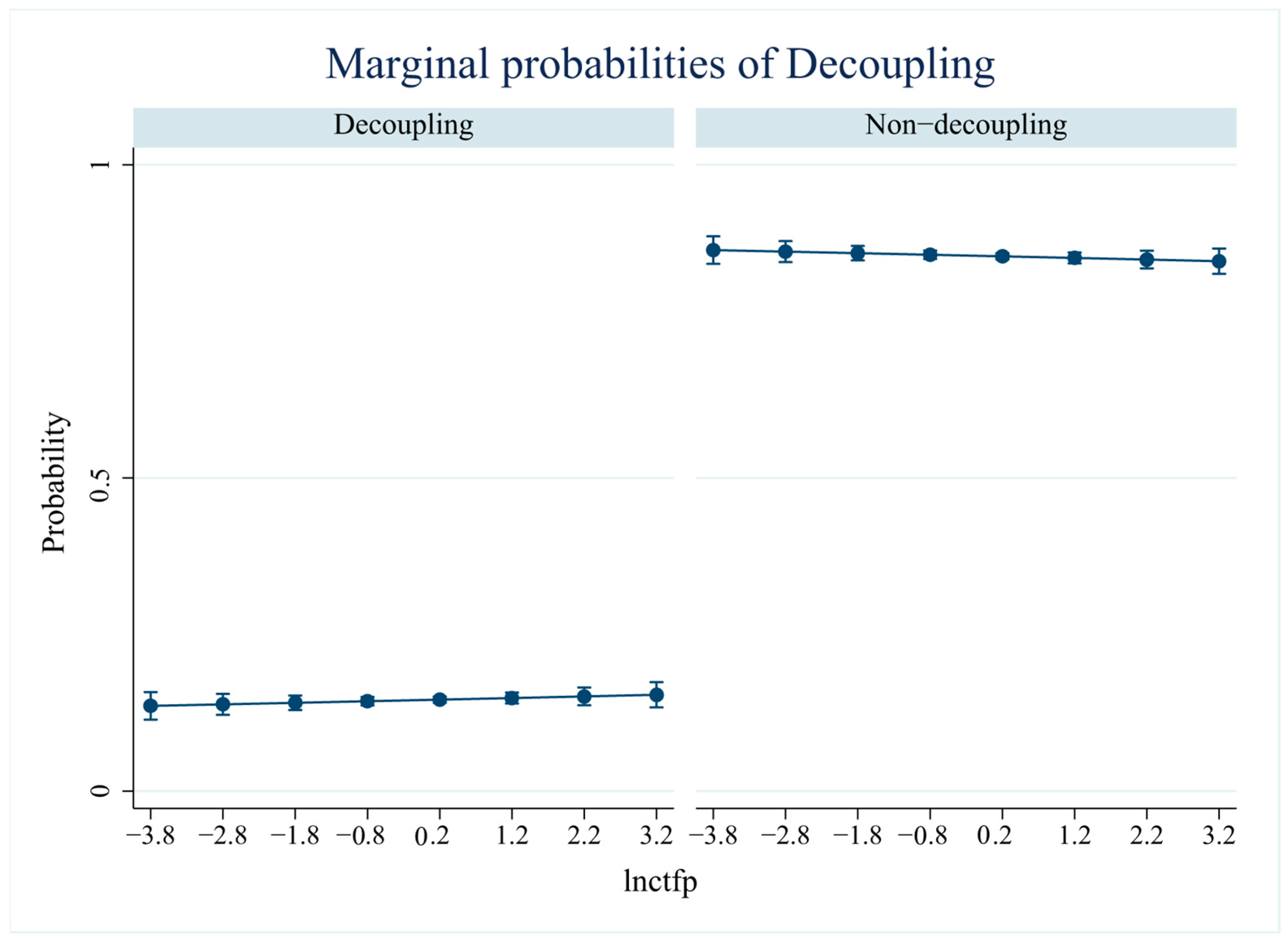
4.3.2. The Different Effects of Emission Reduction Technological Progress Across Counties and Municipal Districts Through the Degree of Decoupling

Following previous studies [5,8], this study employed the production-theoretical decomposition analysis (PDA) approach to measure emission reduction technological progress. The estimation of emission reduction (ln(ctfp)) is based on a distance function, which is presented as follows:

$$D_C^t\left(E^t,Y^t,C^t\right)=sup\left\{{\theta }^t:\left(E^t,Y^t,C^t/{\theta }^t\right)\in S^{t^{\prime }}\right\}$$

(8)

The distance functions for energy consumption and CO₂ emissions are represented by $D_C^t$, which can be assessed through data envelopment analysis (DEA) methods under the constant returns to scale (CRS) assumption. Following the methodology in [5], we formulate the corresponding linear programming problem as follows:

$$\begin{array}{ll}& {\left[D_{C_i}^t\left(E_i^t,Y_i^t,C_i^t\right)\right]}^{-1}=min{\theta }_i^t\\ & s.t.\sum _{i=1}^n{z}_i{E}_i^t\le E_i^t+{\varpi }_i;\\ & \sum _{i=1}^n{z}_i{Y}_i^t\ge Y_i^t;\\ & \sum _{i=1}^n{z}_i{C}_i^t={\theta }_i^t{C}_i^t;z_i\ge 0;{\varpi }_i\ge 0\end{array}$$

(9)

Next, following the method proposed in previous studies [8,21], emission reduction technology can be measured as follows:

$$ctf{p}_i^t={\displaystyle \frac{{\left[D_{C_i}^t\left(E_i^t,Y_i^t,C_i^t\right)\times D_{C_i}^{t+1}\left(E_i^t,Y_i^t,C_i^t\right)\right]}^{1/2}}{{\left[D_{C_i}^t\left(E_i^{t+1},Y_i^{t+1},C_i^{t+1}\right)\times D_{C_i}^{t+1}\left(E_i^{t+1},Y_i^{t+1},C_i^{t+1}\right)\right]}^{1/2}}}$$

(10)

Subsequently, the influence of ln(ctfp) on the quality was indirectly discussed through the decoupling states. Figure 8 shows that the marginal probabilities of decoupling under different emission reduction technology levels. It is evident that county-level regions with better ln(ctfp) may have greater probability of decoupling. However, the slope of the trend is small, implying that emission reduction technological progress has a limited contribution to making CO₂ emissions decoupled from economic growth. Thus, the mechanism through which emission reduction technological progress affects quality by improving the marginal probability of decoupling is not significant.

Subsequently, the effects of emission reduction technology with respect to the quality of the low-carbon economy through the degree of decoupling in counties and municipal districts were explored.

Table 4. Heterogeneous effects of emission reduction technological progress on ln(reo) across counties and municipal districts.

	(1)	(2)
	ln(reo)	ln(reo)
	Counties	Municipal districts
i.tapio#c.ln(ctfp)	0.0245	0.0065 ***
	(0.0222)	(0.0020)
Control variables	Yes	Yes
Individual FE	Yes	Yes
Year FE	Yes	Yes
R2	0.1072	0.1783
N	12,616	3056

Notes: (a) ***, **, and * denote significance at the 1%, 5%, and 1% levels, respectively; and (b) values in parentheses denote robust standard errors.

shows that municipal districts’ ln(ctfp) significantly improved ln(reo) when they achieved the decoupling. Since ln(ctfp) aims at curbing rapid CO₂ emissions growth, it greatly improves municipal districts’ degree of decoupling so as to promote ln(reo). However, the coefficient proved statistically insignificant for counties. These findings suggest that emission reduction technologies contributed more substantially to improving low-carbon economy quality in municipal districts than in counties, whether under strong or weak decoupling conditions. In reality, municipal districts have achieved a high level of economic development, and the enterprises within this region predominantly lead in technological innovation and application across energy efficiency enhancement, renewable energy development, and fossil fuel decarbonization. Consequently, technological advancements in the municipal district have significantly facilitated the decoupling of economic expansion from carbon emissions [29,30,73]. Thus, the different impact of emission reduction technology on the degree of decoupling is a potential reason for the heterogeneous the relationship between neo and reo across counties and municipal districts, consistent with the technological perspective of EKC theory.

To further verify the heterogeneous impacts of emission reduction technology under different types of industrial structure, this study discussed the effects of ln(ctfp) based on different subsamples (i.e., regions with high quartiles of ln(ce), ln(is), and ln(ii)). The regression results are presented in

Table 5. Heterogeneous effects of emission reduction technological progress on ln(reo) across counties and municipal districts with high quartiles of ln(ce), ln(is), and ln(ii).

	(1)	(2)	(3)	(4)	(5)	(6)
	ln(reo)	ln(reo)	ln(reo)	ln(reo)	ln(reo)	ln(reo)
	Counties with high quartiles of ln(ce)	Municipal districts with high quartiles of ln(ce)	Counties with high quartiles of ln(is)	Municipal districts with high quartiles of ln(is)	Counties with high quartiles of ln(ii)	Municipal districts with high quartiles of ln(ii)
i.tapio#c.ln(ctfp)	0.0181	0.0093 ***	0.0255	0.0088 ***	0.0281	0.0035 ***
	(0.0286)	(0.0035)	(0.0178)	(0.0033)	(0.0409)	(0.0013)
Control variables	Yes	Yes	Yes	Yes	Yes	Yes
Individual FE	Yes	Yes	Yes	Yes	Yes	Yes
Year FE	Yes	Yes	Yes	Yes	Yes	Yes
R2	0.3045	0.2968	0.3280	0.2144	0.0885	0.1306
N	3157	1078	2929	1021	5281	1559

Notes: (a) ***, **, and * denote significance at the 1%, 5%, and 1% levels, respectively; and (b) values in parentheses denote robust standard errors.

. Columns (1)–(6) show that ln(ctfp) had more significant effects in municipal districts, especially in regions with high carbon density, high ratio of secondary industry, and high ratio of large-scale industrial output. The results indicate that even if municipal districts have a high proportion of secondary industries (or fossil fuels), their emission reduction technology significantly promotes the degree of decoupling so as to improve the quality. These findings corroborate existing research [5,8].

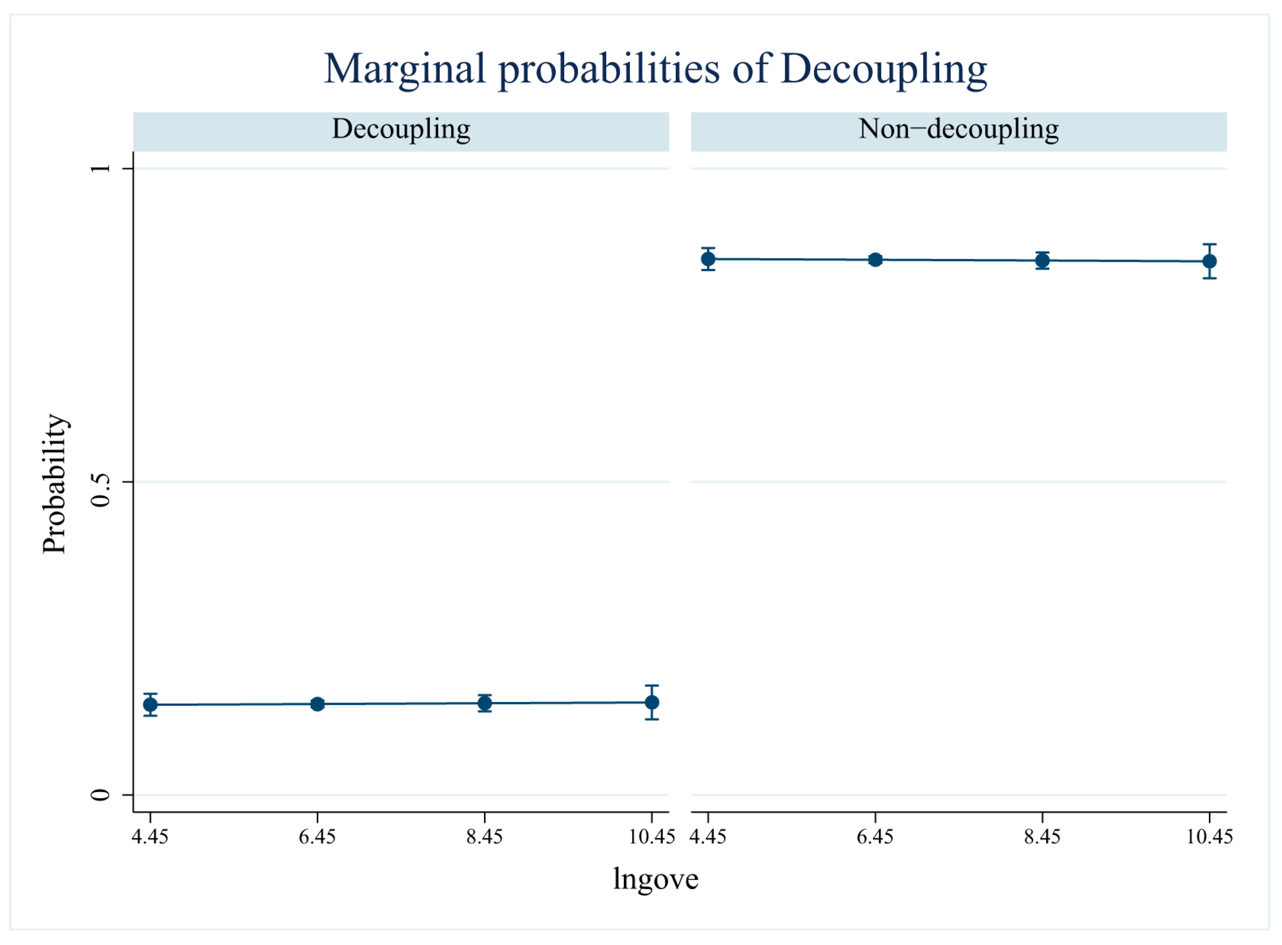
4.3.3. The Different Impacts of Government Intervention Across Counties and Municipal Districts Through the Degree of Decoupling

Following previous studies, the ratio of local general budget expenditure to GDP (ln(gove)) was adopted as an index measuring government intervention in this study [47,48,49]. Figure 9 illustrates how ln(gove) affects the probability of decoupling. The probabilities of decoupling under different government intervention levels failed to change at the 95% confidence interval, indicating that government intervention insignificantly made CO₂ emissions decoupled from economic growth.

Next, the impacts of ln(gove) on counties’ and municipal districts’ ln(reo) in terms of the degree of decoupling were discussed.

Table 6. Heterogeneous effects of government intervention on ln(reo) across counties and municipal districts.

	(1)	(2)
	ln(reo)	ln(reo)
	Counties	Municipal districts
i.tapio#c.ln(gove)	0.0025	0.0106 ***
	(0.0015)	(0.0030)
Control variables	Yes	Yes
Individual FE	Yes	Yes
Year FE	Yes	Yes
R2	0.1094	0.1808
N	12,616	3056

Notes: (a) ***, **, and * denote significance at the 1%, 5%, and 1% levels, respectively; and (b) values in parentheses denote robust standard errors.

reports that the coefficient was only significant in municipal districts rather than counties. The results imply that the different impacts of government intervention on the degree of decoupling were responsible for the heterogeneous impacts of neo growth on reo growth across counties and municipal districts.

Further, subsamples based on the upper quartiles of ln(ce), ln(is), and ln(ii) were chosen to make regressions.

Table 7. Heterogeneous effects of government intervention on ln(reo) across counties and municipal districts with high quartiles of ln(ce), ln(is) and ln(ii).

	(1)	(2)	(3)	(4)	(5)	(6)
	ln(reo)	ln(reo)	ln(reo)	ln(reo)	ln(reo)	ln(reo)
	Counties with high quartiles of ln(ce)	Municipal districts with high quartiles of ln(ce)	Counties with high quartiles of ln(is)	Municipal districts with high quartiles of ln(is)	Counties with high quartiles of ln(ii)	Municipal districts with high quartiles of ln(ii)
i.tapio#c.ln(gove)	0.0024 **	0.0178 ***	0.0007	0.0122 ***	0.0016 **	0.0069 ***
	(0.0011)	(0.0064)	(0.0005)	(0.0038)	(0.0007)	(0.0019)
Control variables	Yes	Yes	Yes	Yes	Yes	Yes
Individual FE	Yes	Yes	Yes	Yes	Yes	Yes
Year FE	Yes	Yes	Yes	Yes	Yes	Yes
R2	0.3045	0.2968	0.3280	0.2144	0.0885	0.1306
N	3157	1078	2929	1021	5281	1559

Notes: (a) ***, **, and * denote significance at the 1%, 5%, and 1% levels, respectively; and (b) values in parentheses denote robust standard errors.

presents that both counties’ and municipal districts’ ln(gove) had significant and positive effects on ln(reo) when their ln(ce) and ln(ii) reached seriously high levels. In particular, the 95% confidence interval coefficients in counties and municipal districts based on the subsample with a high quartile of ln(ce) were (+0.00025, +0.0045) and (+0.0051, +0.0304), respectively. Similarly, the 95% confidence interval coefficients in counties and municipal districts based on the subsample with a high quartile of ln(ii) were (+0.00028, +0.0029) and (+0.00304, +0.011), respectively.

With regard to the subsample with a high quartile of ln(is), the coefficient was only significant in municipal districts. In summary, although local government intervention significantly promoted counties’ and municipal districts’ quality of the low-carbon economy via the decoupling channel, the positive influence was greater in municipal districts. The results further confirmed that local government intervention was a significant channel for causing the heterogeneous relationship between neo and reo across counties and municipal districts.

5. Conclusions and Policy Implications

We investigated the heterogeneous relationship between scale and quality, as well as its potential causes. We observed the following: (1) County-level quality growth had a statistically significant positive impact on scale growth, indicating that China’s current low-carbon development strategy to improve quality is timely and will not threaten scale growth in the long term. (2) However, quantity growth in counties (especially those with substantial fossil fuel energy consumption and secondary industry’s output) negatively influenced quality growth, while it had an insignificant effect in municipal districts. This heterogeneity confirmed that counties and municipal districts are at different stages of the Environmental Kuznets Curve. (3) In particular, secondary industry development, large-scale industrial output intensity, and a resource-based mode were responsible for the heterogeneous the relationship between scale and quality. (4) Moreover, although emission reduction technological progress and local government intervention failed to significantly change the marginal probability of decoupling between economic growth and CO₂ emissions, they played a greater role in improving the quality of municipal districts than that of counties, as evidenced by the degree of decoupling.

Based on empirical findings, we propose several policy implications:

(1)

To mitigate the negative impact of scale expansion on quality growth, counties—particularly those with secondary industry dominance and resource-dependent development models—must prioritize transforming their economic growth patterns. This transformation should emphasize industrial structure optimization and energy consumption restructuring to achieve effective decoupling. Key strategies for transitioning toward low-carbon development include systematically phasing out obsolete production capacities and energy-intensive equipment, with particular attention paid to reducing disproportionate secondary industry representation. Governments should implement tiered subsidy mechanisms that progressively reward enterprises adopting clean production technologies, complemented by fiscal incentives such as income tax reductions for renewable energy investments. Concurrently, county authorities need to establish differentiated emission control systems, mandating regular energy efficiency audits and operational permit renewals for high-carbon emitters, while intensifying oversight of critical sectors. Ecologically vulnerable areas require prioritized comprehensive restoration initiatives that strategically allocate land resources through measures like eco-agricultural conversion to enhance carbon sequestration capacity. Pilot low-carbon demonstration zones integrating smart energy management systems and real-time emission monitoring platforms should be developed to synergistically optimize economic development and ecological sustainability.

(2)

Enhancing the decoupling between economic growth and CO₂ emissions necessitates coordinated advancement of emission-reduction technologies and robust governmental intervention. Counties should bridge the maturity gap with urban districts by increasing R&D investment in environmental technologies and strengthening regulatory stringency. Targeted measures should include implementing government-subsidized carbon capture and storage demonstration projects, particularly in high carbon-density industrial zones and depleted hydrocarbon fields suitable for geological storage. Concurrently, counties with subnational forest coverage averages must prioritize afforestation and vegetation restoration programs, focusing on degraded woodland rehabilitation to amplify carbon sink functionality. These integrated approaches—combining industrial modernization, technological innovation, and ecological protection—establish a self-reinforcing mechanism that progressively dissociates economic expansion from carbon emissions while enhancing regional development sustainability.

References

1. Tang, Z.; Shi, C.B.; Liu, Z. Sustainable development of tourism industry in China under the low-carbon economy. Energy Procedia 2011, 5, 1303–1307. [Google Scholar] [CrossRef]
2. Bridge, G.; Bouzarovski, S.; Bradshaw, M.; Eyre, N. Geographies of energy transition: Space, place and the low-carbon economy. Energy Policy 2013, 53, 331–340. [Google Scholar] [CrossRef]
3. Cai, X.; Lu, Y.; Wu, M.; Yu, L. Does environmental regulation drive away inbound foreign direct investment? Evidence from a quasi-natural experiment in China. J. Dev. Econ. 2016, 123, 73–85. [Google Scholar] [CrossRef]
4. Lyu, P.H.; Ngai, E.W.; Wu, P.Y. Scientific data-driven evaluation on academic articles of low-carbon economy. Energy Policy 2019, 125, 358–367. [Google Scholar] [CrossRef]
5. Chen, J.; Gao, M.; Cheng, S.; Xu, Y.; Song, M.; Liu, Y.; Hou, W.; Wang, S. Evaluation and drivers of global low-carbon economies based on satellite data. Humanit. Soc. Sci. Commun. 2022, 9, 153. [Google Scholar] [CrossRef]
6. Shahbaz, M.; Ozturk, I.; Afza, T.; Ali, A. Revisiting the environmental Kuznets curve in a global economy. Renew. Sustain. Energy Rev. 2013, 25, 494–502. [Google Scholar] [CrossRef]
7. Schmidt, T.S. Low-carbon investment risks and de-risking. Nat. Clim. Change 2014, 44, 237–239. [Google Scholar] [CrossRef]
8. Gao, M. The impacts of carbon trading policy on China’s low-carbon economy based on county-level perspectives. Energy Policy 2023, 175, 113494. [Google Scholar] [CrossRef]
9. Talberth, J.; Bohara, A.K. Economic openness and green GDP. Ecol. Econ. 2006, 58, 743–758. [Google Scholar] [CrossRef]
10. Van den Bergh, J.C.; Botzen, W.J.W. Monetary valuation of the social cost of CO2 emissions: A critical survey. Ecol. Econ. 2015, 114, 33–46. [Google Scholar] [CrossRef]
11. Vaghefi, N.; Siwar, C.; Aziz, S.A.A.G. Green GDP and sustainable development in Malaysia. Curr. World Environ. 2015, 101, 1. [Google Scholar] [CrossRef]
12. Kunanuntakij, K.; Varabuntoonvit, V.; Vorayos, N.; Panjapornpon, C.; Mungcharoen, T. Thailand Green GDP assessment based on environmentally extended input-output model. J. Clean. Prod. 2017, 167, 970–977. [Google Scholar] [CrossRef]
13. Stjepanović, S.; Tomić, D.; Škare, M. A new approach to measuring green GDP: A cross-country analysis. Entrep. Sustain. Issues 2017, 4, 574. [Google Scholar] [CrossRef] [PubMed]
14. Yang, C.; Poon, J.P. Regional Analysis of China’s Green GDP. Eurasian Geogr. Econ. 2009, 50, 547–563. [Google Scholar] [CrossRef]
15. Zimmer, A.; Jakob, M.; Steckel, J.C. What motivates Vietnam to strive for a low-carbon economy?-On the drivers of climate policy in a developing country. Energy Sustain. Dev. 2015, 24, 19–32. [Google Scholar] [CrossRef]
16. Zhang, Y.; Shen, L.; Shuai, C.; Tan, Y.; Ren, Y.; Wu, Y. Is the low-carbon economy efficient in terms of sustainable development? A global perspective. Sustain. Dev. 2019, 27, 130–152. [Google Scholar] [CrossRef]
17. Liu, Y.; Wang, M.; Feng, C. Inequalities of China’s regional low-carbon development. J. Environ. Manag. 2020, 274, 111042. [Google Scholar] [CrossRef]
18. Wu, S.; Han, H. Sectoral changing patterns of China’s green GDP considering climate change: An investigation based on the economic input-output life cycle assessment model. J. Clean. Prod. 2020, 251, 119764. [Google Scholar] [CrossRef]
19. Zheng, J.; Shao, X.; Liu, W.; Kong, J.; Zuo, G. The impact of the pilot program on industrial structure upgrading in low-carbon cities. J. Clean. Prod. 2021, 290, 125868. [Google Scholar] [CrossRef]
20. Grossman, G.M.; Krueger, A.B. Economic growth and the environment. Q. J. Econ. 1995, 1102, 353–377. [Google Scholar] [CrossRef]
21. Chen, J.; Xu, C.; Cui, L.; Huang, S.; Song, M. Driving factors of CO2 emissions and inequality characteristics in China: A combined decomposition approach. Energy Econ. 2019, 78, 589–597. [Google Scholar] [CrossRef]
22. Shan, Y.; Fang, S.; Cai, B.; Zhou, Y.; Li, D.; Feng, K.; Hubacek, K. Chinese cities exhibit varying degrees of decoupling of economic growth and CO2 emissions between 2005 and 2015. One Earth 2021, 41, 124–134. [Google Scholar] [CrossRef]
23. Shang, L.; Xu, P. Can Carbon Emission Regulation Achieve a Dual Target of Low Carbon and Employment? An Empirical Analysis Based on China’s Provincial Panel Data. Front. Energy Res. 2022, 10, 926443. [Google Scholar] [CrossRef]
24. Campiglio, E. Beyond carbon pricing: The role of banking and monetary policy in financing the transition to a low-carbon economy. Ecol. Econ. 2016, 121, 220–230. [Google Scholar] [CrossRef]
25. Wu, Y.; Zhu, Q.; Zhu, B. Comparisons of decoupling trends of global economic growth and energy consumption between developed and developing countries. Energy Policy 2018, 116, 30–38. [Google Scholar] [CrossRef]
26. Mardani, A.; Streimikiene, D.; Cavallaro, F.; Loganathan, N.; Khoshnoudi, M. Carbon dioxide CO2 emissions and economic growth: A systematic review of two decades of research from 1995 to 2017. Sci. Total Environ. 2019, 649, 31–49. [Google Scholar] [CrossRef]
27. Li, G.; Wei, W. Financial development, openness, innovation, carbon emissions, and economic growth in China. Energy Econ. 2021, 97, 105194. [Google Scholar] [CrossRef]
28. Sharif, F.; Tauqir, A. The effects of infrastructure development and carbon emissions on economic growth. Environ. Sci. Pollut. Res. 2021, 28, 36259–36273. [Google Scholar] [CrossRef] [PubMed]
29. Lu, Q.; Yang, H.; Huang, X.; Chuai, X.; Wu, C. Multi-sectoral decomposition in decoupling industrial growth from carbon emissions in the developed Jiangsu Province, China. Energy 2015, 82, 414–425. [Google Scholar] [CrossRef]
30. Hang, Y.; Wang, Q.; Zhou, D.; Zhang, L. Factors influencing the progress in decoupling economic growth from carbon dioxide emissions in China’s manufacturing industry. Resour. Conserv. Recycl. 2019, 146, 77–88. [Google Scholar] [CrossRef]
31. Zhang, Z. Asian energy and environmental policy: Promoting growth while preserving the environment. Energy Policy 2008, 3610, 3905–3924. [Google Scholar] [CrossRef]
32. Hu, Y.; Liu, J.; Ahmed, M. Does emission trading policy restrain economy? A county-scale empirical assessment from Zhejiang Province of China. Energy Policy 2022, 168, 113138. [Google Scholar] [CrossRef]
33. Ziaei, S.M. Effects of financial development indicators on energy consumption and CO2 emission of European, East Asian and Oceania countries. Renew. Sustain. Energy Rev. 2015, 42, 752–759. [Google Scholar] [CrossRef]
34. Adams, S.; Klobodu, E.K.M.; Opoku, E.E.O. Energy consumption, political regime and economic growth in sub-Saharan Africa. Energy Policy 2016, 96, 36–44. [Google Scholar] [CrossRef]
35. Antonakakis, N.; Chatziantoniou, I.; Filis, G. Energy consumption, CO2 emissions, and economic growth: An ethical dilemma. Renew. Sustain. Energy Rev. 2017, 68, 808–824. [Google Scholar] [CrossRef]
36. Pan, W.; Pan, W.; Hu, C.; Tu, H.; Zhao, C.; Yu, D.; Xiong, J.; Zheng, G. Assessing the green economy in China: An improved framework. J. Clean. Prod. 2019, 209, 680–691. [Google Scholar] [CrossRef]
37. Al-Mulali, U. Investigating the impact of nuclear energy consumption on GDP growth and CO2 emission: A panel data analysis. Prog. Nucl. Energy 2014, 73, 172–178. [Google Scholar] [CrossRef]
38. Rajbhandari, A.; Zhang, F. Does energy efficiency promote economic growth? Evidence from a multicountry and multisectoral panel dataset. Energy Econ. 2018, 69, 128–139. [Google Scholar] [CrossRef]
39. Chen, J.; Liu, J.; Qi, J.; Gao, M.; Cheng, S.; Li, K.; Xu, C. City- county-level spatio-temporal energy consumption and efficiency datasets for China from 1997 to 2017. Sci. Data 2022, 91, 101. [Google Scholar] [CrossRef]
40. Cheng, Z.; Li, L.; Liu, J. Industrial structure, technical progress and carbon intensity in China’s provinces. Renew. Sustain. Energy Rev. 2018, 81, 2935–2946. [Google Scholar] [CrossRef]
41. Huang, J.; Liu, Q.; Cai, X.; Hao, Y.; Lei, H. The effect of technological factors on China’s carbon intensity: New evidence from a panel threshold model. Energy Policy 2018, 115, 32–42. [Google Scholar] [CrossRef]
42. Tapio, P. Towards a theory of decoupling: Degrees of decoupling in the EU and the case of road traffic in Finland between 1970 and 2001. Transp. Policy 2005, 122, 137–151. [Google Scholar] [CrossRef]
43. Coderoni, S.; Esposti, R. CAP payments and agricultural GHG emissions in Italy. A farm-level assessment. Sci. Total Environ. 2018, 627, 427–437. [Google Scholar] [CrossRef]
44. Srivastava, A.; Van Passel, S.; Kessels, R.; Valkering, P.; Laes, E. Reducing winter peaks in electricity consumption: A choice experiment to structure demand response programs. Energy Policy 2020, 137, 111183. [Google Scholar] [CrossRef]
45. Yang, M.; Wang, E.Z.; Hou, Y. The relationship between manufacturing growth and CO2 emissions: Does renewable energy consumption matter? Energy 2021, 232, 121032. [Google Scholar] [CrossRef]
46. Liu, F.; Kang, Y.; Guo, K. Is electricity consumption of Chinese counties decoupled from carbon emissions? A study based on Tapio decoupling index. Energy 2022, 251, 123879. [Google Scholar] [CrossRef]
47. Pan, X.; Li, M.; Guo, S.; Pu, C. Research on the competitive effect of local government’s environmental expenditure in China. Sci. Total Environ. 2020, 718, 137238. [Google Scholar] [CrossRef] [PubMed]
48. Kou, J.; Xu, X. Does internet infrastructure improve or reduce carbon emission performance?--A dual perspective based on local government intervention and market segmentation. J. Clean. Prod. 2022, 379, 134789. [Google Scholar] [CrossRef]
49. Yan, Y.; Huang, J. The role of population agglomeration played in China’s carbon intensity: A city-level analysis. Energy Econ. 2022, 114, 106276. [Google Scholar] [CrossRef]
50. Pollitt, M.G. A global carbon market? Front. Eng. Manag. 2019, 6, 5–18. [Google Scholar] [CrossRef]
51. Chen, X.; Nordhaus, W.D. Using luminosity data as a proxy for economic statistics. Proc. Natl. Acad. Sci. USA 2011, 108, 8589–8594. [Google Scholar] [CrossRef] [PubMed]
52. Henderson, J.; Vernon, A.S.; Weil, D.N. Measuring economic growth from outer space. Am. Econ. Rev. 2012, 102, 994–1028. [Google Scholar] [CrossRef] [PubMed]
53. Hu, Y.; Yao, J. Illuminating economic growth. J. Econ. 2021, 228, 359–378. [Google Scholar] [CrossRef]
54. Dong, F.; Dai, Y.; Zhang, S.; Zhang, X.; Long, R. Can a carbon emission trading scheme generate the Porter effect? Evidence from pilot areas in China. Sci. Total Environ. 2019, 653, 565–577. [Google Scholar] [CrossRef] [PubMed]
55. Cheng, S.; Fan, W.; Meng, F.; Chen, J.; Liang, S.; Song, M.; Liu, G.; Casazza, M. Potential role of fiscal decentralization on interprovincial differences in CO2 emissions in China. Environ. Sci. Technol. 2020, 55, 813–822. [Google Scholar] [CrossRef]
56. Jones, M.W.; Andrew, R.M.; Peters, G.P.; Janssens-Maenhout, G.; De-Gol, A.J.; Ciais, P.; Patra, P.K.; Chevallier, F.; Le Quéré, C. Gridded fossil CO2 emissions and related O2 combustion consistent with national inventories 1959–2018. Sci. Data 2021, 8, 2. [Google Scholar] [CrossRef]
57. Harris, N.L.; Gibbs, D.A.; Baccini, A.; Birdsey, R.A.; de Bruin, S.; Farina, M.; Fatoyinbo, L.; Hansen, M.C.; Herold, M.; Houghton, R.A.; et al. Global maps of twenty-first century forest carbon fluxes. Nat. Clim. Change 2021, 11, 234–240. [Google Scholar] [CrossRef]
58. Lv, Q.; Liu, H.; Wang, J.; Liu, H.; Shang, Y. Multiscale analysis on spatiotemporal dynamics of energy consumption CO2 emissions in China: Utilizing the integrated of DMSP-OLS and NPP-VIIRS nighttime light datasets. Sci. Total Environ. 2020, 703, 134394. [Google Scholar] [CrossRef]
59. Chen, J.; Gao, M.; Cheng, S.; Hou, W.; Song, M.; Liu, X.; Liu, Y. Global 1 km × 1 km gridded revised real gross domestic product and electricity consumption during 1992–2019 based on calibrated nighttime light data. Sci. Data 2022, 9, 202. [Google Scholar] [CrossRef]
60. Cai, S.; Liu, D.; Sulla-Menashe, D.; Friedl, M.A. Enhancing MODIS land cover product with a spatial–temporal modeling algorithm. Remote Sens. Environ. 2014, 147, 243–255. [Google Scholar] [CrossRef]
61. He, S.; Li, J.; Wang, J.; Liu, F. Evaluation and analysis of upscaling of different land use/land cover products FORM-GLC30, GLC_FCS30, CCI_LC, MCD12Q1 and CNLUCC: A case study in China. Geocarto Int. 2022, 37, 17340–17360. [Google Scholar] [CrossRef]
62. Zhao, M.; Running, S.W. Drought-induced reduction in global terrestrial net primary production from 2000 through 2009. Science 2010, 3295994, 940–943. [Google Scholar] [CrossRef] [PubMed]
63. Choi, I. Unit root tests for panel data. J. Int. Money Fin. 2001, 20, 249–272. [Google Scholar] [CrossRef]
64. Dinda, S. Environmental Kuznets curve hypothesis: A survey. Ecol. Econ. 2004, 494, 431–455. [Google Scholar] [CrossRef]
65. Dinda, S. A theoretical basis for the environmental Kuznets curve. Ecol. Econ. 2005, 533, 403–413. [Google Scholar] [CrossRef]
66. Gu, W.; Zhao, X.; Yan, X.; Wang, C.; Li, Q. Energy technological progress, energy consumption, and CO2 emissions: Empirical evidence from China. J. Clean. Prod. 2019, 236, 117666. [Google Scholar] [CrossRef]
67. Li, D.; Gao, M.; Hou, W.; Song, M.; Chen, J. A modified and improved method to measure economy-wide carbon rebound effects based on the PDA-MMI approach. Energy Policy 2020, 147, 111862. [Google Scholar] [CrossRef]
68. Meng, Y.; Liu, L.; Wang, J.; Ran, Q.; Yang, X.; Shen, J. Assessing the impact of the national sustainable development planning of resource-based cities policy on pollution emission intensity: Evidence from 270 prefecture-level cities in China. Sustainability 2021, 1313, 7293. [Google Scholar] [CrossRef]
69. Yu, C.; Li, H.; Jia, X.; Li, Q. Improving resource utilization efficiency in China’s mineral resource-based cities: A case study of Chengde, Hebei province. Resour. Conserv. Recycl. 2015, 94, 1–10. [Google Scholar] [CrossRef]
70. Yu, B.; Fang, D.; Kleit, A.N.; Xiao, K. Exploring the driving mechanism and the evolution of the low-carbon economy transition: Lessons from OECD developed countries. World Econ. 2022, 45, 2766–2795. [Google Scholar] [CrossRef]
71. Zhang, F.; Deng, X.; Phillips, F.; Fang, C.; Wang, C. Impacts of industrial structure and technical progress on carbon emission intensity: Evidence from 281 cities in China. Technol. Forecast. Soc. Change 2020, 154, 119949. [Google Scholar] [CrossRef]
72. Li, X.; Li, C.; Guo, X. Environmental practices, family control, and corporate performance: Evidence from Chinese family firms. Emerg. Mark. Rev. 2022, 55, 100953. [Google Scholar] [CrossRef]
73. Pan, X.; Guo, S.; Xu, H.; Tian, M.; Pan, X.; Chu, J. China’s carbon intensity factor decomposition and carbon emission decoupling analysis. Energy 2022, 239, 122175. [Google Scholar] [CrossRef]
Figure 1. The research roadmap.
Sustainability 17 03572 g001
Figure 2. Cumulative generalized impulse responses of neo growth, reo growth, and e growth based on orthogonalization: (a) counties and (b) municipal districts.
Sustainability 17 03572 g002
Figure 3. Cumulative generalized impulse responses of counties’ neo growth, reo growth, and e growth based on subsample analysis. (a) Subsample was chosen based on low quartile of carbon density. (b) Subsample was chosen based on high quartile of carbon density.
Sustainability 17 03572 g003
Figure 4. Cumulative generalized impulse responses of counties’ neo growth, reo growth, and e growth based on subsample analysis. (a) Subsample was chosen based on low quartile of the ratio of secondary industry’s output. (b) Subsample was chosen based on high quartile of the ratio of secondary industry’s output.
Sustainability 17 03572 g004
Figure 5. Cumulative generalized impulse responses of counties’ neo (low-carbon GDP) growth, reo (ratio of neo to GDP) growth, and e (energy consumption) growth based on subsample analysis. (a) Counties in key cities for environmental protection. (b) Counties in non-key cities for environmental protection.
Sustainability 17 03572 g005
Figure 6. Cumulative generalized impulse responses of counties’ y (GDP) growth, ci (carbon intensity) growth, and e (energy consumption) growth based on subsample analysis: (a) counties and (b) municipal districts.
Sustainability 17 03572 g006
Figure 7. Cumulative generalized impulse responses of counties’ neo growth, reo growth, e growth, and u growth based on subsample analysis. (a) Counties with high quartile of carbon density. (b) Counties with high quartile of the ratio of secondary industry’s output.
Sustainability 17 03572 g007
Figure 8. The changes in marginal probabilities of decoupling under different emission reduction technology levels.
Sustainability 17 03572 g008
Figure 9. The changes in marginal probabilities of decoupling under different government intervention levels.
Sustainability 17 03572 g009