
Convolutional Neural Network Models in Municipal Solid Waste Classification: Towards Sustainable Management

 , ,
, ,  , and
, and
Abstract
1. Introduction
Literature Review
2. Materials and Methods
2.1. Materials
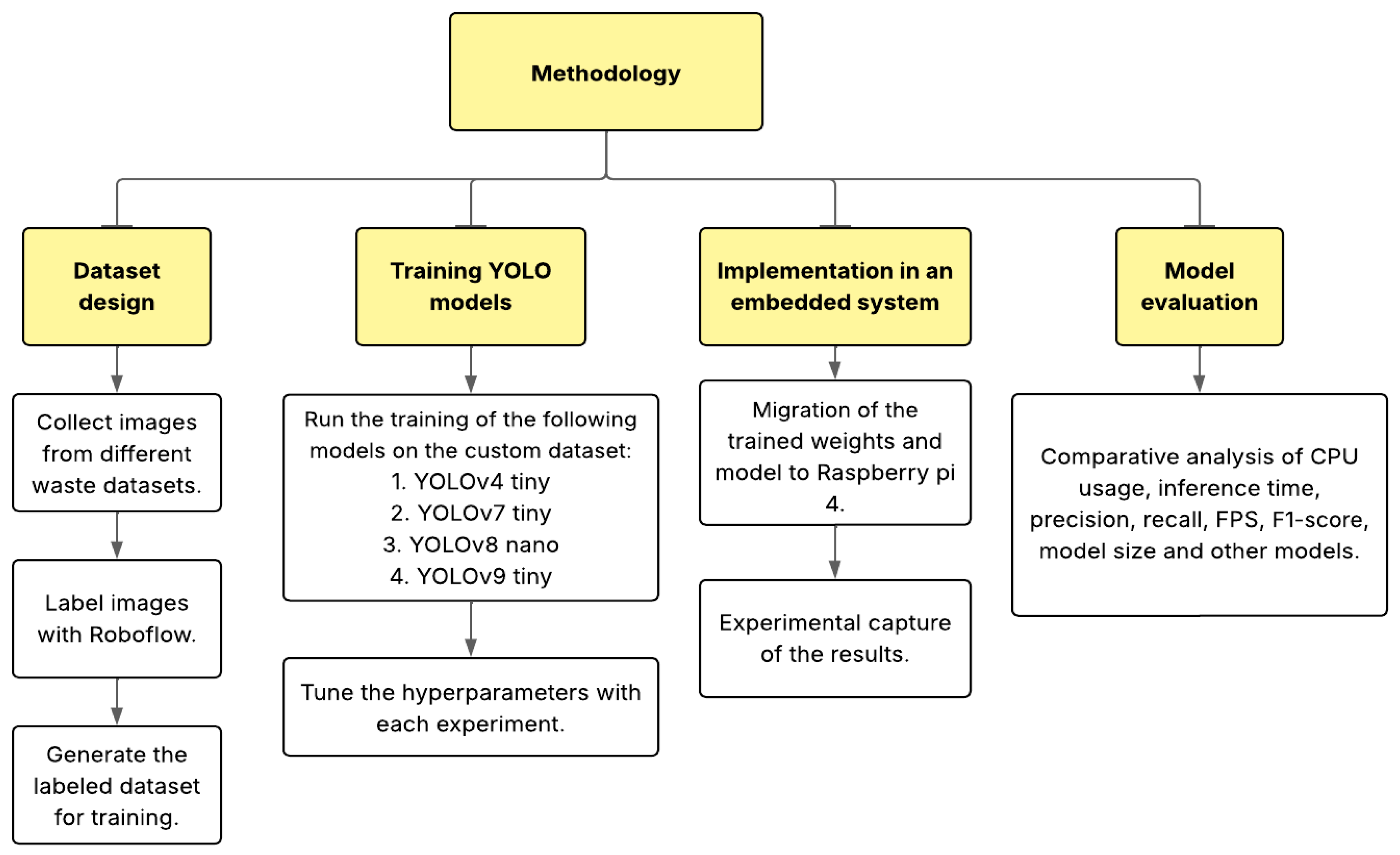
2.2. Methodology
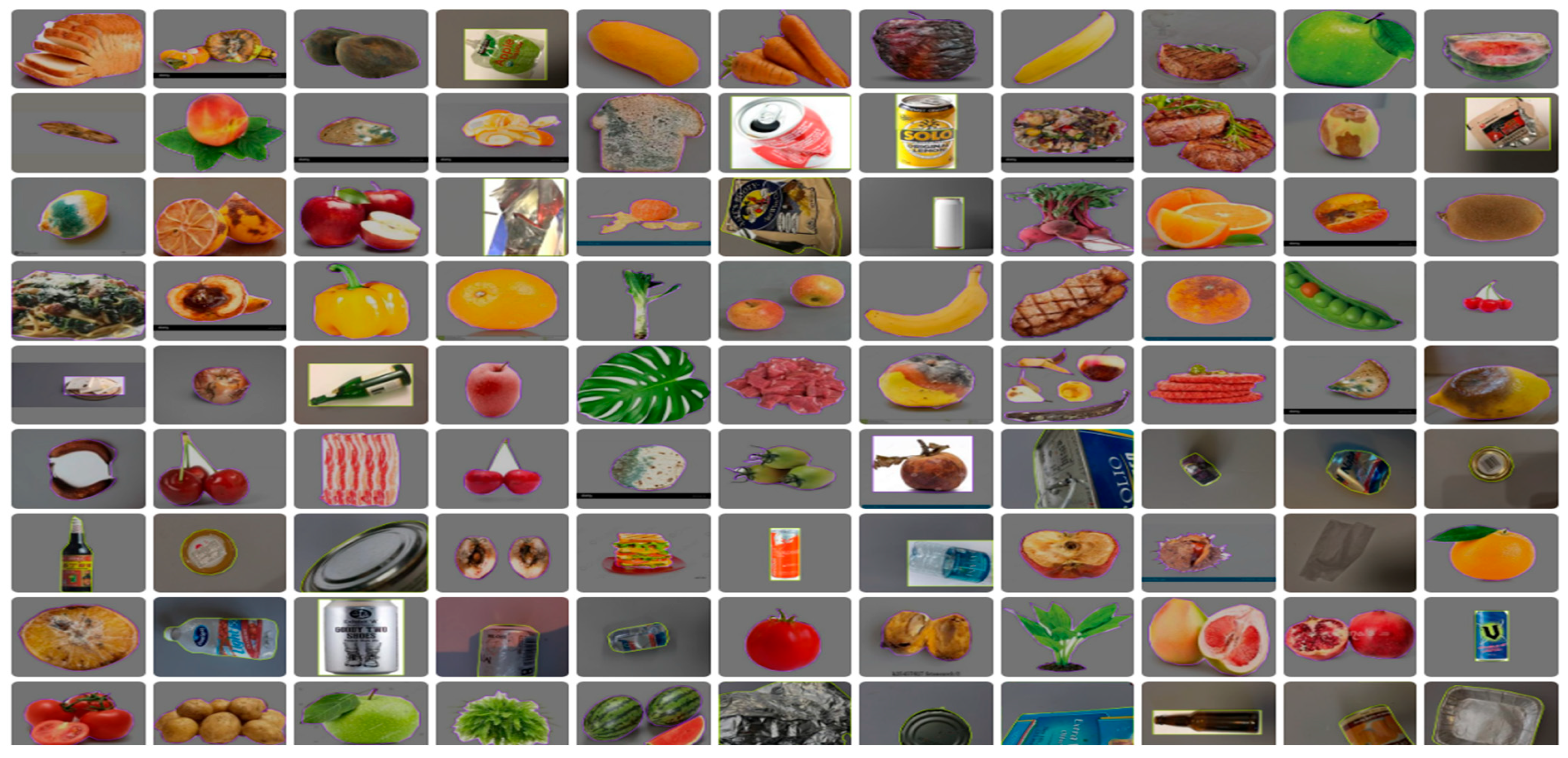
2.2.1. Dataset Design
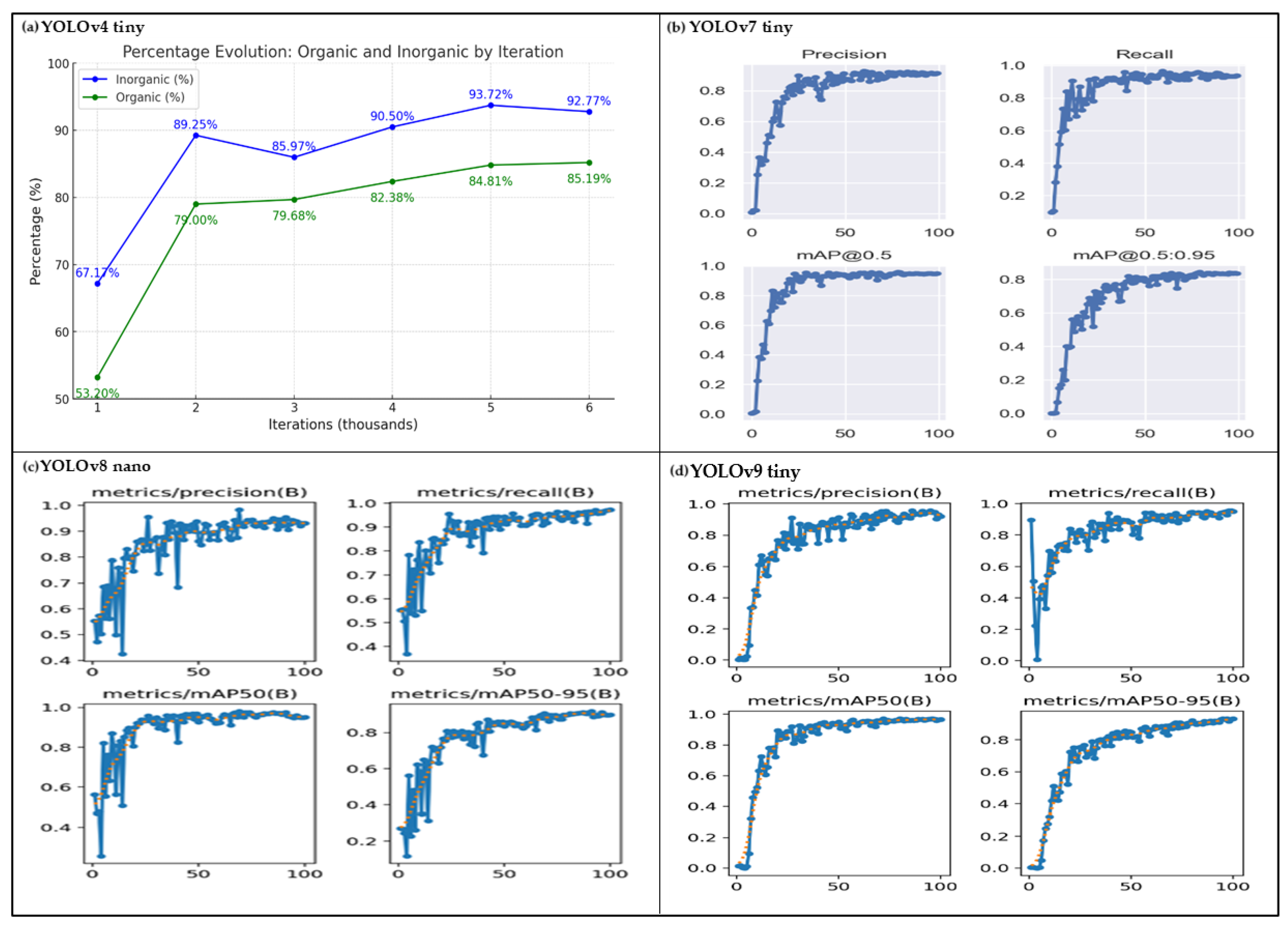
2.2.2. YOLO Model Training
Validation Metrics
- The Intersection over Union (IoU)
- Precision
- Recall
- F1-score
2.2.3. Embedded System Implementation
Energy Usage Methods
2.2.4. Model Evaluation
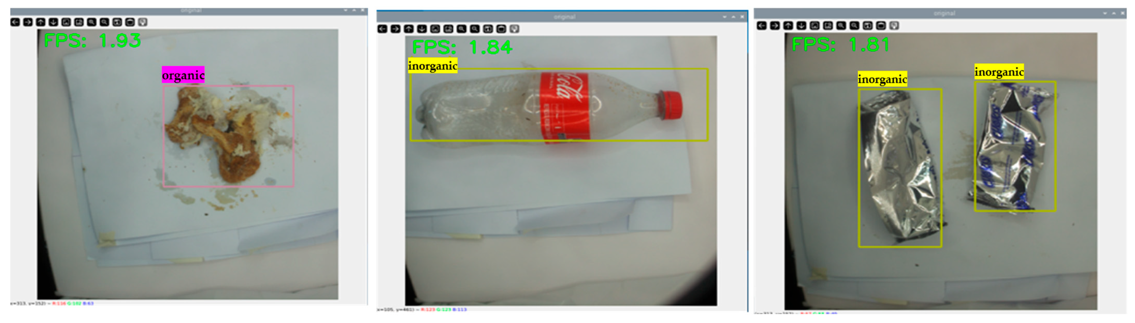
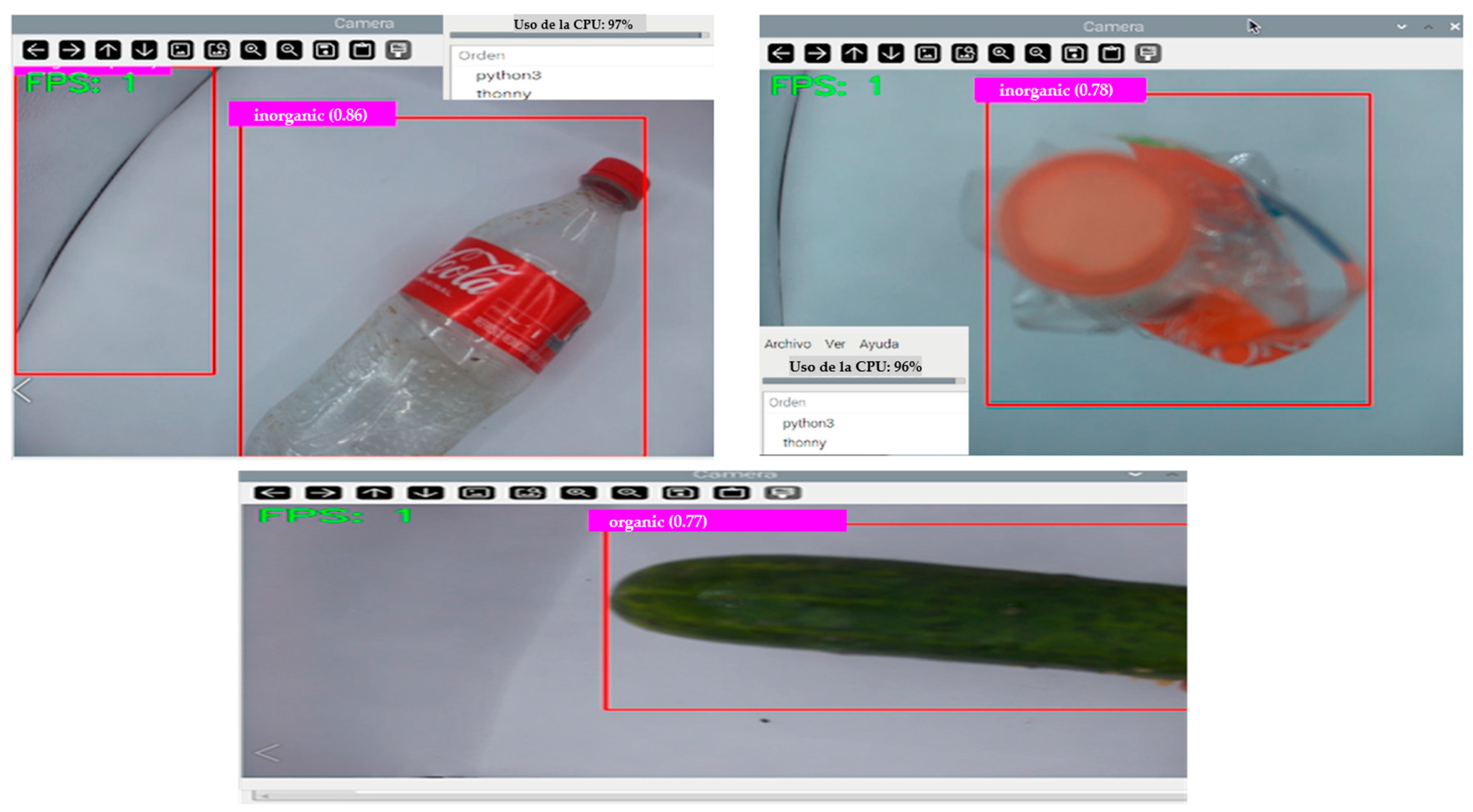
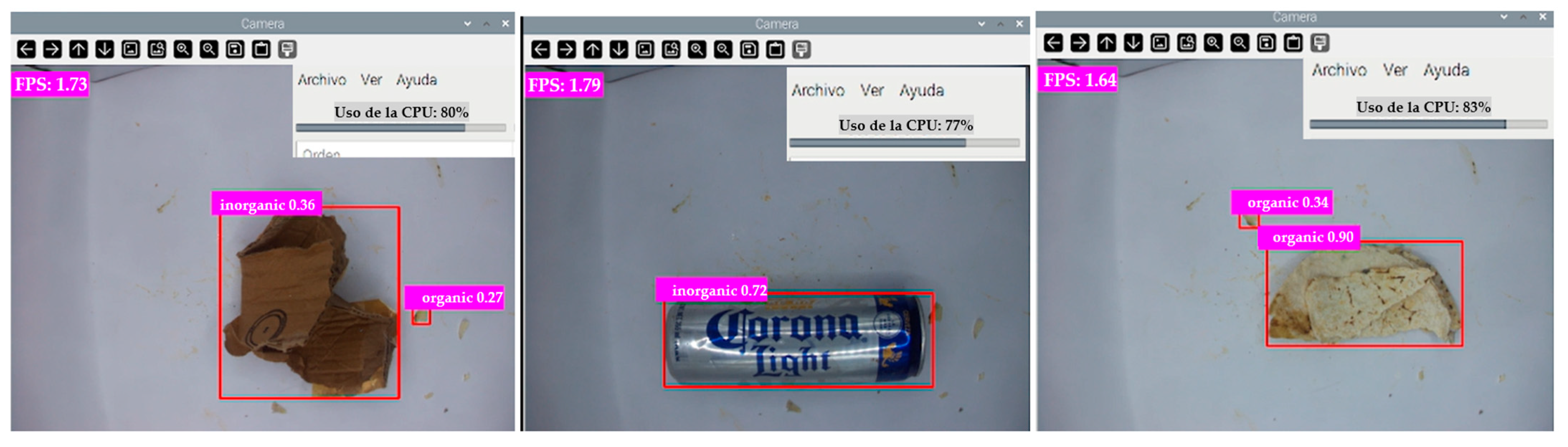
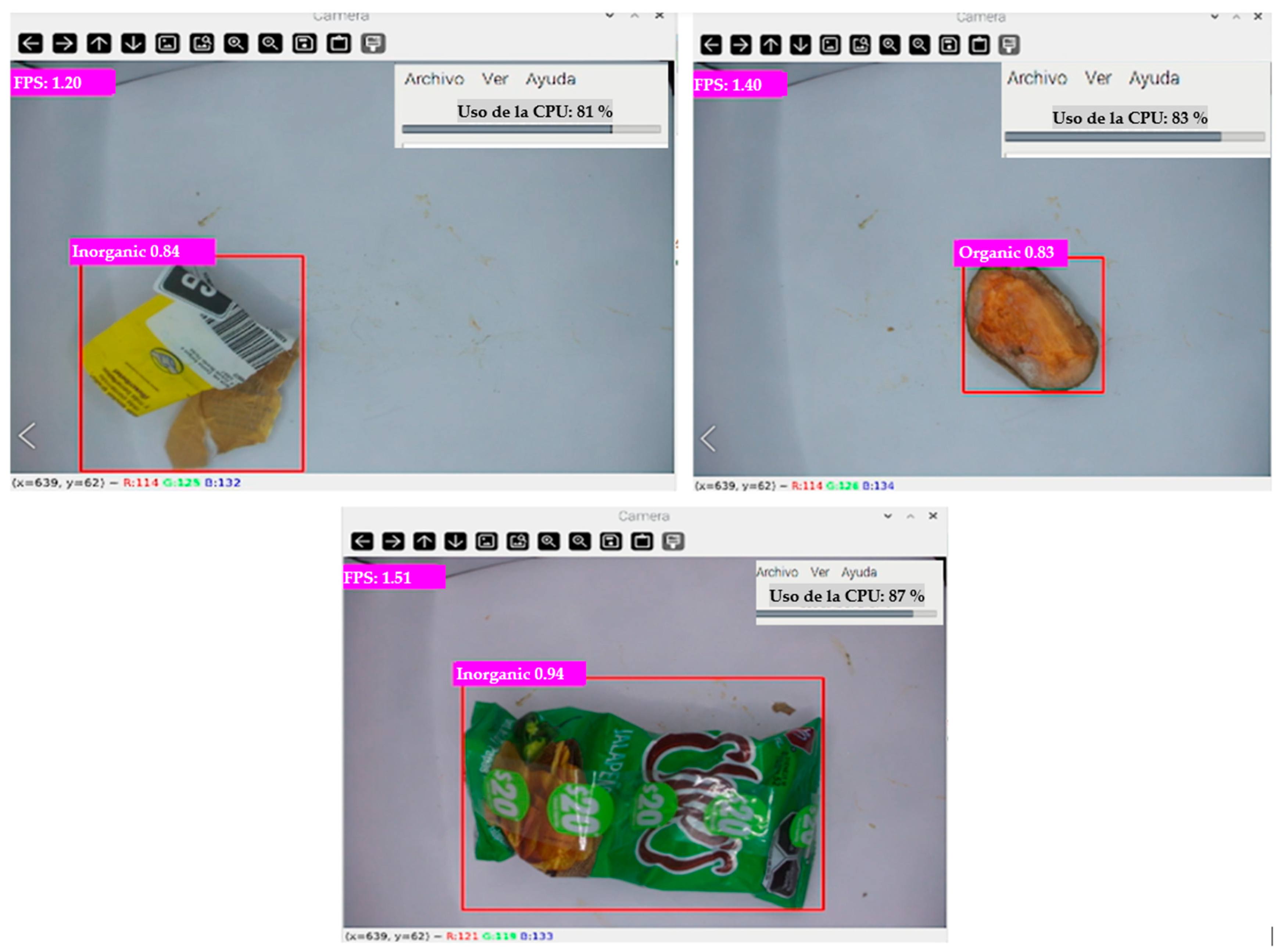
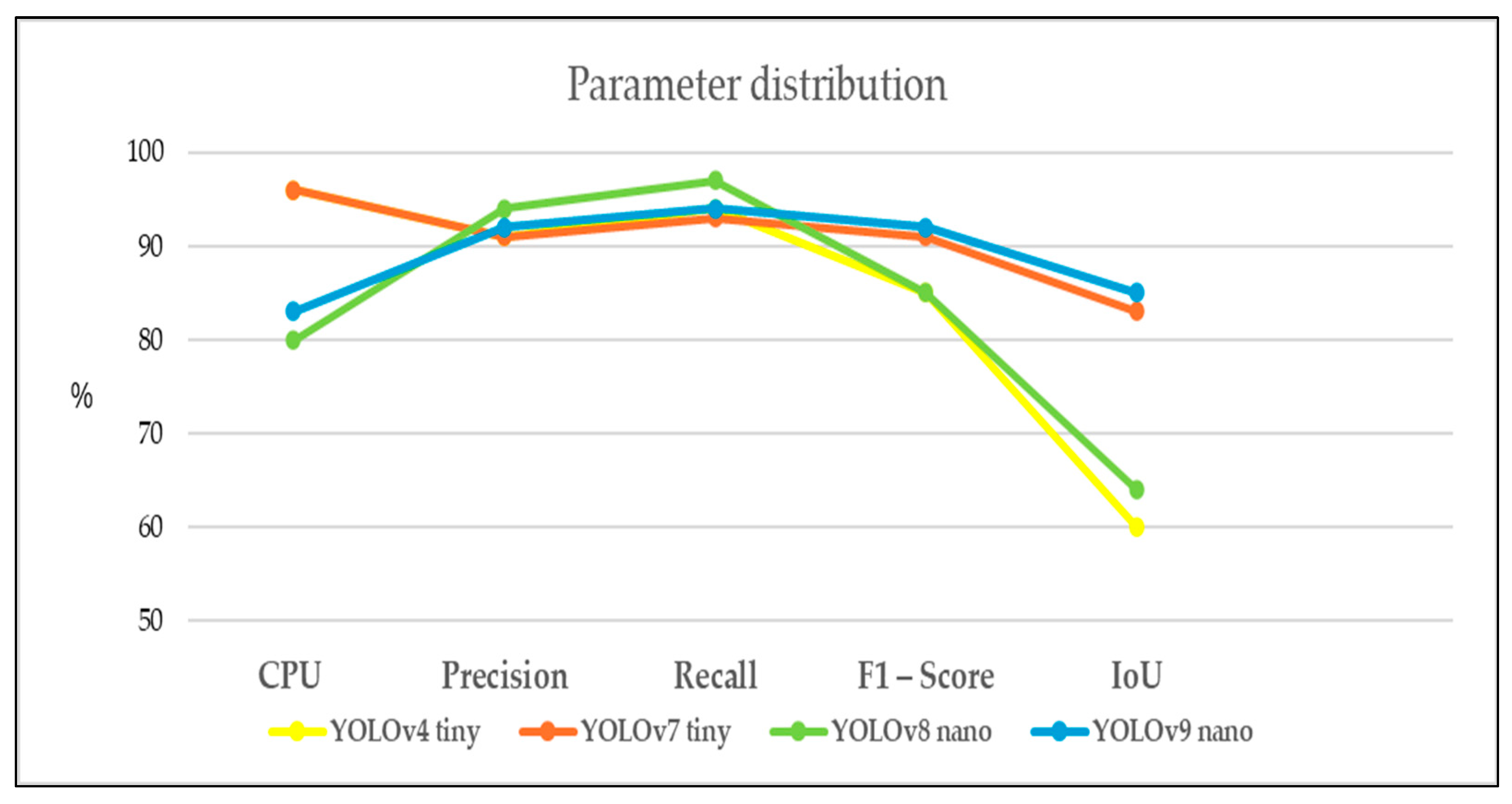
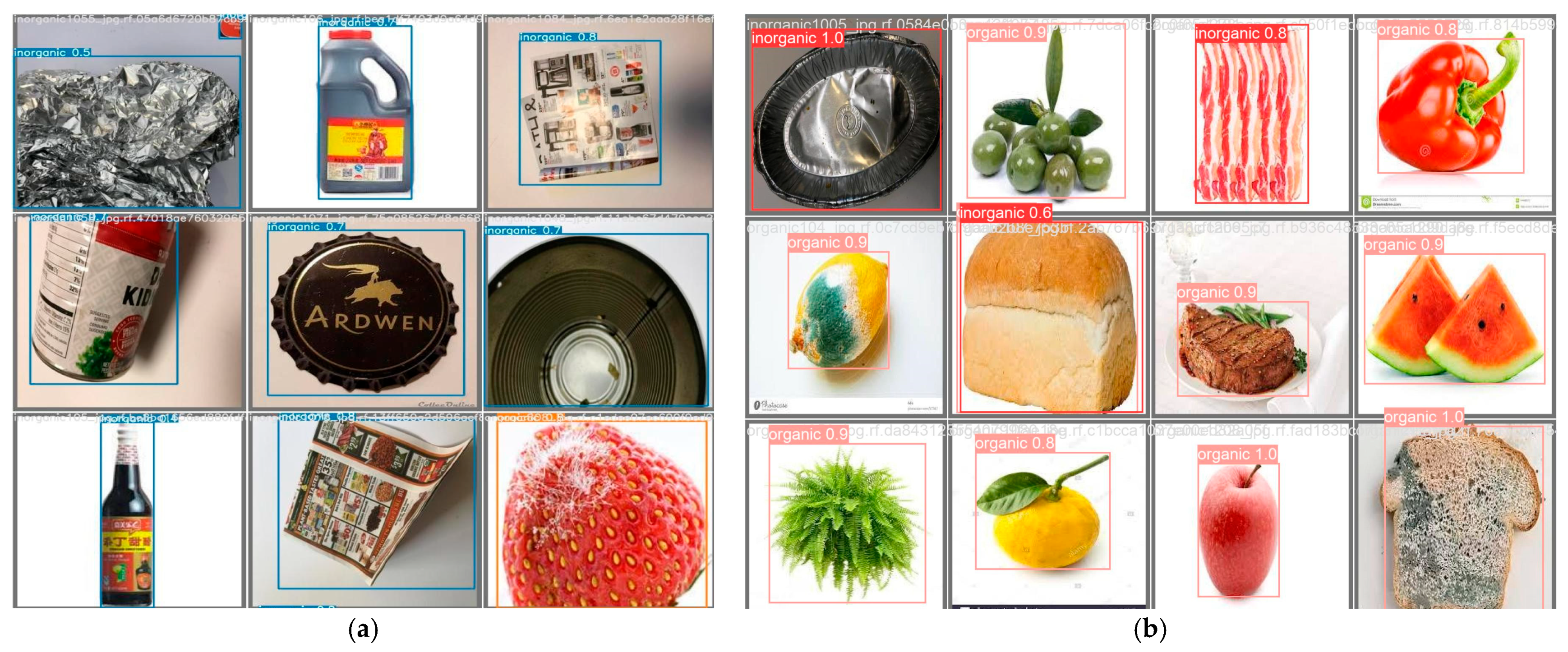
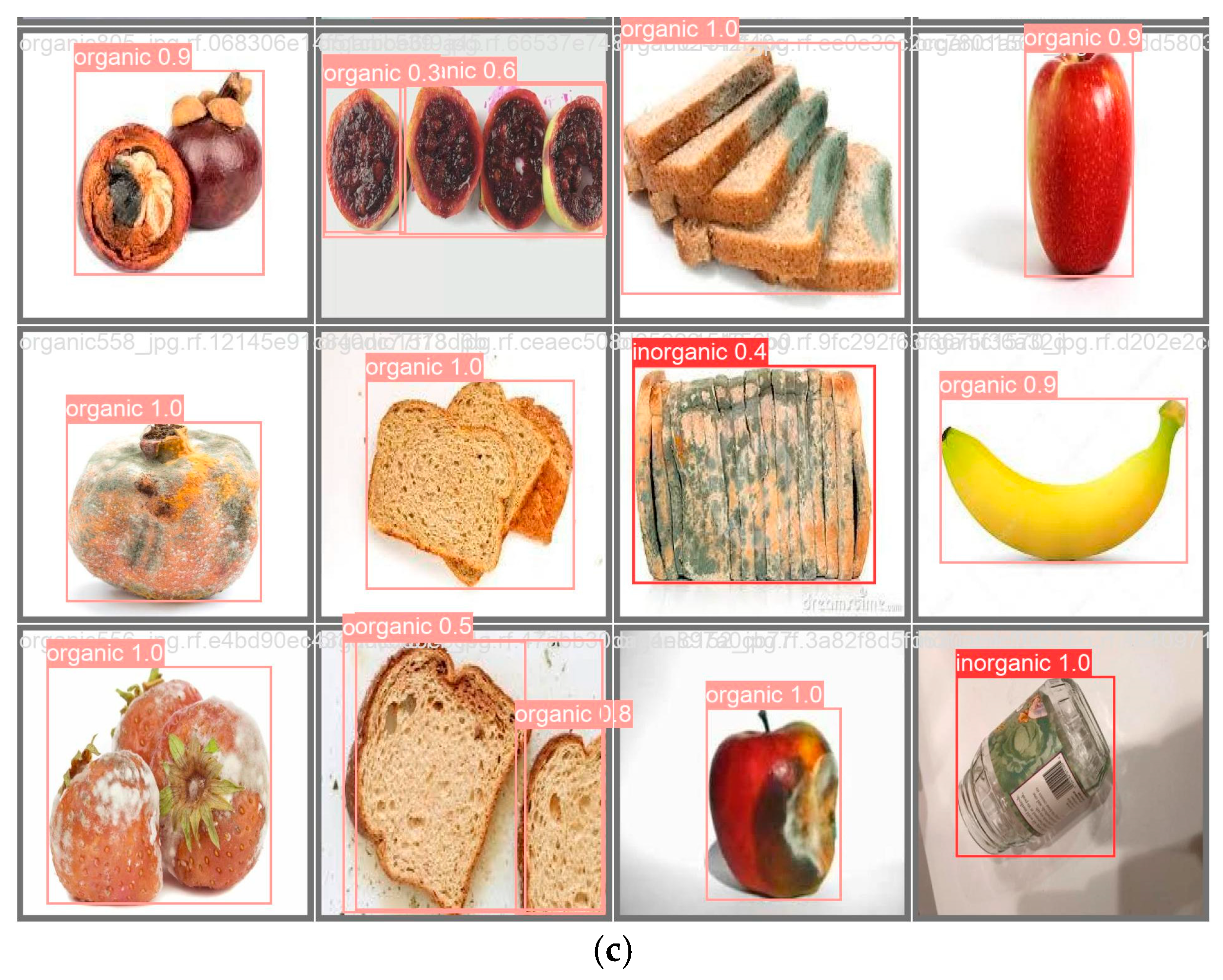
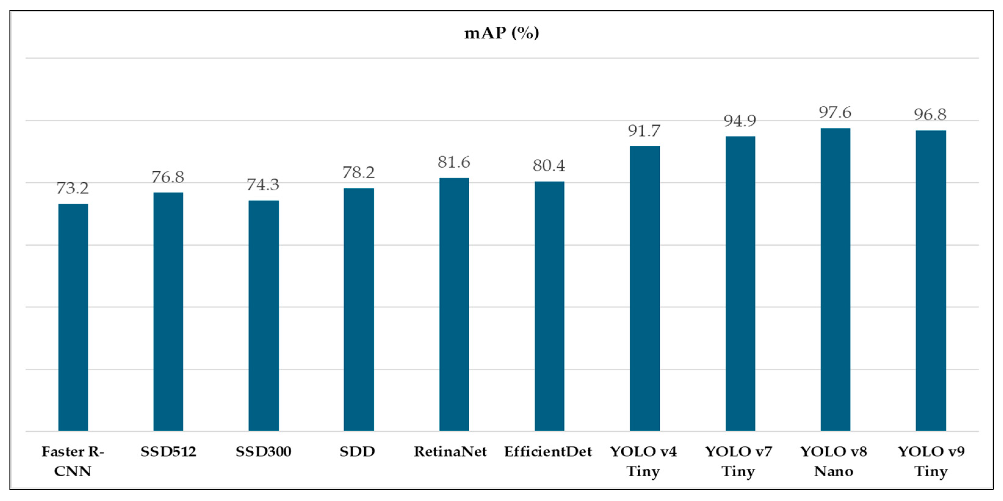
3. Results
3.1. Autonomy of Embedded System
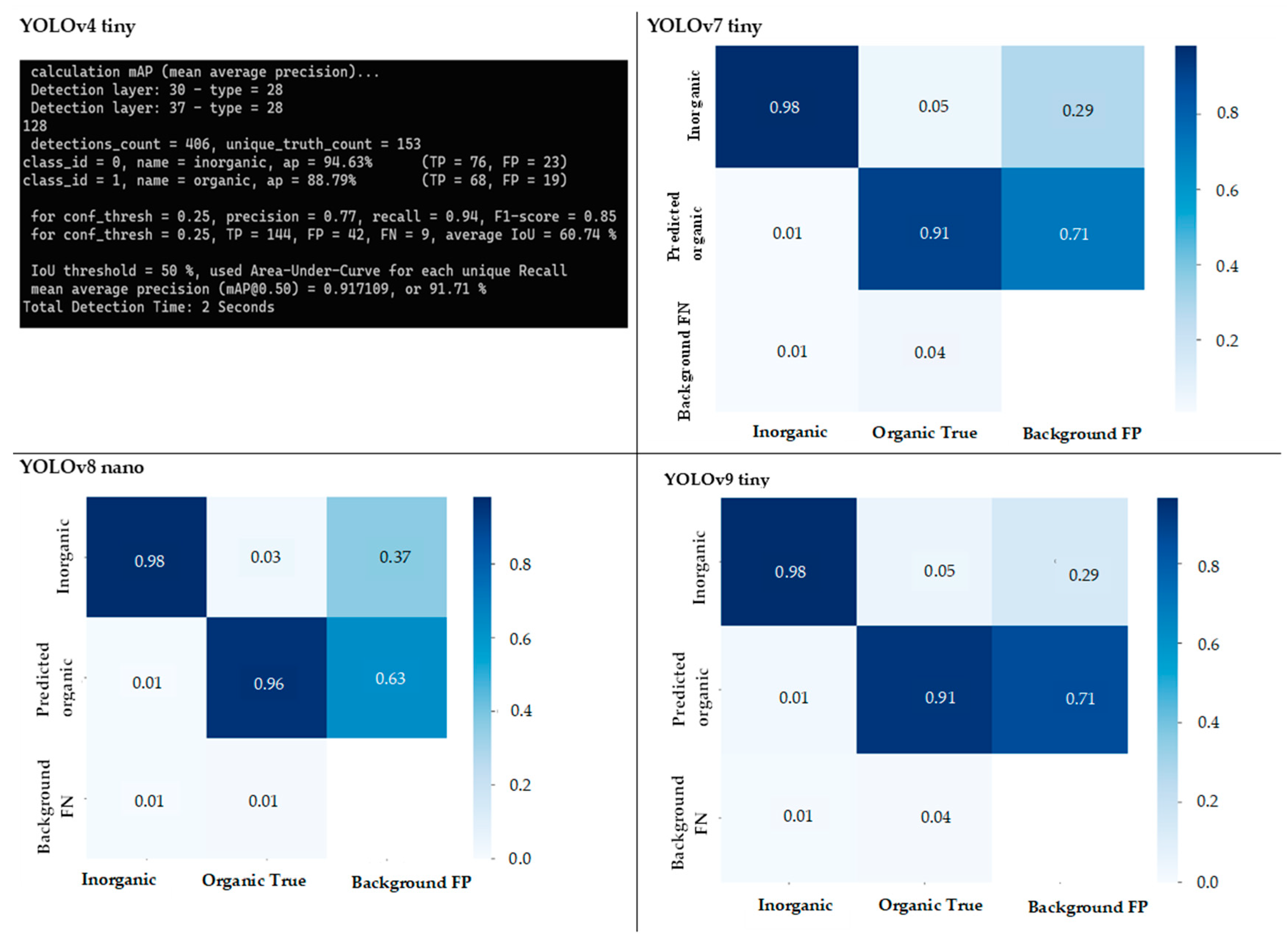
3.2. Comparison of Detection Models
4. Discussion
5. Conclusions
Author Contributions
Funding
Institutional Review Board Statement
Informed Consent Statement
Data Availability Statement
Conflicts of Interest
References
- Jin, B.; Li, W. Spatial Effects and Driving Factors of Consumption Upgrades on Municipal Solid Waste Eco-Efficiency, Considering Emission Outputs. Sustainability 2025, 17, 2356. [Google Scholar] [CrossRef]
- Zhou, Y.; Wang, Z.; Zheng, S.; Zhou, L.; Dai, L.; Luo, H.; Zhang, Z.; Sui, M. Optimization of Automated Gar-bage Recognition Model Based on ResNet-50 and Weakly Supervised CNN for Sustainable Urban Development. Alex. Eng. J. 2024, 108, 415–427. [Google Scholar] [CrossRef]
- De Carolis, B.; Ladogana, F.; Macchiarulo, N. YOLO TrashNet: Garbage Detection in Video Streams. In Proceedings of the 2020 IEEE Conference on Evolving and Adaptive Intelligent Systems (EAIS), Bari, Italy, 27–29 May 2020; pp. 1–7. [Google Scholar]
- Falaschetti, L.; Manoni, L.; Palma, L.; Pierleoni, P.; Turchetti, C. Embedded Real-Time Vehicle and Pedestrian Detection Using a Compressed Tiny YOLO v3 Architecture. IEEE Trans. Intell. Transp. Syst. 2024, 25, 19399–19414. [Google Scholar] [CrossRef]
- He, K.; Zhang, X.; Ren, S.; Sun, J. Deep Residual Learning for Image Recognition. In Proceedings of the 2016 IEEE Conference on Computer Vision and Pattern Recognition (CVPR), Las Vegas, NV, USA, 26 June–1 July 2016; pp. 770–778. [Google Scholar]
- Wang, L.; Ji, W.; Wang, G.; Feng, Y.; Du, M. Intelligent Design and Optimization of Exercise Equipment Based on Fusion Algorithm of YOLOv5-ResNet 50. Alex. Eng. J. 2024, 104, 710–722. [Google Scholar] [CrossRef]
- Chen, Z.; Yang, J.; Chen, L.; Jiao, H. Garbage Classification System Based on Improved ShuffleNet V2. Resour. Conserv. Recycl. 2022, 178, 106090. [Google Scholar] [CrossRef]
- Sachin, C.; Manasa, N.; Sharma, V.; AA, N.K. Vegetable Classification Using You Only Look Once Algorithm. In Proceedings of the 2019 International Conference on Cutting-edge Technologies in Engineering (ICon-CuTE), Uttar Pradesh, India, 14–16 November 2019; pp. 101–107. [Google Scholar]
- Liu, S.; Jin, Y.; Ruan, Z.; Ma, Z.; Gao, R.; Su, Z. Real-Time Detection of Seedling Maize Weeds in Sustainable Agriculture. Sustainability 2022, 14, 15088. [Google Scholar] [CrossRef]
- Ultralytics Ultralytics Home. Available online: https://docs.ultralytics.com/es#how-can-i-train-a-custom-yolo-model-on-my-dataset (accessed on 22 March 2025).
- Wu, Z.; Zhang, D.; Shao, Y.; Zhang, X.; Zhang, X.; Feng, Y.; Cui, P. Using YOLOv5 for Garbage Classification. In Proceedings of the 2021 4th International Conference on Pattern Recognition and Artificial Intelligence (PRAI), Yibin, China, 20–22 August 2021; pp. 35–38. [Google Scholar]
- Zeng, M.; Lu, X.; Xu, W.; Zhou, T.; Liu, Y. PublicGarbageNet: A Deep Learning Framework for Public Garbage Classification. In Proceedings of the 2020 39th Chinese Control Conference (CCC), Shenyang, China, 27–29 July 2020; pp. 7200–7205. [Google Scholar]
- Yang, Z.; Xia, Z.; Yang, G.; Lv, Y. A Garbage Classification Method Based on a Small Convolution Neural Network. Sustainability 2022, 14, 14735. [Google Scholar] [CrossRef]
- Zhang, D.; Hao, X.; Wang, D.; Qin, C.; Zhao, B.; Liang, L.; Liu, W. An Efficient Lightweight Convolutional Neural Network for Industrial Surface Defect Detection. Artif. Intell. Rev. 2023, 56, 10651–10677. [Google Scholar] [CrossRef]
- Zhang, D.; Wang, Y.; Meng, L.; Yan, J.; Qin, C. Adaptive Critic Design for Safety-Optimal FTC of Unknown Nonlinear Systems with Asymmetric Constrained-Input. ISA Trans. 2024, 155, 309–318. [Google Scholar] [CrossRef]
- Zhang, D.; Hao, X.; Liang, L.; Liu, W.; Qin, C. A Novel Deep Convolutional Neural Network Algorithm for Surface Defect Detection. J. Comput. Des. Eng. 2022, 9, 1616–1632. [Google Scholar] [CrossRef]
- Majchrowska, S.; Mikołajczyk, A.; Ferlin, M.; Klawikowska, Z.; Plantykow, M.A.; Kwasigroch, A.; Majek, K. Deep Learning-Based Waste Detection in Natural and Urban Environments. Waste Manag. 2022, 138, 274–284. [Google Scholar] [CrossRef] [PubMed]
- Laksono, P.W.; Anisa, A.; Priyandari, Y. Deep Learning Implementation Using Convolutional Neural Network in Inorganic Packaging Waste Sorting. Frankl. Open 2024, 8, 100146. [Google Scholar] [CrossRef]
- Fu, B.; Li, S.; Wei, J.; Li, Q.; Wang, Q.; Tu, J. A Novel Intelligent Garbage Classification System Based on Deep Learning and an Embedded Linux System. IEEE Access 2021, 9, 131134–131146. [Google Scholar] [CrossRef]
- Gude, D.K.; Bandari, H.; Challa, A.K.R.; Tasneem, S.; Tasneem, Z.; Bhattacharjee, S.B.; Lalit, M.; Flores, M.A.L.; Goyal, N. Transforming Urban Sanitation: Enhancing Sustainability through Machine Learning-Driven Waste Processing. Sustainability 2024, 16, 7626. [Google Scholar] [CrossRef]
- Roboflow. Available online: https://app.roboflow.com/login (accessed on 24 October 2024).
- YOLOv4. Available online: https://github.com/AlexeyAB/darknet (accessed on 22 November 2024).
- YOLOv7. Available online: https://github.com/WongKinYiu/yolov7 (accessed on 22 November 2024).
- YOLOv8. Available online: https://github.com/ultralytics/ultralytics (accessed on 24 November 2024).
- YOLOv9. Available online: https://github.com/WongKinYiu/yolov9 (accessed on 24 November 2024).
- Kraft, M.; Piechocki, M.; Ptak, B.; Walas, K. Autonomous, Onboard Vision-Based Trash and Litter Detection in Low Altitude Aerial Images Collected by an Unmanned Aerial Vehicle. Remote Sens. 2021, 13, 965. [Google Scholar] [CrossRef]
- Thung, G.; Yang, M. Classification of Trash for Recyclability Status; CS229; Stanford University: Stanford, CA, USA, 2016. [Google Scholar]
- Sashaank Sekar Waste Classification Data. Available online: https://www.kaggle.com/datasets/techsash/waste-classification-data/data (accessed on 9 December 2024).
- Mostafa Mohamed Garbage Classification (12 Classes). Available online: https://www.kaggle.com/datasets/mostafaabla/garbage-classification (accessed on 9 December 2024).
- Kumsetty, N.V.; Bhat Nekkare, A.; Kamath, S.S.; Kumar, M.A. TrashBox: Trash Detection and Classification Using Quantum Transfer Learning. In Proceedings of the 2022 31st Conference of Open Innovations Association (FRUCT), Helsinki, Finland, 27–29 April 2022; pp. 125–130. [Google Scholar]
- Redmon, J.; Divvala, S.K.; Girshick, R.B.; Farhadi, A. You Only Look Once: Unified, Real-Time Object Detection. In Proceedings of the IEEE Conference on Computer Vision and Pattern Recognition (CVPR), Nashville, TN, USA, 11–15 June 2015. [Google Scholar] [CrossRef]
- Kim, K.; Kim, K.; Jeong, S. Application of YOLO v5 and v8 for Recognition of Safety Risk Factors at Construction Sites. Sustainability 2023, 15, 15179. [Google Scholar] [CrossRef]
- Gao, X.; Wang, G.; Qi, J.; Wang, Q.; Xiang, M.; Song, K.; Zhou, Z. Improved YOLO v7 for Sustainable Agriculture Significantly Improves Precision Rate for Chinese Cabbage (Brassica Pekinensis Rupr.) Seedling Belt (CCSB) Detection. Sustainability 2024, 16, 4759. [Google Scholar] [CrossRef]
- Sallang, N.C.A.; Islam, M.T.; Islam, M.S.; Arshad, H. A CNN-Based Smart Waste Management System Using TensorFlow Lite and LoRa-GPS Shield in Internet of Things Environment. IEEE Access 2021, 9, 153560–153574. [Google Scholar] [CrossRef]
- Fu, C.-Y.; Liu, W.; Ranga, A.; Tyagi, A.; Berg, A.C. DSSD: Deconvolutional Single Shot Detector. arXiv 2017, arXiv:1701.06659. [Google Scholar] [CrossRef]
- Tan, M.; Pang, R.; Le, Q. V EfficientDet: Scalable and Efficient Object Detection. arXiv 2019, arXiv:1911.09070. [Google Scholar] [CrossRef]
- Lin, T.-Y.; Goyal, P.; Girshick, R.; He, K.; Dollár, P. Focal Loss for Dense Object Detection. arXiv 2017, arXiv:1708.02002. [Google Scholar] [CrossRef]
- Patel, D.; Patel, F.; Patel, S.; Patel, N.; Shah, D.; Patel, V. Garbage Detection Using Advanced Object Detection Techniques. In Proceedings of the 2021 International Conference on Artificial Intelligence and Smart Systems (ICAIS), Coimbatore, India, 25–27 March 2021; pp. 526–531. [Google Scholar]


| Name | No. of Categories | No. of Images | Annotation | Image Type | Author |
|---|---|---|---|---|---|
| UAVVaste | 1 (garbage waste in green areas) | 772 | Segmentation | Waste capture in open fields | [26] |
| Trashnet | 6 (glass, paper, cardboard, plastic, metal, general waste) | 2527 | Classification | Clean background or white background | [27] |
| Waste Classification data | 2 (organic and recyclable objects) | ~25,000 | Classification | Generated by Google searches | [28] |
| Garbage Classification | 12 (battery, biological, brown glass, cardboard, clothes, green glass, metal, paper, plastic, shoes, trash, white glass) | 15,150 | Classification/Detection | Combining the “clothing dataset” and the web scrapping tool | [29] |
| TrashBox | 7 (medical waste, electronic waste, plastics, paper, metal, glass, cardboard) | 17,785 | Classification/Detection | Generated by the web | [30] |
| Model Settings: YOLOv4 Tiny | Model Settings: YOLOv7 Tiny | Model Settings: YOLOv8 Nano | Model Settings: YOLOv9 Tiny | ||||
|---|---|---|---|---|---|---|---|
| Input | 640 × 640 | Input | 640 × 640 | Input | 640 × 640 | Input | 640 × 640 |
| Learning rate | 0.002 | Learning rate | 0.001 | Learning rate | 0.001 | Learning rate | 0.001 |
| Weight decay | 0.0002 | Optimizer | Adam | Optimizer | Adam | Optimizer | Adam |
| Optimizer | Adam | Momentum | 0.937 | Momentum | 0.937 | Momentum | 0.937 |
| Momentum | 0.937 | Batchsize | 32 | Batchsize | 32 | Batchsize | 32 |
| Batchsize | 32 | Subdivisions | 8 | Subdivisions | 8 | Subdivisions | 8 |
| Subdivisions | 8 | Total epoch | 100 | Total epoch | 100 | Total epoch | 100 |
| Total iterations | 6000 | ||||||
| Model | Clase | Valores | Precision | Recall | F1-Score | IoU |
|---|---|---|---|---|---|---|
| YOLOv9 tiny | Inorganic | TP = 0.97 FN = 0.19 FP = 0.04 | ||||
| Organic | TP = 0.93 FN = 0.04 FP = 0.06 |
| Model | Precision | Recall | F1-Score | IoU |
|---|---|---|---|---|
| YOLOv4 tiny | ||||
| YOLOv7 tiny | ||||
| YOLOv8 nano | ||||
| YOLOv9 tiny |
| Model | Input Resolution | mAP (%) | Model | Input Resolution | mAP (%) |
|---|---|---|---|---|---|
| Faster R-CNN [34] | ~1000 × 600 | 73.2 | SDD [35] | 513 × 513 | 78.2 |
| SSD512 [34] | 512 × 512 | 76.8 | YOLO v4 Tiny | 640 × 640 | 91.7 |
| SSD300 [34] | 300 × 300 | 74.3 | YOLO v7 Tiny | 640 × 640 | 94.9 |
| EfficientDet [36] | 1536 × 1536 | 80.4 | YOLO v8 Nano | 640 × 640 | 97.6 |
| RetinaNet [37] | 600 × 600 | 81.6 | YOLO v9 Tiny | 640 × 640 | 96.8 |
| Model | CPU Usage | Inference Time (ms) | FPS | Precision | Recall | F1-Score | Model Size (MB) | mAP@0.5 |
|---|---|---|---|---|---|---|---|---|
| YOLO v4 Tiny | 96% | 2000 | 1 | 91.71% | 94% | 0.85 | 22.4 | 0.917 |
| YOLO v7 Tiny | 98% | 1900 | 1 | 91.34% | 93.83% | 0.344 | 11.7 | 0.949 |
| YOLO v8 Nano | 86% | 1800 | 1.70 | 93% | 97.34% | 0.665 | 5.96 | 0.976 |
| YOLO v9 Tiny | 86% | 1800 | ~1.50 | 92.11% | 94.97% | 0.729 | 4.43 | 0.968 |
Disclaimer/Publisher’s Note: The statements, opinions and data contained in all publications are solely those of the individual author(s) and contributor(s) and not of MDPI and/or the editor(s). MDPI and/or the editor(s) disclaim responsibility for any injury to people or property resulting from any ideas, methods, instructions or products referred to in the content. |
© 2025 by the authors. Licensee MDPI, Basel, Switzerland. This article is an open access article distributed under the terms and conditions of the Creative Commons Attribution (CC BY) license (https://creativecommons.org/licenses/by/4.0/).
Share and Cite
Castro-Bello, M.; Roman-Padilla, D.B.; Morales-Morales, C.; Campos-Francisco, W.; Marmolejo-Vega, C.V.; Marmolejo-Duarte, C.; Evangelista-Alcocer, Y.; Gutiérrez-Valencia, D.E. Convolutional Neural Network Models in Municipal Solid Waste Classification: Towards Sustainable Management. Sustainability 2025, 17, 3523. https://doi.org/10.3390/su17083523
Castro-Bello M, Roman-Padilla DB, Morales-Morales C, Campos-Francisco W, Marmolejo-Vega CV, Marmolejo-Duarte C, Evangelista-Alcocer Y, Gutiérrez-Valencia DE. Convolutional Neural Network Models in Municipal Solid Waste Classification: Towards Sustainable Management. Sustainability. 2025; 17(8):3523. https://doi.org/10.3390/su17083523
Chicago/Turabian StyleCastro-Bello, Mirna, Dominic Brian Roman-Padilla, Cornelio Morales-Morales, Wilfrido Campos-Francisco, Carlos Virgilio Marmolejo-Vega, Carlos Marmolejo-Duarte, Yanet Evangelista-Alcocer, and Diego Esteban Gutiérrez-Valencia. 2025. "Convolutional Neural Network Models in Municipal Solid Waste Classification: Towards Sustainable Management" Sustainability 17, no. 8: 3523. https://doi.org/10.3390/su17083523
APA StyleCastro-Bello, M., Roman-Padilla, D. B., Morales-Morales, C., Campos-Francisco, W., Marmolejo-Vega, C. V., Marmolejo-Duarte, C., Evangelista-Alcocer, Y., & Gutiérrez-Valencia, D. E. (2025). Convolutional Neural Network Models in Municipal Solid Waste Classification: Towards Sustainable Management. Sustainability, 17(8), 3523. https://doi.org/10.3390/su17083523