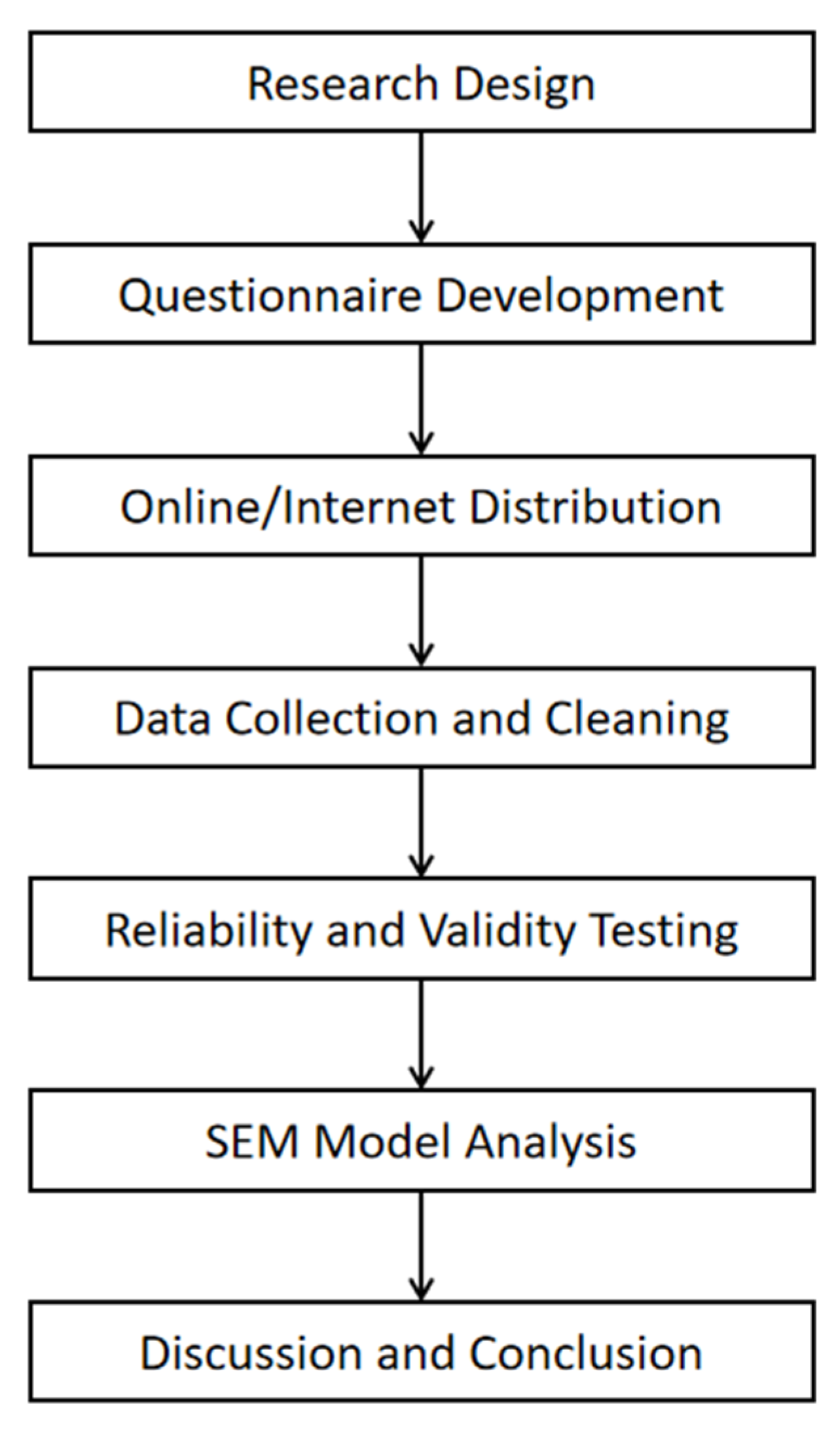
3.1. Research Method
To explore the multi-level influencing mechanisms of green perception among urban and rural residents, this study constructs a theoretical framework based on the Social Ecological Model and conducts an empirical analysis of the relationships between variables using Structural Equation Modeling (SEM). The questionnaire design uses a five-point Likert scale (1 = strongly disagree, 5 = strongly agree) to measure each latent variable. All measurement items are adapted from the existing literature and moderately revised to fit the Chinese context.
Environmental Knowledge: Includes knowledge of low-carbon living, waste sorting, climate change, etc. The items are sourced from Zhao et al. [
24].
Environmental Attitude: Measures an individual’s environmental responsibility, willingness to bear costs, and recognition of environmental values. The items are adapted from Li et al. [
47].
Family Support: Measures the influence of family members on individuals’ environmental behavior in terms of behavior and attitude. The items are adapted from Wang et al. [
38].
Social Network: Assesses the impact of social media platforms and information sharing among friends on environmental cognition. The items are sourced from Meng et al. [
40].
Community Atmosphere and Facilities: Reflects the environmental awareness of community residents and the physical environment construction of the community. The items are referenced from Zhang et al. [
8] and Shengyue Fan et al. [
65].
Policy Influence: Assesses the perceptibility, rationality, and transparency of government environmental policies; based on Wang et al. [
63].
Organizational Factors: Includes green management practices of enterprises or organizations, employee environmental awareness training, green supply chains, etc. The items are adapted from Bag, S. et al. [
73].
Green Perception: Measures an individual’s subjective attitude and self-identity in green consumption and participation in green behavior; based on Chen et al. [
80].
All variables include 3–6 items. The original data were collected through the Wenjuanxing platform and social networks, with a total of 700 samples collected. After data cleaning, 301 urban and 301 rural samples were retained for subsequent analysis.
The data analysis process is as follows: first, reliability testing (Cronbach’s α) and validity verification (KMO test, Bartlett’s test of sphericity) are conducted. Confirmatory factor analysis (CFA) and structural model construction are performed using AMOS 26.0.
Model estimation uses the Maximum Likelihood (ML) method, and model fit is evaluated through fit indices such as χ2/df, RMSEA, CFI, and TLI.
In traditional urban–rural comparative studies, rural populations are typically dominated by elderly individuals and are relatively small in number [
85]. However, due to the nature of online survey data, most respondents are under the age of 60, which differs significantly from the demographic structure of rural populations.
The classification of cities follows China’s latest urban scale classification standard, which categorizes cities into several levels—super first-tier, first-tier, second-tier, third-tier, and lower—based on permanent population and economic development level [
86].
This classification provides a scientific basis for describing the distribution and background of the research sample, ensuring data representativeness and broad applicability.
China’s household registration system underwent a major reform in 2014, abolishing the distinction between agricultural and non-agricultural household registrations. However, due to the long-term accumulation of socio-economic conditions in urban and rural areas, significant differences remain in housing, employment, and social welfare between urban and rural populations. Therefore, in urban–rural comparative studies, respondents’ household registration origins (i.e., whether they were born into an agricultural household) can still be used to measure their socio-economic background.
The Regulations on the Statistical Division of Urban and Rural Areas clearly state that “based on China’s administrative divisions, using the jurisdictions of residents’ committees and village committees confirmed by the civil affairs department as the division objects, and actual construction as the division criterion, China is divided into urban and rural areas”.
Among them, “urban areas include urban districts and town districts. Urban districts refer to areas in municipal districts and county-level cities where actual construction is connected to residents’ committees and other areas within the jurisdiction of the district or city government”. “Town districts refer to areas outside urban districts, including county government seats and other towns where actual construction is connected to residents’ committees and other areas within the jurisdiction of the town government”. “Rural areas refer to regions outside the urban areas as defined by these regulations”.
Therefore, this study adopts a classification scheme that distinguishes between agricultural households based on rural areas and non-agricultural households based on urban and town districts as an alternative approach to urban–rural comparison. This classification method is reasonable and valid.
In the questionnaire samples collected for this study, urban residents accounted for 57%, slightly lower than the proportion of the urban population (65.22%) published by the National Bureau of Statistics in 2022 [Source: “China Statistical Yearbook [
87]”]. Although it is generally believed that questionnaire collection in rural areas is more difficult, in this study, the efficiency of collecting rural samples was slightly higher than that of urban samples. This phenomenon is mainly due to differences in questionnaire distribution strategies; urban residents, due to frequent exposure to online questionnaires, generally experience participation fatigue or information filtering tendencies [
87], while rural residents receive questionnaires through familiar social networks such as “WeChat Elderly Groups”, leading to higher participation willingness and better completion rates [
88]. At the same time, some rural respondents reported that the environmental protection topics covered in the questionnaire were closely related to their daily lives, especially in the context of increasingly significant changes in the rural ecological environment, which triggered a stronger sense of identification and motivation to complete the questionnaire. In contrast, while urban residents have more extensive information channels, the distribution of questionnaires is more random, and coupled with information overload, the response rate is relatively lower. Based on the research objective of comparing urban and rural green perception pathways, this study ultimately selected 301 questionnaire samples from urban and rural areas, respectively, in accordance with the principle of urban–rural balance from all valid samples, for Structural Equation Modeling analysis, and to ensure the stability of model estimation and the feasibility of comparing urban and rural samples.
After questionnaire collection, samples were manually classified based on urban–rural divisions into two categories: agricultural households based on rural areas and non-agricultural households based on urban and town districts. The questionnaire covers multi-level influencing factors of green perception, including the individual level (e.g., environmental knowledge, environmental attitudes), social relationship level (e.g., family support, social networks), community level (e.g., community atmosphere, community facilities), policy level, and organizational level.
Data collection took place from December 2024 to February 2025, with a total of 700 questionnaires distributed and 602 valid responses collected, yielding a response rate of 86%. This exceeds the typical social science research standard, which requires a valid response rate of no less than 70% [
89], providing a reliable basis for analyzing differences in green perception between urban and rural areas (See
Table A1 and
Figure 2).
3.4. Validity Analysis
This study measured key factors using a scale and conducted reliability analysis on the questionnaire with SPSS Statistics 22.0. The KMO value was 0.925 (>0.8), and Bartlett’s test of sphericity was significant at 0.000 (<0.001), indicating that the data were suitable for factor analysis, supporting further factor extraction and model validation.
According to Ahrens et al. the KMO test and Bartlett’s test of sphericity are critical steps for verifying data suitability and construct validity, ensuring the scientific rigor and robustness of factor analysis results [
90] (See
Table 3).
Through principal component analysis and Kaiser-normalized maximum variance rotation, six distinct components were extracted, with high factor loadings (>0.7) and low cross-loadings, indicating good component independence, a stable model structure, and strong explanatory power.
This is consistent with the findings of Xiong, M. et al., who stated that KMO and Bartlett’s tests in factor analysis are effective methods for ensuring variable independence and suitability [
91] (See
Table 4).
Based on the good fit of the exploratory factor analysis results, a further model fit test was conducted. According to the model fit test results in the table, CMIN/DF (Chi-square to degrees of freedom ratio) = 1.760, which falls within the acceptable range of 1 to 3. RMSEA (Root Mean Square Error of Approximation) = 0.036, which falls within the good fit range of less than 0.05. Additionally, the results of IFI, TLI, CFI, and GFI all exceed 0.9, indicating an excellent fit. Therefore, based on the overall analysis results, the CFA model demonstrates good fit [
92] (See
Table 5).
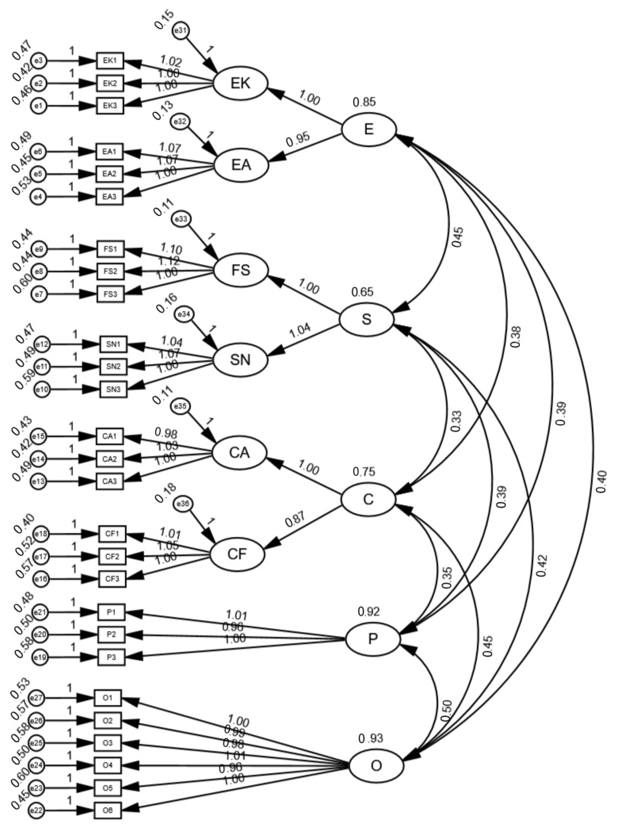
Additionally, the CFA results indicate that this study utilized Structural Equation Modeling (SEM) to validate the measurement model, with the results presented in the table. The table illustrates the convergent validity and composite reliability of the study variables, which are used to assess the reliability and validity of the measurement model.
First, convergent validity is evaluated using the Average Variance Extracted (AVE). AVE reflects the average level of variance in the measurement variables that can be explained by the latent variable. Typically, an AVE value greater than 0.5 indicates that the measurement items can adequately explain the variance of the latent variable.
As seen in the table, the AVE values for all variables range from 0.613 to 0.692, exceeding the 0.5 threshold. This indicates that the measurement model has good convergent validity, meaning the measurement items are strongly correlated and effectively measure their corresponding latent variables.
Second, composite reliability (CR) is used to assess the internal consistency of the measurement model and evaluate the overall reliability of the measurement items for each latent variable. A CR value greater than 0.7 is generally required to indicate that the scale has sufficient internal consistency.
The table shows that the CR values for all variables range from 0.826 to 0.911, meeting this standard. This indicates that the measurement items for each variable exhibit good consistency and stability, confirming the high internal consistency of the scale.
Additionally, the table includes standardized factor loadings (Estimate), which measure the correlation between each measurement item and its corresponding latent variable. Typically, a standardized factor loading greater than 0.7 is required to ensure the reliability of a measurement item.
As shown in the table, all measurement items have factor loadings greater than 0.75, meeting the standard. This indicates that these items effectively measure their respective latent variables, further supporting the convergent validity of the measurement model.
According to Bollen’s theoretical standards, the composite reliability (CR) and average variance extracted (AVE) for each latent variable were calculated [
93]. The results show that all indicators meet or exceed the recommended thresholds, confirming that the scale has good convergent validity and discriminant validity.
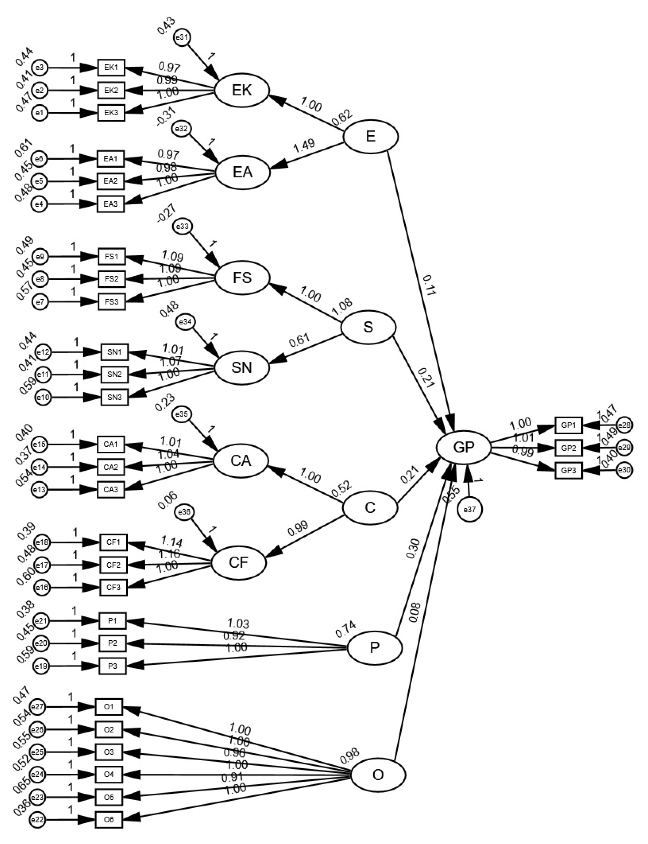
Therefore, in summary, the measurement model in this study meets high standards for both convergent validity and composite reliability, demonstrating that the measurement of research variables is reliable and valid, providing a solid foundation for subsequent Structural Equation Modeling (SEM) analysis (See
Table 6 and
Figure 3).
The formulas for calculating AVE and CR are as follows:
AVE (Average Variance Extracted):
CR (Composite Reliability):
This study employs the HTMT (Heterotrait–Monotrait Ratio) method to test discriminant validity, avoiding the applicability issues of the traditional Fornell–Larcker criterion in Higher-Order Factor Models [
94].
Since this study’s model includes second-order latent variables, AMOS only provides the correlation matrix for second-order latent variables, making it difficult for the Fornell–Larcker method to calculate the AVE (Average Variance Extracted) for all latent variables, thereby affecting the assessment of discriminant validity.
Therefore, the HTMT method is adopted to measure the correlation between measurement items of different latent variables and calculate the Heterotrait–Monotrait Ratio, providing a more accurate evaluation of discriminant validity among latent variables.
The formula for HTMT calculation is
According to the HTMT evaluation criteria, when the HTMT value is below 0.85 (strict standard) or 0.90 (lenient standard), the measurement model is considered to have good discriminant validity. In this study, the HTMT values were calculated based on the standardized correlation matrix output by AMOS, and all HTMT values were below 0.85, indicating sufficient discriminant validity among the latent variables in the model. Therefore, the HTMT method provides a more reliable discriminant validity test for the measurement model in this study, ensuring the construct validity of the model (See
Table 7).
According to the standard proposed by Kline, if the absolute value of the skewness coefficient is within 3 and the absolute value of the kurtosis coefficient is within 8, the data can be considered to meet the requirement of approximate normal distribution [
95].
This study presents the descriptive statistical analysis and normality test results for the factors used. According to the descriptive statistical analysis results, the table presents the descriptive statistical analysis and normality test results for each measurement item, including mean (Mean), standard deviation (Standard Deviation, SD), variance (Variance), skewness (Skewness), and kurtosis (Kurtosis).
Overall, the mean values for most measurement items range from 3.4 to 3.9, indicating that respondents’ attitudes toward the measured variables are moderately positive. The standard deviation ranges from 1.07 to 1.23, indicating a certain degree of data dispersion.
In terms of skewness, all measurement items have negative skewness values, indicating a left-skewed distribution overall, meaning respondents’ ratings are more concentrated in the higher score range. Most kurtosis values are close to 0 or negative, suggesting that the data distribution is relatively flat, without severe kurtosis issues. This indicates that the data generally meet the assumption of normal distribution.
The overall mean (Overall M) and overall standard deviation (Overall SD) provide a summary of each dimension, which is consistent with the mean and standard deviation of individual measurement items, indicating that the data within each dimension are relatively stable.
Based on these results, the data distribution appears reasonable and meets the normality assumptions required for subsequent Structural Equation Modeling (SEM) or regression analysis, making it suitable for further empirical analysis (See
Table 8).
3.6. Structural Equation Modeling (SEM)
In the quantitative analysis phase, this study employs Structural Equation Modeling (SEM) to test the path relationships between hypotheses. SEM is a statistical method capable of simultaneously analyzing complex relationships among multiple variables, making it suitable for both exploratory and confirmatory research.
Following the SEM modeling guidelines and model fit criteria proposed by Hair et al., this study utilizes AMOS 26.0 software for model estimation to ensure the significance of path coefficients and the overall model fit [
98].
To ensure the rationality of the Structural Equation Model (SEM), this study conducts a model fit test using key fit indices, including CMIN/DF, GFI, TLI, CFI, RMSEA, and IFI. According to model fit standards, a CMIN/DF value between 1 and 3, GFI, TLI, CFI, and IFI values above 0.9, and an RMSEA value below 0.05 indicate a well-fitting model. The SEM fit test results in this study are CMIN/DF = 1.899, GFI = 0.922, TLI = 0.964, CFI = 0.968, RMSEA = 0.039, and IFI = 0.968, all meeting the excellent fit criteria, indicating a high overall model fit. Therefore, the SEM constructed in this study is well-structured and effectively explains the relationships between variables (See
Table 10).
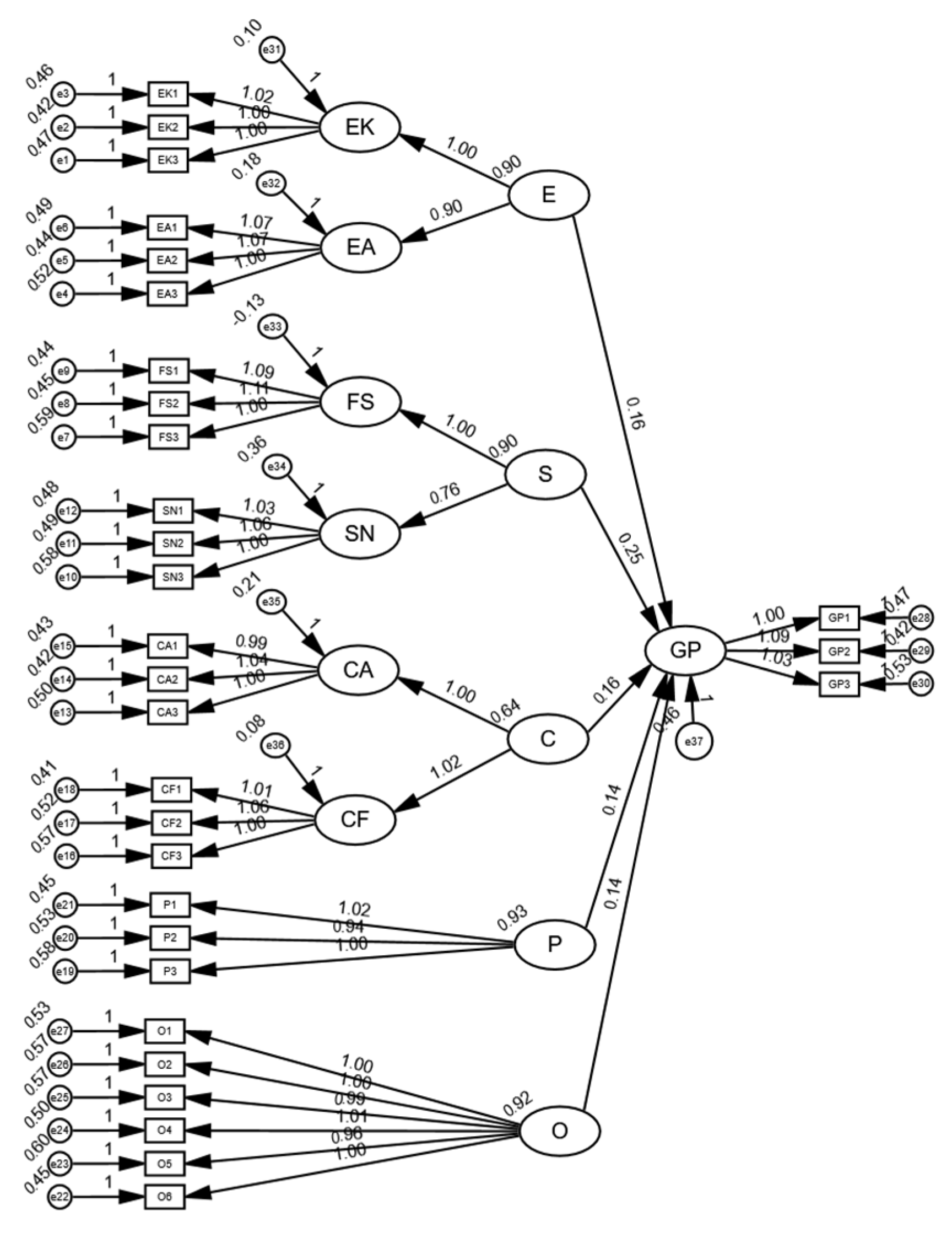
This study employs Structural Equation Modeling (SEM) to verify the effects of latent variables on green perception (GP). The path analysis results include standardized path coefficients (Estimate), standard errors (S.E.), critical ratios (C.R.), and significance levels (p-values). According to statistical standards, a path relationship is considered significant when p < 0.05.
The results of this study show that the individual level (E), interpersonal level (S), community level (C), policy level (P), and organizational level (O) all have significant positive effects on green perception (GP) (p < 0.05), confirming all proposed hypotheses. Among them, the interpersonal level (S) has the most significant effect on green perception (β = 0.252, p < 0.001), indicating that interpersonal relationship factors play a key role in shaping individual green perception. In addition, the individual level (β = 0.158, p < 0.001), community level (β = 0.158, p < 0.001), policy level (β = 0.140, p < 0.001), and organizational level (β = 0.145, p < 0.001) also have positive effects on green perception, although the magnitudes of these effects vary slightly.
Overall, the SEM results of this study support the theoretical hypotheses and confirm the promoting effects of the individual, interpersonal, community, policy, and organizational levels on green perception, thus supporting hypotheses H1, H2, H3, H4, and H5.
This finding provides empirical support for a deeper understanding of the formation mechanism of individual green perception and offers insights for policy-making and practical applications (See
Table 11 and
Figure 4).
3.7. Urban–Rural Comparative Analysis
This study used Structural Equation Modeling (SEM) to separately examine the influencing factors of green perception (GP) among urban and rural residents and conducted a comparative analysis of their path relationships. Overall, there are certain similarities in the mechanisms influencing green perception between urban and rural areas, but structural differences are also evident.
In both the urban and rural models, the interpersonal level (S) has a significant positive effect on green perception (urban: β = 0.260,
p < 0.001; rural: β = 0.214,
p = 0.005). This indicates that, whether in urban or rural areas, individuals’ social interactions and support from family, friends, or communities enhance residents’ green perception to a certain extent [
39].
Moreover, the policy level (P) has a significant effect on green perception in the rural model (β = 0.298,
p < 0.001), but is not significant in the urban model (
p = 0.533), which may be related to the directness of policy implementation and stronger government-led promotion in rural areas [
65].
The individual level (E) has a significant positive effect on green perception in the urban model (β = 0.256,
p < 0.001), but is not significant in the rural model (
p = 0.062). This reflects that urban residents are more likely to access environmental knowledge through education, media, and social networks, thereby enhancing green perception, whereas rural residents may face limitations in information dissemination channels and have relatively less access to environmental knowledge, affecting their cognitive level [
32].
The community level (C) has a significant impact on green perception in the urban model (β = 0.102,
p = 0.057), while the impact is weaker in the rural model (β = 0.205,
p = 0.011). This is because urban communities have more developed environmental atmospheres, public facilities, and the promotion of sustainable lifestyles, which help foster green awareness, whereas rural community influence may be more dispersed and weaker [
49].
The organizational level (O) significantly affects green perception in the urban model (β = 0.204,
p = 0.006) but is not significant in the rural model (
p = 0.133). This suggests that urban environmental development, green infrastructure, and city-level development policies contribute more to enhancing residents’ green perception, while rural residents’ green cognition is less influenced by organizational factors [
79].
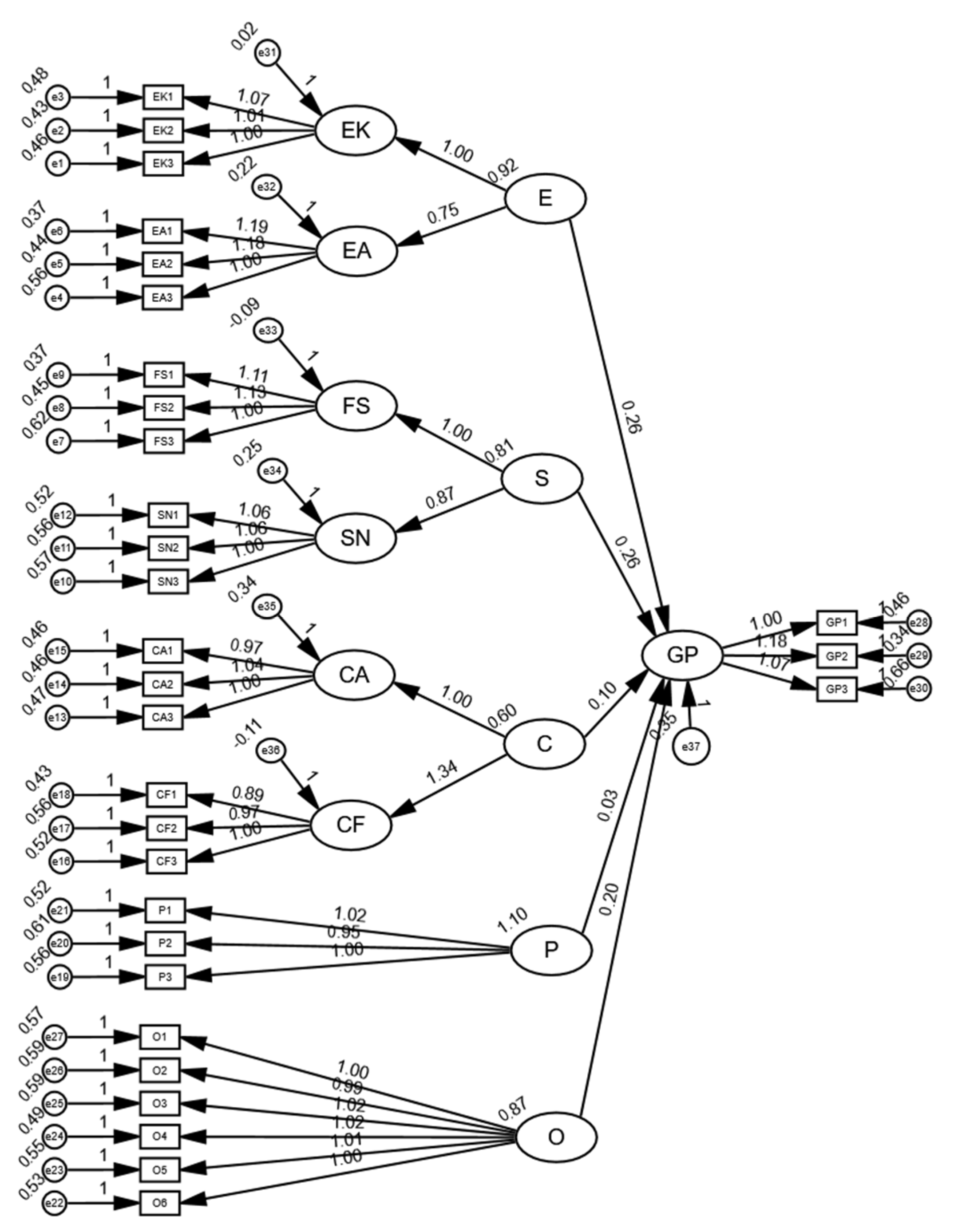
3.8. Urban SEM Model Fit Test Results and Path Relationship Hypothesis Testing Results
The model test results show that CMIN/DF = 1.666, GFI = 0.871, TLI = 0.948, CFI = 0.954, RMSEA = 0.047, and IFI = 0.955. Among these, CMIN/DF, TLI, CFI, IFI, and RMSEA all meet the excellent fit criteria, while GFI is 0.871, falling within the acceptable fit range. Overall, the model demonstrates a high level of fit, meeting the SEM fit standards, which indicates that the model structure is reasonable and effectively explains the data (See
Table 12).
The results show that the individual level (E), interpersonal level (S), and organizational level (O) all have significant positive effects on green perception (GP) (p < 0.01), supporting the corresponding hypotheses. Among these, the individual level (β = 0.256, p < 0.001) and the interpersonal level (β = 0.260, p < 0.001) have more pronounced effects on green perception, indicating that personal environmental knowledge and social interaction play a key role in enhancing green perception. In addition, the organizational level (β = 0.204, p < 0.001) also influences green perception to some extent, suggesting that the urban environment may affect individuals’ formation of green cognition, thus supporting hypotheses H1, H2, and H5.
However, the community level (C) and policy level (P) do not have significant effects on green perception (
p > 0.05), and the corresponding hypotheses are not supported. This suggests that in the urban model, community atmosphere and policy factors may not significantly influence individual green perception, which could be related to specific urban governance patterns, the strength of policy implementation, or individual perception differences. In summary, the SEM results of this study partially support the theoretical hypotheses, indicating that environmental knowledge, social support, and organizational factors are important influences on green perception, while the impacts of community atmosphere and policy factors were not significantly confirmed in this study. These findings provide empirical support for further optimizing urban sustainable development strategies (See
Table 13 and
Figure 5).
3.9. Rural SEM Model Fit Test Results and Path Relationship Hypothesis Testing Results
The rural SEM model fit test results in this study are CMIN/DF = 1.445, GFI = 0.894, TLI = 0.964, CFI = 0.968, RMSEA = 0.047, and IFI = 0.968. Among these, CMIN/DF, TLI, CFI, IFI, and RMSEA all meet the excellent fit criteria, while GFI is 0.894, which is close to the excellent fit standard but still within the acceptable fit range. Overall, the model demonstrates a high level of fit, meeting the fit standards of Structural Equation Modeling (SEM), indicating that the model effectively explains the relationships between variables and provides a reliable theoretical foundation for subsequent path analysis (See
Table 14)
The model results indicate that the interpersonal level (S) and policy level (P) have significant positive effects on green perception (GP) (p < 0.01), supporting the corresponding hypotheses. Among them, the policy level (β = 0.298, p < 0.001) and interpersonal level (β = 0.214, p = 0.005) are key influencing factors of rural residents’ green perception, indicating that policy measures and social interaction play crucial roles in fostering green awareness in rural areas. Additionally, the community level (C) has a significant effect on green perception at the P = 0.011 level, suggesting that community atmosphere exerts a certain influence on green perception, thus supporting hypotheses H2, H3, and H4.
However, the individual level (E) and organizational level (O) do not significantly influence green perception (
p > 0.05), and the corresponding hypotheses are not supported. This suggests that in rural contexts, individual environmental knowledge and organizational factors may not directly affect green perception, which could be related to rural residents’ lifestyles, information access channels, and mechanisms of environmental cognition formation. Overall, the SEM results for rural areas partially support the theoretical hypotheses, confirming the important role of social support and policy in promoting green perception among rural residents, while the effects of environmental knowledge and organizational factors were not significantly validated. This finding provides important empirical evidence for the formulation of rural sustainable development policies (See
Table 15 and
Figure 6).


