
Geothermal Genesis Mechanism of the Yinchuan Basin Based on Thermal Parameter Inversion


Abstract
:1. Introduction
2. Regional Geology and Geothermal Overview of the Ningxia Basin
3. Data and Methods
3.1. Data Description
3.2. Geothermal Parameter Modeling
3.3. MCMC Inversion
- (1)
- Arbitrarily choose an initial value and set ;
- (2)
- Generate a candidate value from the proposal distribution ;
- (3)
- Calculate the acceptance probability:where is the target probability density function;
- (4)
- Draw from . If , set ; otherwise, set ;
- (5)
- Increase and return to step 2.
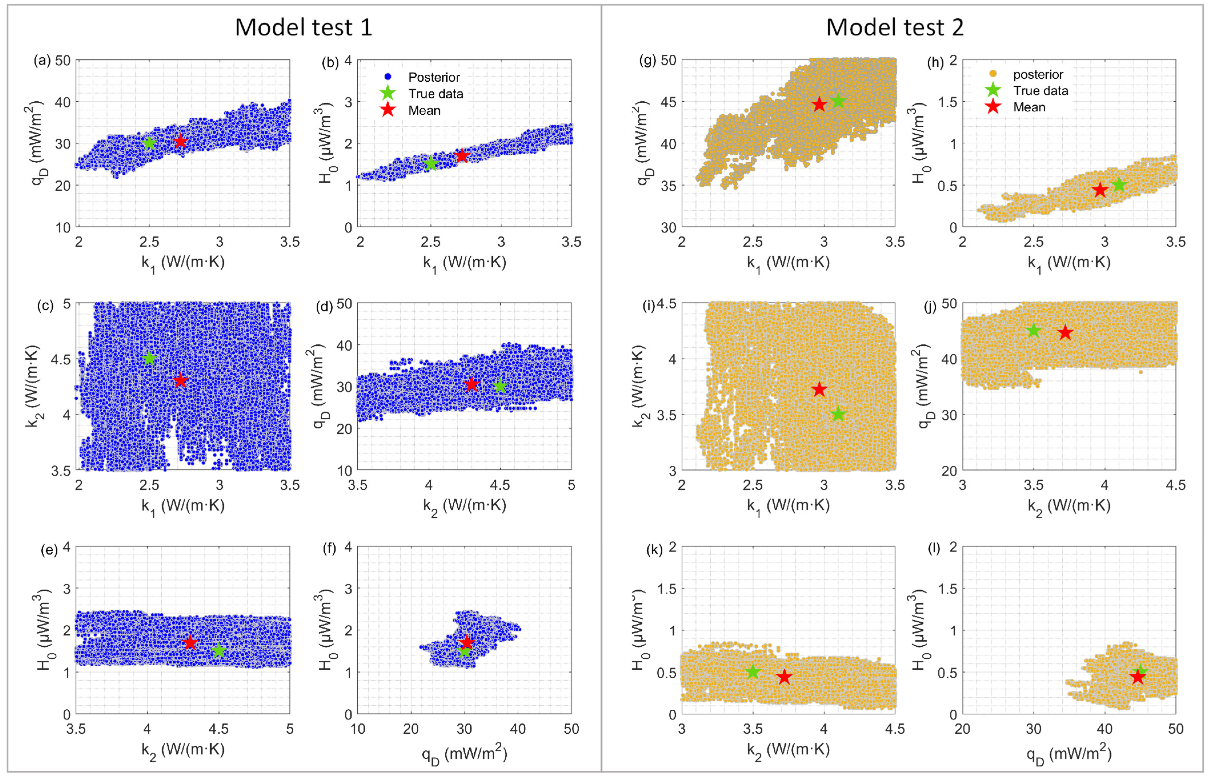
3.4. Model Test
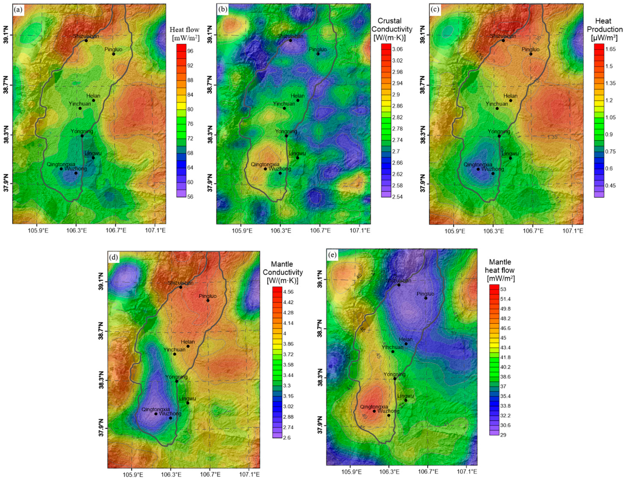
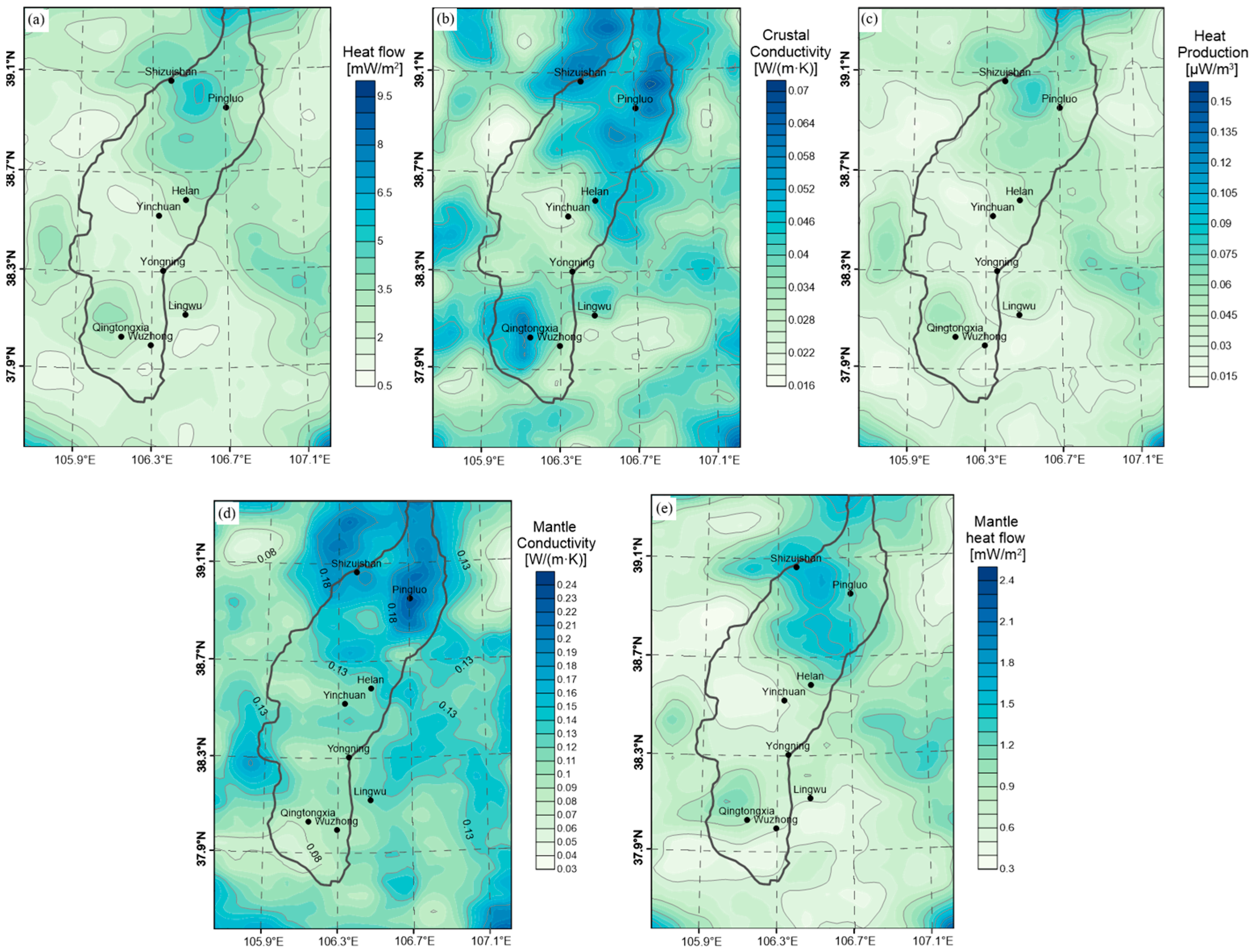
4. Results
5. Discussion
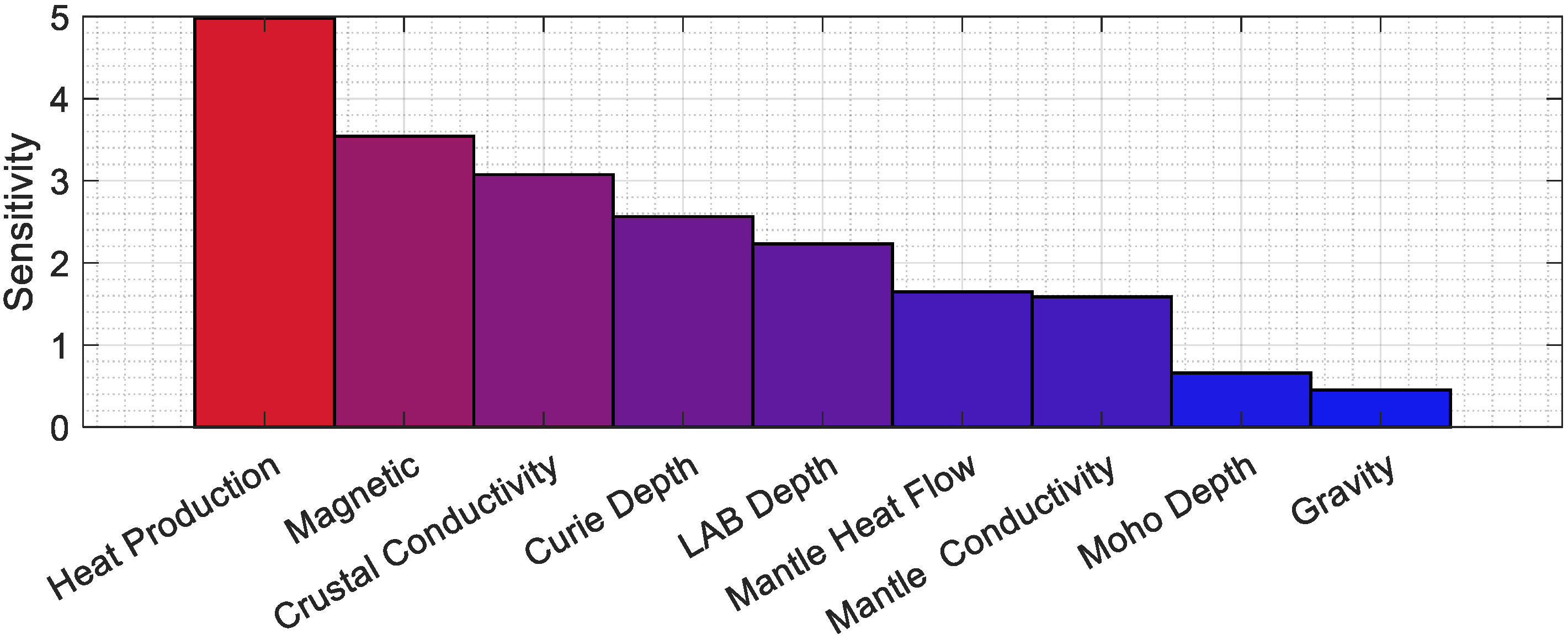
5.1. Correlation and Sensitivity Analysis
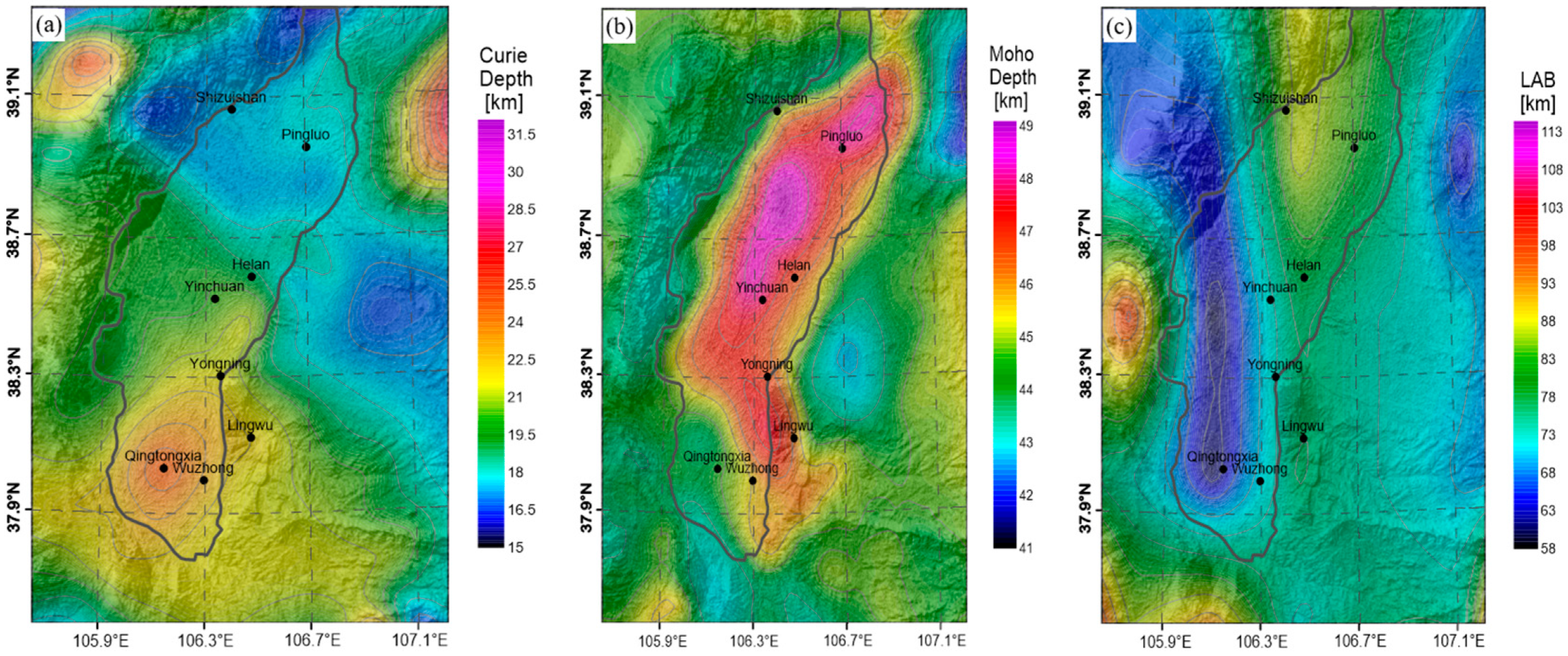
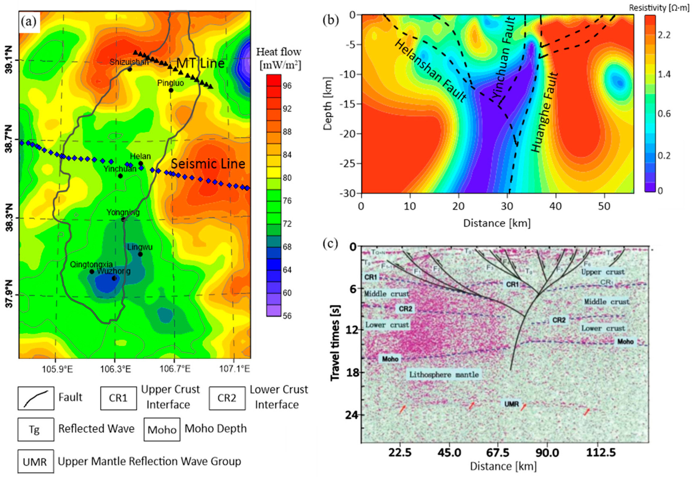
5.2. Geophysical Investigation and Analysis of Yinchuan Basin
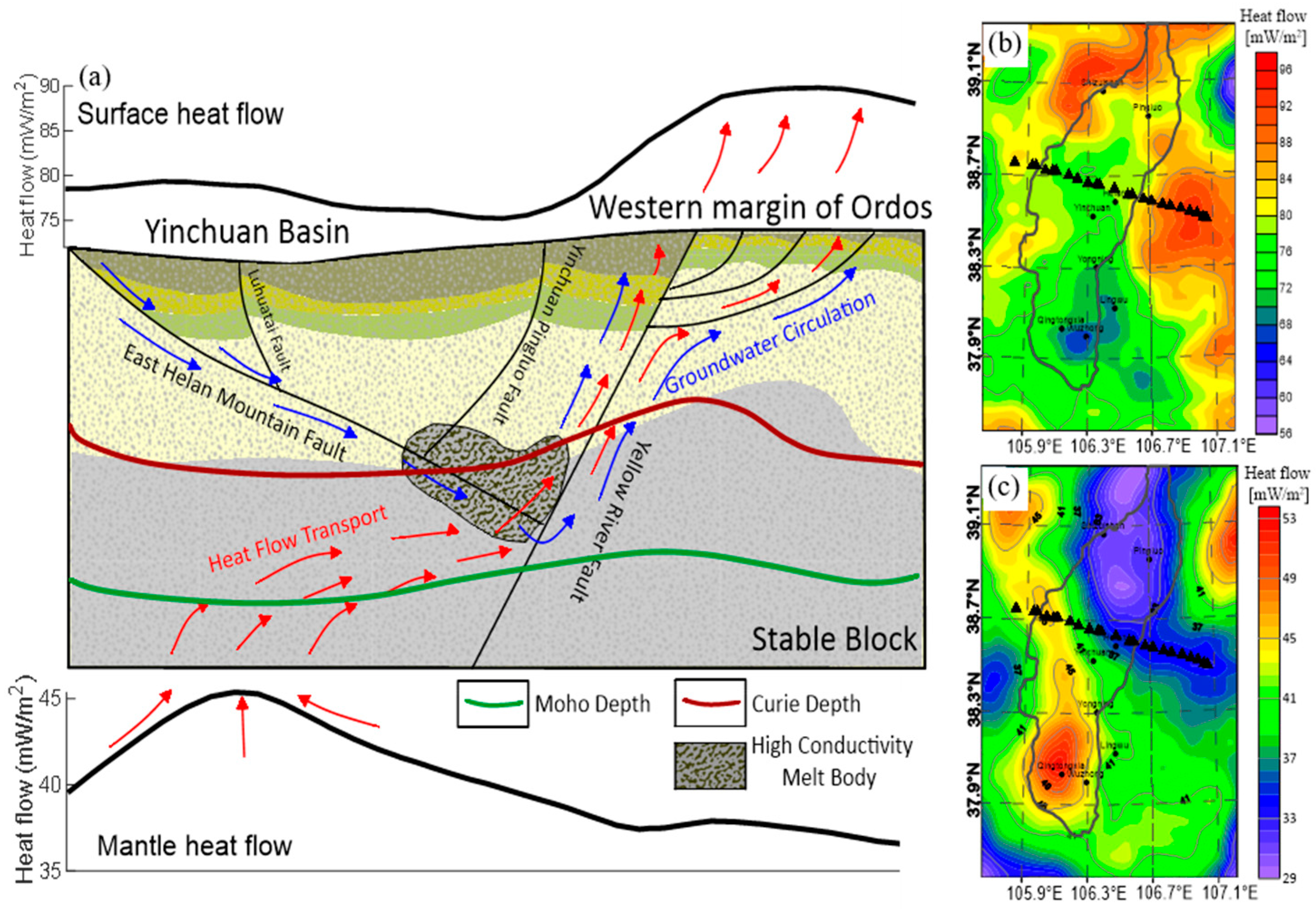
5.3. Comprehensive Interpretation of Yinchuan Basin
6. Conclusions
Author Contributions
Funding
Institutional Review Board Statement
Informed Consent Statement
Data Availability Statement
Conflicts of Interest
References
- Zhang, C.; Hu, S.; Zhang, S.; Li, S.; Zhang, L.; Kong, Y.; Zuo, Y.; Song, R.; Jiang, G.; Wang, Z. Radiogenic heat production variations in the Gonghe Basin, northeastern Tibetan Plateau: Implications for the origin of high-temperature geothermal resources. Renew. Energy 2020, 148, 284–297. [Google Scholar] [CrossRef]
- Zhang, S.Q.; Wu, H.D.; Zhang, Y.; Song, J.; Zhang, L.Y.; Xu, W.L.; Li, D.P.; Li, S.T.; Jia, X.F.; Fu, L.; et al. Characteristics of regional and geothermal geology of the Reshuiquan HDR in Guide County, Qinghai Province. Acta Geol. Sin. 2020, 94, 1591–1605, (In Chinese with English abstract). [Google Scholar]
- Yu, Q.S.; Zhou, W.S. Evaluation and Zoning of the Current Situation of Geothermal Resources in Ningxia; Ningxia Hui Autonomous Region Geological Survey: Yinchuan, China, 2014; (In Chinese with English abstract). [Google Scholar]
- Wang, L.; Zhang, L. Geothermal geological characteristics of Yinchuan Basin. In Collection of Research Papers on the Development Strategy of Geothermal Resources in Western China; Geothermal Professional Committee of China Energy Research Association: Beijing, China, 2001; pp. 44–53. [Google Scholar]
- Zhu, H.L.; Liu, Z.L.; Cao, X.G.; Xu, B.; Yang, Z.; Cheng, G.; Li, L.; Shao, B.; Zhao, C. Prospective evaluation of geothermal resource exploration on the eastern margin of the Yinchuan Basin based on magnetotelluric sounding and drilling detection. Geol. Explor. 2020, 56, 1287–1295, (In Chinese with English abstract). [Google Scholar]
- Chen, X.J.; Hu, X.J.; Li, N.S.; Wu, Y.; Cheng, G.Q.; Ni, P.; Cao, Y.Y.; Bo, J.B. Discussion on the geothermal accumulation model on the eastern margin of the Yinchuan Basin. Geophys. Geochem. Explor. 2021, 45, 583–589, (In Chinese with English abstract). [Google Scholar]
- Yang, Z.X.; Duan, Y.H.; Wang, F.Y.; Zhao, J.R.; Pan, S.Z.; Li, L. Three-dimensional transmission imaging of deep seismic faults in the Yinchuan Basin. Chin. J. Geophys. 2009, 52, 2026–2034, (In Chinese with English abstract). [Google Scholar]
- Liu, B.J.; Feng, S.Y.; Ji, J.F.; Wang, S.J.; Zhang, J.S.; Yuan, H.K.; Yang, G.J. Lithospheric structure and fault characteristics of the Helan Mountain and Yinchuan Basin: Results from deep seismic reflection profiles. Sci. China Earth Sci. 2017, 47, 49–60, (In Chinese with English abstract). [Google Scholar]
- Wang, W.; Cai, G.; Lai, G.; Zeng, X.; Bao, J.; Zhang, L.; Su, J.; Chen, M. Three-dimensional S-wave velocity structure of the crust and upper mantle for the normal fault system beneath the Yinchuan Basin from joint inversion of receiver function and surface wave. Sci. China Earth Sci. 2023, 66, 997–1014. [Google Scholar] [CrossRef]
- Zhang, X.M.; Shi, S. Application of the CSAMT method in geothermal resource exploration in Yinchuan. West. Explor. Eng. 2021, 33, 174–178, (In Chinese with English abstract). [Google Scholar]
- Hu, X.J.; Chen, X.J.; Li, N.S.; Wu, Y.; Chen, T.T. New understanding of the distribution characteristics of the Yellow River fault on the eastern margin of the Yinchuan Basin. Geophys. Geochem. Explor. 2021, 45, 913–922, (In Chinese with English abstract). [Google Scholar]
- Wang, Q. Delineation of Ningxia’s geothermal area and evaluation of resources. Master’s Thesis, China University of Geosciences, Beijing, China, 2015. [Google Scholar]
- An, M.; Wiens, D.A.; Zhao, Y.; Feng, M.; Nyblade, A.A.; Kanao, M.; Lévêque, J.J. Temperature, lithosphere-asthenosphere boundary, and heat flux beneath the Antarctic plate inferred from seismic velocities. J. Geophys. Res. Solid Earth 2015, 120, 8720–8742. [Google Scholar] [CrossRef]
- Martos, Y.M.; Catalán, M.; Jordan, T.A.; Golynsky, A.; Golynsky, D.; Eagles, G.; Vaughan, D.G. Heat flux distribution of Antarctica unveiled. Geophys. Res. Lett. 2017, 44, 11417–11426. [Google Scholar] [CrossRef]
- Wang, Z.; Zeng, Z.F.; Liu, Z.; Zhao, X.Y.; Li, J.; Zhang, L. Heat flow distribution and thermal mechanism analysis of the Gonghe Basin based on gravity and magnetic methods. Acta Geol. Sin. 2021, 95, 1892–1901. [Google Scholar] [CrossRef]
- Carrillo-de la Cruz, J.L.; Prol-Ledesma, R.M.; Gabriel, G. Geostatistical mapping of the depth to the bottom of magnetic sources and heat flow estimations in Mexico. Geothermics 2021, 97, 102225. [Google Scholar] [CrossRef]
- Shen, W.; Wiens, D.A.; Anandakrishnan, S.; Aster, R.C.; Gerstoft, P.; Bromirski, P.D.; Hansen, S.E.; Dalziel, L.W.D.; Heeszel, D.S.; Huerta, A.D.; et al. The crust and upper mantle structure of central and west Antarctica from Bayesian inversion of Rayleigh wave and receiver functions. J. Geophys. Res. Solid Earth 2018, 123, 7824–7849. [Google Scholar] [CrossRef]
- Planès, T.; Obermann, A.; Antunes, V.; Lupi, M. Ambient-noise tomography of the Greater Geneva Basin in a geothermal exploration context. Geophys. J. Int. 2020, 220, 370–383. [Google Scholar] [CrossRef]
- Martins, J.E.; Weemstra, C.; Ruigrok, E.; Verdel, A.; Jousset, P.; Hersir, G.P. 3D S-wave velocity imaging of Reykjanes Peninsula high-enthalpy geothermal fields with ambient-noise tomography. J. Volcanol. Geotherm. Res. 2020, 391, 106685. [Google Scholar] [CrossRef]
- Huang, G.S.; Hu, X.Y.; Cai, J.C.; Ma, H.L.; Chen, B.; Liao, C.; Zhang, S.H.; Zhou, W.L. Subsurface temperature prediction by means of the coefficient correction method of the optimal temperature: A case study in the Xiong’an New Area, China. Geophysics 2022, 87, 269–285. [Google Scholar] [CrossRef]
- Lösing, M.; Ebbing, J.; Szwillus, W. Geothermal heat flux in Antarctica: Assessing models and observations by Bayesian inversion. Front. Earth Sci. 2020, 8, 105. [Google Scholar] [CrossRef]
- Louis, H.; Christopher, S.B.; Stuart, S.E. Deep geothermal energy in northern England: Insights from 3D finite difference temperature modeling. Comput. Geosci. 2021, 147, 104661. [Google Scholar]
- McAliley, W.A.; Li, Y. Methods to invert temperature data and heat flow data for thermal conductivity in steady-state conductive regimes. Geosciences 2019, 9, 293. [Google Scholar] [CrossRef]
- Bai, L.; Li, J.; Zeng, Z.; Wang, K. Analysis of the geothermal formation mechanisms in the Gonghe Basin based on thermal parameter inversion. Geophysics 2023, 88, WB115–WB132. [Google Scholar] [CrossRef]
- Wang, K. Forward and Inverse Modeling of Magnetotelluric Sounding and Its Application in Hot Dry Rock Exploration. Ph.D. Dissertation, Jilin University, Changchun, China, 2019. [Google Scholar]
- Wang, X.; Zhan, Y.; Zhao, G.; Wang, L.F.; Wang, J.J. Deep electrical structure in the northern part of the tectonic belt in the western margin of the Ordos Basin. J. Geophys. 2010, 53, 595–604. [Google Scholar]
- Li, J.H.; Li, R.X.; Han, T.Y.; Ama, H.Y. Relationship between formation water and oil and gas reservoirs in the Majitan Area of the Ordos Basin. Pet. Exp. Geol. 2009, 31, 51–55. [Google Scholar]
- Gao, L.; Chen, H.B.; Li, X.B.; Xu, B.W. Application of comprehensive electromagnetic methods in geothermal resource exploration in the Yinchuan Basin. J. Shandong Univ. Technol. (Nat. Sci. Ed.) 2013, 27, 62–66, (In Chinese with English abstract). [Google Scholar]
- Xu, B.W.; Liu, Z.L.; Zhang, M.; Wang, L.Y.; Zhu, H.L.; Shi, F. Application of MT method in geothermal resource exploration in Shizuishan City. J. Shandong Univ. Technol. (Nat. Sci. Ed.) 2018, 32, 46–52, (In Chinese with English abstract). [Google Scholar]
- An, B.Z. Comprehensive geophysical inversion and geothermal genesis mechanism study of the Yinchuan Basin. Ph.D. Dissertation, Jilin University, Changchun, China, 2023. [Google Scholar]
- Pasyanos, M.E.; Masters, T.G.; Laske, G.; Ma, Z. LITHO1.0: An updated crust and lithospheric model of the Earth. J. Geophys. Res. Solid Earth 2014, 119, 2153–2173. [Google Scholar] [CrossRef]
- Feng, R. A computation method of potential field with three-dimensional density and magnetization distributions. Chin. J. Geophys. 1986, 4, 399–406. [Google Scholar]
- Lösing, M.; Ebbing, J. Predicting geothermal heat flow in Antarctica with a machine learning approach. J. Geophys. Res. Solid Earth 2021, 126, e2020JB021499. [Google Scholar] [CrossRef]
- Afonso, J.C.; Fullea, J.; Yang, Y.; Connolly, J.A.D.; Jones, A.G. 3-D multiobservable probabilistic inversion for the compositional and thermal structure of the lithosphere and upper mantle. I: A priori petrological information and geophysical observables. J. Geophys. Res. Solid Earth 2013, 118, 2586–2617. [Google Scholar] [CrossRef]
- Kitanidis, P.K. Bayesian and geostatistical approaches to inverse problems. In Large-Scale Inverse Problems and Quantification of Uncertainty; Wiley Series in Computational Statistics; Wiley: Hoboken, NJ, USA, 2011; pp. 71–85. [Google Scholar]
- Keilis-Borok, V.I.; Yanovskaja, T.B. Inverse problems of seismology (structural review). Geophys. J. Int. 1967, 13, 223–234. [Google Scholar] [CrossRef]
- Moorkamp, M.; Fullea, J.; Aster, R.; Weise, B. Inverse Methods, Resolution and Implications for the Interpretation of Lithospheric Structure in Geophysical Inversions. Authorea Preprints 2020. [Google Scholar] [CrossRef]
- Bai, L.; Li, J.; Zeng, Z. Prediction of terrestrial heat flow in Songliao Basin based on deep neural network. Earth Space Sci. 2023, 10, e2023EA003186. [Google Scholar] [CrossRef]
- Ningxia Hui Autonomous Region Geological Survey (Ningxia HARGS). Regional Geological Report of Ningxia Hui Autonomous Region; Ningxia Geological Survey: Yinchuan, China, 2017. [Google Scholar]
- An, B.; Zeng, Z.; Yan, Z.; Zhang, D.; Yu, Z.; Zhao, Y.; Du, Y. Thermal reservoir construction mode and distribution characteristics of geothermal resources in western margin of Ordos Basin. J. Jilin Univ. (Earth Sci. Ed.) 2022, 52, 1286–1301. [Google Scholar]


| Feature | Interface | Depth | Parameter | True | Prior | Posterior | Variance |
|---|---|---|---|---|---|---|---|
| Model test 1 High HF | Curie | 17.1 [km] | K] | 2.5 | 1.5~3.5 | 2.7 | 0.04 |
| Moho | 45 [km] | K] | 4.5 | 3~5 | 4.3 | 0.04 | |
| LAB | 70 [km] | [mW/m2] | 30.0 | 10~50 | 30.4 | 0.03 | |
| [μW/m3] | 1.5 | 1~4 | 1.6 | 0.31 | |||
| Model test 2 Low HF | Curie | 28.6 [km] | K] | 3.1 | 2~3.5 | 2.9 | 0.31 |
| Moho | 50 [km] | K] | 3.5 | 3~4.5 | 3.7 | 0.43 | |
| [mW/m2] | 45.0 | 20~50 | 44.6 | 0.32 | |||
| LAB | 80 [km] | [μW/m3] | 0.5 | 0~5 | 0.4 | 0.12 |
Disclaimer/Publisher’s Note: The statements, opinions and data contained in all publications are solely those of the individual author(s) and contributor(s) and not of MDPI and/or the editor(s). MDPI and/or the editor(s) disclaim responsibility for any injury to people or property resulting from any ideas, methods, instructions or products referred to in the content. |
© 2025 by the authors. Licensee MDPI, Basel, Switzerland. This article is an open access article distributed under the terms and conditions of the Creative Commons Attribution (CC BY) license (https://creativecommons.org/licenses/by/4.0/).
Share and Cite
An, B.; Bai, L.; Zhao, J.; Zeng, Z. Geothermal Genesis Mechanism of the Yinchuan Basin Based on Thermal Parameter Inversion. Sustainability 2025, 17, 3424. https://doi.org/10.3390/su17083424
An B, Bai L, Zhao J, Zeng Z. Geothermal Genesis Mechanism of the Yinchuan Basin Based on Thermal Parameter Inversion. Sustainability. 2025; 17(8):3424. https://doi.org/10.3390/su17083424
Chicago/Turabian StyleAn, Baizhou, Lige Bai, Jianwei Zhao, and Zhaofa Zeng. 2025. "Geothermal Genesis Mechanism of the Yinchuan Basin Based on Thermal Parameter Inversion" Sustainability 17, no. 8: 3424. https://doi.org/10.3390/su17083424
APA StyleAn, B., Bai, L., Zhao, J., & Zeng, Z. (2025). Geothermal Genesis Mechanism of the Yinchuan Basin Based on Thermal Parameter Inversion. Sustainability, 17(8), 3424. https://doi.org/10.3390/su17083424