
Two-Stage Optimization on Vessel Routing and Hybrid Energy Output for Marine Debris Collection


Abstract
1. Introduction
2. Literature Review
2.1. Vessel Routing Problem
2.2. Vessels with HES
2.3. Cross-Research on VRP and EMS
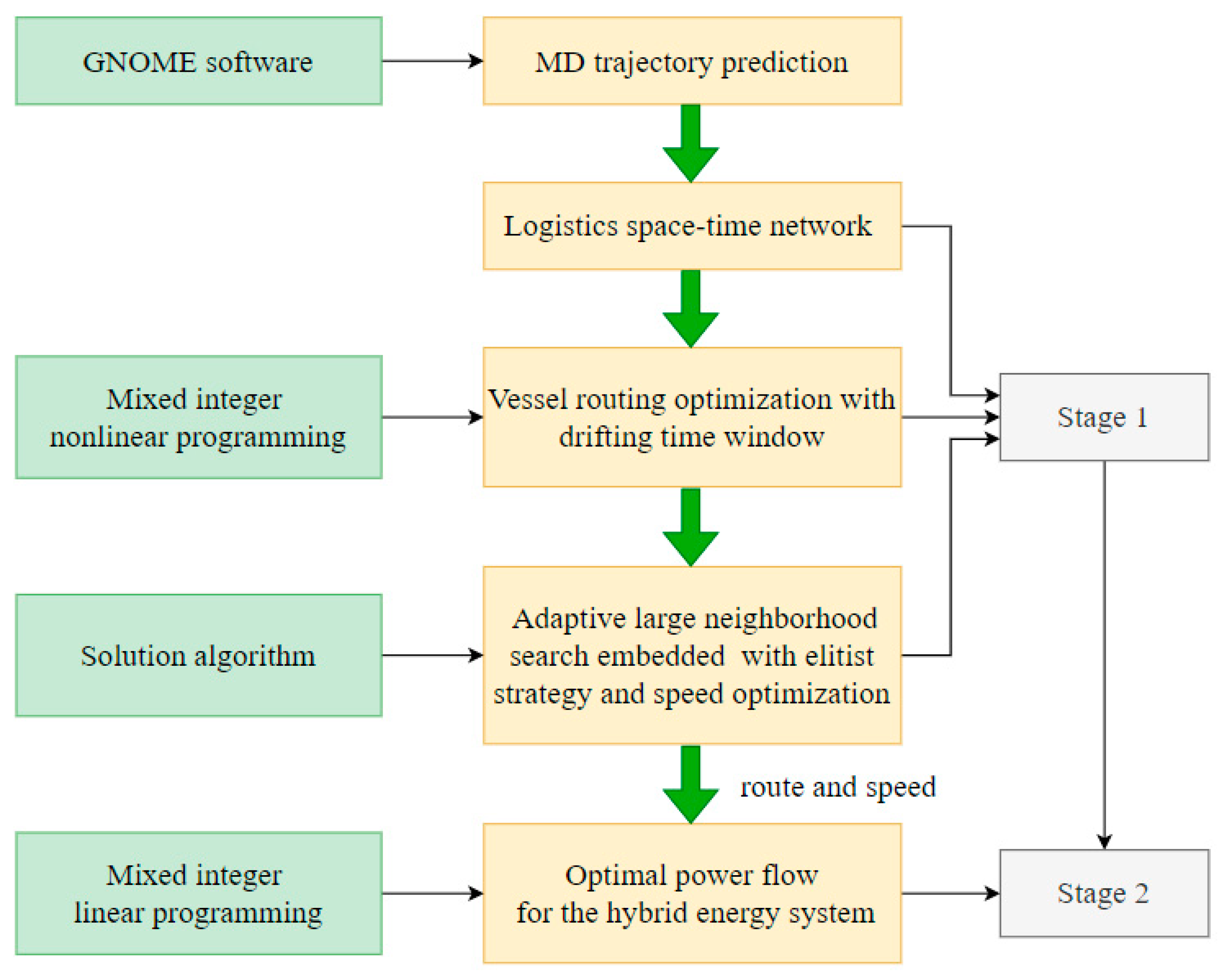
3. Two-Stage Optimization Approach
3.1. Problem Description
3.2. First Stage
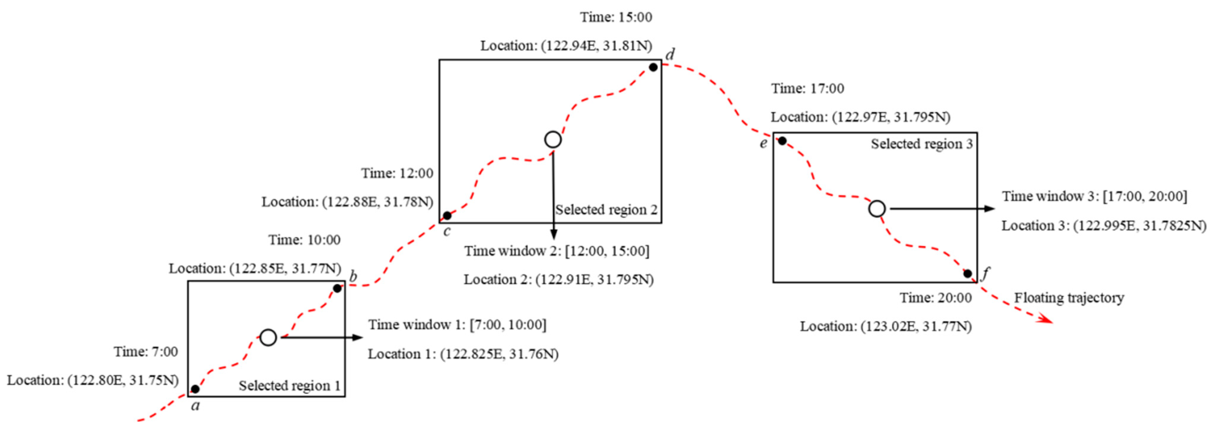
3.2.1. Drifting Time Window
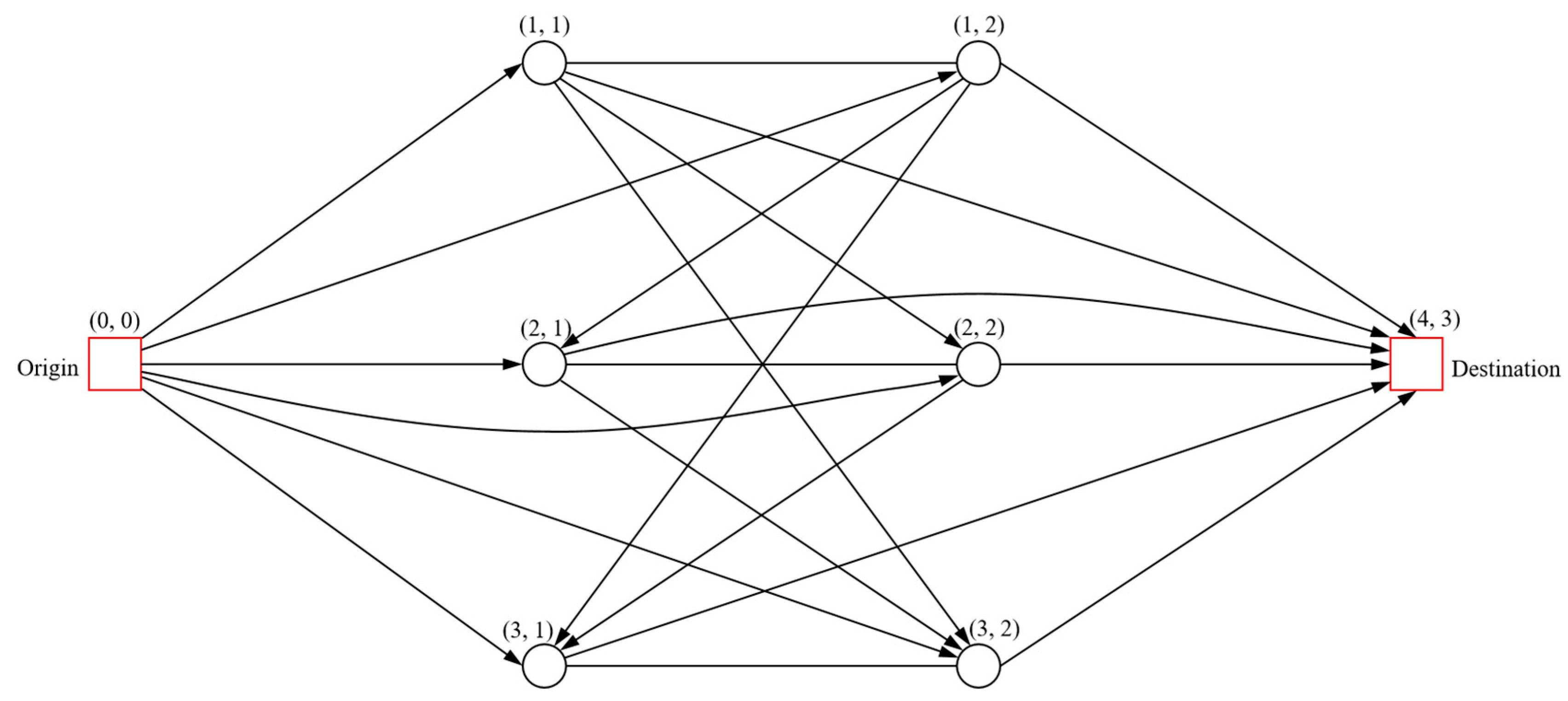
3.2.2. Logistics Space–Time Network
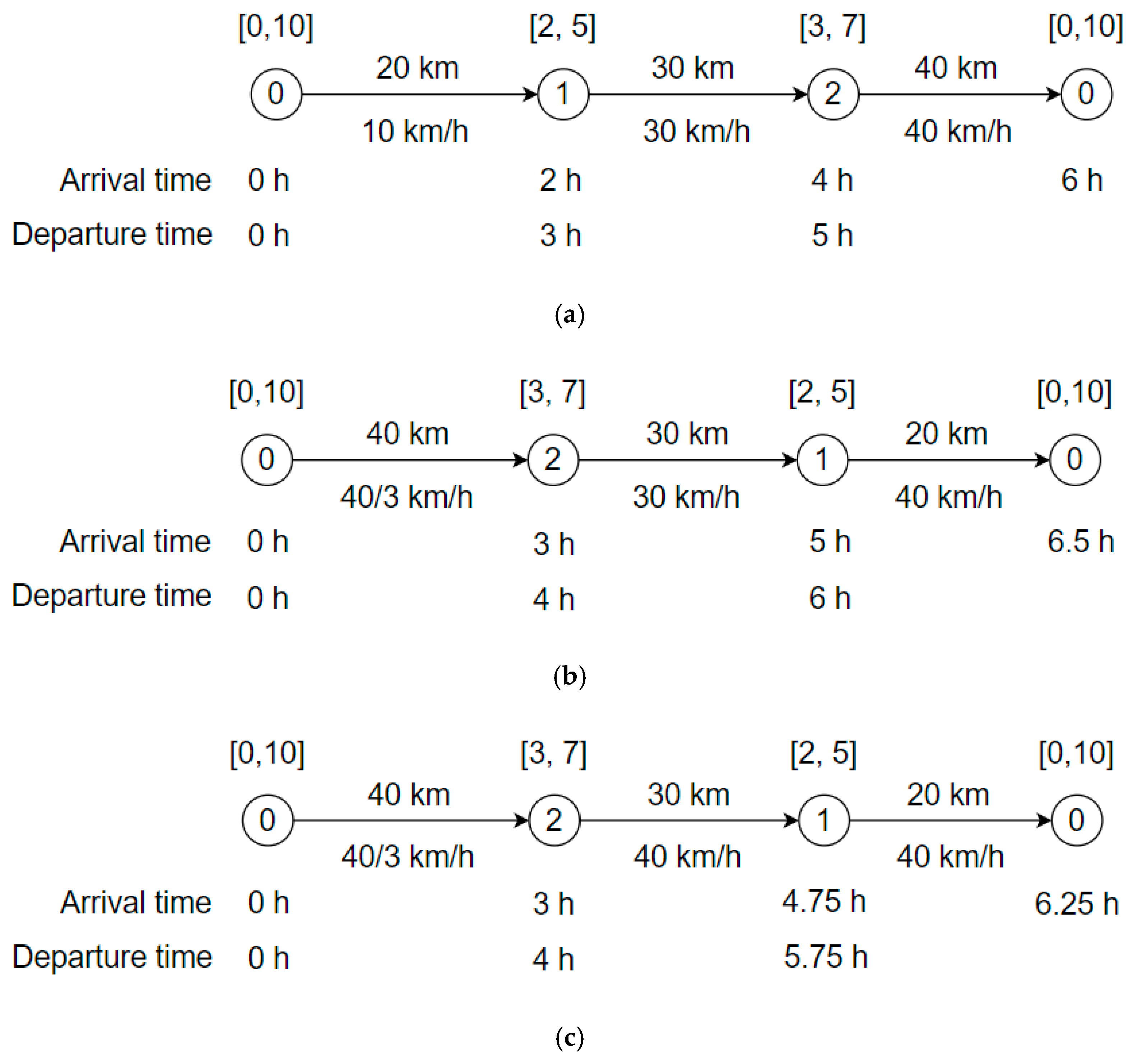
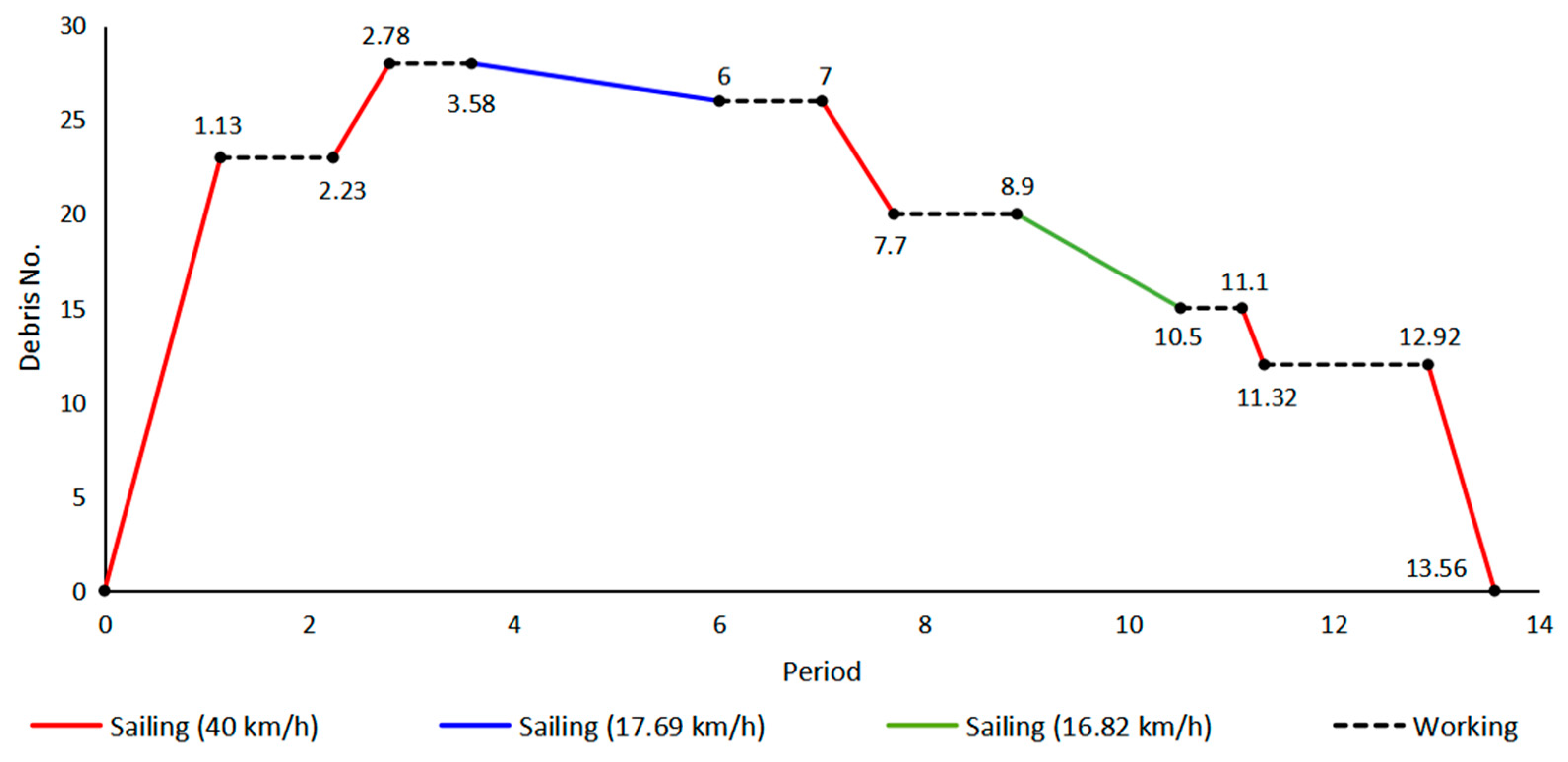
3.2.3. VRPDTW and Speed Optimization Model
3.3. Second Stage
3.3.1. Power Demand
3.3.2. PV Output
3.3.3. OPF Model
4. Solution Algorithm for VRPDTW
4.1. Removal Operators
4.2. Insertion Operators
4.3. Speed Optimization
4.4. Adaptive Operator Selection Mechanism
4.4.1. Selection Probability
4.4.2. Operator Score
4.4.3. Elitist Strategy
| Algorithm 1 ALNSES algorithm |
|
| Generate an initial feasible solutions population Find the best solution |
Initialize and |
| while |
| for |
| Select removal operator and insertion operator according to and , respectively |
| Perform operators and on a feasible solution to obtain |
| Perform SO algorithm on to obtain |
| if |
| if |
| else |
| end |
| else |
| end |
| if mod = 0 |
| Update and according to Equation (46) |
| Update and according to Equation (47) |
| end |
| end |
| Merge parent population and offspring population to obtain population |
| Update population : Perform Elite strategy on to obtain new parent population |
| end |
5. Numerical Experiment
5.1. Experiment Data
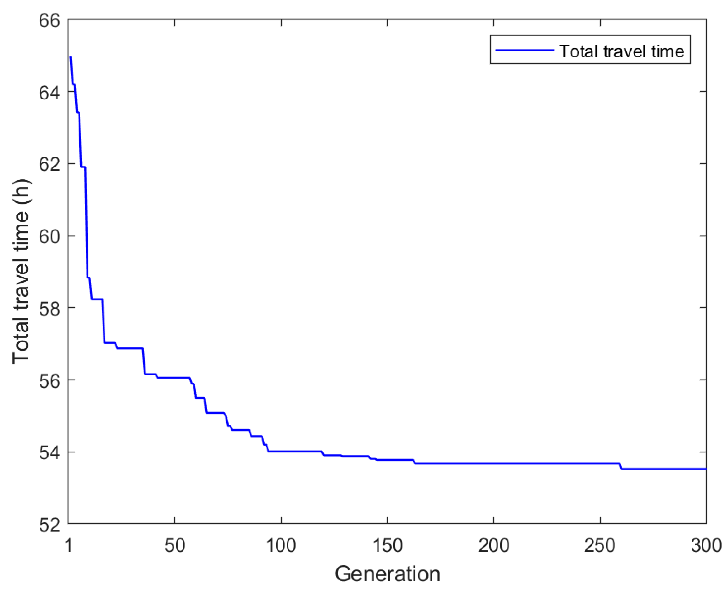
5.2. Algorithm Performance
5.3. HES
5.3.1. Data
- Scenario A: maximum likely output. In the historical data greater than the most likely one, the illumination intensity that occurs the most is selected, and the PV output calculated from this is the maximum likely output.
- Scenario B: most likely output. In all historical data, the illumination intensity with the highest occurrence is taken as the most likely one, and the PV output calculated is thus regarded as the most likely output. This scenario is used as the baseline for further analysis.
- Scenario C: minimum likely output. In the historical data less than the most likely one, the illumination intensity with the most occurrence times is selected, and the PV output calculated from this is the minimum possible PV output.
5.3.2. OPF Analysis
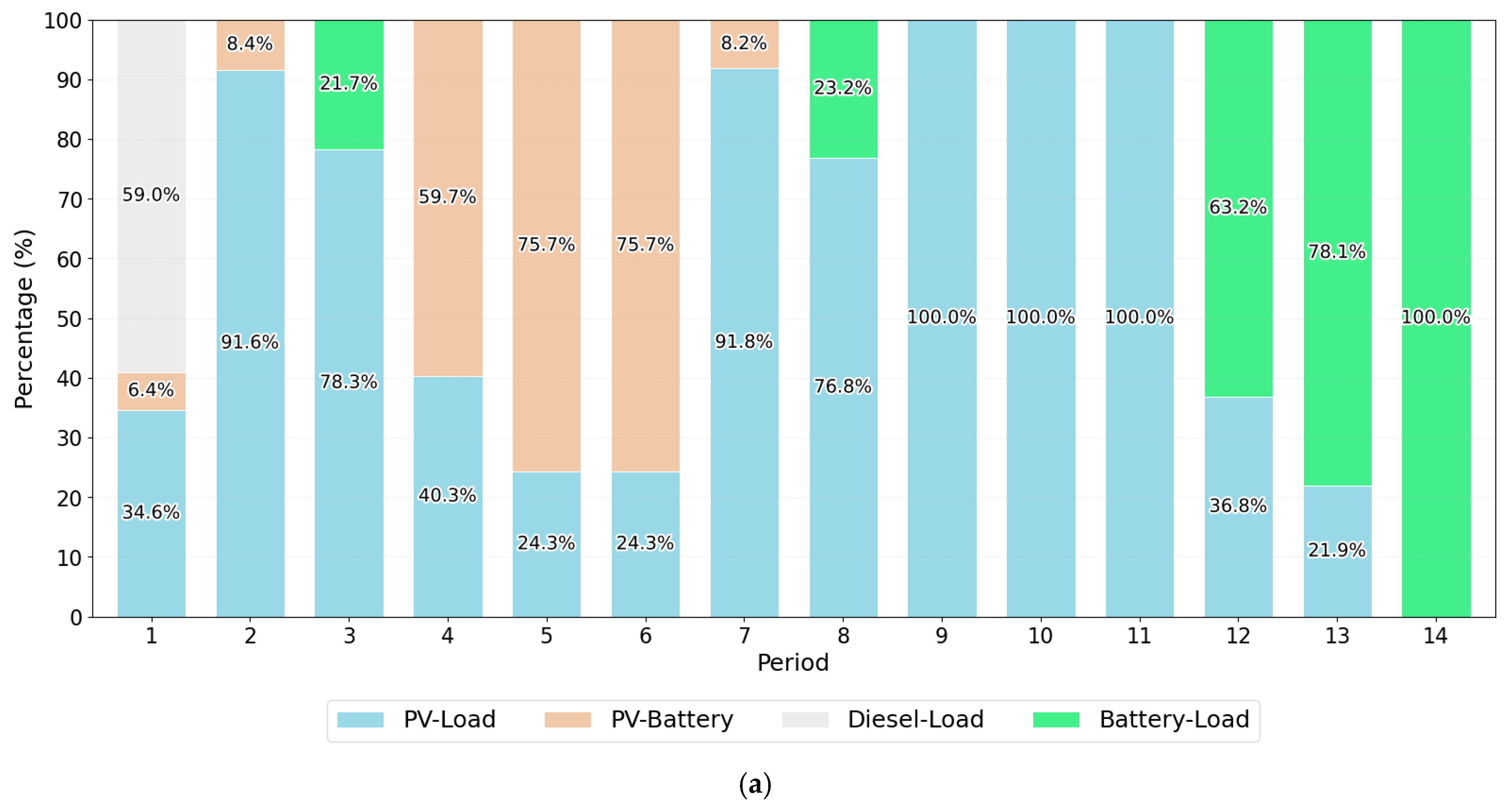
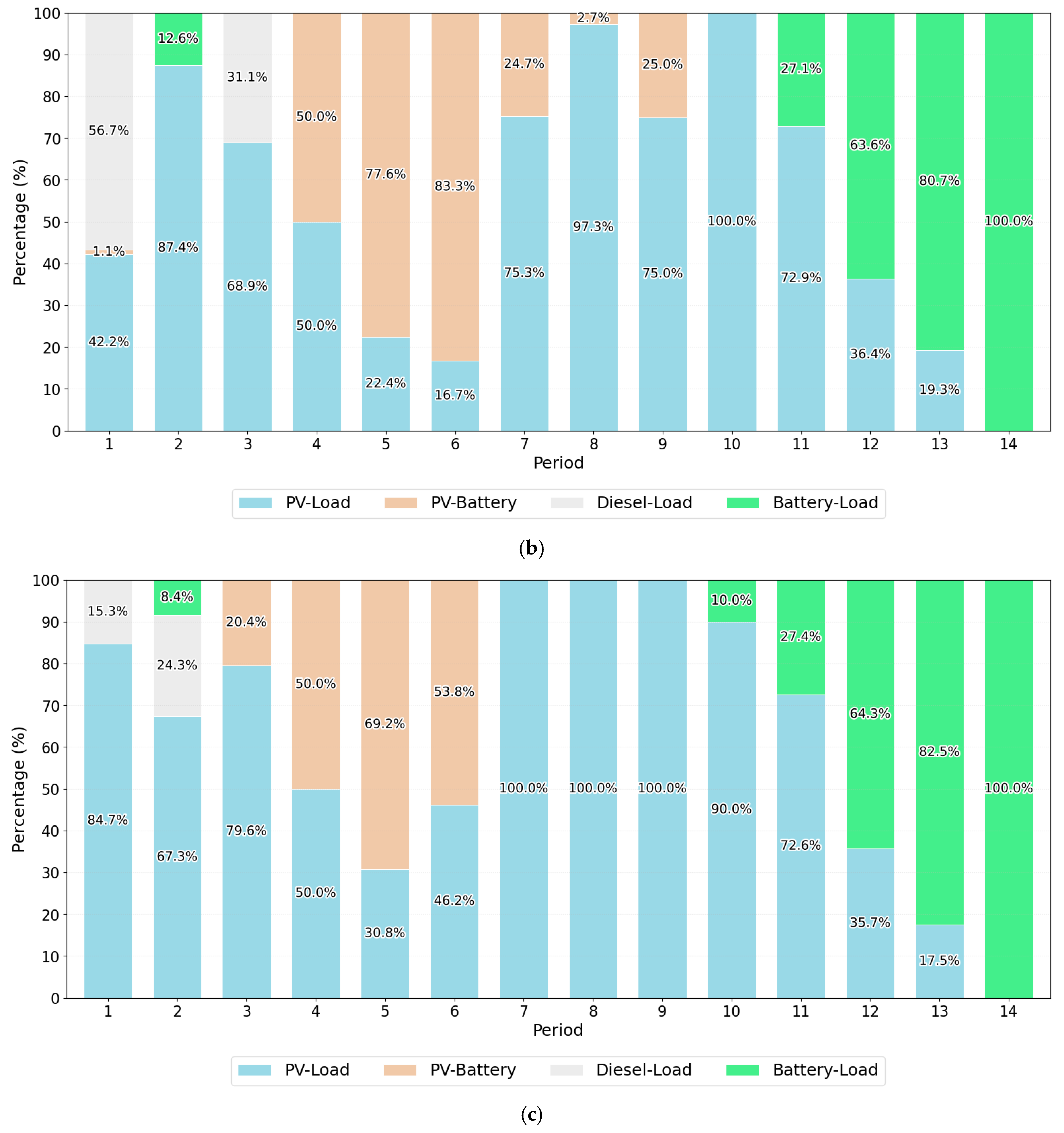
- The reason there is no Diesel-Battery in the OPF is that the cost of the battery powering load after diesel has charged the battery is higher than if diesel powers the load directly. Thus, to save costs, diesel does not charge the battery.
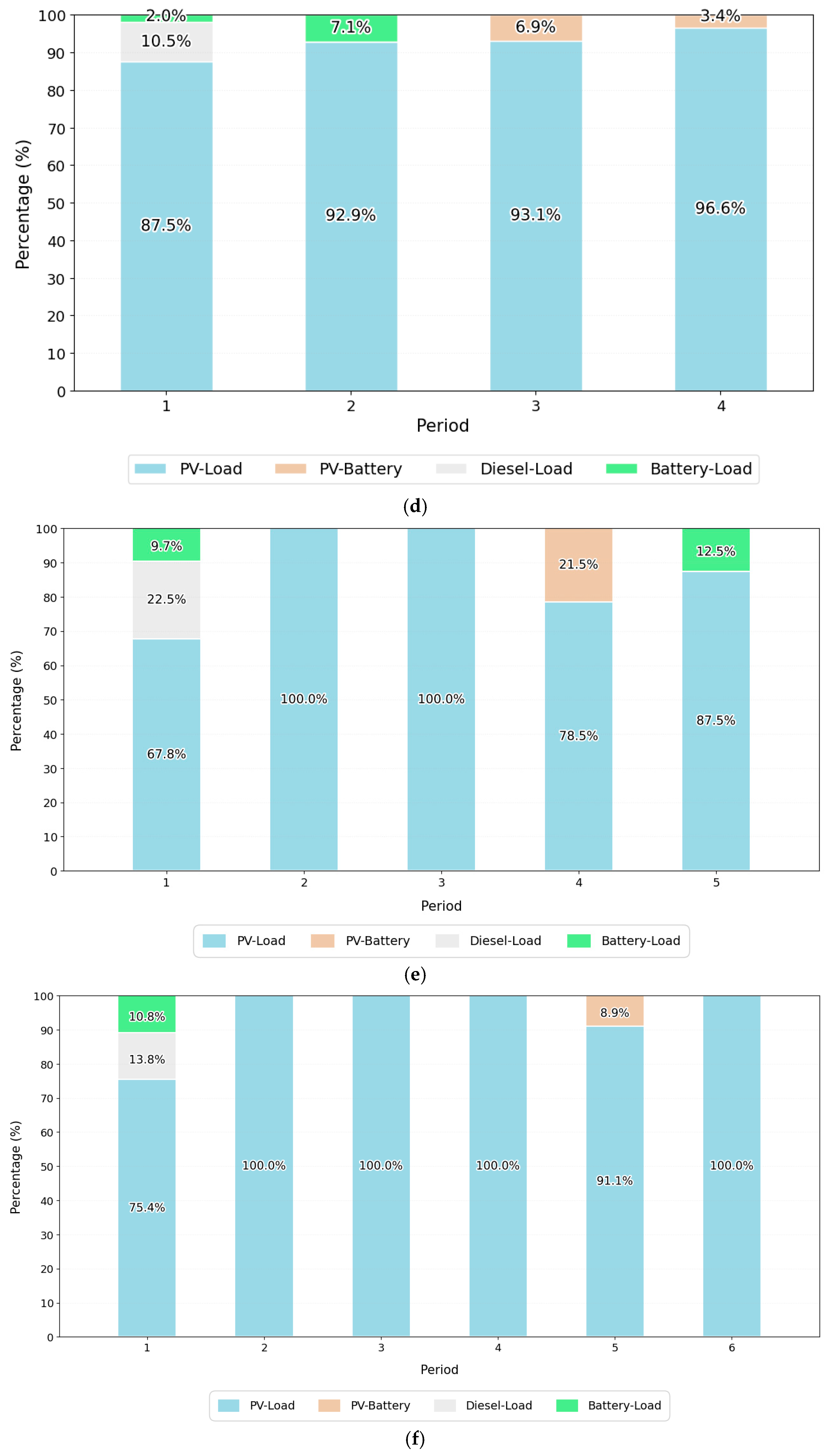
- According to the length of the travel time, all vessels can be divided into two categories, the first three vessels with 14 periods (Category 1) and the last three vessels with no more than 6 periods (Category 2). On the one hand, the two categories share some characteristics. (1) There is no separate output of diesel at any period; (2) there are only three kinds of energy output at most, i.e., Diesel-Load, PV-Load, and PV-Battery, which only occurs in the first two periods; (3) PV-Battery and Battery-Load do not occur in the same period; and (4) PV-Battery must occur simultaneously with PV-Load, which indicates that the condition for PV to charge the battery is when PV supplies power to the load and there is surplus. On the other hand, each category presents different characteristics.
- In Category 1, due to the long trip, PV-Battery and Battery-Load have more outputs except PV-Load. PV-Load runs through almost all of the periods except the last period where the load is completely powered by battery. It is easy to see from Table 14 that PV output in the last period is 0. Diesel-Load occurs in the first three periods, ranging from 15.33% to 59.03%. PV-Battery appears in the front and middle periods (from 1 to 9), reaching a maximum of 83.31%. Battery-Load is mainly located in the later period (from 10 to 14), and the later the period, the higher the proportion.
- In Category 2, the short-trip results in the load being mostly supplied by PV, and the other energy outputs are extremely low. Diesel-Load only appears in period 1, ranging from 3.45% to 21.46%. PV-Battery and Battery-Load are, respectively, no more than 22% and 13% in each period.
5.3.3. Carbon Emissions
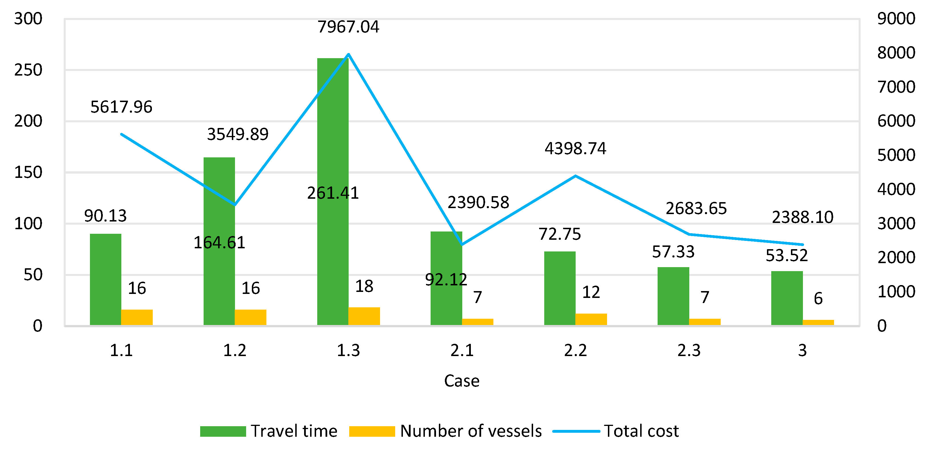
5.4. Time Windows
6. Conclusions
Author Contributions
Funding
Institutional Review Board Statement
Informed Consent Statement
Data Availability Statement
Conflicts of Interest
Abbreviations
| ALNS | Adaptive Large Neighborhood Search |
| ALNSES | ALNS embedded with Elitist Strategy |
| ECA | Emission Control Areas |
| EMS | Energy Management Strategies |
| GNOME | General NOAA Operational Modeling Environment |
| HES | Hybrid Energy System |
| MD | Marine Debris |
| MDL | MD Location |
| MILP | Mixed Integer Linear Programming |
| NOAA | National Oceanic and Atmospheric Administration |
| OPF | Optimal Power Flow |
| PV | Photovoltaic |
| SOA | Speed Optimization Algorithm |
| SOC | State of Charge |
| VRP | Vessel Routing Problem |
| VRPDTW | VRP with Drifting Time Window |
Appendix A
Speed Optimization Algorithm
| Algorithm A1 Speed optimization algorithm |
| Input: . Output: Speed vector . for if else if end end end |
References
- Beaumont, N.J.; Aanesen, M.; Austen, M.C.; Börger, T.; Clark, J.R.; Cole, M.; Hooper, T.; Lindeque, P.K.; Pascoe, C.; Wyles, K.J. Global ecological, social and economic impacts of marine plastic. Mar. Pollut. Bull. 2019, 142, 189–195. [Google Scholar] [CrossRef] [PubMed]
- McGlade, J. From Pollution to Solution: A Global Assessment of Marine Litter and Plastic Pollution. United Nations Environment Programme Report. 2021. Available online: https://nottingham-repository.worktribe.com/output/8047115 (accessed on 10 January 2022).
- Yaghmour, F.; Samara, F.; Ghalayini, T.; Kanan, S.M.; Elsayed, Y.; Bousi, M.A.; Naqbi, H.A. Junk food: Polymer composition of macroplastic marine debris ingested by green and loggerhead sea turtles from the Gulf of Oman. Sci. Total Environ. 2022, 828, 154373. [Google Scholar] [CrossRef] [PubMed]
- Costa, R.; Sá, S.; Pereira, A.T.; Ângelo, A.R.; Vaqueiro, J.; Ferreira, M.; Eira, C. Prevalence of entanglements of seabirds in marine debris in the central Portuguese coast. Mar. Pollut. Bull. 2020, 161, 111746. [Google Scholar] [CrossRef]
- Kuzin, A.; Trukhin, A. Entanglement of Steller sea lions (Eumetopias jubatus) in man-made marine debris on Tyuleniy Island, Sea of Okhotsk. Mar. Pollut. Bull. 2022, 177, 113521. [Google Scholar] [CrossRef]
- Prestholdt, T.; Kemp, L. The effects of anthropogenic marine debris on the behavior of the purple shore crab, Hemigrapsus nudus. J. Sea Res. 2020, 163, 101916. [Google Scholar] [CrossRef]
- Eisfeld-Pierantonio, S.; Pierantonio, N.; Simmonds, M. The impact of marine debris on cetaceans with consideration of plastics generated by the COVID-19 pandemic. Environ. Pollut. 2022, 300, 118967. [Google Scholar] [CrossRef]
- Casabianca, S.; Bellingeri, A.; Capellacci, S.; Sbrana, A.; Russo, T.; Corsi, I.; Penna, A. Ecological implications beyond the ecotoxicity of plastic debris on marine phytoplankton assemblage structure and functioning. Environ. Pollut. 2021, 290, 118101. [Google Scholar] [CrossRef] [PubMed]
- Löhr, A.; Savelli, H.; Beunen, R.; Kalz, M.; Ragas, A.; Belleghem, F.V. Solutions for global marine litter pollution. Curr. Opin. Environ. Sustain. 2017, 28, 90–99. [Google Scholar] [CrossRef]
- Rochman, C.; Tahir, A.; Williams, S.; Baxa, D.V.; Lam, R.; Miller, J.T.; Teh, F.; Werorilangi, S.; Teh, S.J. Anthropogenic debris in seafood: Plastic debris and fibers from textiles in fish and bivalves sold for human consumption. Sci. Rep. 2015, 5, 14340. [Google Scholar] [CrossRef]
- Duan, G.; Aghalari, A.; Chen, L.; Marufuzzaman, M.; Ma, J. Vessel routing optimization for floating macro-marine debris collection in the ocean considering dynamic velocity and direction. Transp. Res. E 2021, 152, 102414. [Google Scholar] [CrossRef]
- Duan, G.; Zhang, K. Optimization on hybrid energy vessel routing and energy management for floating marine debris cleanup. Transport. Res. C 2022, 138, 103649. [Google Scholar] [CrossRef]
- Yuan, Y.; Wang, J.; Yan, X.; Shen, B.; Long, T. A review of multi-energy hybrid power system for ships. Renew. Sustain. Energy Rev. 2020, 132, 110081. [Google Scholar] [CrossRef]
- Duan, G.; Nur, F.; Alizadeh, M.; Chen, L.; Marufuzzaman, M.; Ma, J. Vessel routing and optimization for marine debris collection with consideration of carbon cap. J. Clean. Prod. 2020, 263, 121399. [Google Scholar] [CrossRef]
- Park, C.; Jeong, B.; Zhou, P.; Jang, H.; Kim, S.; Jeon, H.; Nam, D.; Rashedi, A. Live-Life cycle assessment of the electric propulsion ship using solar PV. Appl. Energy 2022, 309, 118477. [Google Scholar] [CrossRef]
- Lan, H.; Wen, S.; Hong, Y.; Yu, D.C.; Zhang, L. Optimal sizing of hybrid PV/diesel/battery in ship power system. Appl. Energy 2015, 158, 26–34. [Google Scholar] [CrossRef]
- Sui, Q.; Zhang, R.; Wu, C.; Wei, F.; Lin, X.; Li, Z. Stochastic scheduling of an electric vessel-based energy management system in pelagic clustering islands. Appl. Energy 2020, 259, 114155. [Google Scholar] [CrossRef]
- Gkerekos, C.; Lazakis, I. A novel, data-driven heuristic framework for vessel weather routing. Ocean Eng. 2020, 197, 106887. [Google Scholar] [CrossRef]
- Wei, Z.; Zhao, L.; Zhang, X.; Lv, W. Jointly optimizing ocean shipping routes and sailing speed while considering involuntary and voluntary speed loss. Ocean Eng. 2022, 245, 110460. [Google Scholar] [CrossRef]
- Zis, T.; Psaraftis, H.; Ding, L. Ship weather routing: A taxonomy and survey. Ocean Eng. 2020, 213, 107697. [Google Scholar] [CrossRef]
- Weng, J.; Han, T.; Shi, K.; Li, G. Impact analysis of ECA policies on ship trajectories and emissions. Mar. Pollut. Bull. 2022, 179, 113687. [Google Scholar] [CrossRef]
- Ma, D.; Ma, W.; Jin, S.; Ma, X. Method for simultaneously optimizing ship route and speed with emission control areas. Ocean Eng. 2020, 202, 107170. [Google Scholar] [CrossRef]
- Li, L.; Gao, S.; Yang, W.; Xiong, X. Ship’s response strategy to emission control areas: From the perspective of sailing pattern optimization and evasion strategy selection. Transport. Res. E 2020, 133, 101835. [Google Scholar] [CrossRef]
- Ma, W.; Ma, D.; Ma, Y.; Zhang, J.; Wang, D. Green maritime: A routing and speed multi-objective optimization strategy. J. Clean. Prod. 2021, 305, 127179. [Google Scholar] [CrossRef]
- Ghenai, C.; Bettayeb, M.; Brdjanin, B.; Hamid, A.K. Hybrid solar PV/PEM fuel Cell/Diesel Generator power system for cruise ship: A case study in Stockholm, Sweden. Case Stud. Therm. Eng. 2019, 14, 100497. [Google Scholar] [CrossRef]
- Ballini, F.; Ölçer, A.I.; Brandt, J.; Neumann, D. Health costs and economic impact of wind assisted ship propulsion. Ocean Eng. 2017, 146, 477–485. [Google Scholar] [CrossRef]
- Pan, P.; Sun, Y.; Yuan, C.; Yan, X.; Tang, X. Research progress on ship power systems integrated with new energy sources: A review. Renew. Sustain. Energy Rev. 2021, 144, 111048. [Google Scholar] [CrossRef]
- Wen, S.; Lan, H.; YU, D.; Fu, Q.; Hong, Y.; Yu, L.; Yang, R. Optimal sizing of hybrid energy storage sub-systems in PV/diesel ship power system using frequency analysis. Energy 2017, 140, 198–208. [Google Scholar] [CrossRef]
- Tang, R.; Li, X.; Lai, J. A novel optimal energy-management strategy for a maritime hybrid energy system based on large-scale global optimization. Appl. Energy 2018, 228, 254–264. [Google Scholar] [CrossRef]
- Haseltalab, A.; Biert, L.V.; Sapra, H.; Mestemaker, B.; Negenborn, R.R. Component sizing and energy management for SOFC-based ship power systems. Energy Convers. Manag. 2021, 245, 114625. [Google Scholar] [CrossRef]
- Chen, H.; Zhang, Z.; Guan, C.; Gao, H. Optimization of sizing and frequency control in battery/supercapacitor hybrid energy storage system for fuel cell ship. Energy 2020, 197, 117285. [Google Scholar] [CrossRef]
- Ma, L.; Yang, P.; Gao, D.; Bao, C. A multi-objective energy efficiency optimization method of ship under different sea conditions. Ocean. Eng. 2023, 290, 116337. [Google Scholar] [CrossRef]
- Öztürk, O.; Başar, E. Multiple linear regression analysis and artificial neural networks based decision support system for energy efficiency in shipping. Ocean. Eng. 2022, 243, 110209. [Google Scholar] [CrossRef]
- Koumaniotis, E.K.; Kanellos, F.D. Optimal routing and sustainable operation scheduling of large ships with integrated full-electric propulsion. Sustainability 2024, 16, 10662. [Google Scholar] [CrossRef]
- Zhu, J.; Shen, H.; Tang, Q.; Qin, Z.; Yu, Y. Energy-efficient route planning method for ships based on level set. Sensors 2025, 25, 381. [Google Scholar] [CrossRef] [PubMed]
- Pan, X.; Zhu, X.; Zhao, F. More environmental sustainability routing and energy management for all electric ships. Front. Energy Res. 2022, 9, 821236. [Google Scholar] [CrossRef]
- Duan, G.; Fan, T.; Chen, L.; Ma, J. Floating marine debris mitigation by vessel routing modeling and optimization considering carbon emission and travel time. Transport. Res. C 2021, 133, 103449. [Google Scholar] [CrossRef]
- Maximenko, N.; Hafner, J.; Kamachi, M.; MacFadyen, A. Numerical simulations of debris drift from the Great Japan Tsunami of 2011 and their verification with observational reports. Mar. Pollut. Bull. 2018, 132, 5–25. [Google Scholar] [CrossRef]
- Purba, N.P.; Faizal, I.; Cordova, M.R.; Abimanyu, A.; Afandi, N.K.; Indriawan, D.; Khan, A.M. Marine Debris Pathway Across Indonesian Boundary Seas. J. Ecol. Eng. 2021, 22, 82–98. [Google Scholar] [CrossRef]
- Ropke, S.; Pisinger, D. An adaptive large neighborhood search heuristic for the pickup and delivery problem with time windows. Transport. Sci. 2006, 40, 455–472. [Google Scholar] [CrossRef]
- Hasani, A.; Khosrojerdi, A. Robust global supply chain network design under disruption and uncertainty considering resilience strategies: A parallel memetic algorithm for a real-life case study. Transport. Res. E 2016, 87, 20–52. [Google Scholar] [CrossRef]
- Koç, Ç.; Bektaş, T.; Jabali, O.; Laporte, G. The impact of depot location, fleet composition and routing on emissions in city logistics. Transport. Res. B 2016, 84, 81–102. [Google Scholar] [CrossRef]
- Hiermann, G.; Puchinger, J.; Ropke, S.; Hartl, R.F. The Electric Fleet Size and Mix Vehicle Routing Problem with Time Windows and Recharging Stations. Eur. J. Oper. Res. 2016, 252, 995–1018. [Google Scholar] [CrossRef]
- Mara, S.; Norcahyo, R.; Jodiawan, P.; Lusiantoro, L.; Rifai, A.P. A survey of adaptive large neighborhood search algorithms and applications. Comput. Oper. Res. 2022, 146, 105903. [Google Scholar] [CrossRef]
- Emilsson, E.; Dahllf, L. Lithium-Ion Vehicle Battery Production—Status 2019 on Energy Use, CO2 Emissions, Use of Metals, Products Environmental Footprint, and Recycling; IVL Swedish Environmental Research Institute: Stockholm, Sweden, 2019. [Google Scholar]
- Cheng, D. Carbon Emissions Calculation of Gasoline and Diesel Fuel Based on Life Cycle Assessment; China University of Petroleum: Beijing, China, 2016. [Google Scholar]


| Sets: | ||
|---|---|---|
| Set of time window for origin, | ||
| Set of time windows of MDs, | ||
| Set of time window for destination, | ||
| Set of all vertices, | ||
| Set of origin, | ||
| Set of MDs, | ||
| Set of destination, | ||
| Set of edges, | ||
| Set of origin with time window, | ||
| Set of MDLs, | ||
| Set of destination with time window, | ||
| Set of all edges, | ||
| Set of edges from origin with time window to an MDL, | ||
| Set of edges from one MDL to another, | ||
| Set of edges from an MDL to destination with time window, | ||
| Set of vessels | ||
| Parameters: | ||
| MD collection time at vertex | ||
| MD volume at vertex | ||
| MD density at vertex | ||
| Time window of vertex , and are the earliest time and the latest time, respectively | ||
| Maximum design speed of the vessel | ||
| Weight capacity of vessel | ||
| Volume capacity of vessel | ||
| Distance of edge | ||
| Decision variables: | ||
| 1 if vessel transfers edge ; 0 otherwise | ||
| Cumulative loaded volume of vessel at vertex | ||
| Cumulative loaded weight of vessel at vertex | ||
| The speed of vessel on edge | ||
| Arrival time of vessel at vertex | ||
| Set: | |
|---|---|
| Set of all periods, | |
| Parameters: | |
| Loss cost of PV power generation | |
| Cost of diesel | |
| Loss cost of battery charging and discharging | |
| Carbon tax rate | |
| Carbon emission factor | |
| Diesel intercept coefficient | |
| Diesel slope coefficient | |
| Power required for load of vessel in period | |
| Maximum output power of PV in period | |
| Battery charging efficiency | |
| Battery discharge efficiency | |
| Maximum value of battery SOC | |
| Minimum value of battery SOC | |
| Rated power of PV power | |
| Rated power of diesel generator | |
| Maximum power of PV to vessel load | |
| Maximum power of PV to battery | |
| Maximum power of diesel generator to vessel load | |
| Maximum power of diesel generator to battery | |
| Maximum power of storage battery to vessel load | |
| Decision Variables: | |
| Power of PV to load of vessel in period | |
| Power of PV to battery of vessel in period | |
| Power of diesel generator to load of vessel in period | |
| Power of diesel generator to battery in period | |
| Power of storage battery to load of vessel in period | |
| Battery SOC of vessel at the beginning of period | |
| 1 if the battery of vessel is charged in period ; 0 otherwise | |
| 1 if the battery of vessel is discharged in period ; 0 otherwise | |
| 1 if the diesel generator of vessel is on in period ; 0 otherwise | |
| Debris No. | 1 | 2 | 3 | 4 | 5 | 6 | 7 | 8 | 9 | 10 |
| Weight (tons) | 1.91 | 2.16 | 2.55 | 1.27 | 1.59 | 1.01 | 1.13 | 2.07 | 1.37 | 2.64 |
| Volume (m3) | 2.67 | 2.81 | 3.57 | 1.78 | 1.91 | 1.31 | 1.69 | 2.48 | 1.92 | 3.17 |
| Collection time (h) | 1.1 | 1.1 | 1.5 | 0.9 | 0.9 | 0.8 | 0.9 | 1.0 | 0.9 | 1.3 |
| Debris No. | 11 | 12 | 13 | 14 | 15 | 16 | 17 | 18 | 19 | 20 |
| Weight (tons) | 2.15 | 2.52 | 1.24 | 1.87 | 0.53 | 0.71 | 2.92 | 2.09 | 0.97 | 2.07 |
| Volume (m3) | 2.80 | 3.78 | 1.86 | 2.81 | 0.69 | 0.92 | 3.8 | 2.51 | 1.26 | 3.1 |
| Collection time (h) | 1.1 | 1.6 | 0.9 | 1.1 | 0.6 | 0.9 | 1.6 | 1.0 | 0.8 | 1.2 |
| Debris No. | 21 | 22 | 23 | 24 | 25 | 26 | 27 | 28 | 29 | 30 |
| Weight (tons) | 2.67 | 1.09 | 1.91 | 1.60 | 0.33 | 1.83 | 1.01 | 1.12 | 0.66 | 2.87 |
| Volume (m3) | 3.47 | 1.31 | 2.87 | 2.24 | 0.39 | 2.38 | 1.31 | 1.35 | 0.98 | 3.45 |
| Collection time (h) | 1.5 | 0.8 | 1.1 | 1.0 | 0.5 | 1.0 | 0.8 | 0.8 | 0.7 | 1.4 |
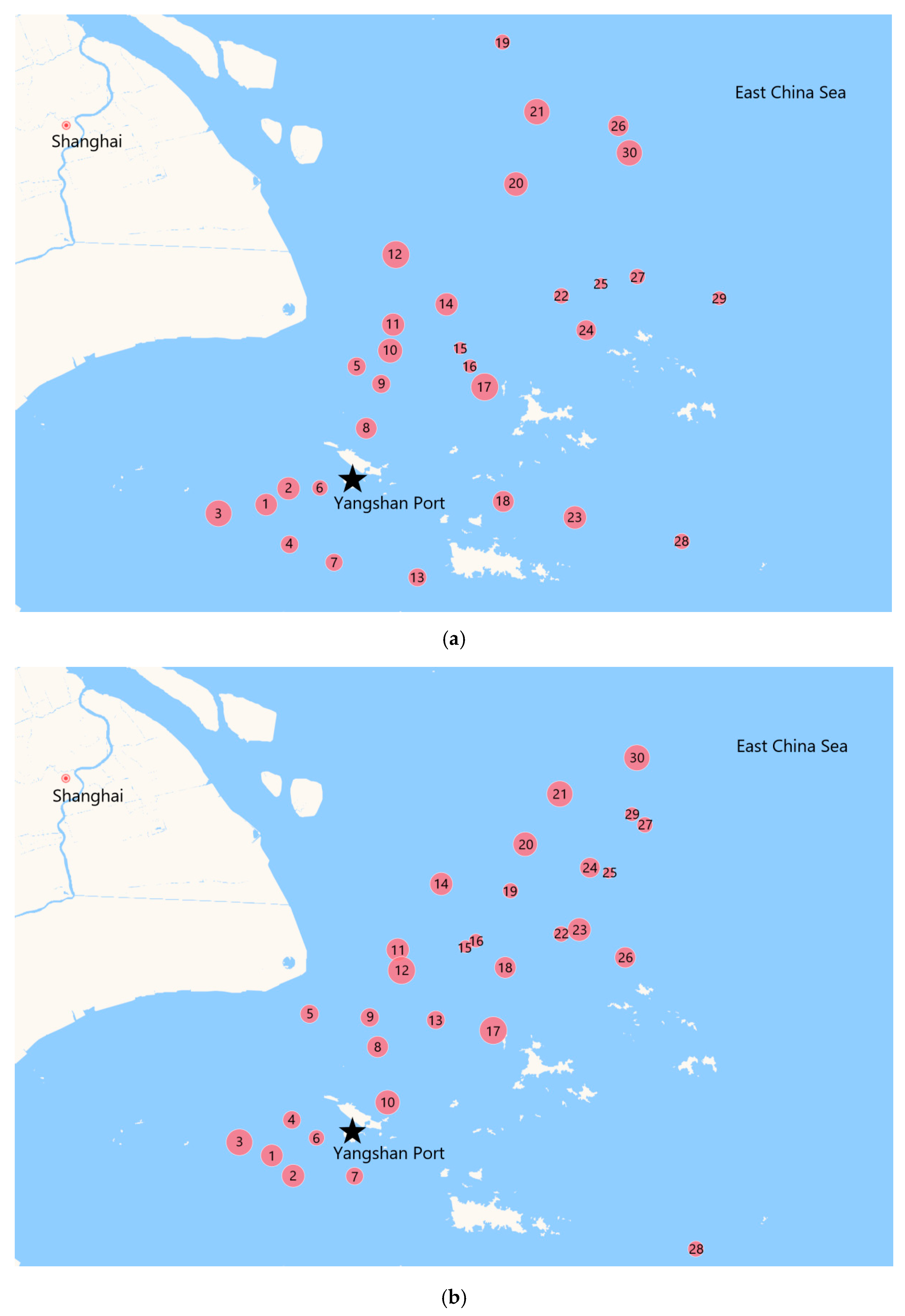
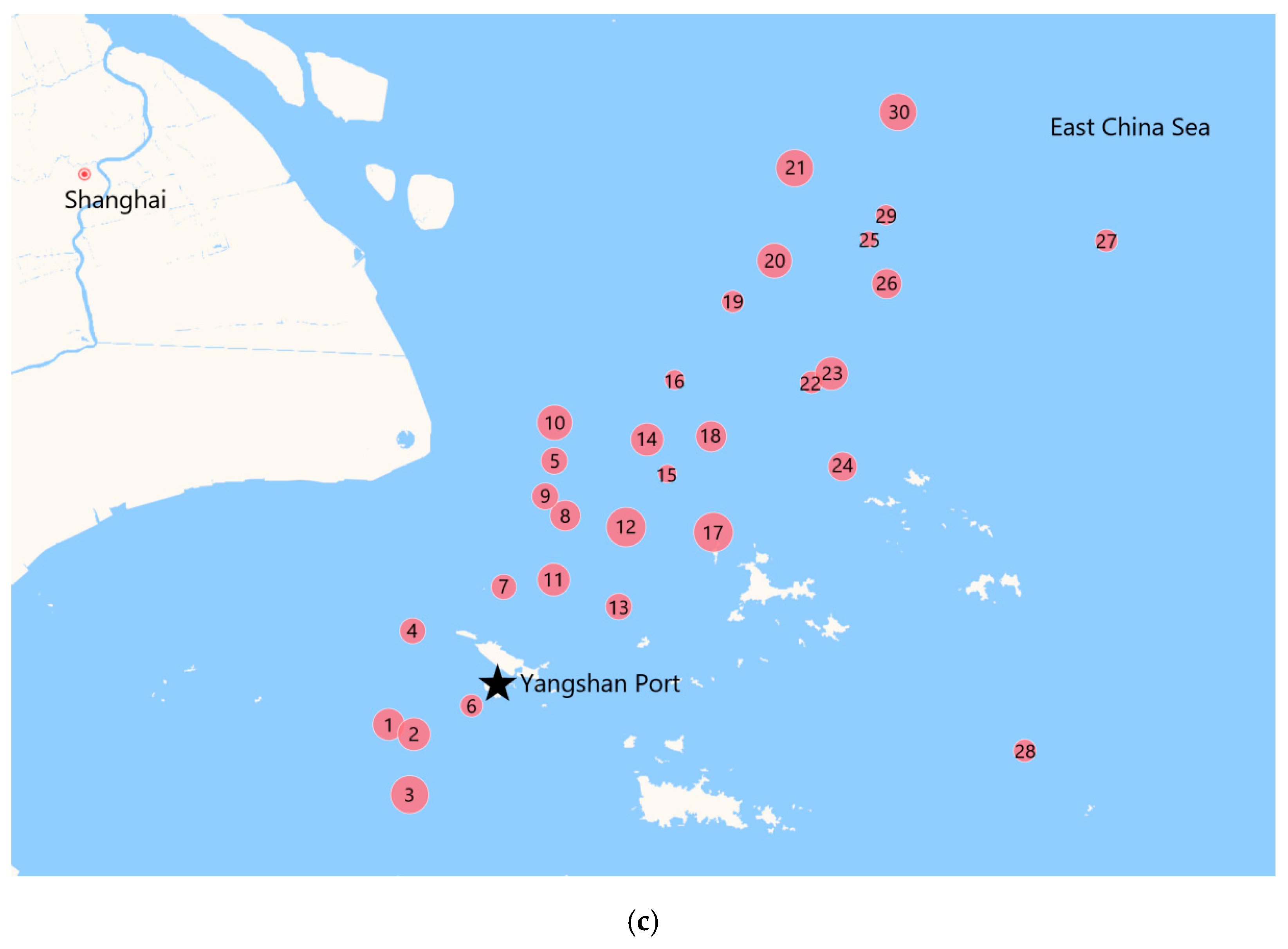
| Time Window | [7, 10] | [13, 15] | [17.5, 19.5] | |||
|---|---|---|---|---|---|---|
| Debris No. | Latitude | Longitude | Latitude | Longitude | Latitude | Longitude |
| 0 | 30.5922 | 122.0746 | 30.5922 | 122.0746 | 30.5922 | 122.0746 |
| 1 | 30.5443 | 121.8925 | 30.5497 | 121.9043 | 30.5403 | 121.9154 |
| 2 | 30.5735 | 121.9392 | 30.5130 | 121.9491 | 30.5280 | 121.9523 |
| 3 | 30.5284 | 121.7923 | 30.5736 | 121.8362 | 30.4521 | 121.9460 |
| 4 | 30.4722 | 121.9415 | 30.6140 | 121.9462 | 30.6576 | 121.9503 |
| 5 | 30.7940 | 122.0825 | 30.8051 | 121.9833 | 30.8706 | 122.1567 |
| 6 | 30.5745 | 122.0054 | 30.5816 | 121.9981 | 30.5639 | 122.0362 |
| 7 | 30.4397 | 122.0351 | 30.5124 | 122.0778 | 30.7127 | 122.0831 |
| 8 | 30.6824 | 122.1027 | 30.7435 | 122.1245 | 30.8020 | 122.1727 |
| 9 | 30.7625 | 122.1340 | 30.7987 | 122.1095 | 30.8261 | 122.1435 |
| 10 | 30.8226 | 122.1530 | 30.6455 | 122.1468 | 30.9182 | 122.1572 |
| 11 | 30.8695 | 122.1593 | 30.9207 | 122.1681 | 30.7218 | 122.1558 |
| 12 | 30.9958 | 122.1649 | 30.8834 | 122.1763 | 30.7876 | 122.2613 |
| 13 | 30.4125 | 122.2102 | 30.7941 | 122.2481 | 30.6881 | 122.2506 |
| 14 | 30.9061 | 122.2715 | 31.0390 | 122.2595 | 30.8971 | 122.2920 |
| 15 | 30.8272 | 122.3001 | 30.9263 | 122.3102 | 30.8544 | 122.3215 |
| 16 | 30.7945 | 122.3210 | 30.9369 | 122.3321 | 30.9719 | 122.3321 |
| 17 | 30.7571 | 122.3516 | 30.7753 | 122.3685 | 30.7811 | 122.3885 |
| 18 | 30.5500 | 122.3907 | 30.8887 | 122.3936 | 30.9011 | 122.3853 |
| 19 | 31.3781 | 122.3890 | 31.0267 | 122.4047 | 31.0695 | 122.4168 |
| 20 | 31.1228 | 122.4172 | 31.1103 | 122.4354 | 31.1205 | 122.4775 |
| 21 | 31.2529 | 122.4611 | 31.2005 | 122.5079 | 31.2359 | 122.5070 |
| 22 | 30.9215 | 122.5127 | 30.9489 | 122.5108 | 30.9687 | 122.5315 |
| 23 | 30.5210 | 122.5411 | 30.9569 | 122.5488 | 30.9795 | 122.5605 |
| 24 | 30.8596 | 122.5648 | 31.0681 | 122.5711 | 30.8633 | 122.5767 |
| 25 | 30.9438 | 122.5957 | 31.0588 | 122.6106 | 31.1471 | 122.6150 |
| 26 | 31.2275 | 122.6325 | 30.9067 | 122.6451 | 31.0919 | 122.6411 |
| 27 | 30.9562 | 122.6721 | 31.1450 | 122.6862 | 31.1455 | 122.9609 |
| 28 | 30.4777 | 122.7659 | 30.3808 | 122.7931 | 30.5073 | 122.8421 |
| 29 | 30.9171 | 122.8444 | 31.1642 | 122.6592 | 31.1774 | 122.6399 |
| 30 | 31.1789 | 122.6554 | 31.2654 | 122.6695 | 31.3057 | 122.6574 |
| Parameter | Value | Parameter | Value | Parameter | Value |
|---|---|---|---|---|---|
| 0.2 | 0.2 | 0.7 | |||
| 0.2 | 6 | 100 | |||
| 0.2 | 3 | 300 | |||
| 0.2 | 1 | 200 |
| Vessel No. | Route | Speed (km/h) | Travel Time (h) | Loading Weight (tons) | Loading Volume (m3) |
|---|---|---|---|---|---|
| 1 | 0-231-281-262-202-153-123-0 | 40, 40, 17.6946, 40, 16.8217, 40, 40 | 13.56 | 9.98 | 14.17 |
| 2 | 0-221-301-272-292-212-183-143-0 | 40, 40, 2.4726, 40, 40, 29.6628, 40, 40 | 13.72 | 12.26 | 15.84 |
| 3 | 0-81-161-171-192-252-242-133-113-0 | 40, 40, 40, 16.8198, 40, 40, 29.7806, 40, 40 | 13.11 | 11.99 | 15.75 |
| 4 | 0-61-41-71-0 | 40, 40, 40, 40 | 3.68 | 3.41 | 4.78 |
| 5 | 0-91-101-51-0 | 40, 40, 40, 40 | 4.35 | 5.6 | 7 |
| 6 | 0-21-11-31-0 | 40, 40, 40, 40 | 5.1 | 6.62 | 9.05 |
| Algorithm | Total Travel Time (h) | Running Time (s) | |
|---|---|---|---|
| ALNSES | Min | 53.52 | 114.23 |
| Max | 54.6 | 124.4 | |
| Average | 53.81 | 119.91 | |
| ALNS | Min | 54.22 | 117.37 |
| Max | 57.04 | 128.99 | |
| Average | 55.48 | 124.77 |
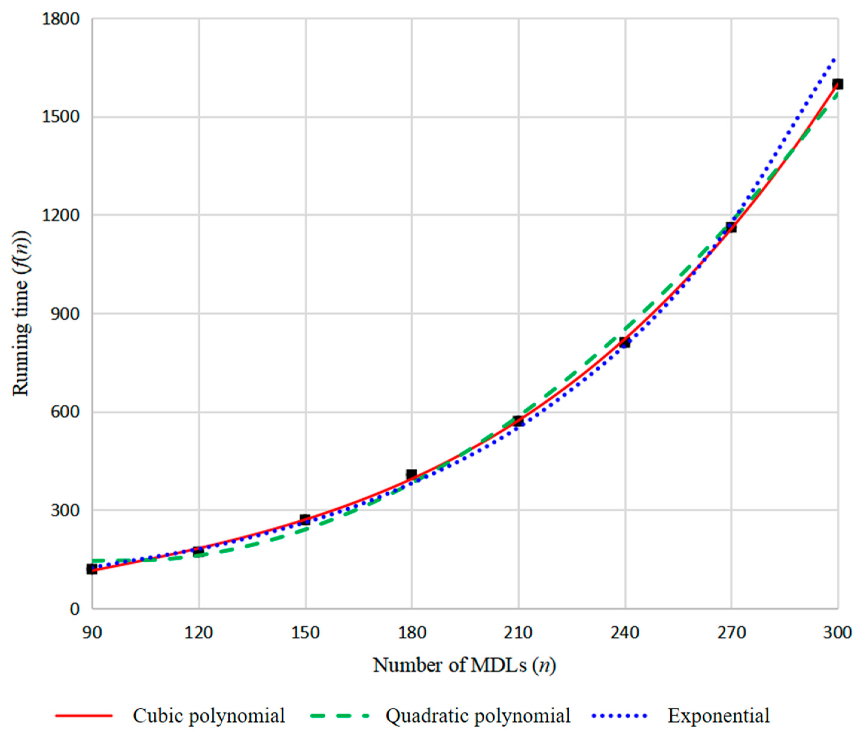
| MDL Scale | Total Travel Time (h) | Running Time (s) |
|---|---|---|
| 90 | 53.81 | 119.91 |
| 120 | 74.73 | 172.58 |
| 150 | 98.9 | 270.15 |
| 180 | 118.7 | 407.84 |
| 210 | 134.61 | 570.98 |
| 240 | 160.28 | 811.16 |
| 270 | 179.09 | 1162.41 |
| 300 | 202.74 | 1598.78 |
| Parameter | Value |
|---|---|
| Rated power of PV | 180 kW |
| Rated power of diesel generator | 200 kW |
| Maximum value of battery SOC | 400 kWh |
| Minimum value of battery SOC | 120 kWh |
| Loss cost of PV power generation | 0.3 CNY/kWh |
| Cost of diesel | 6.4 CNY/L |
| Loss cost of battery charging and discharging | 0.3 CNY/kWh |
| Carbon tax rate | 0.14 CNY/kg |
| Carbon emission factor | 3.315 |
| Diesel intercept coefficient | 0.01609 |
| Diesel slope coefficient | 0.2486 |
| Battery charging efficiency | 85% |
| Battery discharge efficiency | 100% |
| Condition | Period | |||||||||||||
|---|---|---|---|---|---|---|---|---|---|---|---|---|---|---|
| 1 | 2 | 3 | 4 | 5 | 6 | 7 | 8 | 9 | 10 | 11 | 12 | 13 | 14 | |
| Sailing 1 | 0 | 0 | 0 | 0 | 0 | 0 | 0 | 0 | 0.1 | 1 | 0.5 | 0 | 0 | 0 |
| Sailing 2 | 0 | 0 | 0 | 0.42 | 1 | 1 | 0 | 0 | 0 | 0 | 0 | 0 | 0 | 0 |
| Sailing 3 | 1 | 0.13 | 0.55 | 0 | 0 | 0 | 0 | 0.7 | 0 | 0 | 0 | 0.22 | 0.08 | 0.56 |
| Working | 0 | 0.87 | 0.45 | 0.58 | 0 | 0 | 1 | 0.3 | 0.9 | 0 | 0.5 | 0.78 | 0.92 | 0 |
| Vessel No. | Period | |||||||||||||
|---|---|---|---|---|---|---|---|---|---|---|---|---|---|---|
| 1 | 2 | 3 | 4 | 5 | 6 | 7 | 8 | 9 | 10 | 11 | 12 | 13 | 14 | |
| 1 | 160 | 73.26 | 114.94 | 48.35 | 32.12 | 32.12 | 60 | 130.15 | 57.08 | 30.41 | 45.21 | 81.58 | 68.42 | 90.31 |
| 2 | 160 | 91.53 | 130.63 | 60 | 28.89 | 20.03 | 67.95 | 97.34 | 60 | 69.35 | 68.55 | 82.41 | 77.59 | 115.66 |
| 3 | 82.67 | 118.9 | 71.6 | 60 | 43.18 | 30.41 | 80 | 99.75 | 61.82 | 77.78 | 68.89 | 84.15 | 85.85 | 17.36 |
| 4 | 80 | 86.09 | 83.78 | 78.41 | 0 | 0 | 0 | 0 | 0 | 0 | 0 | 0 | 0 | 0 |
| 5 | 103.29 | 75.13 | 78.26 | 73.33 | 56.23 | 0 | 0 | 0 | 0 | 0 | 0 | 0 | 0 | 0 |
| 6 | 92.8 | 73.22 | 84.35 | 60 | 119.63 | 15.73 | 0 | 0 | 0 | 0 | 0 | 0 | 0 | 0 |
| Scenario | Period | |||||||||||||
|---|---|---|---|---|---|---|---|---|---|---|---|---|---|---|
| 1 | 2 | 3 | 4 | 5 | 6 | 7 | 8 | 9 | 10 | 11 | 12 | 13 | 14 | |
| A | 80 | 90 | 100 | 140 | 160 | 180 | 150 | 120 | 90 | 80 | 60 | 35 | 20 | 0 |
| B | 70 | 80 | 90 | 120 | 140 | 160 | 130 | 100 | 80 | 70 | 50 | 30 | 15 | 0 |
| C | 40 | 50 | 60 | 90 | 110 | 130 | 100 | 70 | 50 | 40 | 30 | 15 | 5 | 0 |
| Scenario | Vessel No. | Total | |||||
|---|---|---|---|---|---|---|---|
| 1 | 2 | 3 | 4 | 5 | 6 | ||
| A | 572.17 | 680.93 | 445.89 | 98.49 | 163.17 | 166.28 | 2126.93 |
| B | 634.59 | 739.67 | 514.24 | 137.43 | 181.83 | 180.35 | 2388.1 |
| C | 918.93 | 1127.79 | 820.8 | 344.94 | 343.62 | 331.5 | 3887.58 |
| Item (kW) | Period | |||||||||||||
|---|---|---|---|---|---|---|---|---|---|---|---|---|---|---|
| 1 | 2 | 3 | 4 | 5 | 6 | 7 | 8 | 9 | 10 | 11 | 12 | 13 | 14 | |
| Load demand | 160 | 73.26 | 114.94 | 48.35 | 32.12 | 32.12 | 60 | 130.15 | 57.08 | 30.41 | 45.21 | 81.58 | 68.42 | 90.31 |
| PV-Load | 59.16 | 73.26 | 90 | 48.35 | 32.12 | 32.12 | 60 | 100 | 57.08 | 30.41 | 45.21 | 30 | 15 | 0 |
| PV-Battery | 10.84 | 6.74 | 0 | 71.65 | 100 | 100 | 5.35 | 0 | 0 | 0 | 0 | 0 | 0 | 0 |
| Diesel-Load | 100.84 | 0 | 0 | 0 | 0 | 0 | 0 | 0 | 0 | 0 | 0 | 0 | 0 | 0 |
| Battery-Load | 0 | 0 | 24.94 | 0 | 0 | 0 | 0 | 30.15 | 0 | 0 | 0 | 51.58 | 53.42 | 90.31 |
| SOC | 139.21 | 144.94 | 120 | 180.91 | 265.91 | 350.91 | 355.46 | 325.31 | 325.31 | 325.31 | 325.31 | 273.73 | 220.31 | 130 |
| Case | Time Windows |
|---|---|
| 1.1 | [7, 10] |
| 1.2 | [13, 15] |
| 1.3 | [17.5, 19.5] |
| 2.1 | [13, 15], [17.5, 19.5] |
| 2.2 | [7, 10], [17.5, 19.5] |
| 2.3 | [7, 10], [13, 15] |
| 3 (baseline) | [7, 10], [13, 15], [17.5, 19.5] |
Disclaimer/Publisher’s Note: The statements, opinions and data contained in all publications are solely those of the individual author(s) and contributor(s) and not of MDPI and/or the editor(s). MDPI and/or the editor(s) disclaim responsibility for any injury to people or property resulting from any ideas, methods, instructions or products referred to in the content. |
© 2025 by the authors. Licensee MDPI, Basel, Switzerland. This article is an open access article distributed under the terms and conditions of the Creative Commons Attribution (CC BY) license (https://creativecommons.org/licenses/by/4.0/).
Share and Cite
Chen, L.; Duan, G.; Cao, J.; Wang, J. Two-Stage Optimization on Vessel Routing and Hybrid Energy Output for Marine Debris Collection. Sustainability 2025, 17, 3425. https://doi.org/10.3390/su17083425
Chen L, Duan G, Cao J, Wang J. Two-Stage Optimization on Vessel Routing and Hybrid Energy Output for Marine Debris Collection. Sustainability. 2025; 17(8):3425. https://doi.org/10.3390/su17083425
Chicago/Turabian StyleChen, Li, Gang Duan, Jie Cao, and Jinhua Wang. 2025. "Two-Stage Optimization on Vessel Routing and Hybrid Energy Output for Marine Debris Collection" Sustainability 17, no. 8: 3425. https://doi.org/10.3390/su17083425
APA StyleChen, L., Duan, G., Cao, J., & Wang, J. (2025). Two-Stage Optimization on Vessel Routing and Hybrid Energy Output for Marine Debris Collection. Sustainability, 17(8), 3425. https://doi.org/10.3390/su17083425