A Whole-Stand Model for Estimating the Productivity of Uneven-Aged Temperate Pine-Oak Forests in Mexico

Abstract

This study presents a model for estimating forest productivity based on a sample of 2048 permanent field plots covering a wide range of growing sites in Mexico. Our state-space approach assumes that the growth behavior of any stand over time can be estimated on the basis of its current state, defined by the dominant height (H), number of trees per hectare (N), and stand basal area (BA). We used transition functions to estimate the change in states as a function of the current state. We also present transition functions for the change in stand volume (V) and total above-ground biomass (AGB). The first transition function relates dominant height to dominant diameter by using the guide-curve method to estimate site form. The transition function for N consists of two models, one for estimating natural mortality and the other for estimating recruitment. These models were developed in two steps: in the first step, the logistic regression and maximum likelihood approach were used to estimate the probability of the occurrence of mortality or recruitment, and in the second step, the rate of change associated with each event was modeled when mortality or recruitment was assumed to have occurred as a result of the first step. The remaining three transition functions (BA, V, and AGB) were fitted simultaneously to account for possible correlations between errors. The model estimating total above-ground biomass (AGB), which can be considered a state variable that summarizes the performance of the whole model, explained more than 97% of the observed variability, with a root mean square error value of 10.57 Mg/ha.

1. Introduction

Forest ecosystems store large amounts of biomass, provide habitats for countless wild species [1,2], and provide a variety of goods and services [3,4] that are essential for sustaining environmental, economic, and social stability in many regions of the world [5,6,7]. Forest ecosystems are often managed, and decision-making aimed at reconciling biodiversity conservation, wood production, and mitigation strategies requires quantifiable information about how they change over time [8,9].

The forests of Mexico include diverse types of woody plants that occur in a variety of climates within a wide range of altitudes and latitudes [10,11]. Two biogeographic regions merge in the country: the Nearctic region in the north and the Neotropical region in the south [12]. This combination has created a high level of biological diversity in Mexico, which is considered a megadiverse region and unique biodiversity hotspot [13,14,15] and is one of 12 countries that include between 60% and 70% of the total biodiversity in the world [16]. Special attention should be given to temperate forests, which provide habitats for thousands of plant and animal species, owing to the tropical influence and the wide altitudinal range. Temperate forests in Mexico are considered the most biodiverse in the world [11,17]. Temperate forests cover 22% of the country’s total land area [18], and they are found in five “Sierras” known as the “Sierra Madre Occidental” (SMO), the “Sierra Madre Oriental” (SMOr), the “Sistema Neovolcánico Transversal” (SNT), the “Sierra Madre Sur” (SMS), and the “Sierra Madre Centroamericana y altos de Chiapas” (SMCACh). The dominant tree species in these forests belong to the genera Pinus and Quercus.

According to Davies et al. [7], climate change mitigation largely depends on the permanence of forest land and on carbon capture in forests. The forest ecosystems in Mexico are susceptible to climate change and continuing anthropogenic disturbance [19,20]. Intensive forest biomass production can lead to loss, degradation, and reshuffling of biodiversity [21,22,23]. Changes in forest ecosystems over time are affected by tree growth and mortality as well as the recruitment of new trees. Understanding these processes is essential to sustaining the goods and services provided by forest ecosystems. Therefore, forest monitoring and the development and continuous improvement of growth models that estimate changes in the forests are essential for the conservation and sustainable management of these key resources [9].

Whole-stand growth models are among the tools most frequently used to estimate tree growth and forest production [24,25]. The models used for even-aged forest plantations have gradually been improved over time [26,27,28]. However, not all forests are pure and even-aged, and growth and yield models are required for different types of forests and for multiple purposes at different spatial scales (national, stand, and landscape). This is especially true for the structurally heterogeneous temperate forests of Mexico, characterized by a wide range of ages, species, and mixtures of tree sizes. The inability to use age as a reference variable represents a major challenge in estimating the dynamics of mixed and uneven-aged forests. In addition, the estimation of recruitment is important, as it is considered negligible in most models developed for pure and even-aged forest plantations.

The information provided by forest observational infrastructures, which require a long-term commitment to ensure a steady flow of field observations supported by appropriate assessment and archiving protocols [29], is used as the quantitative basis for developing forest growth and yield models. The objective of the present study was, therefore, to propose a methodology for developing robust and biologically meaningful whole-stand growth and yield models for the mixed and uneven-aged temperate forests in Mexico. The data used were obtained from an extensive network of permanent plots which form part of the unique observational infrastructure of the forests under study.

2. Materials and Methods

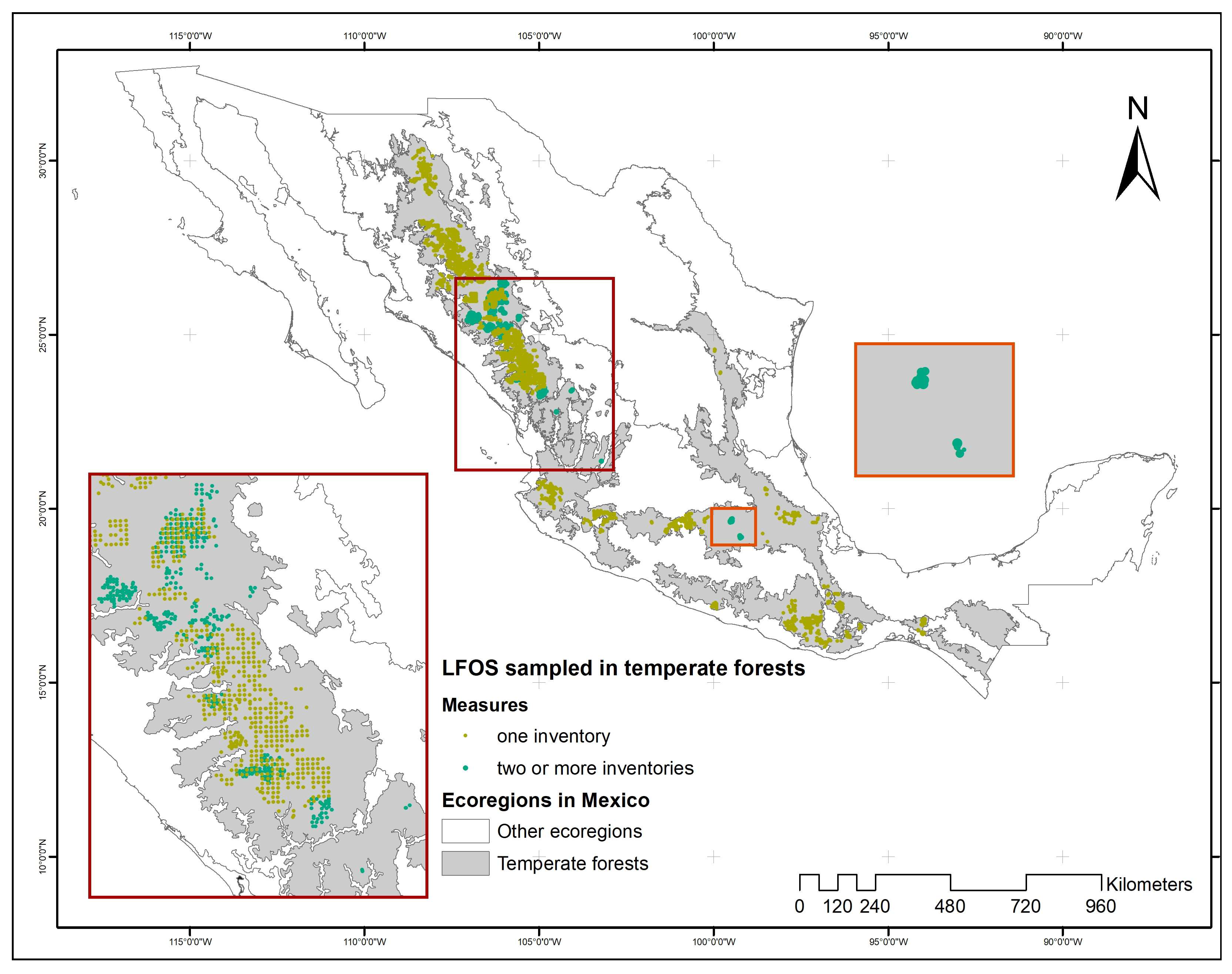
2.1. Data

The data used in this study were provided by a long-term forest observational infrastructure (LFOI) that currently includes a total of 2048 forest plots in Mexico. The distribution of the plots is semi-systematic, with square grids between 3 and 5 km and plots located at the margin of the grid, in order to obtain information on tree formations with a spatial distribution that is difficult to cover with systematic sampling. Most of the plots are located within the temperate forest ecoregion (TeF).

The observational network covers a latitudinal range between 16.021 and 30.333 decimal degrees and a longitudinal range between −108.681 and −93.938 decimal degrees (see Figure 1). The altitudinal range includes plots located between 466 and 3514 masl, with a mean of 2252 masl. The mean annual temperature in the study area varies between 9.42 and 27.32 °C, with an average of 16.4 °C. The mean annual precipitation varies between 914 and 1420 mm/year, with an average of 1003.1 mm/year [30].

All plots are square, and the size varies according to the number of trees per hectare, in order to yield a sufficient number of samples to produce robust estimates of stand variables. The LFOI includes 1865 plots of 0.25 ha and 183 plots of 0.625 ha. The establishment of the sample plots began in 2009 and continued until 2018, while remeasurements began in 2012 and continued until 2021. To facilitate data management, a computer platform was developed in 2016 (http://fcfposgrado.ujed.mx/monafor/inicio/, accessed on 27 February 2025), to allow the field data to be uploaded directly from a mobile app and to allow users (generally forest managers) to ask different questions and conduct numerical and graphical analyses.

The protocol developed by Corral-Rivas et al. [31] was used for both plot establishment and sample measurement. In each sample plot, trees of breast height diameter (dbh) greater than or equal to 7.5 cm were measured. Two perpendicular measurements of dbh were made with the aid of a caliper, and tree heights were measured with a hypsometer. Tree species were identified by a botanist, who also recorded the stage of development of the trees. Each tree was tagged at the height of the dbh measurement to facilitate remeasurement.

A total of 292 tree species were identified, and the genera Pinus (28 species) and Quercus (67 species) were found to be the most common. Among the pines, Pinus duranguensis Ehren, Pinus arizonica Engelm, Pinus teocote Schiede ex Schltdl., Pinus cooperi C.E. Blanco, and Pinus leiophylla Schl. & Cham. were the most abundant species. Of the oaks, Quercus sideroxyla Bonpl., Quercus crassifolia Bonpl., Quercus rugosa Née, Quercus arizonica Sarg., and Quercus fulva Liebm. were the most common species. Together, these two genera represent 86% of all the trees measured. Other genera such as Arbutus and Juniperus were also relatively abundant and frequent (4.9 and 4.6% of the total number of trees measured, respectively).

A number of stand variables were calculated from the tree diameter and height data: the number of trees per ha (N); basal area (BA, m²/ha); quadratic mean diameter (dg, cm); dominant height (H, m) and dominant diameter (D, cm), calculated as the mean height and mean dbh of the 100 thickest trees per hectare, respectively; the relative spacing index (RSI), calculated as the ratio between the mean distance between trees and the dominant height $RSI=100/\left(H·\sqrt{N}\right)$; stand density index $SDI=N·{\left(dg/25\right)}^{1.605}$, trees/ha); stand volume (V, m³/ha), calculated from the volumes of each tree estimated with the equations proposed for each species in the study area by Vargas-Larreta et al. [32]; and above-ground biomass (AGB, Mg/ha), calculated from the biomass of each tree estimated with the species-specific equations for the study area [33].

Of the 2048 sample plots, those in which Pinus or Quercus was the dominant genus (in terms of percentage basal area) were selected, yielding a total of 1984 plots (1564 plots were dominated by Pinus and 420 plots by Quercus). In order to take into account the possible effect of the mixture of genera on stand development, the percentage basal area of the genus Pinus in each sample plot (%BA_Pinus) was also included as a potential predictor variable.

To date, only a portion of the total of 1984 sample plots of mixed pine-oak forest have been remeasured. In addition, some of the remeasured plots were excluded from the study as they showed evidence of different types of disturbance, i.e., natural (pests, diseases, fires) and/or anthropogenic (harvesting operations). The data used in the study therefore include single measurements made in 1527 sample plots, two successive measurements made in 352 sample plots, and three successive measurements made in 105 sample plots, for a total of 2546 field inventories and 562 non-overlapping growth intervals (see Figure 1). The time between successive measurements varied between 4 and 7.03 years, with a mean value of 5.30 years. The mean, maximum, minimum, and standard deviation of the main stand variables for the total field inventories and for each of the remeasurements are shown in

Table 1. Descriptive statistics of the main stand variables of the sample plots used to develop the dynamic growth model of the mixed temperate pine-oak forests. The mean ± standard deviation (minimum–maximum) are shown for each variable.

Variable	All Data (2444 Field Inventories)	Sample Plots with Remeasurements
		First Remeasurement (457 Field Inventories)	Second Remeasurement (105 Field Inventories)
N (trees/ha)	474.19 ± 253.99 (20–2264)	646.89 ± 291.08 (120–2264)	651.04 ± 294.44 (144–2152)
BA (m2/ha)	18.67 ± 10.48 (0.37–75.09)	20.59 ± 7.21 (3.1–43.34)	23.14 ± 8.09 (3.92–51.65)
dg (cm)	23.14 ± 6.87 (8.42–54.42)	20.78 ± 4.03 (12.37–34.43)	21.97 ± 4.12 (13.02–37.88)
H (m)	15.9 ± 6.63 (3.36–41.3)	16.25 ± 4.05 (5.26–24.89)	17.85 ± 4.4 (5.83–28)
D (cm)	34.71 ± 9.6 (8.66–74.7)	35.1 ± 6.28 (17.99–54.89)	36.88 ± 6.39 (20–57.09)
RSI	0.36 ± 0.25 (0.08–3.29)	0.28 ± 0.16 (0.12–1.63)	0.28 ± 0.17 (0.12–1.39)
SDI (trees/ha)	423.70 ± 196.27 (9.10–1560.52)	459.40 ± 162.67 (73.57–976.68)	477.71 ± 177.93 (90.66–1047.89)
V (m3/ha)	172.36 ± 141.6 (2.04–927.93)	180.16 ± 89.63 (11.68–485.91)	218.41 ± 107.59 (16–594.9)
AGB (Mg/ha)	109.99 ± 77.87 (1.82–510.26)	113.31 ± 46.45 (11.76–256.35)	130.61 ± 52.69 (15.7–304.72)
%BAPinus	63.32 ± 23.63 (0–100)	67.56 ± 15.78 (32.24–100)	67.42 ± 15.26 (30.19–100)

N: stand density (trees/ha); BA: stand basal area (m²/ha); dg: quadratic mean diameter (cm); H: dominant height (m); D: dominant diameter (cm); RSI: relative spacing index; SDI: stand density index (trees/ha); V: stand volume (m³/ha); AGB: stand above-ground biomass (Mg/ha); %BA_Pinus: percentage basal area of Pinus genera.

.

2.2. Modeling Approach

The method used to develop the whole-stand production model is based on the state-space approach described by García [34], which uses state variables to characterize the system at an initial stage and transition functions to project all or some of the state variables to future states. As the stands are generally uneven-aged, age cannot be used as an input variable in the development of the model.

A three-dimensional vector including dominant height (H), stand density (N), and stand basal area (BA) as state variables was found to be sufficient to describe the stand condition at a given time using three transition functions. Thus, the outputs of these three transition functions would provide the inputs of static functions to predict the stand volume or stand above-ground biomass at a given point in time. Nevertheless, given the wide range of forest structures and species mixtures, we decided to also develop transition functions for stand volume (V) and above-ground biomass (AGB).

2.2.1. Transition Function for Dominant Height (H)

As it is not possible to use age, site quality was estimated from the relationship between height and diameter at the stand level [35,36]; in this case, the values of dominant diameter (D) and dominant height (H) were used, and the site quality indicator is referred to as site form [8,37]. The dominant height transition function or site quality model must satisfy a series of requirements including polymorphism, a sigmoid growth pattern with an inflection point, the existence of a horizontal asymptote at old ages or logical behavior (the height must be 1.3 m at dominant diameter zero and equal to site form at the reference dominant diameter).

As most of the sample plots have a single inventory with a single pair of data (D,H), the site quality model was developed in two steps by using the guide-curve method [38], for which the complete field measurement database was used. In the first step, a base equation was fitted to the D and H pairs, thus yielding the average H−D relationship. In the second step, the family of site form curves were generated by making each of the base equation parameters dependent on the local site form (local parameter), defined as the value of H at a given reference value of D. Thus, each base equation generates as many site form family curves as parameters in the base equation formulation. Three well-known base equations used in the development of site quality models were used in the fitting process, namely, the Bertalanffy equation [39,40], the Hossfeld equation [41], and the Korf equation [42], and all possible resultant families of site form family curves were generated.

The formulation of the base equation and the mathematical expression of the transition function derived from each, depending on the local parameter selected, are shown in

Table 2. Base equations used to develop the site quality curves and mathematical expression of the transition functions derived from each base equation depending on the local parameter selected. H₁ and D₁ are dominant height and dominant diameter at time t₁ and H₂ and D₂ are the same variables at time t₂.

Base Equation	Local Parameter	Transition Function
Bertalanffy [39,40] $H=1.3+a{·\left(1-e^{-b·D}\right)}^c$	$a={\displaystyle \frac{H_1-1.3}{{\left(1-e^{-b·D_1}\right)}^c}}$	${\widehat{H}}_2=1.3+{\displaystyle \frac{H_1-1.3}{{\left(1-e^{-b·D_1}\right)}^c}}·{\left(1-e^{-b·D_2}\right)}^c$
	$b={\displaystyle \frac{-log\left[1-{\left(\left(H_1-1.3\right)/a\right)}^{\raisebox{1ex}{$1$}\!\left/ \!\raisebox{-1ex}{$c$}\right.}\right]}{D_1}}$	${\widehat{H}}_2={1.3+a·\left[1-exp\left(log\left(1-{\left({\displaystyle \frac{H_1-1.3}{a}}\right)}^{{\displaystyle \raisebox{1ex}{$1$}\!\left/ \!\raisebox{-1ex}{$c$}\right.}}\right){\displaystyle \frac{D_2}{D_1}}\right)\right]}^c$
	$c={\displaystyle \frac{log\left(\left(H_1-1.3\right)/a\right)}{log\left(1-e^{-b·D_1}\right)}}$	${\widehat{H}}_2=1.3+a{·\left(1-e^{-b·D_2}\right)}^{{\displaystyle \frac{log\left(\left(H_1-1.3\right)/a\right)}{log\left(1-e^{-b·D_1}\right)}}}$
Hossfeld [41] $H=1.3+{\displaystyle \frac{D^2}{{\left(a+b·D\right)}^2}}$	$a={\displaystyle \frac{D_1}{\sqrt{H_1-1.3}}}-b·D_1$	${\widehat{H}}_2=1.3+{\displaystyle \frac{D_1^2}{{\left(\frac{D_1}{\sqrt{H_1-1.3}}+b·\left(D_2-D_1\right)\right)}^2}}$
	$b={\displaystyle \frac{D_1/\sqrt{H_1-1.3}-a}{D_1}}$	${\widehat{H}}_2=1.3+{\displaystyle \frac{D_1^2}{{\left(a+\frac{D_1/\sqrt{H_1-1.3}-a}{D_1}·D_2\right)}^2}}$
Korf [42] $H={1.3+e}^{a-b/D^c}$	$a=log\left(H_1-1.3\right)+{\displaystyle \raisebox{1ex}{$b$}\!\left/ \!\raisebox{-1ex}{$D_1^c$}\right.}$	${\widehat{H}}_2={1.3+e}^{log\left(H_1-1.3\right)-b·\left({\displaystyle \raisebox{1ex}{$1$}\!\left/ \!\raisebox{-1ex}{$D_2^c$}\right.}-{\displaystyle \raisebox{1ex}{$1$}\!\left/ \!\raisebox{-1ex}{$D_1^c$}\right.}\right)}$
	$b=\left(a-log\left(H_1-1.3\right)\right)·D_1^c$	${\widehat{H}}_2={1.3+e}^{a-\left(a-log\left(H_1-1.3\right)\right)·{\displaystyle \frac{D_1^c}{D_2^c}}}$
	$c={\displaystyle \frac{log\left(b/\left(a-log\left(H_1-1.3\right)\right)\right)}{log\left(D_1\right)}}$	${\widehat{H}}_2={1.3+e}^{a-b/D_2^{{\displaystyle \frac{log\left(b/\left(a-log\left(H_1-1.3\right)\right)\right)}{log\left(D_1\right)}}}}$

. The selection of the best combination between the base equation and the local parameter for obtaining the transition function was based on visual inspection of the performance of the curves superimposed on the observed data and the values of two goodness-of-fit statistics: model efficiency (ME) and root mean square error (RMSE).

$$ME={\rho }_{y_i\widehat{y_i}}^2$$

$$RMSE=\sqrt{{\displaystyle \frac{\sum _{i=1}^n{\left(y_i-\widehat{y_i}\right)}^2}{n-1}}}$$

where y_i is the observed value of the dependent variable in each remeasurement, $\widehat{y_i}$ is the value estimated for that remeasurement using the transition function, ${\rho }_{y_i\widehat{y_i}}$ is the linear correlation coefficient between both values, and n is the number of remeasurements.

2.2.2. Transition Function for the Number of Trees per Unit Area (N)

In a state of natural stand development, without considering natural or anthropogenic disturbance, the variation in the number of trees per hectare between two points in time will depend on two simultaneous processes: natural mortality (defined as the probability of mortality just for competence causes) and recruitment (defined here as the probability of survival of new individuals that have reached 7.5 cm in diameter at the second point in time). In a given sample plot, either one, both or neither of these processes may occur, and each will have the opposite effect on the change in the number of trees per hectare. In this study, tree mortality was observed in 91.45% of the growth intervals of the 457 sample plots with more than one measurement, and recruitment was observed in 85.69% of the sample plots.

As they have opposite effects on the future number of trees per hectare, natural mortality and recruitment were modeled separately and then combined to optimize the results of their estimates. A two-step approach was used in both cases. In the first step, an equation was fitted to predict the probability of survival of all trees in the stand (in the case of natural mortality) and another equation was fitted to estimate the probability of no new trees being incorporated to the stand (in the case of recruitment), considering all of the sample plots with more than one measurement. In the second step, a transition function was developed to estimate the reduction in stand density due to natural mortality (using data from the sample plots where this occurred) and another transition function was used to determine the increase in stand density due to recruitment (using data from the sample plots where this occurred).

Both natural mortality and recruitment are discrete events in which only values of 0 (non-event) or 1 (event) are possible. Therefore, a function that provides probability estimates to model both processes was applied. Although several cumulative distribution functions would be appropriate, the logistic function is the most commonly used in models of this type. The logistic model is formulated as follows:

$$\pi ={\left[{\displaystyle \frac{e^{\left({\alpha }_0+{\alpha }_1·x_1+\cdots +{\alpha }_i·x_i\right)}}{1+e^{\left({\alpha }_0+{\alpha }_1·x_1+\cdots +{\alpha }_i·x_i\right)}}}\right]}^{∆t}$$

where α_i are the parameters and x_i are the independent variables. When the above equation is fitted to natural mortality data (event (1) is the absence of natural mortality and non-event (0) is the presence of natural mortality), π represents the probability of survival of all trees in a plot (i.e., mortality is given by 1 − π) in a time interval of Δt years. In the case of fitting the logistic equation to recruitment data (event is non-incorporation of new trees and non-event is incorporation of new trees) π represents the probability of no recruitment in a plot (i.e., recruitment is given by 1 − π) in a time interval of Δt years.

As the remeasurement intervals of the sample plots were irregular, a weighted logistic function including the exponent Δt was used to account for time [43]. Thus, in this equation, as the time interval increases, the probability of mortality also gradually increases when fitted to natural mortality data. When fitted to recruitment data, the probability of new trees being incorporated gradually increases.

The estimates of the parameters for each process were obtained by maximizing the logarithm of the likelihood function of the logistic model, as follows:

$$l\left(\widehat{\pi },{\alpha }_i\right)=-\sum _{j=1}^{n_1}∆t·log\left({\displaystyle \frac{e^{\left({\alpha }_0+{\alpha }_1·x_{1j}+\cdots +{\alpha }_i·x_{ij}\right)}}{1+e^{\left({\alpha }_0+{\alpha }_1·x_{1j}+\cdots +{\alpha }_i·x_{ij}\right)}}}\right)-\sum _{j=1}^{n_0}log\left(1-{\left({\displaystyle \frac{e^{\left({\alpha }_0+{\alpha }_1·x_{1j}+\cdots +{\alpha }_i·x_{ij}\right)}}{1+e^{\left({\alpha }_0+{\alpha }_1·x_{1j}+\cdots +{\alpha }_i·x_{ij}\right)}}}\right)}^{∆t}\right)$$

where α_i are the parameters and x_i are the independent variables, n₁ is the number of remeasurements with an observed event over a period of Δt years, and n₀ is the number of remeasurements without observed events in the same period.

The selection of the best set of independent variables for each of the two processes was based on the knowledge of the factors influencing these processes combined with the application of the stepwise method of variable selection.

Once the probability of the occurrence of either process has been determined, the second step of the modeling consists of fitting a transition function to estimate the change in the number of trees per hectare between two time instants for each process separately (in the case of natural mortality, this will imply a reduction in N and in the case of recruitment, it will imply an increase in N). In this study, we tested eight models based on two basic differential equations:

$${\displaystyle \frac{1}{N}}·{\displaystyle \frac{∆N}{∆H}}=\alpha ·N^{\beta }·f\left(SF,\%{BA}_{Pinus}\right)·H^{\delta }$$

$${\displaystyle \frac{1}{N}}·{\displaystyle \frac{∆N}{∆H}}=\alpha ·\left[f\left(SF,\%{BA}_{Pinus}\right)+{\displaystyle \frac{\delta }{H}}\right]$$

where α, β, and δ are parameters that regulate the rates of change and f(SF, %BA_Pinus) is a linear function of site form and percentage of basal area of the genus Pinus: $f\left(SF,\%{BA}_{Pinus}\right)=c_0+c_1·SF+c_2·\%{BA}_{Pinus}.$

The first differential equation implies that the relative rate of change in the number of trees is proportional to the power function of H. The integration of this equation with the initial condition δ ≠ 1 gives the following two algebraic difference models depending on the value of β:

$$\beta \ne 0\hspace{1em}{N}_2={\left[N_1^{b_1}+f\left(SF,\%{BA}_{Pinus}\right)·\left(H_2^{b_2}-H_1^{b_2}\right)\right]}^{{\displaystyle \frac{1}{b_1}}}$$

with b₁ = −β and b₂ = δ + 1:

$$\beta =0\hspace{1em}{N}_2=N_1·e^{f\left(SF,\%{BA}_{Pinus}\right)·\left(H_2^{b_1}-H_1^{b_1}\right)}$$

with b₁ = δ + 1.

The six different transition functions derived from the first differential equation and proposed by Clutter and Jones [44], Pienaar and Shiver [45], Pienaar et al. [46], Tomé et al. [47], Woollons [48], and García [49] were applied (see Table 3).

The second differential equation implies that the relative rate of change in the number of trees is proportional to a hyperbolic function of H. The integration of that equation gives the following algebraic difference form:

$$N_2=N_1·{\left({\displaystyle \frac{H_2}{H_1}}\right)}^{b_1}·e^{f\left(SF,\%{BA}_{Pinus}\right)·\left(H_2-H_1\right)}$$

with b₁ = δ·α.

Two transition functions based on this solution and proposed by Bailey et al. [50] and Zunino and Ferrando [51] were assessed (Table 3).

Table 3. Transition functions used to model the variation in the number of trees per hectare between two points in time due to natural mortality and to recruitment.

Author	Initial Condition	Mathematical Expression of the Transition Function
Clutter and Jones (1980) [44]	β ≠ 0	${\widehat{N}}_2={\left[N_1^{b_1}+f\left(SF,\%{BA}_{Pinus}\right)·\left[{\left(\frac{{\widehat{H}}_2}{100}\right)}^{b_2}-{\left(\frac{H_1}{100}\right)}^{b_2}\right]\right]}^{{\displaystyle \raisebox{1ex}{$1$}\!\left/ \!\raisebox{-1ex}{$b_1$}\right.}}$
Pienaar et al. (1990) [46]	β ≠ 0	${\widehat{N}}_2={\left[N_1^{b_1}+f\left(SF,\%{BA}_{Pinus}\right)·\left[{\left(\frac{{\widehat{H}}_2}{10}\right)}^{b_2}-{\left(\frac{H_1}{10}\right)}^{b_2}\right]\right]}^{{\displaystyle \raisebox{1ex}{$1$}\!\left/ \!\raisebox{-1ex}{$b_1$}\right.}}$
Woollons (1998) [48]	β = 0.5	${\widehat{N}}_2={\left[N_1^{-0.5}+f\left(SF,\%{BA}_{Pinus}\right)·\left[{\left(\frac{{\widehat{H}}_2}{100}\right)}^2-{\left(\frac{H_1}{100}\right)}^2\right]\right]}^{-2}$
García (2013) [49]	β ≠ 0	${\widehat{N}}_2={\left[N_1^{b_1}+\frac{f\left(SF,\%{BA}_{Pinus}\right)}{b_2}·\left({\widehat{H}}_2^{b_2}-H_1^{b_2}\right)\right]}^{{\displaystyle \raisebox{1ex}{$1$}\!\left/ \!\raisebox{-1ex}{$b_1$}\right.}}$
Pienaar and Shiver (1981) [45]	β = 0	${\widehat{N}}_2=N_1·e^{f\left(SF,\%{BA}_{Pinus}\right)·\left[{\left(\frac{{\widehat{H}}_2}{100}\right)}^{b_1}-{\left(\frac{H_1}{100}\right)}^{b_1}\right]}$
Tomé et al. (1997) [47]	β = 0	${\widehat{N}}_2=N_1·e^{f\left(SF,\%{BA}_{Pinus}\right)·\left({\widehat{H}}_2-H_1\right)}$
Zunino and Ferrando (1997) [51]	β = 0	${\widehat{N}}_2=N_1·{\left(\frac{{\widehat{H}}_2}{H_1}\right)}^{b_1}·e^{f\left(SF,\%{BA}_{Pinus}\right)·\left({\widehat{H}}_2-H_1\right)}$
Bailey et al. (1985) [50]	β = 0	${\widehat{N}}_2=N_1·{\left(\frac{{\widehat{H}}_2}{H_1}\right)}^{b_1}·e^{\left(f\left(SF,\%{BA}_{Pinus}\right)·\left({\widehat{H}}_2-H_1\right)\right)}$

Table 3. Transition functions used to model the variation in the number of trees per hectare between two points in time due to natural mortality and to recruitment.

Author	Initial Condition	Mathematical Expression of the Transition Function
Clutter and Jones (1980) [44]	β ≠ 0	${\widehat{N}}_2={\left[N_1^{b_1}+f\left(SF,\%{BA}_{Pinus}\right)·\left[{\left(\frac{{\widehat{H}}_2}{100}\right)}^{b_2}-{\left(\frac{H_1}{100}\right)}^{b_2}\right]\right]}^{{\displaystyle \raisebox{1ex}{$1$}\!\left/ \!\raisebox{-1ex}{$b_1$}\right.}}$
Pienaar et al. (1990) [46]	β ≠ 0	${\widehat{N}}_2={\left[N_1^{b_1}+f\left(SF,\%{BA}_{Pinus}\right)·\left[{\left(\frac{{\widehat{H}}_2}{10}\right)}^{b_2}-{\left(\frac{H_1}{10}\right)}^{b_2}\right]\right]}^{{\displaystyle \raisebox{1ex}{$1$}\!\left/ \!\raisebox{-1ex}{$b_1$}\right.}}$
Woollons (1998) [48]	β = 0.5	${\widehat{N}}_2={\left[N_1^{-0.5}+f\left(SF,\%{BA}_{Pinus}\right)·\left[{\left(\frac{{\widehat{H}}_2}{100}\right)}^2-{\left(\frac{H_1}{100}\right)}^2\right]\right]}^{-2}$
García (2013) [49]	β ≠ 0	${\widehat{N}}_2={\left[N_1^{b_1}+\frac{f\left(SF,\%{BA}_{Pinus}\right)}{b_2}·\left({\widehat{H}}_2^{b_2}-H_1^{b_2}\right)\right]}^{{\displaystyle \raisebox{1ex}{$1$}\!\left/ \!\raisebox{-1ex}{$b_1$}\right.}}$
Pienaar and Shiver (1981) [45]	β = 0	${\widehat{N}}_2=N_1·e^{f\left(SF,\%{BA}_{Pinus}\right)·\left[{\left(\frac{{\widehat{H}}_2}{100}\right)}^{b_1}-{\left(\frac{H_1}{100}\right)}^{b_1}\right]}$
Tomé et al. (1997) [47]	β = 0	${\widehat{N}}_2=N_1·e^{f\left(SF,\%{BA}_{Pinus}\right)·\left({\widehat{H}}_2-H_1\right)}$
Zunino and Ferrando (1997) [51]	β = 0	${\widehat{N}}_2=N_1·{\left(\frac{{\widehat{H}}_2}{H_1}\right)}^{b_1}·e^{f\left(SF,\%{BA}_{Pinus}\right)·\left({\widehat{H}}_2-H_1\right)}$
Bailey et al. (1985) [50]	β = 0	${\widehat{N}}_2=N_1·{\left(\frac{{\widehat{H}}_2}{H_1}\right)}^{b_1}·e^{\left(f\left(SF,\%{BA}_{Pinus}\right)·\left({\widehat{H}}_2-H_1\right)\right)}$

These equations were fitted using the value estimated with the transition function of the dominant height (${\widehat{H}}_2$) as the value of the dominant height at time t₂ instead of the value measured in the field in the remeasurements (H₂), in order to adapt the fitting of the different transition functions to the sequence followed when the whole-stand growth model is applied to a new stand. The selection of the best transition function for each of the processes (natural mortality and recruitment) was based on the graphical analysis of the residuals and the ME and RMSE values.

The application of the logistic equations (first step) to a new plot enables the estimation of two probabilities: one for natural mortality and one for recruitment. These probabilities are compared with specific thresholds for each process and, if they are lower than the threshold, the event does not occur, i.e., there is no mortality or no recruitment and the stand density does not change; otherwise, the event occurs, and the transition function of the process is used to determine the change in stand density (second step).

Finally, the future stand density will be obtained by combining the results of natural mortality and recruitment and the thresholds of each process were optimized so that the sum of squares of the errors (difference between the observed and estimated stand density values in the remeasurements) is minimal.

2.2.3. Transition Function for Basal Area (BA)

The basal area transition function was derived from a differential equation assuming that the rate of change in the basal area for a given dominant height depends on the initial basal area (BA) and the dominant height (H):

$${\displaystyle \frac{dBA}{dH}}=a_1·H^{a_2}·{BA}^{a_3}$$

The same model was used by Álvarez-González et al. [52]. A similar expression, but including the stand age, was used by Borders and Bailey [53], Pienaar et al. [46], and Forss [54].

Integrating both sides of the differential equation gives the following invariant:

$${BA}^{1-a_3}-{\displaystyle \frac{a_1·\left(1-a_3\right)}{a_2+1}}·H^{a_2+1}=C$$

This invariant can be used to generate the transition function by equating the corresponding invariants and solving for BA₂:

$${BA}_2={\left[{BA}_1^{1-a_3}+{\displaystyle \frac{a_1·\left(1-a_3\right)}{a_2+1}}·\left(H_2^{a_2+1}-H_1^{a_2+1}\right)\right]}^{1/(1-a_3)}$$

2.2.4. Transition Function for Stand Volume and Above-Ground Biomass

Both stand volume (V) and stand above-ground biomass (AGB) can be fitted to the same biologically-based differential equation structure that represents a generic production variable W. The variation in this variable between two points in time, relative to the dominant height dW/dH will depend on two components: net growth and loss of growth due to natural mortality. According to Álvarez-González et al. [52], a simple closed form can be used to estimate the rate of change in this generic variable considering both components, as follows:

$${\displaystyle \frac{dW}{dH}}=b_1·H^{b_2}·{BA}^{b_3}+b_3·{\displaystyle \frac{W}{BA}}·{\displaystyle \frac{dBA}{dH}}$$

Substituting BA and dBA/dH in the previous equation for the expressions obtained in Section 2.2.3 and grouping the terms and integrating both sides gives the following invariant:

$${W·BA}^{-b_3}-b_1·{\displaystyle \frac{H^{b_2+1}}{b_2+1}}=C$$

Finally, the following algebraic difference equation was obtained by considering the status of the stand at two different times and solving for W₂:

$${\widehat{W}}_2=\left[{W_1·BA}_1^{-b_3}+{\displaystyle \frac{b_1}{b_2+1}}·\left({\widehat{H}}_2^{b_2+1}-H_1^{b_2+1}\right)\right]·{\widehat{BA}}_2^{b_3}$$

This expression was used as a transition function for both stand volume (W = V) and above-ground biomass (W = AGB).

Dominant height and basal area are independent variables in their transition functions but dependent variables in other transition functions. The resulting cross dependence between these functions can cause errors due to violation of the assumption independence, and the set of transition functions should thus be fitted simultaneously. However, as the structure of the database used to fit the site quality curves differs from the others, the first transition function was fitted separately and the estimated remeasurements of the sample plots $\widehat{H_2}$ were used in the remaining transition functions instead of the observed values (H₂).

Furthermore, due to the special structure of the transition function for N, which takes into account two processes (natural mortality and recruitment), and because both were modeled in two steps, this transition function was also fitted separately. Finally, the other three transition functions (BA, V, and AGB) were fitted simultaneously to eliminate the bias of simultaneous equations using the full information maximum likelihood (FIML). Parameter estimation was carried out with the MODEL procedure of SAS/ETS^® [55].

3. Results and Discussion

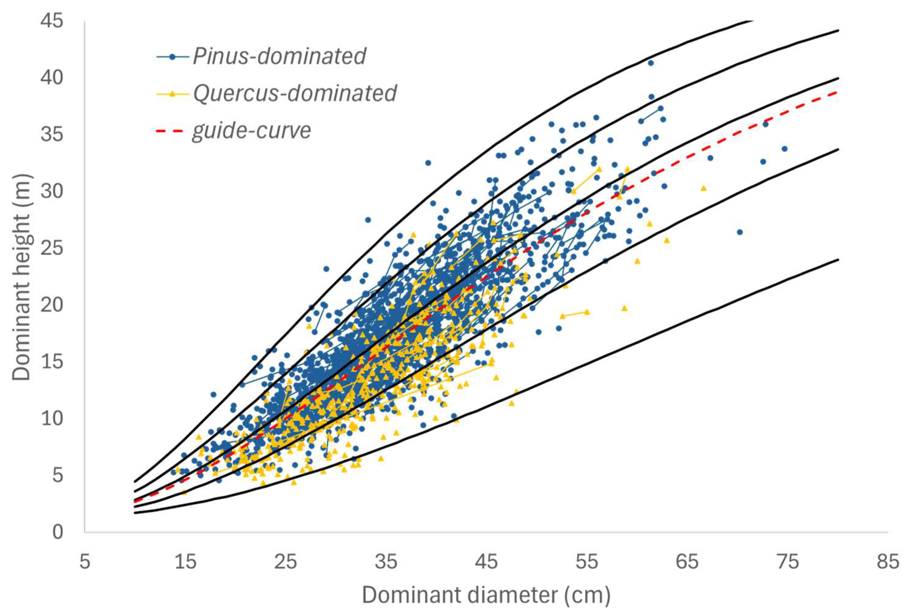
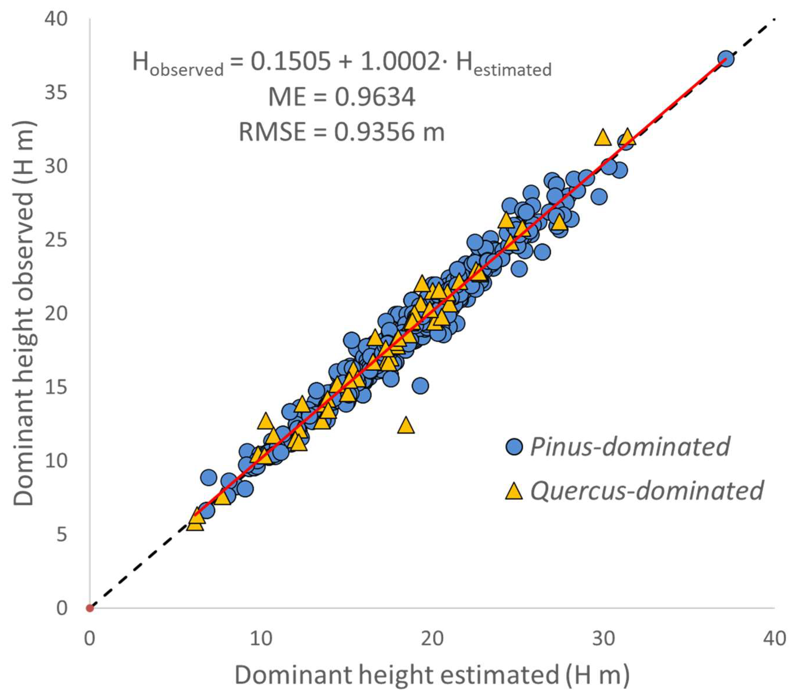
3.1. Transition Function for Dominant Height (H)

The results of the guide-curve fitting method conducted using the base models of Bertalanffy [39,40], Hossfeld [41], and Korf [42] are very similar, with ME values varying between 0.7474 for the Hossfeld base model and 0.7493 for the Bertalanffy base model and RMSE values ranging from 3.0564 to 3.0453 m for the same base models, respectively (

Table 4. Parameter estimates and goodness-of-fit statistics of the three base models used to fit the guide curve.

Model	a	b	c	ME	RMSE (m)	RMSE (%)
Bertalanffy	50.9920	0.0268	2.4630	0.7493	3.0453	18.49
Hossfeld	6.4397	0.0747	---	0.7474	3.0564	18.56
Korf	5.3065	−19.1039	0.5615	0.7484	3.0509	18.53

). In all three cases, all parameters were significant (α = 0.05).

The values of the goodness-of-fit statistics are similar to those obtained in other studies using the guide-curve methodology to develop site quality curves. For example, Ahmedi et al. [56] developed site form curves for uneven-aged and mixed forest dominated by oriental beech (Fagus orientalis Lipsky) in Hyrcanian Forests (Iran) using the Bertalanffy model, obtaining ME and RMSE values of 0.755 and 3.30 m, respectively. Molina-Valero et al. [57] developed site form curves for mature silver fir, beech and mixed species forests in Spain by using the Hossfeld and Bertalanffy base models, obtaining ME values varying between 0.29 for beech forests and 0.66 for silver fir forests with RMSE values between 4.08 and 2.58 m for the same species, respectively. Aguirre et al. [58] used the guide-curve method and the Bertalanffy and Hossfeld models to fit site form curves for 24 forest types dominated by different species in Spain, obtaining statistical goodness-of-fit values of the same order as those obtained in the present study.

The final selection of one of the three base models will therefore depend on the performance of the family of curves when overlaid on the data of the measurements used to fit the guide curve. The best results were obtained with the Bertalanffy base model, in which the value of parameter b is considered the local parameter, with parameters a and c being global. The resulting family of curves is polymorphic, with a common horizontal asymptote. This asymptote has a very high value (more than 50 m in height) and therefore the curves are not affected by this common condition, within the range of dominant diameter values reached in this type of mixed forest (see Figure 2). According to Bailey and Clutter [59], the effective limit will depend on the lifespan of the species under study and therefore will not be constant across values of SF. Families of curves with similar characteristics have been widely used in studies of site index curves, e.g., [60,61].

Figure 2 shows the original data with isolated points corresponding to sample plots with a single measurement and lines corresponding to the trends observed in sample plots with more than one measurement. A distinction is also made between plots dominated by the genus Pinus and those dominated by the genus Quercus, in terms of basal area. The guide curve (dashed red line) and five examples of curves corresponding to site form values of 6, 10, 14, 18, and 22 m for a dominant reference diameter of 30 cm (solid black lines) were superimposed on the data.

As shown in the figure, the lowest site quality observed (dominant height of 6 m for a dominant diameter of 30 cm) mainly corresponds to sample plots in which the genus Quercus dominates, while the highest quality (22 m for a diameter of 30 cm) was mainly observed in sample plots in which the genus Pinus dominates. This may be attributable, on the one hand, to the higher quality requirements of most of the predominant pine species in these pine-oak forests and, on the other hand, to the difference in the height-diameter ratio between species of these two genera. These differences initially led us to fit different models by the dominant genus. However, considering that the observed trends in the sample plots with several measurements are similar for both dominant genera and the good performance of the fitted curves for intermediate site qualities (the most frequently observed), this led us to accept the validity of a single family of curves for the whole dataset.

A similar approach has also been used by other authors in the development of site form curves in uneven-aged mixed forests with a large diversity of species, e.g., [38,62,63], assuming that estimation of the SF while considering all species may capture the variability in growth of dominant height (H) among tree species and thus site conditions [37]. Nonetheless, this approach will only describe whole-stand productivity and cannot be used to estimate the growth potential of a specific species. In the future, when more sample plots and, in particular, greater numbers of remeasurements become available (enhancing our understanding of the observed trends), the models must be redesigned using more precise methodologies such as the algebraic differences approach (ADA) or the generalized algebraic differences approach (GADA). The need to develop different models for dominant genera or even for groups of dominant species within each genus will also need to be further evaluated.

The final expression of the transition function for the dominant height is as follows:

$${\widehat{H}}_2={1.3+50.9920·\left[1-exp\left(log\left(1-{\left({\displaystyle \frac{H_1-1.3}{50.9920}}\right)}^{{\displaystyle \raisebox{1ex}{$1$}\!\left/ \!\raisebox{-1ex}{$2.4630$}\right.}}\right){\displaystyle \frac{D_2}{D_1}}\right)\right]}^{2.4630}$$

(1)

where H₁ and D₁ are the dominant height (m) and dominant diameter (cm) at the beginning of the growth period and H₂ and D₂ are the same values at the end of the growth period. The general equation for estimating the site form for any given pine-oak forest is as follows:

$$\widehat{SF}={1.3+50.9920·\left[1-exp\left(log\left(1-{\left({\displaystyle \frac{H_1-1.3}{50.9920}}\right)}^{{\displaystyle \raisebox{1ex}{$1$}\!\left/ \!\raisebox{-1ex}{$2.4630$}\right.}}\right){\displaystyle \frac{30}{D_1}}\right)\right]}^{2.4630}$$

(2)

To evaluate the performance of the aforementioned transition function, the values of the dominant height in the remeasurements were estimated from the previous inventory data, and the observed values were compared with the estimated values (see Figure 3). The model explains more than 96% of the observed variability, with an RMSE value of 0.94 m. Although the model performs very well, these values are somewhat lower than those usually obtained when permanent plot or stem analysis data are available and the algebraic difference (ADA) or generalized algebraic difference (GADA) approximations are used. It can be seen in the figure that the trends for Pinus-dominated and Quercus-dominated plots are similar, supporting the decision to fit a single family of curves for all of the sampled plots. In addition, there was no evident over- or underestimation of values.

The values of $\widehat{H_2}$ estimated with Equation (1) were used instead of the field measurements to develop the remaining transition functions; the same applies to the values of site form estimated with Equation (2).

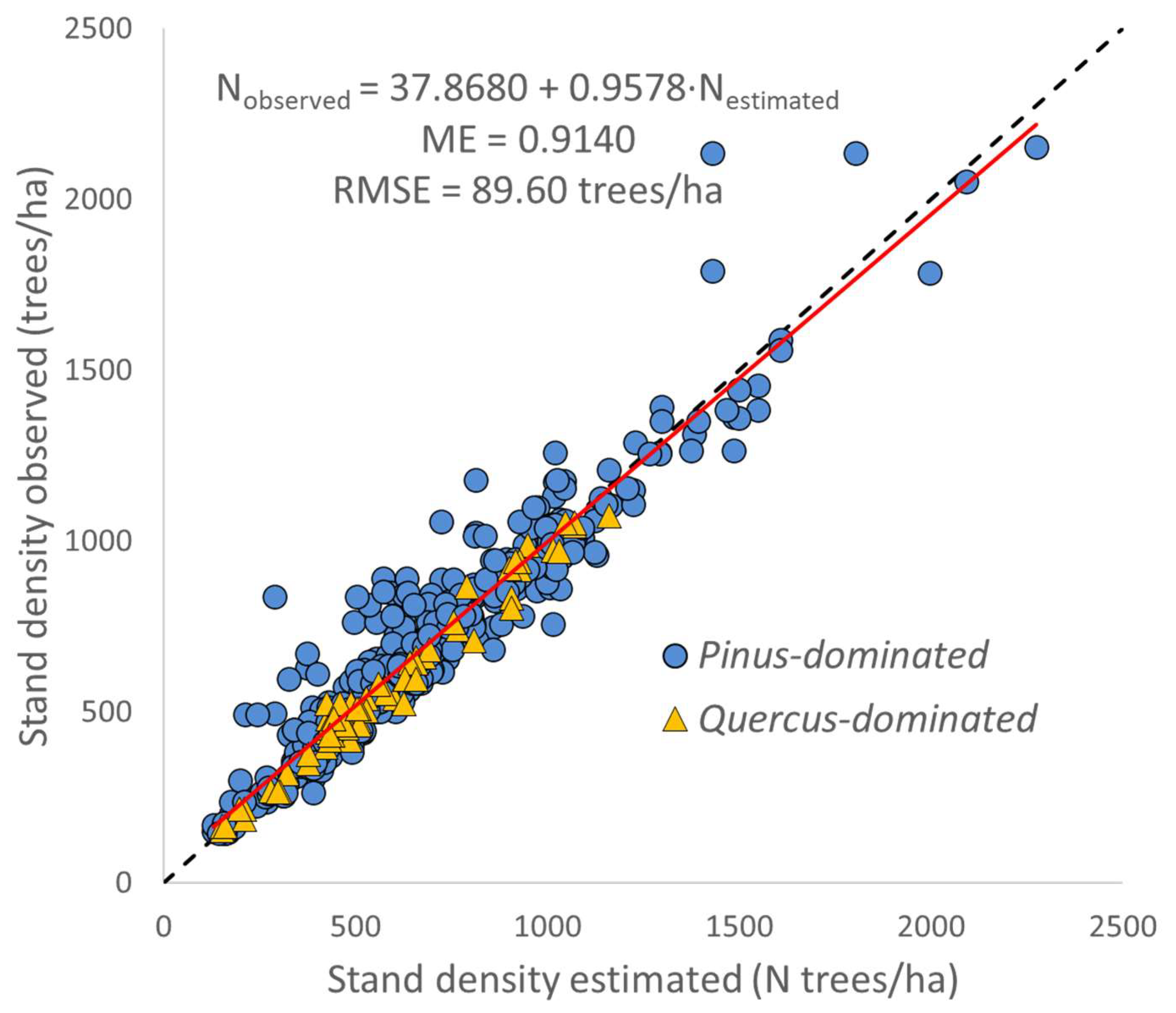
3.2. Transition Function for Stand Density (N)

The change in the number of trees per hectare over a period of time (Δt) in this type of uneven-aged mixed forest depends on two different processes: natural mortality and recruitment. Each of these processes was modeled separately as they do not both occur at the same time in all sample plots and, therefore, each sample is different.

However, both natural mortality and recruitment are discrete events in which only values of 0 (absence) or 1 (presence) can be given. In the first case, the stand density does not vary, while it does vary in the second case and must be estimated. Thus, each process was first modeled by using an equation that estimates the probability of the occurrence of the event and, if this probability exceeds a fixed deterministic threshold (presence of the event), another equation is used to estimate the change in stand density.

3.2.1. Models for Estimating Natural Mortality

As the probability of the occurrence of natural mortality increases over time, the fitted logistic model estimates the probability $\left(\widehat{\pi }\right)$ of no natural mortality occurrence in the time interval (Δt), and therefore the probability that it does occur will equal 1 − $\widehat{\pi }$. The results of using the stepwise method of variable selection, together with the knowledge of the factors affecting the natural mortality process, suggest the inclusion of the initial stand density (N), the site form value (SF), and the relative spacing index (RSI). These variables have frequently been used to estimate the probability of the occurrence of natural mortality, e.g., [48,64,65,66].

The parameter estimators were obtained by minimizing the value of the maximum likelihood function and the equation finally obtained is as follows:

$${\widehat{\pi }}_{mort}=1-{\left[{\displaystyle \frac{e^{\left(-1.5884-0.0001079·N+0.1248·SF+1.6339·RSI\right)}}{1+e^{\left(-1.5884-0.0001079·N+0.1248·SF+1.6339·RSI\right)}}}\right]}^{∆t}$$

(3)

All parameters were significant (α = 5%) and their signs consistent with the biological behavior of this type of forest, so that, all other things being equal, when stand density (N) increases, the probability of natural mortality increases. When site form (SF) increases, the probability of natural mortality decreases, and when competition decreases and, therefore, the value of the relative spacing index (RSI) increases, the probability of natural mortality decreases. The percentage of concordant pairs of the model was 70.01%.

Once the logistic model was fitted, the data from the sample plots in which natural mortality was observed were used to fit the transition function of the reduction in the number of trees per hectare ${\widehat{N}}_{2\_mort}=f\left(N_1,H_1,{\widehat{H}}_2,\widehat{SF},\%{BA}_{Pinus}\right)$ using the models listed in Table 3. The parameter associated with the basal area of the genus Pinus was not significant in any of the models analyzed. The best results were obtained with the model proposed by Bailey et al. [50], and the final expression of the transition function for the reduction in the number of trees per hectare due to natural mortality is as follows:

$${\widehat{N}}_{2\_mort}=N_1·{\left({\displaystyle \frac{{\widehat{H}}_2}{H_1}}\right)}^{-0.7378}·e^{0.0002554·SF·\left({\widehat{H}}_2-H_1\right)}$$

(4)

All parameters were significant, and the model explained 98.62% of the observed variability, with an RMSE value of 32.98 trees/ha. The values of these goodness-of-fit statistics are comparable to those obtained in similar studies that used age instead of dominant height as a time step variable. For example, Maleki et al. [67] reported values of ME between 0.96 and 0.98 for broadleaf forests and forests dominated by Norway spruce, respectively, with RMSE ranging from 69.48 to 143.26 trees/ha for pine and broadleaf forests, respectively for growth models of three forest types dominated by Picea sitchensis, Pinus sylvestris, and a mixture of Betula spp. with other broadleaf species in Norway, using a model with the same structure as Equation (4).

3.2.2. Models for Estimating Recruitment

In the case of recruitment, the probability of the occurrence of the event increases as the time between measurements (Δt) increases. Thus, the probability ($\widehat{\pi }$) that recruitment will not occur can be estimated by the logistic equation, and the probability that it will occur will be given by 1 − $\widehat{\pi }$. The results of the stepwise method of variable selection, together with information about the factors affecting recruitment, suggested the inclusion of the initial quadratic mean diameter (dg) and the relative spacing index (RSI) as explanatory variables. The quadratic mean diameter and stand variables related to competition have frequently been used as explanatory variables in models estimating recruitment probability. For example, Lexerød [68] used initial stand density (N) and stand basal area (BA), among other variables, as explanatory variables in logistic models developed to estimate the probability of recruitment in different forest types in Norway. Fortin and De Blois [69] used stand basal area in a probability model including the Weibull density function at Hardwood Stands in Southern Québec, Canada. Zhang et al. [70] used negative binomial mixture models including the initial mean stand diameter and basal area (among other variables) as explanatory variables to predict the recruitment of Chinese pine (Pinus tabulaeformis) in Beijing (China). Finally, Maleki et al. [67] included the initial quadratic mean diameter and stand density as explanatory variables in a recruitment probability estimation equation used in growth models developed for different forest types in Norway.

The parameter estimates were obtained by minimizing the value of the maximum likelihood function, and the equation finally obtained is as follows:

$${\widehat{\pi }}_{rec}=1-{\left[{\displaystyle \frac{e^{\left(-0.8718+0.06661·d_g+0.8818·RSI\right)}}{1+e^{\left(-0.8718+0.06661·d_g+0.8818·RSI\right)}}}\right]}^{∆t}$$

(5)

All parameters were significant (α = 5%) and their signs consistent with the biological behavior of this type of forest. The percentage of concordant pairs for this model was 62.95%.

Once the logistic model was fitted, the data from the sample plots in which recruitment was observed were used to fit the transition function of increment in the number of trees per hectare ${\widehat{N}}_{2\_rec}=f\left(N_1,H_1,{\widehat{H}}_2,\widehat{SF},\%{BA}_{Pinus}\right)$ using the models shown in Table 3. As in the case of the transition function, and owing to natural mortality, the parameter associated with the basal area of the genus Pinus was not significant in any of the models analyzed. The best results were also obtained in this case with the model proposed by Bailey et al. [50], and the final expression of the transition function for the increment in the number of trees per hectare due to recruitment is as follows:

$${\widehat{N}}_{2\_rec}=N_1·{\left({\displaystyle \frac{{\widehat{H}}_2}{H_1}}\right)}^{0.6802}·e^{0.0002536·SF·\left({\widehat{H}}_2-H_1\right)}$$

(6)

All parameters were significant, and the model explained 95.18% of the observed variability, with an RMSE value of 66.25 trees/ha.

Once the four Equations (3)–(6) were obtained, the procedure based on a deterministic approach was used to estimate the stand density after a time interval (Δt). First, the estimated probability of natural mortality ${(\widehat{\pi }}_{mort})$ was compared with a fixed threshold (p_mort), where ${\widehat{\pi }}_{mort}>p_{mort}$ indicates that the event has occurred and the estimated stand density reduction is given by Equation (4), where ${\widehat{\pi }}_{mort}\le p_{mort}$ indicates that the initial stand density has not changed due to natural mortality, i.e., ${\widehat{N}}_{2\_mort}=N_1$. Similarly, the estimated probability of recruitment $\left({\widehat{\pi }}_{rec}\right)$ was compared with a different fixed threshold (p_rec) and, when ${\widehat{\pi }}_{rec}>p_{rec}$, the increase in stand density was estimated by Equation (6) and, otherwise, the initial stand density was assumed not to have changed due to recruitment, i.e., ${\widehat{N}}_{2\_rec}=N_1$. Finally, the density at the end of the time interval is given by the expression:

$${\widehat{N}}_2={{\widehat{N}}_{2\_mort}+{\widehat{N}}_{2\_rec}-N}_1$$

(7)

The optimal values of both thresholds were estimated as those that minimize the sum of squares of the differences between the observed values of stand density in the remeasurements (N₂) and those obtained with Equation (7) for all possible combinations of thresholds with values between 0.01 and 0.99 with 0.01 intervals. The optimal values of these thresholds are p_mort = 0.85 and p_rec = 0.64. The overall accuracy of Equation (3) in estimating whether or not natural mortality occurs with a threshold of 0.85 is 84.72%, and the overall accuracy of Equation (5) in estimating whether or not recruitment occurs with a threshold of 0.64 is 85.61%.

Figure 4 shows the distribution of observed stand density versus estimated values obtained with Equation (7) distinguished between Pinus-dominated and Quercus-dominated sample plots. The model explains more than 91% of the observed variability, with an RMSE value of 89.60 trees/ha. The figure shows similar trends for Pinus-dominated and Quercus-dominated sample plots, indicating that %BA_Pinus did not have an explanatory capacity in the models of stand density change as a consequence of natural mortality or recruitment (Equations (4) and (6)). Furthermore, as in the case of the dominant height transition function, no pattern of over- or underestimation was observed.

3.3. Transition Functions for Stand Basal Area (BA), Stand Volume (V), and Above-Ground Biomass (AGB)

Three transition functions were initially fitted separately to obtain a parameter estimate that was then used as an input value in the simultaneous fitting of the three-equation system using the full information maximum likelihood (FIML) approach. The following transition functions were obtained in the simultaneous fitting:

$${\widehat{BA}}_2={\left[{BA}_1^{1.0734}+25.2049·\left({\widehat{H}}_2^{1.1935}-H_1^{1.1935}\right)\right]}^{1/1.0734}$$

(8)

$${\widehat{V}}_2=\left[{V_1·BA}_1^{0.00848}+112.5665·\left({\widehat{H}}_2^{1.5934}-H_1^{1.5934}\right)\right]·{\widehat{BA}}_2^{-0.00848}$$

(9)

$${\widehat{AGB}}_2=\left[{{AGB}_1·BA}_1^{0.00265}+77.2466·\left({\widehat{H}}_2^{1.4824}-H_1^{1.4824}\right)\right]·{\widehat{BA}}_2^{-0.00265}$$

(10)

All parameters were significant (α = 5%), and the transition functions explained 96.07%, 96.88%, and 97.05% of the observed variability in stand basal area (BA), stand volume (V), and stand above-ground biomass (AGB), respectively (see Figure 5). RMSE values of 1.79 m²/ha, 22.22 m³/ha, and 10.57 Mg/ha were obtained for the same variables.

Again, these results do not show any obvious differences in the data trends according to the dominant genus or any tendency for over- or underestimation of the three dependent variables.

The values of the goodness-of-fit statistics are within the range observed in other models with a similar structure. For example, García et al. [71] developed a model for loblolly pine plantations in the USA using a more complex structure than in the present study, and including site occupancy, obtaining an RMSE value in the estimate of BA of 1.73 m²/ha. In addition, Garcia [49] developed a model for regular thinned and unthinned trembling aspen stands in Western Canada, using the same complex structure but replacing the age with the dominant diameter, as in the present study, and obtaining an RMSE value of 3.03 m²/ha in BA estimates. Álvarez-González et al. [52] obtained ME values of 0.6721 and 0.8512 for BA and AGB with a model developed for pure and even-aged stands of Pinus pinaster in North-Western Spain using the same transition functions as those used in the present study; however, it should be noted that the time intervals between measurements were longer than the intervals used in the present study, resulting in greater uncertainty and lower precision. Tewari et al. [72] obtained an ME of 0.9956 in estimates of stand basal area for teak plantations in India with limited data (22 sample plots) with a whole-stand growth model structure similar to the model proposed here, but using age instead of dominant diameter. Finally, Maleki et al. [67] fitted a whole-stand growth model (also including recruitment) for the three main forest types in Norway (spruce, pine, and broadleaf species), obtaining ME values between 0.978 and 0.991 for BA and between 0.977 and 0.986 for V.

4. Conclusions

In this study, a whole-stand model was developed for temperate, mixed, and uneven-aged oak-pine forests. The state-space approach was used, considering three main state variables: the dominant height, the number of trees per hectare, and the basal area. The model consists of 10 equations that enable estimation of the change in the three state variables as well as in two other fundamental variables related to production: stand volume and above-ground biomass. The fact that the variation in the number of trees over time was modeled by combining two natural processes, natural mortality and recruitment, is of particular importance. Overall, the system of equations yields accurate estimates of all the state variables and only requires a number of input variables that are simple to measure in a single field inventory. In addition, these same input variables could be obtained by remote sensing, which would enable the use of the model to map the current state and evolution of these forests at landscape scale.

Although the database used is very extensive and covers a large variety of environmental and management conditions, the high variability in the structure and specific composition of the forests under study require the continual establishment of new plots and, in particular, remeasurement of existing sample plots. This will enable the model to be improved by using the same structure of relationships developed in this study.

Observations covering longer time intervals would enable, among other things, a more robust assessment of the effect of Pinus or Quercus dominance. This effect was not evident in the proposed model, probably due to the insufficient time intervals between measurements. Increasing the number of remeasurements will also enable the use of more accurate modeling approaches for site quality curves such as the algebraic difference approach (ADA) or the generalized algebraic differences approach (GADA). The estimation of the future dominant height is used as an input value in all the other transition functions developed, and the accurate estimation of this variable is therefore essential.

Moreover, the addition of new information will enable the assessment of the need to develop more detailed models, such as individual tree models that can be applied at smaller spatial scales and that are specific to genus or even to species or communities of species.

Finally, climate and other environmental changes will alter future rates of forest growth, mortality and recruitment; therefore, long-term forest management decisions must be based on growth and yield models that incorporate climate effects. Thus, the models presented here should be adapted in the future by including not only field information from new plots and remeasurements, but also climatic variables and/or other environmental factors (e.g., atmospheric CO₂ concentration or N deposition) to account for this effect in model estimates.

References

1. Zhang, T.; Niinemets, U.; Sheffield, J.; Lichstein, J.W. Shifts in Tree Functional Composition Amplify the Response of Forest Biomass to Climate. Nature 2018, 556, 99–102. [Google Scholar] [CrossRef] [PubMed]
2. Blundo, C.; Carilla, J.; Grau, R.; Malizia, A.; Malizia, L.; Osinaga-Acosta, O.; Bird, M.; Bradford, M.; Catchpole, D.; Ford, A.; et al. Taking the Pulse of Earth’s Tropical Forests Using Networks of Highly Distributed Plots. Biol. Conserv. 2021, 260, 108849. [Google Scholar] [CrossRef]
3. Geijzendorffer, I.R.; Cohen-Shacham, E.; Cord, A.F.; Cramer, W.; Guerra, C.; Martín-López, B. Ecosystem Services in Global Sustainability Policies. Environ. Sci. Policy 2017, 74, 40–48. [Google Scholar] [CrossRef]
4. Feurer, M.; Rueff, H.; Celio, E.; Heinimann, A.; Blaser, J.; Htun, A.M.; Zaehringer, J.G. Regional scale mapping of ecosystem services supply, demand, flow and mismatches in southern Myanmar. Ecosyst. Serv. 2021, 52, 101363. [Google Scholar] [CrossRef]
5. Díaz, S.; Pascual, U.; Stenseke, M.; Martín-López, B.; Watson, R.T.; Molnár, Z.; Hill, R.; Chan, K.M.; Baste, I.A.; Brauman, K.A.; et al. Assessing nature’s contributions to people. Science 2018, 359, 270–272. [Google Scholar] [CrossRef]
6. Aguirre-Gutiérrez, J.; Rifai, S.; Shenkin, A.; Oliveras, I.; Bentley, L.P.; Svátek, M.; Girardin, C.A.; Both, S.; Riutta, T.; Berenguer, E.; et al. Pantropical Modelling of Canopy Functional Traits Using Sentinel-2 Remote Sensing Data. Remote Sens. Environ. 2021, 252, 112122. [Google Scholar] [CrossRef]
7. Davies, S.J.; Abiem, I.; Salim, K.A.; Aguilar, S.; Allen, D.; Alonso, A.; Anderson-Teixeira, K.; Andrade, A.; Arellano, G.; Ashton, P.S.; et al. ForestGEO: Understanding Forest Diversity and Dynamics through a Global Observatory Network. Biol. Conserv. 2021, 253, 108907. [Google Scholar] [CrossRef]
8. Vanclay, J. Modelling Forest Growth and Yield: Applications to Mixed Tropical Forests; CAB International: Wallingford, UK, 1994; 330p. [Google Scholar]
9. Randin, C.F.; Ashcroft, M.B.; Bolliger, J.; Cavender-Bares, J.; Coops, N.C.; Dullinger, S.; Dirnböck, T.; Eckert, S.; Ellis, E.; Fernández, N.; et al. Monitoring Biodiversity in the Anthropocene Using Remote Sensing in Species Distribution Models. Remote Sens. Environ. 2020, 239, 111626. [Google Scholar] [CrossRef]
10. Rzedowski, J. Vegetación de México, 1st ed.; Limusa: Mexico City, Mexico, 1978. [Google Scholar]
11. Rzedowski, J. Diversidad y orígenes de la flora fanerogámica de México. Acta Bot. Mex. 1991, 14, 3–21. [Google Scholar] [CrossRef]
12. Rzedowski, J.; Reyna-Trujillo, T. Provincias Florísticas; Instituto de Geografía, Universidad Nacional Autónoma de México: Mexico City, Mexico, 1990. [Google Scholar]
13. Sarukhán, J.; Dirzo, R. México Ante los Retos de la Biodiversidad; Comisión Nacional para el Conocimiento y Uso de la Biodiversidad: Tlalpan, Mexico, 1992.
14. Feeley, K.J.; Davies, S.J.; Pérez, R.; Hubbell, S.P.; Foster, R.B. Directional changes in the species composition of a tropical forest. Ecology 2011, 92, 871–882. [Google Scholar] [CrossRef]
15. Harfoot, M.B.; Johnston, A.; Balmford, A.; Burgess, N.D.; Butchart, S.H.; Dias, M.P.; Hazin, C.; Hilton-Taylor, C.; Hoffmann, M.; Isaac, N.J.B.; et al. Using the IUCN Red List to map threats to terrestrial vertebrates at global scale. Nat. Ecol. Evol. 2021, 5, 1510–1519. [Google Scholar] [CrossRef] [PubMed]
16. Brooks, T.M.; Mittermeier, R.A.; Da Fonseca, G.A.B.; Gerlach, J.; Hoffmann, M.; Lamoreux, J.F.; Mittermeier, C.G.; Pilgrim, J.D.; Rodrigues, A.S.L. Global biodiversity conservation priorities. Science 2006, 313, 58–61. [Google Scholar] [CrossRef] [PubMed]
17. González-Elizondo, M.S.; González Elizondo, M.; Márquez Linares, M. Vegetación y Ecorregiones de Durango; Centro Interdisciplinario de Investigación para el Desarrollo Integral Regional (CIIDIR), Instituto Politécnico Nacional: Durango, Mexico, 2007. [Google Scholar]
18. INEGI-CONABIO. Ecorregiones Terrestres de México. 2008. Available online: https://geoportal.conabio.gob.mx/metadatos/doc/html/ecort08gw.html (accessed on 27 February 2025).
19. Lebrija-Trejos, E.; Pérez-García, E.A.; Meave, J.A.; Poorter, L.; Bongers, F. Environmental changes during secondary succession in a tropical dry forest in Mexico. J. Trop. Ecol. 2011, 27, 477–489. [Google Scholar] [CrossRef]
20. Ellis, T.; Bowman, D.; Williamson, G. Humans have substantially extended fire seasons in all biomes on Earth. Res. Sq. 2025. [Google Scholar] [CrossRef]
21. Powers, R.P.; Jetz, W. Global habitat loss and extinction risk of terrestrial vertebrates under future land-use-change scenarios. Nat. Clim. Change 2019, 9, 323–329. [Google Scholar] [CrossRef]
22. Daskalova, G.N.; Myers-Smith, I.H.; Bjorkman, A.D.; Blowes, S.A.; Supp, S.R.; Magurran, A.E.; Dornelas, M. Landscape-scale forest loss as a catalyst of population and biodiversity change. Science 2020, 368, 1341–1347. [Google Scholar] [CrossRef] [PubMed]
23. Chase, J.M.; Blowes, S.A.; Knight, T.M.; Gerstner, K.; May, F. Ecosystem decay exacerbates biodiversity loss with habitat loss. Nature 2020, 584, 238–243. [Google Scholar] [CrossRef]
24. Burkhart, H.E.; Tomé, M. Modeling Forest Trees and Stands; Springer: Dordrecht, The Netherlands, 2012. [Google Scholar]
25. Gadow, K.v.; Álvarez-González, J.G.; Zhang, C.; Pukkala, T.; Zhao, X. Sustaining Forest Ecosystems; Springer Nature: Cham, Switzerland, 2021. [Google Scholar]
26. Weiskittel, A.R.; Hann, D.W.; Kershaw, J.A.; Vanclay, J.K. Forest Growth and Yield Modeling; John Wiley & Sons: Oxford, UK, 2011. [Google Scholar]
27. da Rocha, S.J.; Torres, C.M.; Villanova, P.H.; Júnior, I.D.; Rufino, M.P.; Romero, F.M.; Jacovine, L.A.; de Morais Junior, V.T.; de Jesus França, L.C.; Schettini, B.L.; et al. Machine learning methods: Modeling net growth in the Atlantic Forest of Brazil. Ecol. Inform. 2024, 81, 102564. [Google Scholar] [CrossRef]
28. Yu, Z.; Liu, S.; Li, H.; Liang, J.; Liu, W.; Piao, S.; Tian, H.; Zhou, G.; Lu, C.; You, W.; et al. Maximizing carbon sequestration potential in Chinese forests through optimal management. Nat. Commun. 2024, 15, 3154. [Google Scholar] [CrossRef]
29. Gadow, K.v.; Zhao, X.H.; Tewari, V.P.; Zhang, C.Y.; Kumar, A.; Corral Rivas, J.J.; Kumar, R. Forest Observational Studies: An Alternative to Designed Experiments. Eur. J. For. Res. 2016, 135, 417–431. [Google Scholar] [CrossRef]
30. Fernández-Eguiarte, A.; Romero-Centeno, R.; Zavala-Hidalgo, J. Atlas Climático de México y Áreas Adyacentes. Vol. 1; Centro de Ciencias de la Atmósfera, Universidad Nacional Autónoma de México: Mexico City, Mexico; Servicio Meteorológico Nacional, Comisión Nacional del Agua: Mexico City, Mexico, 2012; Available online: https://atlasclimatico.unam.mx/ACM/#14/z (accessed on 27 February 2025).
31. Corral-Rivas, J.J.; Vargas-Larreta, B.; Wehenkel, C.; Aguirre-Calderon, O.A.; Álvarez-González, J.G.; Rojo Alboreca, A. Guía Para el Establecimiento de Sitios de Investigación Forestal y de Suelos en Bosques del Estado de Durango; Universidad Juárez del Estado de Durango: Durango, Mexico, 2009. [Google Scholar]
32. Vargas-Larreta, B.J.; Corral-Rivas, J.; Aguirre-Calderón, O.A.; López-Martínez, J.O.; De los Santos-Posadas, H.M.; Zamudio-Sánchez, F.J.; Treviño-Garza, E.J.; Martínez-Salvador, M.; Aguirre-Calderón, C.G. SiBiFor: Forest Biometric System for Forest Management in Mexico. Rev. Chapingo Ser. Cienc. For. Y Del Ambient. 2017, 23, 437–455. [Google Scholar] [CrossRef]
33. Vargas-Larreta, B.; López-Sánchez, C.A.; Corral-Rivas, J.J.; López-Martínez, J.O.; Aguirre-Calderón, C.G.; Álvarez-González, J.G. Allometric Equations for Estimating Biomass and Carbon Stocks in the Temperate Forests of North-Western Mexico. Forests 2017, 8, 269. [Google Scholar] [CrossRef]
34. García, O. The state-space approach in growth modelling. Can. J. For. Res. 1994, 24, 1894–1903. [Google Scholar] [CrossRef]
35. Stout, B.B.; Shumway, D.L. Site quality estimation using height and diameter. For. Sci. 1982, 28, 639–645. [Google Scholar]
36. Huang, S.; Titus, S.J. An index of site productivity for uneven-aged or mixed-species stands. Can. J. For. Res. 1993, 23, 558–562. [Google Scholar] [CrossRef]
37. Padilla-Martínez, J.R.; Paul, C.; Corral-Rivas, J.J.; Husmann, K.; Diéguez-Aranda, U.; Gadow, K.v. Evaluation of the Site Form as a Site Productive Indicator in Temperate Uneven-Aged Multispecies Forests in Durango, Mexico. Plants 2022, 11, 2764. [Google Scholar] [CrossRef]
38. Clutter, J.L.; Fortson, J.C.; Pienaar, L.V.; Brister, G.H.; Bailey, R.L. Timber Management. A Quantitative Approach; John Wiley & Sons: New York, NY, USA, 1983. [Google Scholar]
39. Bertalanffy, L.v. Problems of Organic Growth. Nature 1949, 163, 156–158. [Google Scholar] [CrossRef]
40. Bertalanffy, L.v. Quantitative Laws in Metabolism and Growth. Q. Rev. Biol. 1957, 32, 217–231. [Google Scholar] [CrossRef]
41. Hossfeld, J.W. Mathematik für Forstmänner, Ökonomen und Cameralisten. Praktische Geometrie. Bierter Band: Gotha, Thüringen, Germany, 1822; Available online: https://www.digitale-sammlungen.de/de/details/bsb10295229 (accessed on 27 February 2025).
42. Korf, V. Pfispevek k matematicke definici vzrustoveho zakona lesnich porostii. Lesnicka Prace 1939, 18, 339–356. [Google Scholar]
43. Monserud, R.A. Simulation of forest tree mortality. For. Sci. 1976, 22, 438–444. [Google Scholar]
44. Clutter, J.L.; Jones, E.P. Prediction of Growth After Thinning in Oldfield Slash Pine Plantations; USDA For. Serv. Pap. SE-217; Department of Agriculture, Forest Service, Southeastern Forest Experiment Station: Washington, DC, USA, 1980.
45. Pienaar, L.V.; Shiver, B.D. Survival Functions for Site-Prepared Slash Pine Plantations in the Flatwoods of Georgia and Northern Florida. South. J. Appl. For. 1981, 5, 59–62. [Google Scholar] [CrossRef]
46. Pienaar, L.V.; Page, H.H.; Rheney, J.W. Yield Prediction for Mechanically Site-Prepared Slash Pine Plantations. South. J. Appl. For. 1990, 14, 104–109. [Google Scholar] [CrossRef]
47. Tomé, M.; Falcao, A.; Amaro, A. Globulus V1.0.0: A regionalised growth model for eucalypt plantations in Portugal. In Proceedings of the IUFRO Conference: Modelling Growth of Fast-Grown Tree Species, Valdivia, Chile, 5–7 September 1997; Ortega, A., Gezan, S., Eds.; Universidad Austral de Chile: Valdivia, Chile, 1997; pp. 138–145. [Google Scholar]
48. Woollons, R.C. Even-aged stand mortality estimation through a two-step regression process. For. Ecol. Manag. 1998, 105, 189–195. [Google Scholar] [CrossRef]
49. García, O. Building a dynamic growth model for trembling aspen in western Canada without age data. Can. J. For. Res. 2013, 43, 256–265. [Google Scholar] [CrossRef]
50. Bailey, R.L.; Borders, B.E.; Ware, K.D.; Jones, E.P. A Compatible Model Relating Slash Pine Plantation Survival to Density, Age, Site Index, and Type and Intensity of Thinning. For. Sci. 1985, 31, 180–189. [Google Scholar] [CrossRef]
51. Zunino, C.A.; Ferrando, M.T. Modelación del crecimiento y rendimiento de plantaciones de Eucalyptus en Chile. Una primera etapa. In Proceedings of the IUFRO Conference: Modelling Growth of Fast-Grown Tree Species, Valdivia, Chile, 5–7 September 1997; Ortega, A., Gezan, S., Eds.; Universidad Austral de Chile: Valdivia, Chile, 1997; pp. 155–164. [Google Scholar]
52. Álvarez-González, J.G.; Cañellas, I.; Alberdi, I.; Gadow, K.v.; Ruiz-González, A.D. National Forest Inventory and Forest Observational Studies in Spain: Applications to Forest Modeling. For. Ecol. Manag. 2014, 316, 54–64. [Google Scholar] [CrossRef]
53. Borders, B.E.; Bailey, R.L. A compatible system of growth and yield equations for slash pine fitted with restricted three-stage least squares. For. Sci. 1986, 32, 185–201. [Google Scholar] [CrossRef]
54. Forss, E. Das Wachstum der Baumart Acacia mangium in Südkalimantan, Indonesien. Master’s Thesis, Fac. of Forestry, University of Göttingen, Göttingen, Germany, 1994. [Google Scholar]
55. SAS Institute Inc. SAS OnDemand for Academics [Software]; SAS Institute Inc.: Cary, NC, USA, 2021. [Google Scholar]
56. Ahmadi, K.; Alavi, S.J.; Kouchaksaraei, M.T. Constructing site quality curves and productivity assessment for uneven-aged and mixed stands of oriental beech (Fagus orientalis Lipsky) in Hyrcanian forest, Iran. For. Sci. Technol. 2017, 13, 41–46. [Google Scholar] [CrossRef]
57. Molina-Valero, J.A.; Camarero, J.; Álvarez-González, J.G.; Cerioni, M.; Hevia, A.; Sánchez-Salguero, R.; Martin-Benito, D.; Pérez-Cruzado, C. Mature forests hold maximum live biomass stocks. For. Ecol. Manag. 2021, 480, 118635. [Google Scholar] [CrossRef]
58. Aguirre, A.; Moreno-Fernández, D.; Alberdi, I.; Hernández, L.; Adame, P.; Cañellas, I.; Montes, F. Mapping forest site quality at national level. For. Ecol. Manag. 2022, 508, 120043. [Google Scholar] [CrossRef]
59. Bailey, R.L.; Clutter, J.L. Base-Age Invariant Polymorphic Site Curves. For. Sci. 1974, 20, 155–159. [Google Scholar] [CrossRef]
60. Palahí, M.; Tomé, M.; Pukkala, T.; Trasobares, A.; Montero, G. Site index model for Pinus sylvestris in north-east Spain. For. Ecol. Manag. 2004, 187, 35–47. [Google Scholar] [CrossRef]
61. Wu, R.; Dong, C.; Zhang, C.; Gao, W.; Zheng, X.; Lou, X. Classification Model of Site Quality for Mixed Forests Based on the TWINSPAN Method and Site Form in Southwestern Zhejiang. Forests 2024, 15, 2247. [Google Scholar] [CrossRef]
62. Mohamed, A.; Reich, R.M.; Khosla, R.; Aguirre-Bravo, C.; Mendoza, B.M. Influence of climatic, topography and soil attributes on the spatial distribution of site productivity index of the species rich forests of Jalisco, Mexico. J. For. Res. 2014, 25, 87–95. [Google Scholar] [CrossRef]
63. Do, H.T.T.; Zimmer, H.C.; Vanclay, J.K.; Grant, J.C.; Trinh, B.N.; Nguyen, H.H.; Nichols, J.D. Site form classification– a practical tool for guiding site-specific tropical forest landscape restoration and management. Forestry 2021, 95, 261–273. [Google Scholar] [CrossRef]
64. Zhao, D.; Borders, B.; Wang, M.; Kane, M. Modeling mortality of second-rotation loblolly pine plantations in the Piedmont/Upper Coastal Plain and Lower Coastal Plain of the southern United States. For. Ecol. Manag. 2007, 252, 132–143. [Google Scholar] [CrossRef]
65. Gonzalez-Benecke, C.A.; Gezan, S.A.; Samuelson, L.J.; Cropper, W.P.; Leduc, D.J.; Martin, T.A. Modeling survival, yield, volume partitioning and their response to thinning for longleaf pine plantations. Forests 2012, 3, 1104–1132. [Google Scholar] [CrossRef]
66. Thapa, R.; Burkhart, H.E. Modeling stand-level mortality of Loblolly pine (Pinus taeda L.) using stand, climate, and soil variables. For. Sci. 2015, 61, 834–846. [Google Scholar] [CrossRef]
67. Maleki, K.; Astrup, R.; Kuehne, C.; McLean, J.P.; Antón-Fernández, C. Stand-level growth models for long-term projections of the main species groups in Norway. Scand. J. For. Res. 2022, 37, 130–143. [Google Scholar]
68. Lexerød, N.S. Recruitment models for different tree species in Norway. For. Ecol. Manag. 2005, 206, 91–108. [Google Scholar] [CrossRef]
69. Fortin, M.; DeBlois, J. Modeling tree recruitment with zero-inflated models: The example of hardwood stands in southern Quebec, Canada. For. Sci. 2007, 53, 529–539. [Google Scholar] [CrossRef]
70. Zhang, X.; Lei, Y.; Cai, D.; Liu, F. Predicting tree recruitment with negative binomial mixture models. For. Ecol. Manag. 2012, 270, 209–215. [Google Scholar] [CrossRef]
71. García, O.; Burkhart, H.E.; Amateis, R.L. A biologically-consistent stand growth model for loblolly pine in the Piedmont physiographic region, USA. For. Ecol. Manag. 2011, 262, 2035–2041. [Google Scholar] [CrossRef]
72. Tewari, V.P.; Álvarez-González, J.G.; García, O. Developing a dynamic growth model for teak plantations in India. For. Ecosyst. 2014, 1, 9. [Google Scholar] [CrossRef]
Figure 1. Distribution of the data used to estimate forest production. Sample plots with one inventory are denoted in green, and remeasured sample plots are denoted in blue.
Sustainability 17 03393 g001
Figure 2. Plot of dominant height versus dominant diameter for all sample plots differentiated according to the dominant genus. The lines correspond to growth trends in those sample plots with more than one inventory. The guide curve (dashed red line) and five site qualities corresponding to site form values of 6, 10, 14, 18, and 22 m (dominant height) for a dominant diameter of 30 cm (black solid lines) are also shown.
Sustainability 17 03393 g002
Figure 3. Plot of observed versus estimated values obtained using the transition function for dominant height (Equation (1)) distinguished by the dominant genus. The red line represents the linear model fitted and the dashed black line represents the identity line.
Sustainability 17 03393 g003
Figure 4. Plot of observed versus estimated values obtained using the transition function for stand density (Equation (7)) distinguished by the dominant genus. The red line represents the linear model fit and the dashed black line represents the identity line.
Sustainability 17 03393 g004
Figure 5. Plot of observed versus estimated values obtained using the transition function for stand basal area (BA, Equation (8)); stand volume (V, Equation (9)); and above-ground biomass (AGB, Equation (10)) distinguished by the dominant genus. The red line represents the linear model fit and the dashed black line represents the identity line.
Sustainability 17 03393 g005aSustainability 17 03393 g005b