Joint Optimal Scheduling of Power Grid and Internet Data Centers Considering Time-of-Use Electricity Price and Adjustable Tasks for Renewable Power Integration

Abstract

The internet data center (IDC) has experienced rapid growth recently. Computing power tasks have the characteristic of flexible adjustment and can participate in demand-side response; thus, they are suitable for balancing stochastic wind and solar power. Existing studies lack research on joint optimization between the IDC and power grid. This paper proposes a joint optimization scheduling approach for IDC and power systems, focusing on the response of computing tasks. Based on the adjustment characteristics of computing tasks, tasks are categorized, and operational constraints for each category are defined. The bi-level optimization model for the IDC and power grid is established, taking into account the task constraints, as well as the operational limits of power generation units and the IDC. A novel elasticity coefficient matrix for time-of-use (TOU) electricity pricing is proposed, considering the load characteristics of IDC tasks. The IDC’s demand response volume is determined using the elasticity coefficient matrix. The enhanced Benders decomposition method is then employed, incorporating the IDC’s demand response capacity and the constraints of the bi-level optimization model, to solve the optimal planning problem. To achieve scenario reduction, the K-means algorithm is utilized to derive the typical daily load profiles of the IDC. The simulation results validate the effectiveness and accuracy of the proposed method and show that the approach effectively reduces the operational costs of the IDC power system and enhances the sustainable integration of renewable energy.

1. Introduction

With the development of the digital economy, IDC loads have increased quickly in recent years. For example, in a province in China, the daily electricity demand of the IDC increased from 13.3 MWh on 1 January 2024 to 83.3 MWh on 18 December 2024. IDC loads have characteristics of spatiotemporal mobility and reducibility; thus, they are a high-quality resource for the demand-side response of power systems, which can increase the profit of IDCs, alleviate the pressure of peak-value dispatch, and allow for more integration of stochastic renewable energies, e.g., wind and solar powers, for sustainable energy development. Different from that of a traditional data center based on a computational room, the computational tasks of the IDC may be transferred instantaneously and in larger amount among data clusters, which may be seen as large-scale load transfer among different areas. Therefore, compared with traditional demand response, such as that of electrical vehicles, the IDC load has more flexibility [1,2,3].

Computational tasks may be broadly classified into two types: (1) time-delay sensitive tasks such as real-time communication and (2) time-delay tolerant tasks such as artificial intelligence training. The latter allows for a time delay ranging from several ms to several hours, with a ratio of more than 50% among the total tasks. Since the spatial dispatch to the computational task will yield an additional delay of several ms and reduce the service quality, the dispatch of the demand response to the computational task is mainly to the time-delay tolerant task [4,5].

With the development of the new power system, the output of new energy units is uncertain. By adjusting the price signals, the electricity consumption time and location on the load side of IDC computing power tasks are guided to smooth the load curve and to avoid mismatch between supply and demand.

There have been some studies on the participation of the IDC in demand-side response. Considering the privacy issue of DCOs, Ref. [6] proposes a two-level distributed scheduling algorithm based on the alternating direction multiplier method (ADMM) that is designed for privacy protection and distributed autonomy. Ref. [7] decomposes the joint optimization problem into two sub-problems and proposes a two-timescale optimization framework. In order to characterize the graph-structured states of connected data centers, this paper develops a directed graph convolutional network-based global state representation model. Ref. [8] proposes a spatiotemporal task scheduling (STTS) algorithm to minimize energy cost by cost-effectively scheduling all arriving tasks to meet their delay bound constraints. Existing studies on the joint optimization of distribution networks and IDCs mainly focus on operational aspects, lack an in-depth analysis of the intrinsic interrelationship between IDCs and distribution networks, and have not simultaneously considered their joint layout strategies from a planning perspective.

The IDC participating in demand response may be seen as a problem of the day-before unit commit problem, which may be described as a hybrid integer linear planning problem, to which the existing solutions include Benders decomposition, branch and bound, the Lagrange relaxation technique, heuristic methods, etc. [9,10]. Heuristic methods are designed based on observation and experience and do not need special conditions for actual object, thus being suitable for wide scenarios. However, although they improve the calculation efficiency, the improvement is related to the matching degree with the problem. Furthermore, they cannot guarantee global optimality. The branch and bound method can guarantee optimality and has robustness, but the convergence efficiency is low for large problems [11,12]. Benders decomposition divides the large-scale problem into several small problems to reduce the solution difficulty of solving each problem, but it needs many iterations to solve the master problem and subproblems. The Lagrange relaxation technique converts the discrete problem to several continual variables. The difficulty of solving each problem reduces notably, but the iteration number is still too low to obtain convergence [13,14].

The motivation of this paper is to derive the price elasticity of IDC loads with demand-side response; then, the operational costs of the IDC and the power grid are minimized using a bi-level optimization model and solved with the Benders decomposition method to improve renewable power integration. The contributions are as follows: (1) based on the task flexibility of the IDC, its price elasticity coefficient matrix is newly quantified; (2) a bi-level optimization model for the power grid with the IDC is proposed and solved with the Benders composition method. Finally, the simulation results for an actual power system are then given to validate the feasibility and effectiveness of the proposed model. We hope now that this paper is easier to read and understand. This article is organized as follows. In Section 2, taking into account constraints such as the ramp rate and processing of power grid units, as well as the adjustability of IDC computing power tasks, a two-layer optimization model for the IDC-power system is proposed. The tasks are classified, and an IDC elasticity coefficient matrix is proposed considering the adjustable characteristics of the tasks. The demand-side response volume of the IDC is derived based on the elasticity coefficient matrix. In Section 3, based on a two-layer optimization model and considering the influence of time-of-use electricity prices, the enhanced Benders decomposition method is used to solve the planning problem. In Section 4, clustering of the typical daily load of the IDC is achieved based on the K-means algorithm, and the correctness and effectiveness of the method are verified through simulations.

2. IDC-Power Grid Joint Scheduling Model

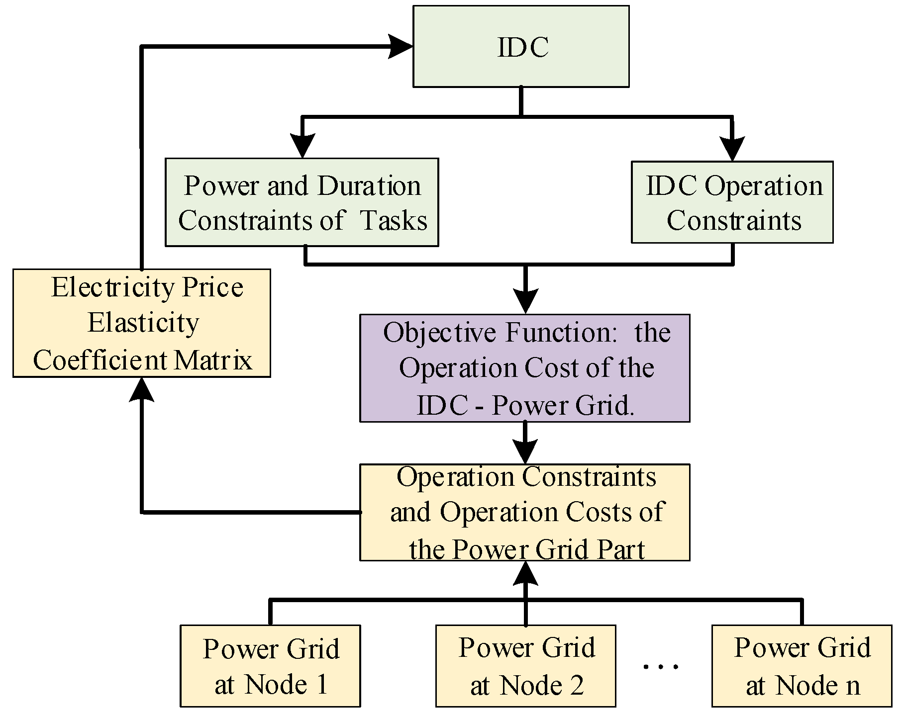
2.1. Two-Layer Optimization Model of IDC-Power Grid

Existing IDC modeling primarily falls into three categories: first, modeling based on device efficiency [15]; second, modeling based on factors influencing computation load handling [16,17,18]; and third, modeling based on computation load scheduling methods, which primarily involves incorporating load balancing algorithms from the computer field into energy consumption modeling [11,19].

This paper uses the time-of-use (TOU) price as the price signal of each area to guide the transfer of the computational task and derive the double-layer optimization model which is shown in Figure 1. The upper layer is for the dispatch to the IDC, and the lower model is for the power system dispatch. The object is the minimum of the total operational cost of the system of IDC and the power grid. The dispatch and TOU price of the computational load center are exchanged between the layers to iteratively find the optimal dispatch scheme [20].

The dispatch model of the IDC is at the upper layer. The objective function is the minimum operation cost of the IDC. The decision variables include the total electrical load (P_DC), the task number λ, and the operational state set I of the information transmission cables of the computational power clusters. The constraints include the upper and the lower limit of the computational power clusters, the maximum and the minimum number of the computational tasks, and the start and stop of the different equipment.

The dispatch model to each node of the power grid is at the lower layer. The objective function is to minimize the operating cost of the node power network. The decision variables include the start–stop states of each unit in the region and the output power p of each unit in the region. The constraints include power balance constraints, ramp-rate constraints, unit start–stop constraints, and the upper and lower limits of unit output constraints.

After the lower layer optimization results are processed to obtain the demand-side response power of the IDC, they are transmitted to the upper layer. The upper layer optimizes the power loads of data centers in each region according to the time-of-use electricity price and transmits them to the lower layer. After iteration, the final optimization results of the two-layer model are obtained.

2.2. IDC-Power System Model

2.2.1. Power System Model

In the bi-level model, the power grid dispatch model for each node aims to minimize the operation cost of the power grid. The constraints include power balance constraints of generating units, spinning reserve constraints, generating unit’s output constraints, etc. The details are as follows:

(1) Power balance constraints and spinning reserve constraints:

$$\left\{\begin{array}{c}{\displaystyle \sum _g\left(p_{g,t}+P_g^{\min }{u}_{g,t}\right)}+{\displaystyle \sum _w{p}_{w,t}}=D_t\\ {\displaystyle \sum _g{r}_{g,t}}\ge R_t\end{array}\right.$$

(1)

In Equation (1), p_g,t is the power output of unit g at time t that is higher than the minimum power output; $P_g^{\min }$ is the minimum power output of unit g; $p_{w,t}$ is the power output of the new energy unit at time t; D_t is the load demand of the system at time t; r_g,t is the spinning reserve capacity provided by unit g at time t; R_t is the spinning reserve capacity required by the system at time t; and u_g,t is the start–stop status of unit g, which is a 0–1 variable.

(2) Constraints on the output limits of generating units:

$$\left\{\begin{array}{c}{U}_g^0\left(P_g^0-P_g^{\min }\right)\le \left(P_g^{\max }-P_g^{\min }\right)U_g^0-\max \left\{\left(P_g^{\max }-S{D}_g\right),0\right\}\cdot w_g^1\\ p_{g,t}+r_{g,t}\le \left(P_g^{\max }-P_g^{\min }\right)u_{g,t}-\max \left\{\left(P_g^{\max }-S{U}_g\right),0\right\}\cdot v_{g,t}\\ p_{g,t}+r_{g,t}\le \left(P_g^{\max }-P_g^{\min }\right)u_{g,t}-\max \left\{\left(P_g^{\max }-S{D}_g\right),0\right\}\cdot w_{g,t+1}\end{array}\right.$$

(2)

In Equation (2), SU_g and SD_g represent the maximum ramp-up and ramp-down rates of unit g during start-up/shut-down, respectively, and are 0–1 variables; $P_g^{max}$ represents the maximum output of unit g; $P_g^0$ represents the initial output of unit g; $U_g^0$ represents the start-up/shut-down status of unit g at the initial moment, which is a 0–1 variable; v_g,t represents the start-up status of unit g at time t; w_g,t+1 represents the shut-down status of unit g at time t + 1; and $w_g^1$ represents the initial shut-down status of unit g, which are all 0–1 variables.

(3) Ramp rate constraints of generating units:

$$\left\{\begin{array}{c}{p}_g^1+r_g^1-U_g^0\left(P_g^0-P_g^{\min }\right)\le R{U}_g\\ U_g^0\left(P_g^0-P_g^{\min }\right)-p_g^1\le R{D}_g\\ p_{g,t}+r_{g,t}-p_{g,t-1}\le R{U}_g\\ p_{g,t-1}-p_{g,t}\le R{D}_g\end{array}\right.$$

(3)

In Equation (3), RU_g and RD_g, respectively, represent the maximum ramp rates of the unit during upward and downward ramping; p_g,t−1 is the power output of the unit that is higher than the minimum output at time; $r_g^1$ is the spinning reserve capacity provided by the unit at the initial moment; and $p_g^1$ is the power output of the unit at the initial moment.

(4) Constraints regarding the power of generating units, costs, start–stop statuses of generating units, and the output of new energy sources:

$$\left\{\begin{array}{l}{p}_{g,t}={\displaystyle \sum _l\left(P_g^l-P_g^1\right)}{\lambda }_{g,t}^l\\ c_{g,t}={\displaystyle \sum _l\left(C{P}_g^l-C{P}_g^1\right)}{\lambda }_{g,t}^l\\ u_{g,t}={\displaystyle \sum _l{\lambda }_{g,t}^l}\\ P_{w,t}^{\min }\le p_{w,t}\le P_{w,t}^{\max }\end{array}\right.$$

(4)

In Equation (4), $P_{w,t}^{\max }$ and $P_{w,t}^{\min }$, respectively, represent the maximum and minimum output of the new energy unit g at time t; p_g,t is the output of the new energy unit g at time t; ${\lambda }_{g,t}^l$ represents the power of unit g on the piecewise linearized output–cost function at time t; and c_g,t is the power generation cost of unit g when its output is higher than the minimum output at time t.

2.2.2. IDC Model

The tasks within the IDC can be divided into four types: reducible tasks, transferable tasks, shiftable tasks, and rigid tasks, each of which has different adjustment characteristics and features.

Shiftable tasks cannot be shut down during operation and their power remains constant. Rigid tasks are important loads that do not participate in scheduling, with a fixed load quantity, and will not change according to electricity prices, demands, or statuses. The characteristic of transferable tasks is that the total electricity consumption is fixed, but these tasks can be started and stopped at any time within a certain time range. This is manifested in that the starting time and usage frequency of the tasks can be adjusted, but the total usage duration and average power remain unchanged. Reducible tasks can have their power reduced or even be shut down during operation, but the usage time cannot be adjusted.

Based on the electricity consumption characteristics of IDC tasks, such as their start time, operational duration, power consumption, and frequency of use, IDC tasks can be classified into three categories based on their adjustability. Time-of-use (TOU) electricity prices act as pricing signals to encourage IDCs to adjust both the timing of their tasks and task volumes. Each category exhibits distinct adjustability features, as detailed in

Table 1. Assignment classification and adjustable electricity consumption features.

Assignment Type	Characteristic	Before	After	Assignment Number
reducible tasks	average power	pk	$p_k^{*}$	[m1 + 1, m2]
transferable tasks	startup time	tk	$t_k^{*}$	[m2 + 1, m3]
shiftable tasks	startup time	tk	$t_{k1}^{*}$…$t_{kn}^{*}$	[m3 + 1, m4]

.

Assume that there are D computing clusters in the IDC scheduled over T time periods. The operating cost of the computing clusters in the IDC consists of IT service costs, server startup costs, and task transmission costs. The scheduling model aims to minimize the operating cost of the IDC, and the constraints include the power constraints of the computing clusters, the constraints of non-interruptible tasks, etc. The details are as follows:

The IT service cost and its constraint, Equation (6), describe the upper and lower limit constraints of the power of the computing clusters that provide IT services:

$$\left\{\begin{array}{l}{C}_{d,t}^{IT}=c_{d,t}\cdot p_{d,t}\\ P_d^{\min }{\alpha }_{d,t}\le p_{d,t}\le P_d^{\max }{\alpha }_{d,t}\end{array}\right.$$

(5)

In Equation (5), $C_{d,t}^{IT}$ is the IT service cost of the d-th computing cluster at time t; c_d,t is the nodal electricity price of the d-th computing cluster at time t; p_d,t is the power of the d-th computing cluster at time t; $P_d^{\min }$ and $P_d^{\max }$ are, respectively, the minimum and maximum power values of the d-th computing cluster; and α_d,t is the operating status of the d-th computing cluster at time t, which is a 0–1 variable, where 1 represents the operating status and 0 represents the shutdown status.

Equation (6) describes the server startup cost of the computing cluster and the start–stop status constraints after the linearization of the computing cluster:

$$\left\{\begin{array}{l}{C}_{d,t}^{SU}=S{U}_d{y}_{d,t}\\ y_{d,t}-z_{d,t}=I_{d,t}-I_{d,t-1}\\ y_{d,t}\le 1-I_{d,t-1}\\ z_{d,t}\le I_{d,t-1}\\ 0\le y_{d,t}\le 1\\ 0\le z_{d,t}\le 1\end{array}\right.$$

(6)

In Equation (6), $C_{d,t}^{SU}$ is the server startup cost of the d-th computing cluster at time t; SU_d is the startup cost of the d-th computing cluster; and y_d,t and z_d,t, respectively, represent the startup and shutdown statuses of the d-th computing cluster at time t, which are 0–1 variables. For y_d,t, 1 indicates startup at this moment, and 0 indicates that there is no startup action at this moment.

For shiftable tasks, the IT service constraints are as follows, which include the constant power constraint and the continuity constraint of the task duration:

$$\left\{\begin{array}{l}{p}_{d,t}={\displaystyle \frac{{\lambda }_{d,t}}{{\lambda }_d^{\max }}}\cdot P_d^{\max }\\ T_{\mathrm{end}}-T_{\mathrm{start}}={\displaystyle \frac{{\displaystyle \sum _{t=1}^{T_{\mathrm{end}}-T_{\mathrm{start}}}t{p}_{d,t}}}{{\displaystyle \sum _{t=T_{\mathrm{start}}}^{T_{\mathrm{end}}}{\gamma }_d{\lambda }_{d,t}}}}\\ 0\le {\lambda }_{d,t}\le {\lambda }_d^{\max }\cdot I_{d,t}\\ T_{\mathrm{start}},T_{\mathrm{end}}\in T\end{array}\right.$$

(7)

In Equation (7), T_end and T_start, respectively, represent the task completion time node and the task start time node of the shiftable task; γ_d is the computing power load required for the d-th computing cluster to process a single task at time t.

For rigid tasks, the constraints of the IT services are as follows, including the quantity constraint of tasks to be processed and the constant power constraint:

$$\left\{\begin{array}{l}0\le {\lambda }_{d,t}\le {\lambda }_d^{\max }\cdot I_{d,t}\\ p_{d,t}={\displaystyle \frac{{\lambda }_{d,t}}{{\lambda }_d^{\max }}}\cdot P_d^{\max }\end{array}\right.$$

(8)

In Equation (8), λ_d,t is the number of tasks processed by the d-th computing cluster at time t; ${\lambda }_d^{\max }$ is the maximum number of tasks that the d-th computing cluster can process; and I_d,t is the task processing status, which is a 0–1 variable, where 1 represents the processing status and 0 represents the stopped status.

For transferable tasks, the IT service constraints are as follows, including the power constraint and the balance constraint of the number of transferable tasks:

$$\left\{\begin{array}{l}{\displaystyle \sum _{t=1}^T{I}_{d,t}}=H_d-R_S^d+R_R^d\\ {\displaystyle \sum _{t=1}^T{\displaystyle \sum _{d=1}^D{I}_{d,t}}}={\displaystyle \sum _{d=1}^D{H}_d}\\ p_{d,t}\le P_d^{\max }\cdot I_{d,t}\end{array}\right.$$

(9)

In Equation (9), $R_S^d$ is the number of hours of interruptible tasks transferred out from the d-th computing cluster; $R_R^d$ is the number of hours of interruptible tasks transferred to the d-th computing cluster; H_d is the initial number of hours of interruptible tasks that the d-th computing cluster needs to process; T is the scheduling time period; and D is the total number of computing clusters participating in the scheduling.

For reducible tasks, the IT service constraints are as follows, which include the continuity constraint of the task duration and the power constraint:

$$\left\{\begin{array}{l}{T}_{\mathrm{end}}-T_{\mathrm{start}}={\displaystyle \frac{{\displaystyle \sum _{t=1}^{T_{\mathrm{end}}-T_{\mathrm{start}}}t{p}_{d,t}}}{{\displaystyle \sum _{t=T_{\mathrm{start}}}^{T_{\mathrm{end}}}{\gamma }_d{\lambda }_{d,t}}}}\\ 0\le p_{d,t}\le P_{d,\max }\cdot I_{d,t}\end{array}\right.$$

(10)

Equation (11) describes the task transmission cost of the computing cluster:

$$\left\{\begin{array}{l}{C}_{d,t}^T=c_{d,t}\cdot p_{d,t}^T\\ p_{d,t}^T={\displaystyle \sum _{m=1}^{N_m}{P}_m\cdot {\beta }_{m,d,t}}\end{array}\right.$$

(11)

In Equation (11), $C_{d,t}^T$ is the data transmission cost of the d-th computing cluster at time t; $p_{d,t}^T$ is the power of the tasks transmitted by the d-th computing cluster at time t, P_m is the power consumed on a single cable; and β_m,d,t is the task incoming status of the m-th cable on the d-th computing cluster at time t, which is a 0–1 variable, where 1 represents the incoming status and 0 represents the stopped transmission status.

2.2.3. Joint Scheduling Model Objective Function

Equation (12) defines the total system cost of coordinated optimization scheduling to the IDC and the power grid. It has two components: (1) the operational cost of the IDC, including the IT service cost, server startup cost, and task transmission cost, and (2) the operational cost of the grid, including the startup and shutdown cost of generation units and the operation cost of generations.

$$\min {\displaystyle \sum _{t=1}^T{\displaystyle \sum _{d=1}^D\left(C_{d,t}^{IT}+C_{d,t}^{SU}+C_{d,t}^T\right)}}+{\displaystyle \sum _g{\displaystyle \sum _t\left(c_{g,t}+C{P}_g^1\cdot u_{g,t}\right)}}$$

(12)

2.2.4. Joint Scheduling Model Operating Constraints

The IDC-power grid joint scheduling model needs to comply with all the operating constraints in Equations (1)–(11).

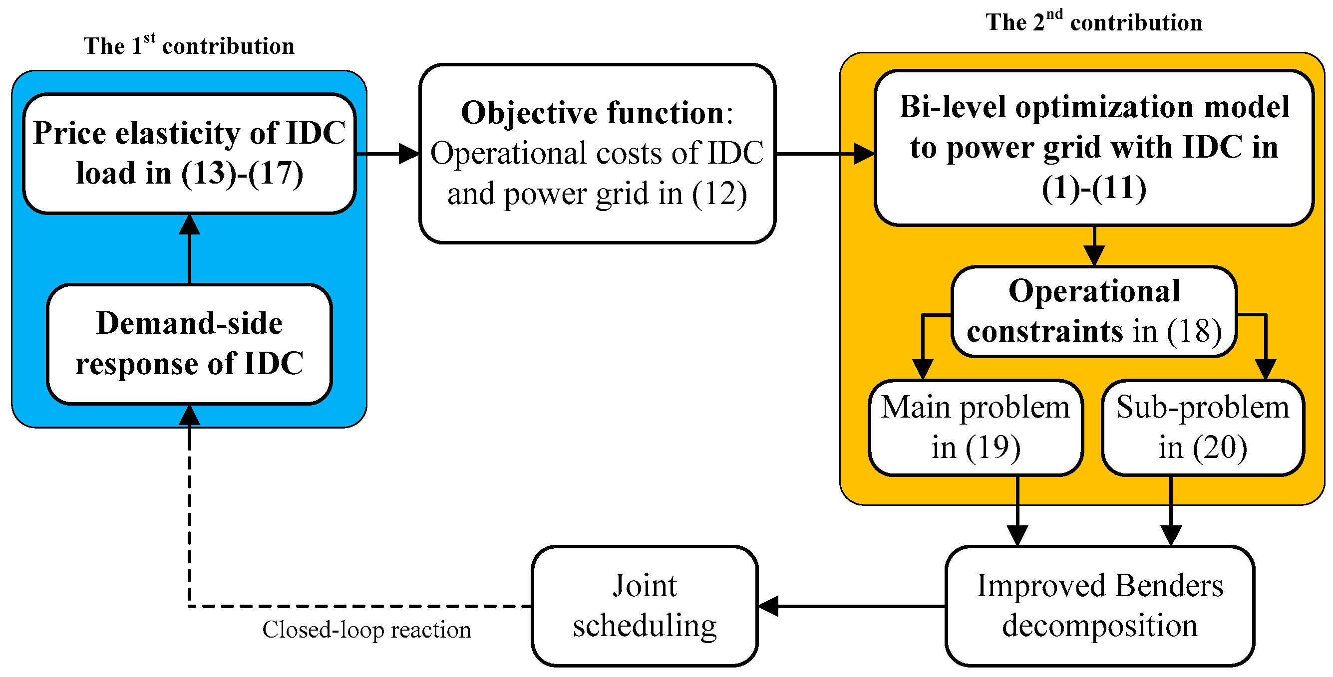
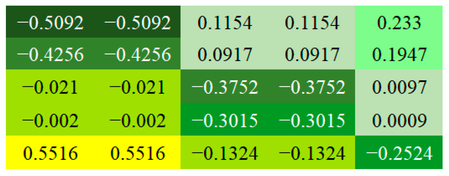
2.3. Solution of the Electricity Price Elasticity Coefficient Matrix of the IDC

For the demand-side response of time-of-use electricity prices, the electricity consumption periods are usually divided into three types of electricity load periods: peak, flat, and valley. Accordingly, the demand-side response model of the time-of-use electricity prices for the IDC loads participating in the response can be expressed as

$$\left[\begin{array}{c}{P}^{\mathrm{p}}\\ P^{\mathrm{f}}\\ P^{\mathrm{v}}\end{array}\right]=\mathrm{diag}(P^{\mathrm{p},0},P^{\mathrm{f},0},P^{\mathrm{v},0})\mathit{E}\left[\begin{array}{c}{\displaystyle \frac{\Delta {\lambda }^{\mathrm{p}}}{{\lambda }^{\mathrm{p},0}}}\\ {\displaystyle \frac{\Delta {\lambda }^{\mathrm{f}}}{{\lambda }^{\mathrm{f},0}}}\\ {\displaystyle \frac{\Delta {\lambda }^{\mathrm{v}}}{{\lambda }^{\mathrm{v},0}}}\end{array}\right]+\left[\begin{array}{c}{P}^{\mathrm{p},0}\\ P^{\mathrm{f},0}\\ P^{\mathrm{v},0}\end{array}\right]$$

(13)

In Equation (13), P^p,0, P^f,0, and P^v,0 and P^p, P^f, and P^v represent the total electrical loads of the electricity-consuming users participating in the demand-side response during the peak, flat, and valley electricity load periods before and after the introduction of the time-of-use electricity price demand-side response, respectively; E is the demand elasticity matrix of the electricity-consuming users participating in the response; Δλ^p, Δλ^f, and Δλ^v are the changes in the system electricity prices during the peak, flat, and valley electricity load periods after the introduction of the time-of-use electricity price demand-side response; and λ^p,0, λ^f,0, and λ^v,0 are the system electricity prices during the peak, flat, and valley electricity load periods before the introduction of the time-of-use electricity price demand-side response. For the same type of electricity-consuming users, λ^p,0, λ^f,0, and λ^v,0 are often the same value and can be expressed as the basic electricity price λ⁰.

Divide the electricity consumption periods of the IDC task loads into three types of electricity load periods: peak, flat, and valley. The electricity price elasticity matrix of the IDC task loads participating in the response can be expressed as

$$\mathit{E}=\left[\begin{array}{ccc}{e}^{\mathrm{pp}}& e^{\mathrm{pf}}& e^{\mathrm{pv}}\\ e^{\mathrm{fp}}& e^{\mathrm{ff}}& e^{\mathrm{fv}}\\ e^{\mathrm{vp}}& e^{\mathrm{vf}}& e^{\mathrm{vv}}\end{array}\right]$$

(14)

In Equation (14), eⁱⁱ is the self-elasticity coefficient; e^ij is the cross-elasticity coefficient.

The price elasticity of the demand coefficient can effectively represent the sensitivity of the electricity consumption demand of electricity load users participating in the demand-side response of time-of-use electricity prices to the changes in electricity prices, that is, the price elasticity of the demand coefficient:

$$e^{ij}=\left(\Delta P^i/P^{i,0}\right)/\left(\Delta {\lambda }^j/{\lambda }^{j,0}\right)$$

(15)

In Equation (15), ΔPⁱ and Δλ^j are, respectively, the change in the total electricity load participating in the response in the system during the i-th scheduling period and the change in the electricity price during the j-th scheduling period after the demand-side response of the time-of-use electricity price; P^i,0 and Δλ^j,0 are, respectively, the total electricity load participating in the response in the system during the i-th scheduling period and the electricity price during the j-th scheduling period before the demand-side response of the time-of-use electricity price.

As shown in Figure 2, classify the tasks of the IDC according to their characteristics, study the responses of different load tasks to electricity prices, respectively, and construct the electricity price elasticity coefficient matrix of the IDC considering the load characteristics of different tasks.

If the task is a transferable task, since there is no transfer of electricity consumption, it only affects the self-elasticity coefficient. If it is a shiftable task, the electricity consumption is transferred from period i to period j. As the amount of electricity transfer is caused by the change in the electricity price difference between the two periods, it only affects the cross-elasticity coefficient. If it is a transferable task, the electricity consumption can be transferred from moment i to multiple moments, which is represented by the set T = (t₁, t₂…, t_n). Then, the cross-elasticity coefficients related to the set T will all be affected.

Based on the elasticity coefficient matrix, calculate the changes in electricity demand for the three types of tasks (shiftable tasks, transferable tasks, and reducible tasks) of the d-th computing cluster according to the original electricity consumption, initial electricity price, and the change in electricity price. Then, incorporate these demand changes into the optimal scheduling calculation to adjust the power output of the IDC.

$${\left[\Delta P_{\mathrm{d}1} \Delta P_{\mathrm{d}2}\cdots \Delta P_{\mathrm{dn}}\right]}^{\mathrm{T}}={\left[P_{\mathrm{d}1} P_{\mathrm{d}2}\cdots P_{\mathrm{dn}}\right]}^{\mathrm{T}}{\mathit{E}}_{\mathrm{d}}{\left[{\displaystyle \frac{\Delta {\lambda }_{\mathrm{d}1}}{{\lambda }_{\mathrm{d}1}}}{\displaystyle \frac{\Delta {\lambda }_{\mathrm{d}2}}{{\lambda }_{\mathrm{d}2}}}\cdots {\displaystyle \frac{\Delta {\lambda }_{\mathrm{d}n}}{{\lambda }_{\mathrm{d}n}}}\right]}^{\mathrm{T}}$$

(16)

In Equation (16), ΔP_d1, ΔP_d2, and ΔP_dn represent the changes in electricity demand at the first moment, the second moment, and the n-th moment, respectively, for the d-th computing power cluster; P_d1, P_d2, and P_dn represent the original electricity demands at the first moment, the second moment, and the n-th moment, respectively, for the d-th computing power cluster; Δλ_d1, Δλ_d2, and Δλ_dn represent the changes in electricity prices at the first moment, the second moment, and the n-th moment, respectively, for the d-th computing power cluster; λ_d1, λ_d2, and λ_dn represent the original electricity prices at the first moment, the second moment, and the n-th moment, respectively, for the d-th computing power cluster; and E_d is the time-of-use electricity price elasticity coefficient matrix of the d-th computing power cluster.

Based on Equation (16), calculate the change in task electricity demand of the d-th computing cluster. Expand Equation (16) to other computing clusters to calculate the changes in electricity demand of the remaining computing clusters. In this way, obtain the changes in electricity demand of the IDC at each moment resulting from the changes in electricity prices.

$${\left[\Delta P_1 \Delta P_2\cdots \Delta P_{\mathrm{n}}\right]}^{\mathrm{T}}={\left[{\displaystyle \sum _{d=1}^D\Delta P_{d1}} {\displaystyle \sum _{d=1}^D\Delta P_{d2}}\cdots {\displaystyle \sum _{d=1}^D\Delta P_{d\mathrm{n}}}\right]}^{\mathrm{T}}$$

(17)

In Equation (17), ΔP₁, ΔP₂, and ΔP_n are, respectively, the changes in the electricity demand of the IDC at the first moment, the second moment, and the n-th moment.

Add the change in electricity demand calculated by Equation (17) into the IDC-power grid distributed optimal scheduling method. Adjust the solution processes of the main problem and the sub-problems, respectively, according to the demand response quantity, so as to obtain the coordinated optimal scheduling result of the IDC and the power grid that takes into account the influence of electricity prices.

3. Distributed Solving Method

During the solving process of the joint scheduling problem, both the IDC and the power network pursue overall economic optimality, while also having a need for privacy protection. Information such as user demand characteristics and planning results is often difficult to share. Therefore, a distributed solution method based on enhanced Benders decomposition is adopted [21,22,23].

3.1. Enhanced Benders Decomposition

Enhanced Benders decomposition is suitable for non-convex problems with a discrete 0–1 variable. Ref. [24] gives a detailed derivation of this algorithm and proves its effectiveness. To solve the problem of unified planning of the power system with the IDC, the improved Benders decomposition is given as follows.

Based on the joint scheduling model of the IDC-power system, the original problem of the enhanced Benders decomposition method for solving the optimal scheduling of the system is as follows:

$$\left\{\begin{array}{l}\underset{\mathit{x},\mathit{y},{\mathit{x}}_{\mathit{i}}^{\mathbf{\prime }},{\mathit{y}}_{\mathit{i}}^{\mathbf{\prime }},\mathit{m}}{\min } (\mathit{gy}+{\displaystyle \sum _{i\in N}{\mathit{h}}_{\mathit{i}}{\mathit{y}}_i^{\mathbf{\prime }}})\\ \mathrm{s}.\mathrm{t}. \mathit{Ax}+\mathit{By}+\mathit{Cm}⩾\mathit{e}\\ {\mathit{D}}_{\mathit{i}}\mathit{m}+{\mathit{E}}_{\mathit{i}}{\mathit{x}}_{\mathit{i}}^{\mathbf{\prime }}+{\mathit{F}}_{\mathit{i}}{\mathit{y}}_i^{\mathbf{\prime }}⩾{\mathit{f}}_i,\hspace{1em}\forall i\in N\\ \mathit{x},{\mathit{x}}_{\mathit{i}}^{\mathbf{\prime }}\in \{0,1\},\hspace{1em}\forall i\in N\end{array}\right.$$

(18)

In Equation (18), x is a vector composed of 0–1 variables related to the IDC part; ${\mathit{x}}_{\mathit{i}}^{\mathbf{\prime }}$ is a vector composed of 0–1 variables related to the power grid part; y is a vector composed of continuous variables related to the IDC part; ${\mathit{y}}_{\mathit{i}}^{\mathbf{\prime }}$ is a vector composed of continuous variables related to the power grid part; m is a vector composed of coupling variables between the IDC and the power grid; $\mathit{Ax}+\mathit{By}+\mathit{Cm}⩾\mathit{e}$ represents the constraint conditions of the IDC; ${\mathit{D}}_{\mathit{i}}\mathit{m}+{\mathit{E}}_{\mathit{i}}{\mathit{x}}_{\mathit{i}}^{\mathbf{\prime }}+{\mathit{F}}_{\mathit{i}}{\mathit{y}}_i^{\mathbf{\prime }}⩾{\mathit{f}}_i$ represents the constraint conditions of the power grid; A, B, C, D_i, E_i, and F_i are constant-term matrices, respectively; and e, f_i, g, and h_i are constant-coefficient vectors, respectively.

The original problem may be divided into a master problem and N subproblems. Based on the solution of the master problem, the feasibility and optimality of each subproblem are checked. The master problem is planning the transferrable task of the IDC, i.e.,

$$\left\{\begin{array}{l}\underset{{\mathit{x}}^{\mathbf{\prime }},{\mathit{y}}^{\mathbf{\prime }},{\mathit{m}}^{\mathbf{\prime }},{\theta }_i}{\min }({\mathit{g}}^{\mathbf{\prime }}{\mathit{y}}^{\mathbf{\prime }}+{\displaystyle \sum _{i\in N}{\theta }_i})\\ \mathrm{s}.\mathrm{t}. {\mathit{A}}^{\mathbf{\prime }}{\mathit{x}}^{\mathbf{\prime }}+{\mathit{B}}^{\mathbf{\prime }}{\mathit{y}}^{\mathbf{\prime }}\ge {\mathit{e}}^{\mathbf{\prime }}\\ {\theta }_i\ge 0,\hspace{1em}\forall i\in N\\ {\mathit{x}}^{\mathbf{\prime }}\in \{0,1\}\end{array}\right.$$

(19)

In Equation (19), θ_i is the relevant lower limit costs determined by the master problem; ${\mathit{A}}^{\mathbf{\prime }}$ and ${\mathit{B}}^{\mathbf{\prime }}$ are constant-term matrices; ${\mathit{e}}^{\mathbf{\prime }}$ and ${\mathit{g}}^{\mathbf{\prime }}$ are constant-coefficient vectors; ${\mathit{x}}^{\mathbf{\prime }}$ is a vector composed of 0–1 variables related to transferable loads; and ${\mathit{y}}^{\mathbf{\prime }}$ is a vector composed of continuous variables related to transferable loads.

The subproblems consider the coordinated dispatch and planning of the power system with the IDC but exclude the transferrable load. The feasibility and optimality of the subproblems may be proved simultaneously.

$$\left\{\begin{array}{l}\underset{\mathit{z},\mathit{u},{\mathit{z}}_{\mathit{i}}^{\mathbf{\prime }},{\mathit{u}}_{\mathit{i}}^{\mathbf{\prime }},\mathit{m}}{\min } (\mathit{gu}+{\displaystyle \sum _{i\in N}{\mathit{h}}_{\mathit{i}}{\mathit{u}}_{\mathit{i}}^{\mathbf{\prime }}})\\ \mathrm{s}.\mathrm{t}. \mathit{Hz}+\mathit{Iu}+\mathit{Jm}⩾\mathit{a}\\ {\mathit{K}}_{\mathit{i}}\mathit{m}+{\mathit{L}}_{\mathit{i}}{\mathit{z}}_{\mathit{i}}^{\mathbf{\prime }}+{\mathit{M}}_{\mathit{i}}{\mathit{u}}_{\mathit{i}}^{\mathbf{\prime }}⩾{\mathit{b}}_i,\hspace{1em}\forall i\in N\\ \mathit{z},{\mathit{z}}_{\mathit{i}}^{\mathbf{\prime }}\in \{0,1\},\hspace{1em}\forall i\in N\end{array}\right.$$

(20)

In Equation (20), z is a vector composed of 0–1 variables related to the IDC excluding transferable loads; ${\mathit{z}}_{\mathit{i}}^{\mathbf{\prime }}$ is a vector composed of 0–1 variables related to the power grid part; u is a vector composed of continuous variables related to the IDC excluding transferable loads; ${\mathit{u}}_{\mathit{i}}^{\mathbf{\prime }}$ is a vector composed of continuous variables related to the power grid part; $\mathit{Hz}+\mathit{Iu}+\mathit{Jm}⩾\mathit{a}$ represents the constraint conditions of the IDC excluding transferable loads; ${\mathit{K}}_{\mathit{i}}\mathit{m}+{\mathit{L}}_{\mathit{i}}{\mathit{z}}_{\mathit{i}}^{\mathbf{\prime }}+{\mathit{M}}_{\mathit{i}}{\mathit{u}}_{\mathit{i}}^{\mathbf{\prime }}⩾{\mathit{b}}_i$ represents the constraint conditions of the power grid part; H, I, J, K_i, L_i, M_i are constant-term matrices, respectively; and a, b_i, g and h_i are constant-coefficient vectors, respectively.

Since there is a discrete 0–1 variable, one can not generate the Benders cut through the duality. The improved Benders decomposition proposes an auxiliary variable ${\tilde{x}}^{\mathbf{\prime }}$ and the min/max equality for approximate duality to derive the unified dual subproblem $F_{D,i}^{*}$,

$$F_{D,i}^{*}=\underset{({\mathit{J}}_{\mathit{i}},{\mathit{K}}_{\mathit{i}},{\mathit{L}}_{\mathit{i}})\in {\mathit{N}}_{\mathit{i}}\cup {\mathit{M}}_{\mathit{i}}}{\max }\left[{({\mathit{f}}_i^{\mathbf{\prime }}-{\mathit{D}}_i^{\mathbf{\prime }}{\overline{\mathit{m}}}^{\mathbf{\prime }})}^T{\mathit{J}}_i+{\mathbf{1}}^T{\mathit{L}}_i\right]$$

(21)

When its optimal solution is equal to 0, the current solution of the master problem is considered to meet the requirements of feasibility and optimality. Otherwise, to exclude the current solution, a Benders cut should be added to the master problem:

$${\left({\mathit{f}}_i^{\mathbf{\prime }}-{\mathit{D}}_i^{\mathbf{\prime }}{\overline{\mathit{m}}}^{\mathbf{\prime }}\right)}^T{\overline{\mathit{J}}}_{\mathit{i}}+1^T{\overline{\mathit{L}}}_{\mathit{i}}\le 0$$

(22)

In Equation (22), ${\overline{\mathit{J}}}_{\mathit{i}}$ and ${\overline{\mathit{L}}}_{\mathit{i}}$ are the optimal solutions of the variables in the unified dual sub-problem.

Compared with the traditional Benders decomposition, the approximate duality yields the dual gap between the unified dual subproblem and the unified original subproblem; thus, (22) can not exclude all the non-feasible solutions and the non-optimal solutions. To eliminate the gap, after the unified dual subproblem, the feasibility restore subproblem has to be solved.

$$\left\{\begin{array}{l}{F}_{F,i}^{*}=\underset{{\mathit{m}}^{\mathbf{\prime }},{\mathit{x}}_{\mathit{i}}^{\mathbf{\prime }},{\mathit{y}}_i^{\mathbf{\prime }}}{\min }{\Delta }_i\left({\mathit{m}}^{\mathbf{\prime }},{\overline{\mathit{m}}}^{\mathbf{\prime }}\right)\\ \mathrm{s}.\mathrm{t}. {\mathit{D}}_{\mathit{i}}^{\mathbf{\prime }}{\mathit{m}}^{\mathbf{\prime }}+{\mathit{E}}_{\mathit{i}}{\mathit{x}}_{\mathit{i}}^{\mathbf{\prime }}+{\mathit{F}}_{\mathit{i}}{\mathit{y}}_{\mathit{i}}^{\mathbf{\prime }}\ge {\mathit{f}}_i^{\mathbf{\prime }}\\ {\mathit{x}}_{\mathit{i}}^{\mathbf{\prime }}\in \left\{0,1\right\}\end{array}\right.$$

(23)

In Equation (23), $F_{F,i}^{*}$ is the objective function value; ${\Delta }_i\left({\mathit{m}}^{\mathbf{\prime }},{\overline{\mathit{m}}}^{\mathbf{\prime }}\right)$ represents the feasibility deviation between ${\overline{\mathit{m}}}^{\mathbf{\prime }}$ and any ${\mathit{m}}^{\mathbf{\prime }}$ within the feasible region.

By solving Equation (23), when $F_{F,i}^{*}$ is greater than zero, the Benders cut shown in Equation (24) can be added to the master problem to exclude other non-optimal solutions:

$$\left\{\begin{array}{l}{\Delta }_i({\mathit{m}}^{\mathbf{\prime }},{\overline{\mathit{m}}}^{\mathbf{\prime }})\ge F_{F,i}^{*}\\ \Delta ({\mathit{m}}^{\mathbf{\prime }},{\overline{\mathit{m}}}^{\mathbf{\prime }})={\displaystyle \sum _n{o}_n}/{\omega }_n\\ o_n=|m_n^{\mathbf{\prime }}-{\overline{m}}_n^{\mathbf{\prime }}|\\ {\omega }_n={\left\{\begin{array}{ll}\left|{\overline{m}}_n^{\mathbf{\prime }}\right|,\hfill & \left|{\overline{m}}_n^{\mathbf{\prime }}\right|>0\hfill \\ \tau ,\hfill & \left|{\overline{m}}_n^{\mathbf{\prime }}\right|=0\hfill \end{array}\right.}_n\end{array}\right.$$

(24)

In Equation (24), o_n is the absolute deviation; ω_n is the normalization factor; $m_n^{\mathbf{\prime }}$, ${\overline{m}}_n^{\mathbf{\prime }}$ are specific elements in ${\mathit{m}}^{\mathbf{\prime }}$, ${\overline{\mathit{m}}}^{\mathbf{\prime }}$, respectively; and τ is a sufficiently small positive number.

3.2. Distributed Solution Process

Based on the master problem and the subproblems given in Section 3.1, the improved Benders decomposition is illustrated in Figure 3. At first, the master problem for the transferrable load is solved, and the solution is sent to the subproblems. Then, each subproblem is solved to generate the Benders cut. The process converges when the solution of the master problem does not change.

3.3. Discussion

(1) The price elasticity is related to the time-of-use electricity price and quantified with historical load-price data. But it changes with the time instead of being constant; hence, the price-elasticity coefficient matrix is to be checked and updated with time, especially when the load components and characteristics change notably.

(2) The time-of-use electricity price in this paper does not change with the system conditions. However, the power grid may change the time-of-use time curve to provide better service to the IDC while not increasing the burden of the peak-load scheduling.

(3) This paper optimizes one IDC with several load components with different responses to the change in electricity price. With increasing capacity, the IDCs may be located at different locations; thus, they may be optimized in a coordinated manner. Furthermore, if the distance of the IDCs is large enough, the peak–valley loads of the power grids occur at different times. Such spatial feature of multiple IDCs may be applied to reduce the cost of the power grid with the IDCs.

Therefore, the optimal scheduling method for IDC loads considering the response of computing power tasks proposed in this paper provides an effective approach for the optimal scheduling of the IDC-power system. In the future, online optimal scheduling of IDC loads will be taken as a key research direction.

4. Case Analysis

To verify the effectiveness of the models and algorithms proposed in this paper, this section conducts a case-based simulation test on the IDC-power system. The simulation test is carried out on a computer equipped with an Intel i5-12400 CPU and 16 GB of RAM.

System Case and Analysis

The test system consists of 10 generators and 39 nodes. A 1.5 MW wind farm is connected to Node 9, and an IDC is connected to Node 14. The topological structure diagram of the system is shown in Figure 4. Here, G represents a generator, and DFIG represents a wind farm. The DFIG parameters refer to Refs. [25,26,27,28].

In optimal scheduling considering the demand-side response of IDCs, if the uncertain factors are set as fixed parameters and optimal scheduling is carried out based on a single typical day of an IDC, the result lacks rationality. However, if the annual cycle is taken as the research period and optimal scheduling is carried out according to the annual load curve of an IDC, although theoretically it can improve the accuracy of the optimal scheduling result, it is not feasible in actual operation. Both the simulation time and the computational difficulty will increase, and it is difficult to ensure that an effective global optimal solution can be obtained. Therefore, it is necessary to carry out scenario reductions and analyses with representative IDC load curves to make the optimal scheduling scheme more efficient and reasonable. The daily load curves of multiple IDCs are reduced to a limited number of daily load curves while maintaining time continuity.

The scenario reduction in the IDC load curves is carried out based on the K-means clustering algorithm, and typical daily load curves are screened out for the next step of analysis.

The K-means algorithm can divide the feature matrix of samples into k non-overlapping clusters. According to empirical values, the number of clusters is generally between 3 and 7. In this paper, k is set from 1 to 10 to determine the best number of clusters in the clustering and observe the change in the sum of squared errors. SSE_k represents the error when all samples are clustered into k classes. The optimal number of clusters is judged according to the value of SSE_k:

$$SS{E}_k={\displaystyle \sum _{i=1}^k{\displaystyle \sum _{p\in C_i}|p-m_i{|}^2}}$$

(25)

In Equation (25), C_i is the i-th cluster; p is the sample point in C_i; and m_i is the centroid of C_i, that is, the mean value of all samples in C_i.

Selecting the daily load data of IDCs in 2024 for analysis, the K-means algorithm was employed to cluster the typical daily load patterns of IDCs.

As shown in Figure 5, the analysis resulted in the identification of five distinct categories of typical daily load curves for IDCs. The daily load curve with a maximum load was selected for simulation analysis of joint optimization and scheduling between the IDC and power grid. The simulation was conducted with a time step of 1 h.

As shown in Figure 6, there is a significant difference in the wind curtailment of the system between the cases of separate scheduling and joint scheduling.

In the case of separate scheduling of the IDC-power grid, the wind curtailment of the system is 9.08 MW. However, under the joint optimal scheduling of the IDC-power grid, the wind curtailment is only 0.37 MW. Considering the adjustability of the IDC computing power tasks, by adjusting the working time and task volume of the delay-tolerant tasks, the flexibility of the system is improved, which provides room for new energy consumption. As a result, the wind curtailment is reduced by 8.71 MW, and the operating cost of the power grid is correspondingly reduced.

Figure 7 shows the time-of-use electricity pricing mechanism in the region, which adopts peak–valley–flat electricity prices. The time periods of the time-of-use electricity price are dynamically adjusted according to seasons. The peak periods are from 8:00 to 11:00 and from 16:00 to 21:00, the off-peak period is from 23:00 to 8:00 the next day, and the flat periods are from 11:00 to 16:00 and from 21:00 to 23:00.

In the separate scheduling of the IDC-power grid, the IDC does not have flexible adjustment capabilities, and all tasks are regarded as delay-sensitive tasks. However, in the joint optimal scheduling of the IDC-power grid, the adjustability of delay-tolerant tasks is taken into account, and the time-of-use electricity price is used as a signal to guide the transfer of computing power tasks.

As shown in Figure 8, the computing tasks of the IDC change in terms of computing time periods and task power under the influence of electricity price signals. The delay-tolerant computing power tasks of the IDC migrate from peak electricity consumption periods to off-peak periods. This not only reduces the operating cost but also achieves the effect of new energy consumption.

In the case of separate scheduling of the IDC-power grid, the task load of the computing center cannot participate in demand-side response, and the load curve is relatively smooth. However, in the case of joint optimal scheduling of the IDC-power grid, since the delay-tolerant tasks are adjusted to other time periods, the electricity consumption load of the IDC during peak electricity consumption periods is reduced, playing a role in electricity load balancing.

Based on IDC historical load data, the method proposed in this paper can be used to calculate the electricity price elasticity coefficient matrix heatmap, as shown in Figure 9.

In the time-of-use electricity pricing periods, groups 1–2 are designated as peak periods, groups 3–4 as flat periods, and period 5 as off-peak periods. The self-elasticity coefficients and cross-elasticity coefficients between different periods are, respectively, calculated. Based on the electricity price elasticity coefficient matrix of IDCs, the demand response quantity of the IDC is calculated.

During the morning electricity peak (from 8:00 to 11:00) and the evening electricity peak (from 16:00 to 21:00), compared with separate scheduling, the IDC load under joint optimal scheduling is reduced by a total of 8.18 MW. Transferring the computing power load from the peak-price periods to the off-peak-price periods correspondingly reduces the operating cost of the IDC.

As can be seen from

Table 2. Cost comparison of system in different dispatch models.

Cost/$	Individual Optimization [B1–B2]	Branch and Bound [B3–B5]	Joint Optimization in This Paper
operation cost of power grid	11,389.66	11,078.46 ↓	10,965.94 ↓
operation cost of IDC	5888.25	5518.71 ↓	5040.95 ↓
total cost	17,277.91	16,597.17 ↓	16,006.89 ↓

, compared with the separate optimal scheduling of the IDC-power grid, after the joint optimal scheduling of the IDC-power grid, the computing power cost of the system is reduced by USD 843.52, the operating cost of the power grid is reduced by USD 423.72, and the total cost is reduced by USD 1267.25. Using the time-of-use electricity price as a signal to guide the change in the working time of the delay-tolerant load in the computing power center can not only contribute to the consumption of new energy output but also play a role in peak shaving and valley filling. It reduces the operating cost of the computing power center and promotes the consumption of new energy.

The enhanced Benders decomposition method is used to solve the joint optimal scheduling problem of the IDC-power system. The convergence curve of the algorithm is shown in Figure 10.

The convergence error ε is defined as $\epsilon =\left|C_1-C_2\right|/C_2$. C₁ is the optimal value of the joint optimal scheduling of the IDC-power grid based on the Benders decomposition method, and C₂ is the optimal value of the centralized joint optimal scheduling of the IDC-power grid. When the error value is 1, it can be considered that the sub-problem of the joint scheduling system is infeasible. When the error approaches 0, it indicates that the optimal value of the joint optimal scheduling of the IDC-power grid based on the Benders decomposition method is almost the same as that of the centralized method, which proves the effectiveness of the Benders decomposition method. When the threshold is set to 0.02, the Benders decomposition method approaches convergence after 110 iterations, taking 0.62 s.

To validate the robustness of the joint optimization model proposed in this paper, different daily load curves of the IDC are applied, with the results shown in Figure 11. It is found that the method proposed in this paper can effectively shift adjustable loads of IDC from peak to off-peak hours and reduce the operating cost of the IDC.

There are significant differences in computational performance between the joint optimal scheduling of the IDC-power grid based on the Benders decomposition method and the centralized joint optimal scheduling of the IDC-power grid. The details are shown in

Table 3. Computation performance comparison of system.

Type	Iteration	Time (s)
Centralized algorithm	1	0.05
Benders	112	0.62

.

In centralized optimal scheduling, all the information of the joint scheduling system is required, and all the constraints of the joint scheduling system need to be considered. In the IDC-power grid joint optimal scheduling based on the Benders decomposition method, the privacy of different entities is protected through information such as feasible cutting planes and optimal cutting planes.

5. Conclusions

Based on the establishment of a two-layer optimal scheduling model for the IDC-power grid, this paper proposes an optimal scheduling method for IDC loads considering the response of computing power tasks. The main work is as follows:

(1)

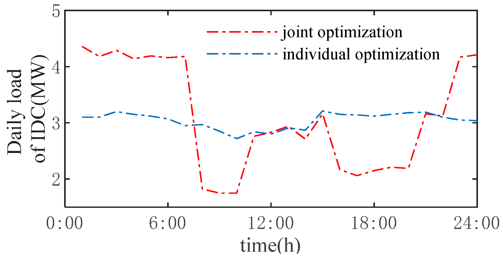
The IDC-power grid bi-level optimization model proposed in this paper can effectively express the collaborative optimization relationship between the two entities, achieving optimized planning while ensuring reasonable economic benefits for both systems. Compared with individual optimization, the proposed optimization model can reduce the operational costs of IDC and power grid systems by 7.356%.

(2)

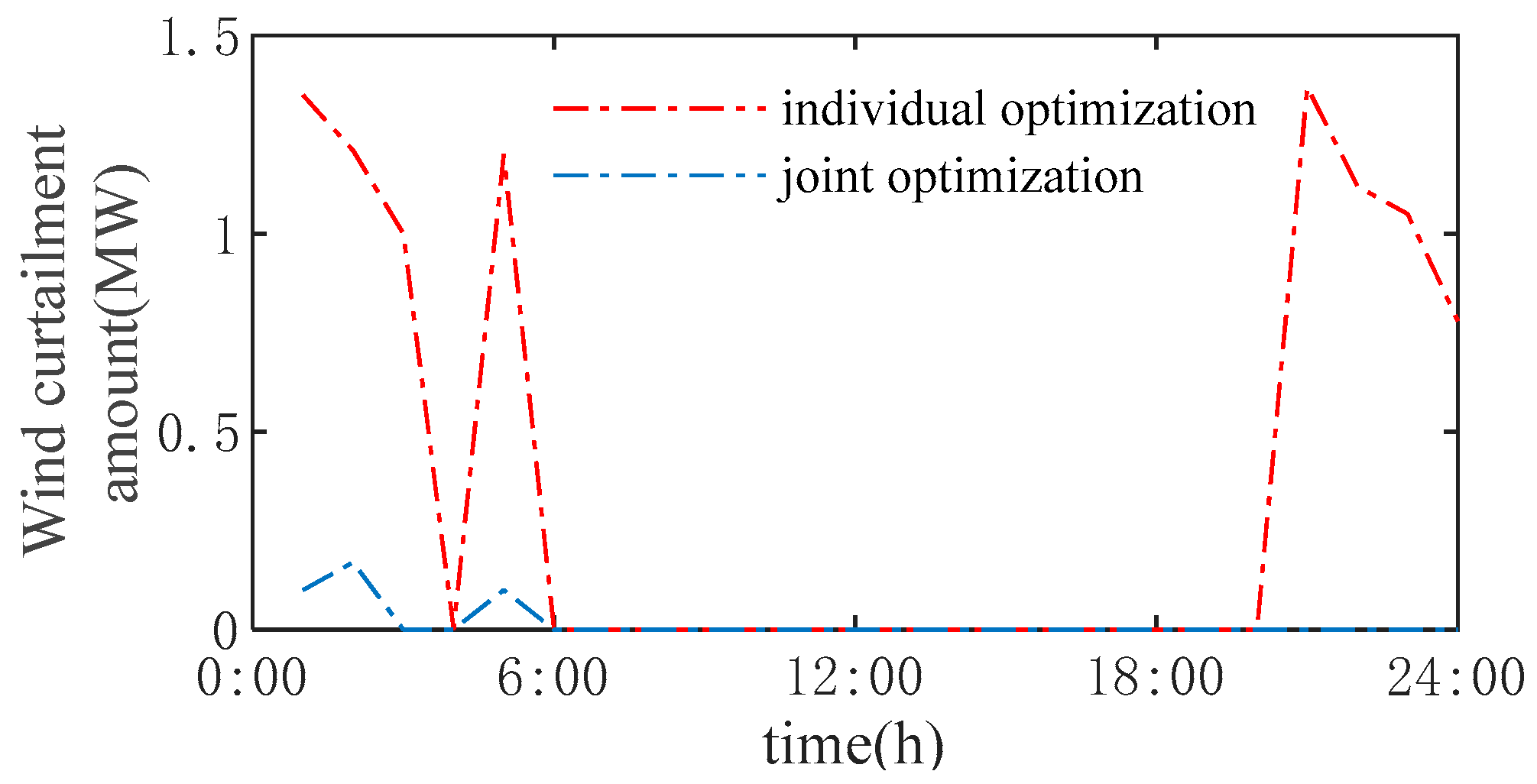
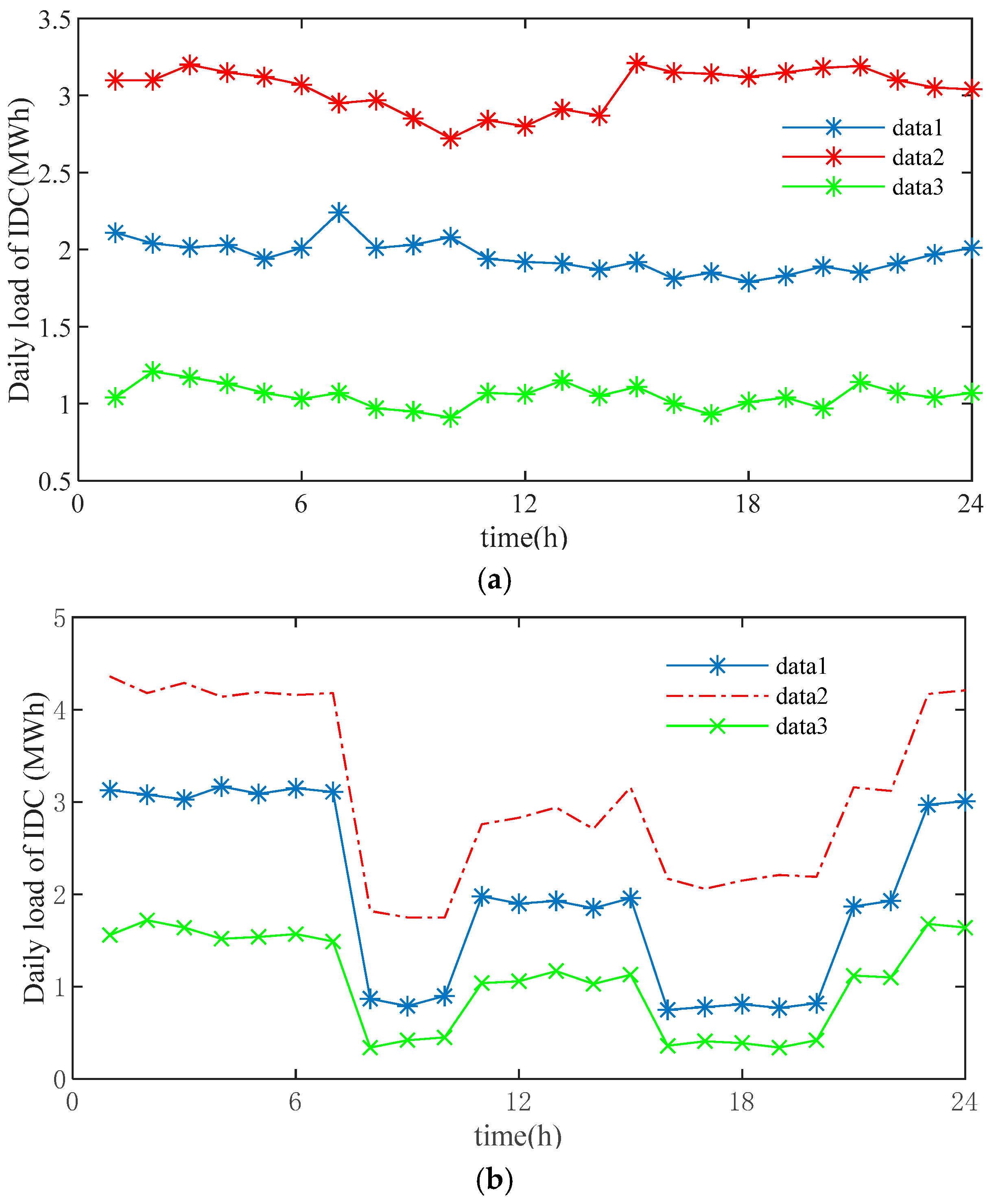
The time-of-use electricity price can guide IDC to adjust computing task scheduling strategies. With the adjustable characteristics of computing tasks, the IDC can participate in demand-side response. This mechanism facilitates peak shaving and valley filling in power systems while enhancing renewable energy integration.

(3)

A 39-node distribution system is selected as a simulation case, and the solution effects of the method proposed in this paper and conventional methods are compared. The simulation results prove the effectiveness and good convergence of the proposed method.

Therefore, the optimal scheduling method for IDC loads considering the response of computing power tasks proposed in this paper provides an effective approach for optimal scheduling of the IDC-power system with bulk renewable powers. In the future, online optimal scheduling of IDC loads will be taken as a key research direction to provide better support to sustainable renewable power integration.

References

1. Ruan, J.; Zhu, Y.; Cao, Y.; Sun, X.; Lei, S.; Liang, G. Privacy-preserving bi-level optimization of internet data centers for electricity-carbon joint demand response. IEEE Internet Things J. 2024, 11, 24948–24959. [Google Scholar] [CrossRef]
2. Liu, J.; Xu, Z.; Wu, J.; Liu, K.; Sun, X.; Guan, X. Optimal planning of internet data centers decarbonized by hydrogen-water-based energy systems. IEEE Trans. Autom. Sci. Eng. 2023, 20, 1577–1590. [Google Scholar] [CrossRef]
3. Yuan, H.; Bi, J.; Zhou, M. Geography-aware task scheduling for profit maximization in distributed green data centers. IEEE Trans. Cloud Comput. 2022, 10, 1864–1874. [Google Scholar] [CrossRef]
4. Qi, W.; Li, J.; Liu, Y.; Liu, C. Planning of distributed internet data center microgrids. IEEE Trans. Smart Grid 2019, 10, 762–771. [Google Scholar] [CrossRef]
5. Chen, M.; Gao, C.; Li, Z.; Shahidehpour, M.; Zhou, Q.; Chen, S. Aggregated model of data network for the provision of demand response in generation and transmission expansion planning. IEEE Trans. Smart Grid 2021, 12, 512–523. [Google Scholar] [CrossRef]
6. Han, O.; Ding, T.; Mu, C.; Jia, W.; Ma, Z. Coordinative optimization between multiple data center operators and a system operator based on two-level distributed scheduling algorithm. IEEE Internet Things J. 2023, 10, 7517–7527. [Google Scholar] [CrossRef]
7. Chen, S.; Li, J.; Yuan, Q.; He, H.; Li, S.; Yang, J. Two-timescale joint optimization of task scheduling and resource scaling in multi-data center system based on multi-agent deep reinforcement learning. IEEE Trans. Parallel Distrib. Syst. 2024, 35, 2331–2346. [Google Scholar] [CrossRef]
8. Yuan, H.; Bi, J.; Zhou, M. Spatiotemporal task scheduling for heterogeneous delay-tolerant applications in distributed green data centers. IEEE Trans. Autom. Sci. Eng. 2019, 16, 1686–1697. [Google Scholar] [CrossRef]
9. Liang, B.; Bai, J. Low-energy resource classification algorithm for cross-regional cloud data centers based on k-means clustering algorithm. IEEE Trans. Ind. Inform. 2024, 20, 10084–10091. [Google Scholar] [CrossRef]
10. Chiu, W.; Hsieh, W.; Chen, C.; Chuang, Y. Multiobjective demand response for internet data centers. IEEE Trans. Emerg. Top. Comput. Intell. 2022, 6, 365–376. [Google Scholar] [CrossRef]
11. Wu, Z.; Chen, L.; Wang, J.; Zhou, M.; Li, G.; Xia, Q. Incentivizing the spatiotemporal flexibility of data centers toward power system coordination. IEEE Trans. Netw. Sci. Eng. 2023, 10, 1766–1778. [Google Scholar] [CrossRef]
12. Chhabra, S.; Singh, A. Dynamic resource allocation method for load balance scheduling over cloud data center networks. J. Web Eng. 2021, 20, 2269–2284. [Google Scholar] [CrossRef]
13. Mukherjee, D.; Ghosh, S.; Pal, S.; Aly, A.; Le, D. Adaptive scheduling algorithm based task loading in cloud data centers. IEEE Access 2022, 10, 49412–49421. [Google Scholar] [CrossRef]
14. Xiong, Y.; Huang, S.; Wu, M.; She, J.; Jiang, K. A Johnson’s-rule-based genetic algorithm for two-stage-task scheduling problem in data-centers of cloud computing. IEEE Trans. Cloud Comput. 2019, 7, 597–610. [Google Scholar] [CrossRef]
15. Chen, M.; Gao, C.; Shahidehpour, M.; Li, Z.; Chen, S.; Li, D. Internet data center load modeling for demand response considering the coupling of multiple regulation methods. IEEE Trans. Smart Grid 2021, 12, 2060–2076. [Google Scholar] [CrossRef]
16. Yuan, H.; Bi, J.; Zhou, M.; Liu, Q.; Ammari, A. Biobjective task scheduling for distributed green data centers. IEEE Trans. Autom. Sci. Eng. 2021, 18, 731–742. [Google Scholar] [CrossRef]
17. Xu, J.; Feng, P.; Gong, J.; Li, S.; Jiang, G.; Yang, H. Low-Voltage Ride-Through Strategy to Doubly-Fed Induction Generator with Passive Sliding Mode Control to the Rotor-Side Converter. Energies 2024, 17, 4439. [Google Scholar] [CrossRef]
18. Wang, B.; Wang, L.; Ma, Y.; Hou, D.; Sun, W.; Li, S. A Short-Term Load Forecasting Method Considering Multiple Factors Based on VAR and CEEMDAN-CNN-BILSTM. Energies 2025, 18, 1855. [Google Scholar] [CrossRef]
19. Wu, X.; You, L.; Wu, R.; Zhang, Q.; Liang, K. Management and control of load clusters for ancillary services using internet of electric loads based on cloud-edge-end distributed computing. IEEE Internet Things J. 2022, 9, 18267–18279. [Google Scholar] [CrossRef]
20. Wang, P.; Cao, Y.; Ding, Z. Flexible multi-energy scheduling scheme for data center to facilitate wind power integration. IEEE Access 2020, 8, 88876–88891. [Google Scholar] [CrossRef]
21. Zhang, Q.; Jiang, Y.; Ge, X.; Huang, Y.; Liu, Y. Distributed data flow scheduling optimization in industrial internet of things based on optimal transport theory. IEEE Internet Things J. 2023, 10, 12961–12974. [Google Scholar] [CrossRef]
22. Liu, L.; Shen, X.; Chen, Z.; Sun, Q.; Wennersten, R. Optimal energy management of data center micro-grid considering computing workloads shift. IEEE Access 2024, 12, 102061–102075. [Google Scholar] [CrossRef]
23. Ye, G.; Gao, F. Coordinated optimization scheduling of data center and electricity retailer based on cooperative game theory. CPSS Trans. Power Electron. Appl. 2022, 7, 273–282. [Google Scholar] [CrossRef]
24. Li, Z.; Shahidehpour, M. Privacy-preserving joint operation of networked microgrids with the local utility grid based on enhanced benders decomposition. IEEE Trans. Smart Grid 2020, 11, 2638–2651. [Google Scholar] [CrossRef]
25. Li, S.; Ye, J. Analytical evaluation to power system oscillation damping capability of DFIG-POD based on path damping torque analysis. IEEE Trans. Sustain. Energy 2025, 16, 496–511. [Google Scholar] [CrossRef]
26. Feng, P.; Xu, J.; Wang, Z.; Li, S.; Shen, Y.; Gui, X. Impact of phase angle jump on a doubly fed induction generator under low-voltage ride-through based on transfer function decomposition. Energies 2024, 17, 4778. [Google Scholar] [CrossRef]
27. Li, S.; Li, Y. Suppression to commutation failure of UHVDC in hierarchical connection mode with synchronous condenser by enhancing post-fault system strength. IEEE Trans. Power Deliv. 2025, 40, 864–877. [Google Scholar] [CrossRef]
28. Li, S.; Tao, D. Dynamic equivalence to heterogeneous wind farm while preserving interaction among DFIGs based on interactive currents and their sensitivities. IEEE Trans. Power Syst. 2025, 1–16. [Google Scholar] [CrossRef]
Figure 1. Bi-level optimal scheduling model of IDC-power system.
Sustainability 17 03374 g001
Figure 2. Schematic diagram of relationship between assignment of IDC and price elasticity of demand.
Sustainability 17 03374 g002
Figure 3. Joint optimization to power grid with IDC using Benders decomposition.
Sustainability 17 03374 g003
Figure 4. Topological structure diagram of system.
Sustainability 17 03374 g004
Figure 5. Typical daily load profile of IDC.
Sustainability 17 03374 g005
Figure 6. Wind curtailment of system.
Sustainability 17 03374 g006
Figure 7. Distribution of time-of-use tariff prices on a typical day.
Sustainability 17 03374 g007
Figure 8. IDC assignment processing.
Sustainability 17 03374 g008
Figure 9. IDC electricity price elasticity coefficient matrix heatmap.
Sustainability 17 03374 g009
Figure 10. Convergence curve of enhanced Benders decomposition.
Sustainability 17 03374 g010
Figure 11. Optimal scheduling result under different daily load curves of IDC. (a) Daily load curves of IDC before adjustment. (b) Daily load curves of IDC after adjustment.
Sustainability 17 03374 g011