Complementarity in Action: Modeling Incentives to Enhance Renewable Electricity Integration

Abstract

The integration of non-conventional renewable energy sources (NRES) into electricity systems introduces variability and intermittency, challenging power systems traditionally designed for stable and predictable generation. These challenges require policymakers to develop strategies aimed at maintaining reliability, affordability, and sustainability while increasing the share of NRES. One promising solution is leveraging the complementary nature of NRES to mitigate variability. However, the translation of this complementarity into effective policy and incentive structures remains underexplored in existing research. This study addresses this gap by employing system dynamics modeling to analyze the effects of incentivizing complementarity between NRES and electricity system availability. In contrast to traditional methods, which assess complementarity between two or more generation sources, this study evaluates how individual sources complement the system’s availability. The resulting complementarity values are used to guide the design of incentives for new NRES investments. The model is applied to a case study of the Colombian electricity market. The findings suggest that incentivizing complementarity can enhance grid stability, reduce dependence on thermal generation, and lower overall system costs. Future research should refine these metrics to better account for minimum availability and focus on short-term variations to further optimize system flexibility and resilience.

1. Introduction

Non-conventional renewable energy sources (NRES) are playing an increasingly prominent role in the pursuit of diminishing greenhouse gas emissions caused by the use of fossil fuels. Over the last years, NRES have emerged as a cost-effective solution for power generation worldwide [1]. However, maintaining power system reliability while increasing the share of NRES poses technological challenges that have not yet been resolved [2].

The challenge of managing electric power systems that incorporate renewables such as wind and solar lies in balancing geographically dispersed and intermittent NRES with electricity demand [3]. The existing literature on NRES grid integration has been growing, with increasing attention from researchers geared toward the complementary characteristics of NRES [1]. Power production can be smoothed by combining several NRES projects [2]. In this way, prioritizing complementarity serves to improve grid stability, decrease required generation capacity, and reduce storage and backup requirements [3]. Although complementarity has been extensively studied in energy system optimization and NRES integration, there exists a lack of policies to encourage it.

The Colombian electricity market presents a compelling case for analyzing the effects of complementarity within an electricity system. With around 68% of its installed capacity relying on hydroelectric power plants, Colombia heavily depends on its water resources for energy generation. Thermal generation plants act as a backup to address energy shortfalls from hydroelectric sources. However, these plants are less favorable due to their high operating costs and significant CO₂ emissions.

NRES offer a potential solution to address energy deficits from hydroelectric plants. Recent studies have identified seasonal complementarity patterns between NRES and water resources in Colombia [4]. By leveraging this complementarity, Colombia could strategically mitigate the risks associated with reliance on hydroelectric resources without expanding its thermal generation capacity. Incentivizing complementarity between energy sources could provide a more efficient approach to overcoming the challenges posed by NRES intermittency.

This paper aims to identify the implications of complementarity for new electricity projects and the overall electricity system, and to what extent incentivizing complementarity can increase the system’s reliability. For this, we developed a simulation model that examines how the integration of NRES projects could influence the electricity market’s reliability and prices, contingent on their complementarity. We have chosen a system dynamics (SD) approach for this model, as it is well-suited to capture the complexity of dynamic power markets [5].

This study is organized as follows: Section 2 presents a short description of the Colombian electricity system; Section 3 provides a literature review on the concept of complementarity and its impact on electricity system reliability; Section 4 presents the methodology and model description; Section 5 analyzes the results from the proposed scenarios and discusses their broader implications; and finally, Section 6 summarizes conclusions and future recommendations.

2. Colombian Electricity System

Colombia’s geography and river wealth have facilitated the exploitation of water resources for power generation. Today, the Colombian generation matrix depends mostly on hydroelectric plants, and to a lesser extent on fossil fuels for thermoelectric generation. With approximately 68% of its installed capacity consisting of hydroelectric power plants, the Colombian energy matrix is one of the cleanest in the world. However, this dependency on water resources generates vulnerabilities linked to climate variability, especially those caused by the ENSO phenomenon. El Niño, ENSO’s warm phase, is a natural phenomenon comprising abnormal warming of the sea surface over the eastern and central tropical Pacific, occurring every three to eight years and lasting for approximately 8–10 months [6]. This phenomenon impacts the rainfall regime, river flow, and water availability in reservoirs.

Based on the above, the incorporation of new renewable energy sources becomes necessary, as it provides important benefits in terms of energy security, affordability of energy services, decarbonization of economies, and support for the agenda to address climate change. Fortunately, Colombia has a large availability of natural resources, including solar radiation and wind, that give the country an opportunity to generate energy from non-conventional renewable sources and provide its population with secure, low-cost energy. Colombia’s geographical position gives the country special climatic conditions that enhance the availability of solar and wind resources [7,8,9].

Countries such as Canada and Norway have electricity systems similarly reliant on waterpower. In addition to producing renewable electricity, traditional hydro resources play a crucial role in complementing newer renewable energy sources by mitigating their variability [10]. Haley [10] highlighted that the inherent flexibility of hydroelectric systems, coupled with their reservoir-based energy storage potential, makes them highly effective for integrating NRES into power systems. As NRES penetration grows, the adaptability of hydro generation can help mitigate impacts on the electricity grid, fostering global low-carbon transitions by creating synergies with variable renewable sources.

Even if Colombia has a large availability of natural resources, an inconvenience that has been identified is the tendency for generation projects from NRES to be concentrated mainly in the north of the country (in departments such as La Guajira, Cesar, and the Caribbean region), as this is an area where there is greater solar radiation and higher wind speeds. The current Colombian electricity market was designed at a time when NRES did not have any kind of prominence, and it does not easily adapt to certain characteristics of these energy sources, such as intermittency and dependence on the weather. Today, the rates of return on investment for these types of projects are quite sensitive to changes in wind speed and sun radiation [11].

Current metrics used for evaluating investment decisions in the energy sector, such as the levelized cost of energy (LCOE), favor the installation of projects in places where they can obtain the highest generation. This is causing the concentration of projects in a specific region of the country. Challenges to the availability and reliability of the Colombian electricity market may arise in the long term, since the electricity system will be highly dependent on weather conditions and transmission systems in those areas of the country where most projects are located.

NRES projects that are complementary to each other could guarantee a continuous generation of electricity over periods of low hydrology. However, this complementarity has not been properly considered, and therefore, it is not remunerated by the reliability charge or any other mechanism.

3. Literature Review

3.1. Complementarity and Reliability

The integration of renewable energy sources (NRES) into power systems has been widely studied, particularly in terms of its impact on system reliability [12,13,14,15,16,17,18]. High penetration levels of NRES introduce significant variability, which challenges traditional power systems that were designed for predictable and stable generation. This variability creates the need for backup solutions and storage to ensure demand is consistently met, a challenge less pronounced for dispatchable technologies that can adjust generation based on real-time demand.

Energy policy design faces the complex challenge of addressing the Energy Trilemma: balancing energy security, affordability, and sustainability [19]. While NRES expansion enhances sustainability, it can also compromise energy security and affordability due to intermittency and variability [1].

Complementarity among NRES offers a promising pathway to addressing these challenges by aggregating diverse generation profiles to smooth variability and enhance reliability [1]. To incorporate complementarity into policy frameworks, various metrics, such as correlation coefficients, the Beluco Index, and the Total Variation Metric, have been proposed [20,21]. However, further research is needed to establish consensus on these metrics and their relationship with system reliability.

3.2. Complementarity Definition

Efforts to define and quantify complementarity have advanced significantly, particularly to facilitate its inclusion in electricity system planning [22].

Jurasz et al. [1] conducted a comprehensive review of over 80 studies exploring temporal and spatial complementarity among renewable sources. The most commonly used metrics are correlation coefficients [1,21], which measure the negative correlation between two sources’ time series to ensure balanced supply. For instance, Cantão et al. [23] used Pearson and Spearman correlation coefficients to create hydro-wind correlation maps for Brazil, aiming to quantify operational and economic benefits. However, correlation coefficients have limitations, as they only evaluate linear relationships between two profiles and overlook the magnitude of electricity generation.

Beluco et al. [20] defined complementarity as the “the ability of two (or more) energy sources to present complementary availability between them. This complementarity may occur in time, in space or both, and may occur between sources of the same or of different types”. They introduced a complementarity index based on three factors: the time interval between minimum values, the ratio of average values, and the variation between maximum and minimum values. Although effective for simple annual cycles, this metric struggles with more complex series [21].

Cantor et al. [21] proposed an alternative metric rooted in Total Variation, linking complementarity to the regularity of the sum of two functions. This approach evaluates complementarity by assessing how well the aggregated output minimizes variability.

Other metrics, such as load tracking indices, ramp rate assessments, and critical time windows, indirectly evaluate complementarity by measuring its effects on system reliability [24,25,26,27]. However, most studies have focused on individual hybrid systems without considering broader electricity market dynamics. Bekirsky et al. [2] found that 51 out of 92 studies on complementarity focused on wind–solar combinations, with limited exploration of multi-source interactions or policies to promote complementarity.

Jurasz et al. [1] emphasized the need to extend complementarity metrics to include market-related factors, as stronger statistical relationships between sources do not always reduce system costs. Similarly, Bekirsky et al. [2] and Hoicka et al. [3] highlighted the lack of policy-focused studies, stressing the need for incentives to encourage complementarity among renewable energy producers and consumers.

3.3. System Dynamics for Energy Policy Design

The electricity sector is a highly complex system where many variables interact, each one involving some degree of uncertainty that complicates predicting the system’s behavior over time. Sources of uncertainty identified by Ahmad et al. [28] include: delays in generation and infrastructure construction, price and demand fluctuations, the regulatory and political landscape, technological advancements, and resource availability, among others.

System dynamics (SD) has proven to be a powerful tool for modeling these complexities and simulating system behavior over time [29]. By leveraging feedback loops, stocks, and flows, SD models reveal the underlying drivers of system behavior and provide insights for effective policy intervention [30].

SD has been broadly used to analyze the environmental impacts of policies and management decisions. In the book “Modelling the Environment”, Ford [31] highlights how system dynamics can assist managers and researchers in predicting the outcomes of actions and policies in environmental management. The book also illustrates the versatility of the systems approach, showing its applicability across various disciplines, spatial scales, and time periods.

In the electricity sector, SD has been applied to analyze policy impacts and capacity expansion. Qudrat-Ullah [32], for example, used SD to model the dynamics of generation capacity in Canada, which allowed them to understand the gap in investments needed for a balanced electricity supply. Ahmad et al. [28] presented a review of 35 articles that modeled the electricity sector using SD. The review showed the extensive use of this methodology to assess policy design and capacity expansion within electricity systems.

In the Colombian context, Zapata et al. [33] employed SD to assess the integration of renewables. Castaneda et al. [34] used SD to examine the potential impact of renewable energy sources on electricity systems, with a focus on their effects on generation and distribution operations. Other similar studies include [34,35,36,37,38,39,40]. These studies leveraged this method by analyzing different policy scenarios aimed at improving the electricity system.

Despite its widespread use, few studies have applied SD to analyze incentives targeting complementarity between energy sources. Existing studies acknowledge the importance of complementarity for reliability [33,41] but lack detailed quantitative or policy-focused analysis.

This study seeks to bridge this gap by using SD to evaluate policy scenarios that incentivize complementarity, aiming to enhance system reliability while supporting energy transitions.

4. Materials and Methods

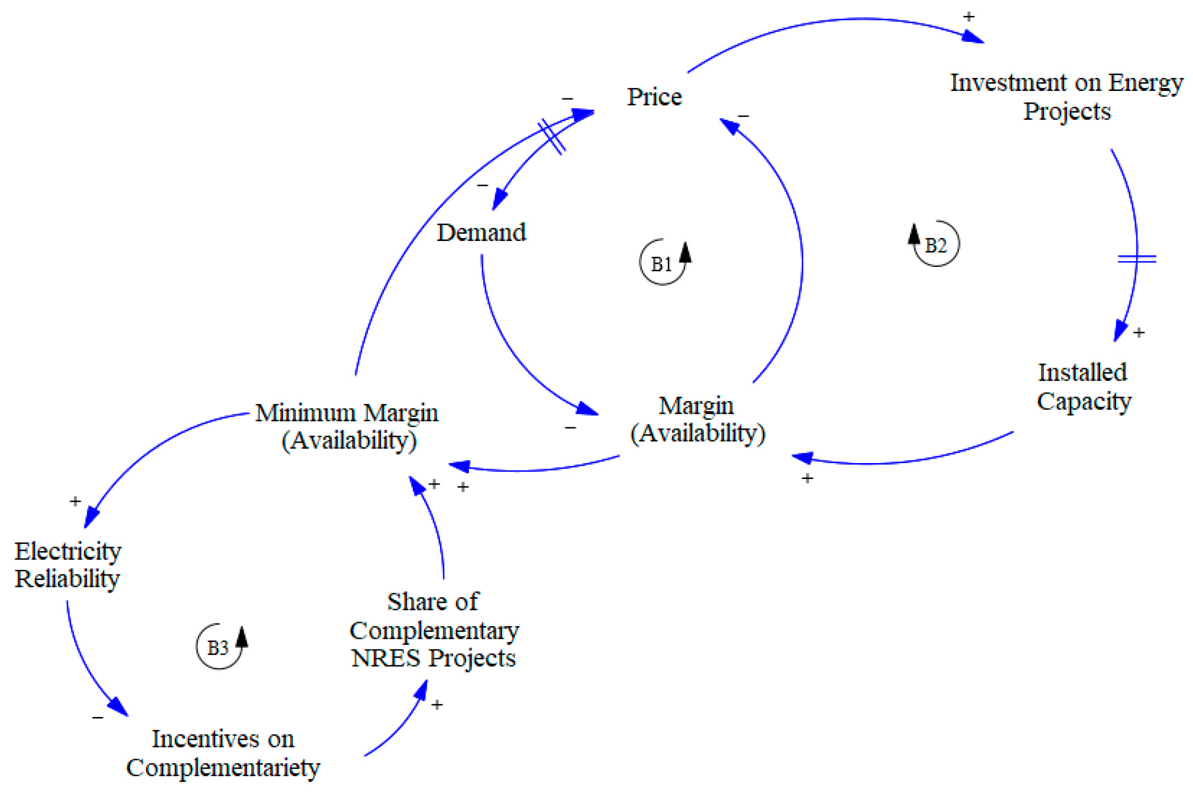
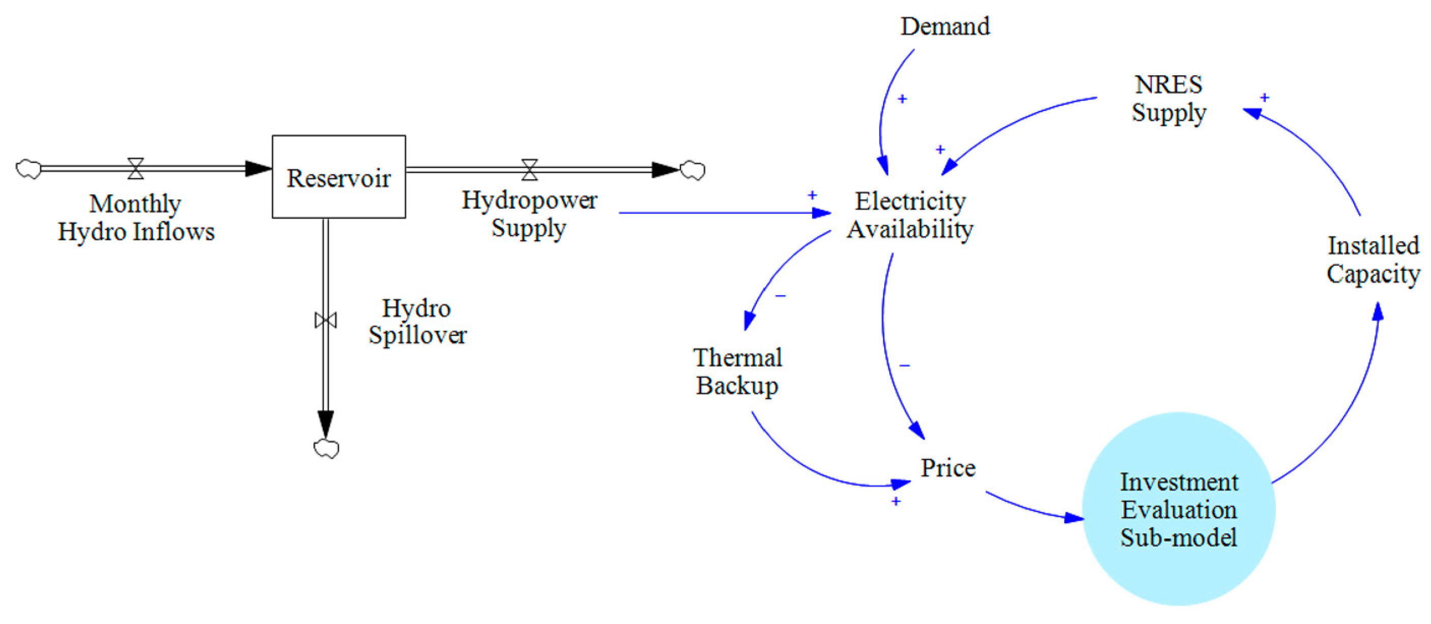
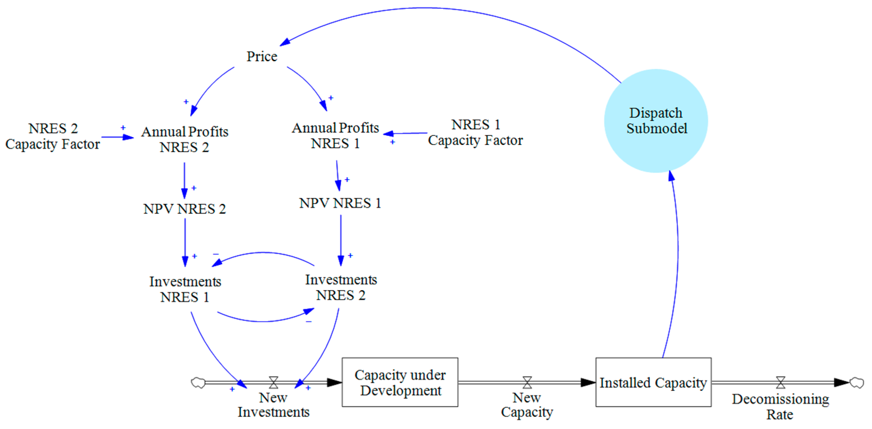
4.1. Model Description

This study employs a system dynamics approach, implemented in Vensim software (https://vensim.com/), to model the Colombian electricity system over a 20-year horizon. Input data for renewable energy availability and hydropower inflows were derived from XM, Colombia’s electricity system operator. Demand projections were based on national electricity consumption forecasts. The complete model equations are included in Appendix A.

Figure 1 provides a visual representation for the dynamics of the electricity system when incentives to complementarity are incorporated.

In this diagram, two feedback loops observed in any market can be identified:

• Balancing Loop B1 (Price–Demand Response): Increased demand reduces the availability margin, raising electricity prices and prompting demand reduction.
• Balancing Loop B2 (Investment–Price Dynamics): Higher prices incentivize new investments in generation capacity, increasing availability and stabilizing prices.

Given that new capacity will primarily come from NRES, a third feedback loop is introduced to the diagram (B3), as intermittency must now be considered in electricity system simulations. To address this, the model introduces the concept of a minimum availability margin, representing the lowest level of renewable electricity available at any time, accounting for climatic variability. When this margin approaches zero, the system relies on thermal plants to meet demand, risking shortages, price spikes, or rationing.

Although additional NRES capacity increases average system availability, it may not improve the minimum margin if the new capacity does not generate electricity during low-availability periods. For instance, solar projects cannot improve nighttime availability, even if they enhance overall output. However, profitability assessments typically prioritize total generation rather than addressing critical periods of low availability. This biases investments toward high-capacity-factor technologies, leaving projects that could stabilize the minimum margin underfunded.

To rectify this, government incentives could encourage investments in NRES projects that improve minimum availability. Such incentives would ensure critical support during low-availability periods, reducing reliance on thermal plants and stabilizing electricity prices. The balancing loop B3 demonstrates how incentives for complementary sources can enhance reliability by increasing the minimum margin while lowering costs through reduced thermal backup needs.

4.2. Complementarity Metric

Depending on the chosen metric to assess complementarity, a particular generation profile can be assigned a “higher” or “lower” complementarity value, as each metric is based on different parameters and quantifies distinct characteristics of the sources.

For this study, the Pearson correlation (r) was chosen as the metric for modelling incentives to complementarity, as it is the most commonly used metric in the literature.

Pearson correlation is a metric that directly quantifies how variables are linearly related [1]. Values close to −1 indicate high complementarity, whereas values close to 1 indicate low complementarity.

Traditionally, complementarity metrics are applied to assess the complementarity between the generation of two or more electricity sources. In this study, however, we use them to evaluate the complementarity of electricity sources with the overall system’s availability. Rather than measuring how two sources balance each other’s intermittent generation, we assess how well a specific source supports the overall balance of the electricity system.

This approach is driven by the idea that reliable systems should focus on reducing variability in overall electricity availability, rather than simply balancing generation between sources. A source may effectively complement another source’s generation deficit, but if the system already has sufficient electricity to meet demand during that time, additional generation—even if complementary—is unnecessary.

In the proposed model, Pearson correlation is measured for different sources with regards to the electricity availability margin of the system. These values are then used to determine the incentives offered to each source and how these incentives influence investment decisions.

4.3. Model Assumptions

To clearly identify the impact of complementarity on system behavior, we adjusted the model to restrict new investments to only two generation profiles. NRES1 represented very low complementarity (r = 1) with the system’s renewable electricity availability, while NRES2 represented very high complementarity (r = −1).

These two profiles were estimated from the renewable electricity availability margin at the beginning of the simulation (Figure 2).

From the availability margin curve, two normalized curves were plotted, which represented the generation profiles of NRES1 and NRES2 (Figure 3). NRES1 followed the exact shape of the availability curve; NRES2 was a mirror of the availability curve. This ensured that NRES1 obtained a correlation equal to 1, and NRES2 a correlation equal to −1.

The mathematical details of the model are presented below, starting with the Dispatch Sub-model in Section 4.3.1, and then the Investment Sub-model in Section 4.3.2.

4.3.1. Dispatch Sub-Model

The dispatch sub-model represents the monthly electricity dispatch, based on the following assumptions:

• Dispatch order: priority is given to NRES, followed by hydropower, and lastly, thermal plants if required.
• Electricity pricing: prices depend on the generation source, with NRES being the cheapest and thermal the most expensive.
• Thermal backup: thermal capacity is assumed to be sufficient to cover deficits.

Figure 4 illustrates a simplified representation of the dispatch sub-model.

The model determines the need for thermal generation based on electricity availability from renewable sources (NRES + Hydro). The resulting energy mix in the dispatch defines the electricity price at a given time. These prices are then fed into the investment sub-model, influencing investment decisions. Below are the equations used to calculate the availability of each source.

NRES Availability

This equation calculates the total availability of NRES in month j.

$${NRES Availability}_j=\sum _{i=1}^2{LF}_{i,j}\ast {IC}_i$$

(1)

where,

i = type of NRES;

j = month of the year;

${LF}_{i,j}$ = proportion of installed capacity effectively used to generate electricity, accounting for variability in resource availability (e.g., wind speeds, solar radiation); and

${IC}_i$ = the total capacity installed for source i, representing the maximum potential generation under optimal conditions.

Renewable Energy Availability (REA)

REA represents the balance between renewable energy supply and electricity demand for month j. It is calculated as:

$${\mathrm{R}\mathrm{E}\mathrm{A}}_{\mathrm{j}}={NRES \mathrm{A}\mathrm{v}\mathrm{a}\mathrm{i}\mathrm{l}\mathrm{a}\mathrm{b}\mathrm{i}\mathrm{l}\mathrm{i}\mathrm{t}\mathrm{y}}_{\mathrm{j}}+{Hydro Availability}_j-{Demand}_{\mathrm{j}}$$

(2)

If ${REA}_j$ is positive, it indicates a surplus of renewable energy (NRES and hydro combined). If it is negative, there is an energy shortfall that needs to be compensated by other sources, such as thermal generation.

Thermal Generation Requirement

This equation calculates the thermal energy generation required to balance the grid, depending on the value of REA:

$${Generation}_{\mathrm{T}\mathrm{h}\mathrm{e}\mathrm{r}\mathrm{m}\mathrm{a}\mathrm{l},\mathrm{j}}=\mathrm{M}\mathrm{a}\mathrm{x}(-{\mathrm{R}\mathrm{E}\mathrm{A}}_{\mathrm{j}},0)$$

(3)

If ${REA}_j\ge 0$, this implies a renewable energy surplus. In this case, no thermal generation is needed. If ${REA}_j<0$, it indicates a shortfall in renewable energy, and thermal generation steps in to meet the deficit. This ensures thermal generation is only used when necessary to meet demand, minimizing its operation in scenarios with sufficient renewable energy.

4.3.2. Investment Sub-Model

Figure 5 illustrates a simplified representation of the investment evaluation sub-model.

To assess the economic viability of NRES, the model calculates the revenue, profit, and net present value (NPV) per megawatt (MW) of installed capacity for each type of source. These calculations account for the variability in resource availability, operational costs, and financial incentives for complementarity. The following equations outline the methodology:

Monthly Revenues per MW

$${\mathrm{R}\mathrm{e}\mathrm{v}\mathrm{e}\mathrm{n}\mathrm{u}\mathrm{e}/\mathrm{M}\mathrm{W}}_{\mathrm{i},\mathrm{j}}={\mathrm{L}\mathrm{F}}_{\mathrm{i},\mathrm{j}}\ast {\mathrm{P}}_{\mathrm{j}}$$

(4)

where $P_j$ represents the electricity price during month j, reflecting seasonal and demand-driven variations.

This equation quantifies the revenue potential of each energy source based on its capacity utilization and market conditions.

Annual Profit per MW

$${\mathrm{A}\mathrm{n}\mathrm{n}\mathrm{u}\mathrm{a}\mathrm{l} \mathrm{P}\mathrm{r}\mathrm{o}\mathrm{f}\mathrm{i}\mathrm{t}/\mathrm{M}\mathrm{W}}_{\mathrm{i}}=\sum _{\mathrm{j}=1}^{12}{\mathrm{R}\mathrm{e}\mathrm{v}\mathrm{e}\mathrm{n}\mathrm{u}\mathrm{e}/\mathrm{M}\mathrm{W}}_{\mathrm{i},\mathrm{j}}-{\mathrm{M}\mathrm{o}\mathrm{n}\mathrm{t}\mathrm{h}\mathrm{l}\mathrm{y} \mathrm{O}\mathrm{P}\mathrm{E}\mathrm{X}}_{\mathrm{i},\mathrm{j}}$$

(5)

The annual profit per megawatt of installed capacity is obtained by summing the monthly revenues across the 12 months of the year and subtracting the corresponding monthly operational costs (${Monthly OPEX}_{i,j}$) incurred as a result of maintaining and operating the energy source in month j.

This calculation determines the net financial performance of each source over a year after accounting for operational expenditures.

NPV per MW

$${\mathrm{N}\mathrm{P}\mathrm{V}/\mathrm{M}\mathrm{W}}_{\mathrm{i}}=\sum _{\mathrm{t}=0}^{\mathrm{n}}{\displaystyle \frac{{\mathrm{A}\mathrm{n}\mathrm{n}\mathrm{u}\mathrm{a}\mathrm{l} \mathrm{P}\mathrm{r}\mathrm{o}\mathrm{f}\mathrm{i}\mathrm{t}/\mathrm{M}\mathrm{W}}_{\mathrm{i},\mathrm{t}}}{{(1+\mathrm{k})}^{\mathrm{t}}}}-{\mathrm{I}\mathrm{I}}_{\mathrm{i}}\ast (1-{\mathrm{C}\mathrm{D}}_{\mathrm{i}})$$

(6)

The NPV per MW reflects the long-term profitability of an energy source by evaluating its annual profits over the project lifespan (n), discounted by a factor k. The calculation incorporates:

${II}_i=$ the capital required to install one MW of capacity for energy source I; and

${CD}_{\mathit{i}}=$ the complementarity discount on initial investments, applied to projects in proportion to their correlation with the system’s electricity availability.

5. Results

To analyze the effects of incentivizing complementarity between energy sources and the system’s electricity availability margin, we propose four scenarios that help illustrate the system’s behavior with and without incentives. This will provide the basis for comparisons of potential benefits and tradeoffs from leveraging the complementarity nature of NRES in the system. The first two scenarios analyze the system without incentives, and the last two scenarios analyze the system when incentives are incorporated.

The renewable electricity availability margin (REAM) is the main variable used in this model to analyze the evolution of the system’s reliability. This margin is defined by Equation (7):

$${\mathrm{R}\mathrm{E}\mathrm{A}\mathrm{M}}_{\mathrm{j}}={\displaystyle \frac{{\mathrm{R}\mathrm{E}\mathrm{A}}_{\mathrm{j}}}{{\mathrm{D}\mathrm{e}\mathrm{m}\mathrm{a}\mathrm{n}\mathrm{d}}_{\mathrm{j}}}}$$

(7)

Values higher than 0 indicate that supply from NRES and hydropower is enough to fulfill the demand. Values lower than 0 mean that the supply is not sufficient to satisfy the demand, and thermal generation is required.

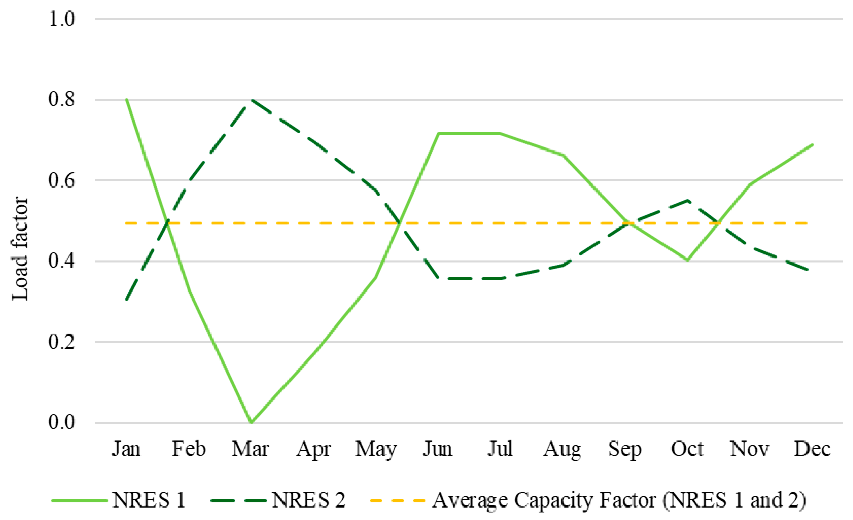
5.1. Scenario 1: Same Annual Generation (SAG)

This scenario serves as a baseline for understanding how a free electricity market, without complementarity incentives, prioritizes investments when NRES have identical annual generation outputs. This simplified situation aims to illustrate the natural behavior of the market in optimizing investments based purely on capacity factors and electricity prices, without the influence of variability or complementarity concerns.

In the SAG scenario, NRES1 and NRES2 are assumed to have the same annual capacity factor of 0.5. This ensures that both sources generate equal amounts of electricity over a year, regardless of their monthly variations. The market’s behavior is then evaluated based on how these variations affect profitability and system reliability.

Figure 6 shows the generation profiles of NRES1 and NRES2. Despite their differences in monthly output, the equal annual generation ensures that profitability depends primarily on electricity prices during the periods of production. This creates a level playing field where the market can naturally allocate investments based on the timing of generation relative to demand.

Figure 7 illustrates the REAM over time for this scenario. The results indicate that the market is capable of achieving a balance between supply and demand without relying on thermal backup. Over time, investments are directed toward sources that generate electricity during high-demand periods, thereby reducing variability in the availability margin. Importantly, no shortages occur, and variability decreases significantly compared to the initial conditions.

This outcome demonstrates that under idealized conditions—where NRES projects have the same annual output—the market inherently prioritizes investments that align with system needs. This negates the necessity for complementarity incentives, as electricity prices alone act as a sufficient signal to drive optimal investment decisions.

While this scenario highlights the efficiency of market-driven optimization under simplified conditions, it does not account for the real-world variability of NRES capacity factors. In practical settings, renewable energy sources often exhibit significant differences in annual generation due to geographic and climatic factors. These differences can disrupt the natural allocation of investments, leading to inefficiencies and system vulnerabilities. This is particularly relevant in the Colombian context, where solar and wind resources are geographically concentrated and subject to weather-dependent variability.

The results from this scenario underscore the importance of addressing variability in real-world electricity markets. While the market can optimize investments under equal generation conditions, the following scenarios demonstrate the need for targeted incentives to account for variability and ensure a balanced, reliable energy mix.

The SAG scenario establishes a theoretical benchmark for understanding how complementarity incentives interact with market dynamics. The next scenario (DAG) introduces variability in annual generation outputs, revealing the challenges that arise when market forces alone are insufficient to achieve optimal outcomes.

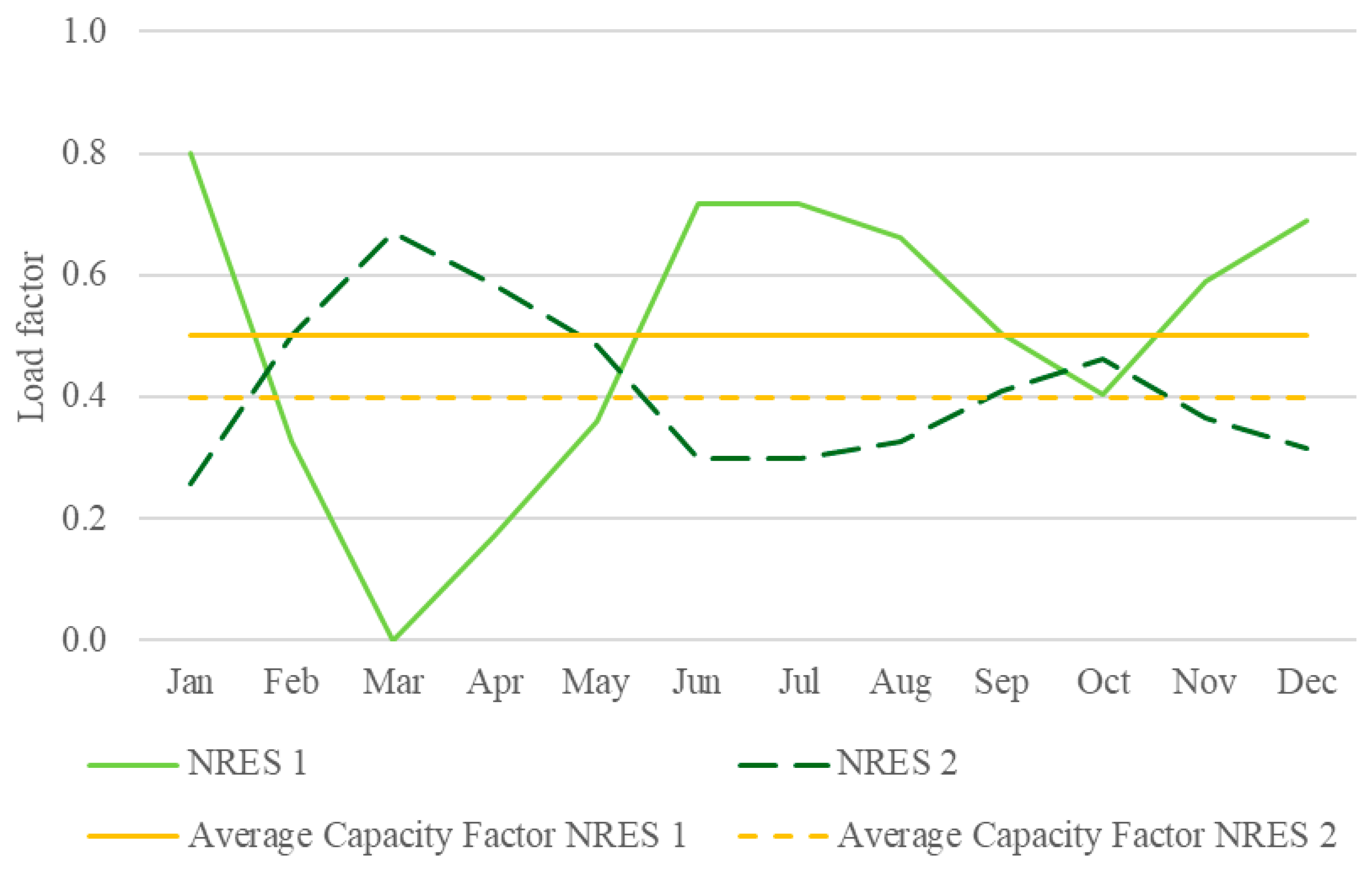
5.2. Scenario 2: Different Annual Generation (DAG)

Building on the baseline established in the SAG scenario, this scenario introduces a more realistic condition where NRES projects exhibit differences in annual generation outputs. Specifically, the annual generation of NRES2 is reduced by 10%, while NRES1 retains its original capacity factor, as observed in Figure 8. This scenario explores how variability in generation impacts investment decisions and overall system performance in the absence of complementarity incentives.

Despite NRES2 offering a complementary generation profile that aligns better with periods of low availability, its lower annual generation reduces its profitability relative to NRES1. As shown in Figure 9, this results in a significant skew in investments, with 70% of total capacity directed toward NRES1 by the end of the simulation.

This imbalance highlights a critical limitation of market-driven decision-making: profitability metrics, such as capacity factor and revenue potential, often outweigh system-level considerations like reliability and complementarity. Consequently, while overall renewable capacity increases, it fails to address critical periods of low availability.

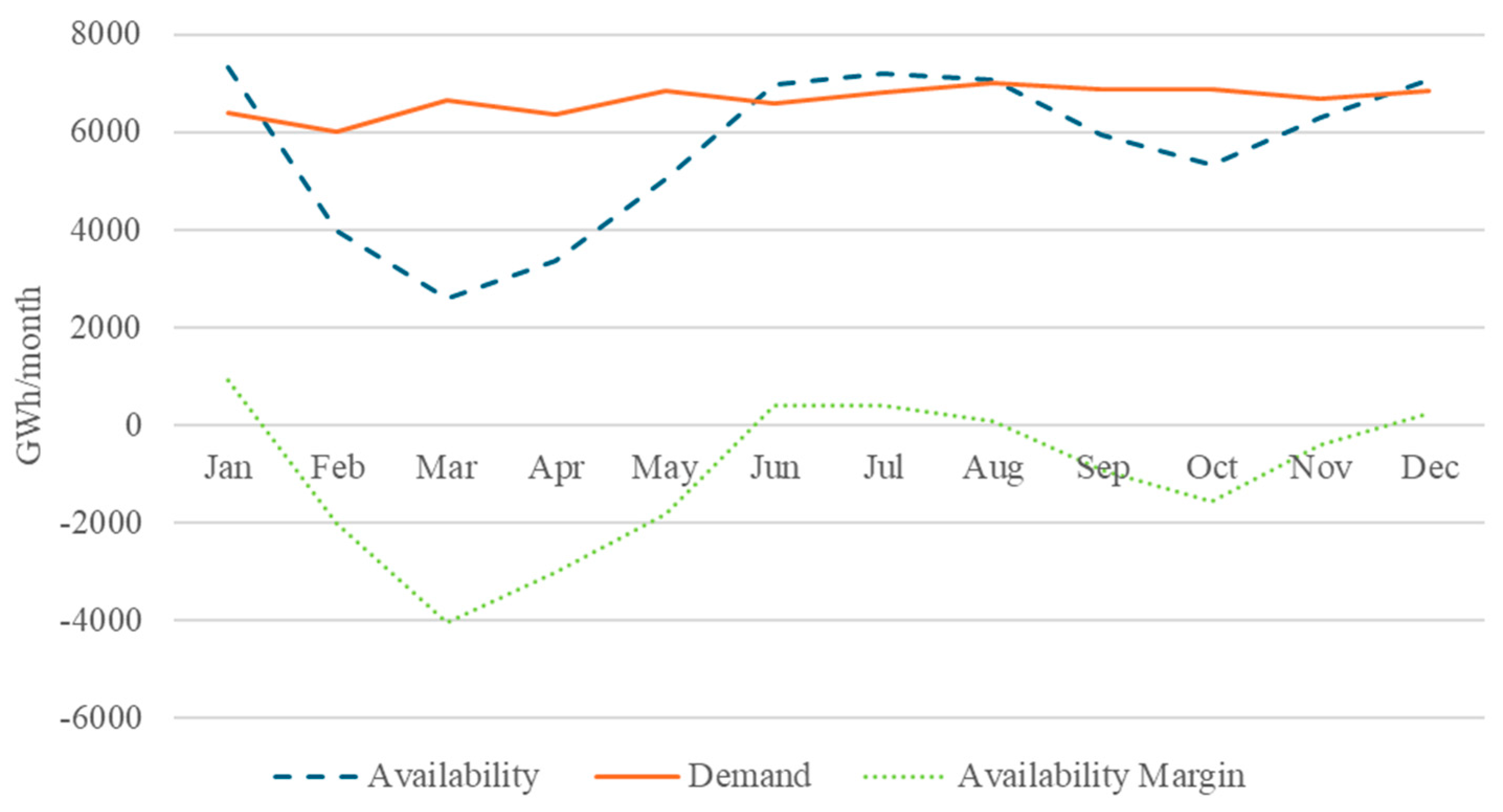
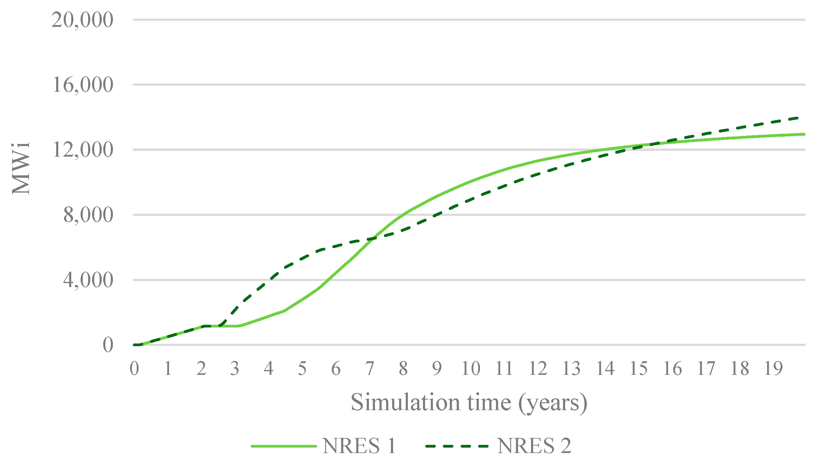
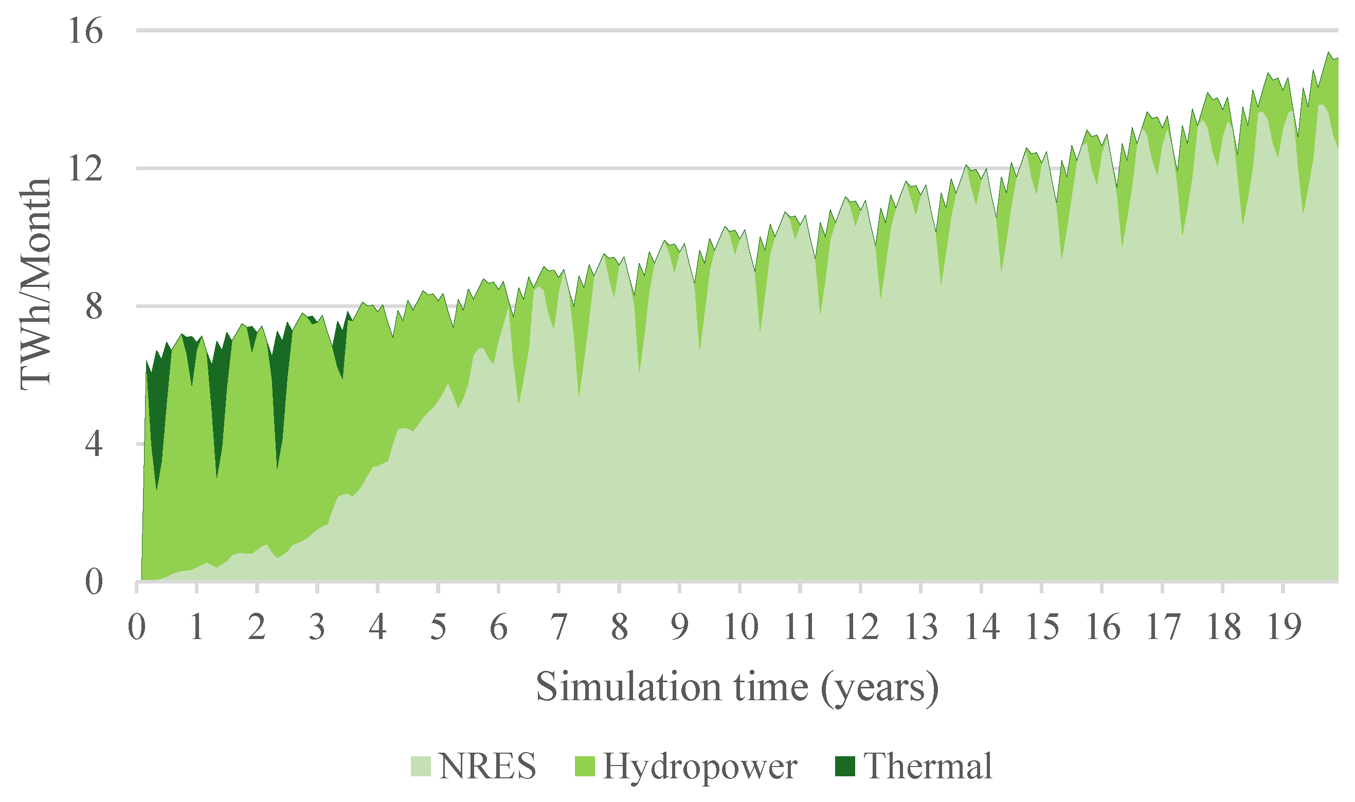
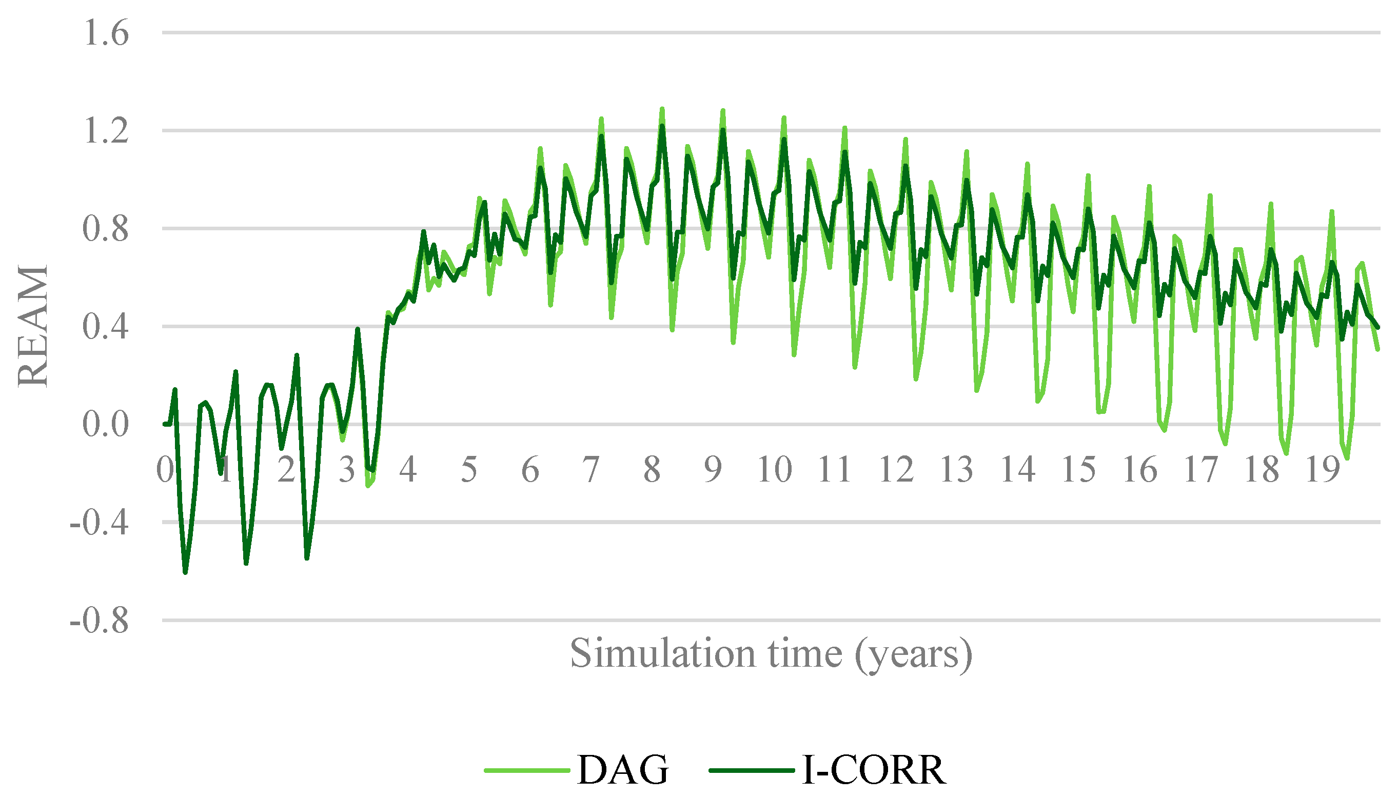
5.2.1. Security of Supply

Figure 10 illustrates REAM over the simulation period. While the system initially benefits from increased renewable capacity, the bias toward NRES1 exacerbates variability in electricity availability.

Peaks in availability increase disproportionately compared to minimum levels, resulting in significant fluctuations. By the end of the simulation, the system still relies on thermal backup during low-availability periods, undermining reliability and increasing costs.

Figure 11 further underscores this inefficiency, showing that NRES1 generates electricity primarily during periods when demand is already met, while shortages persist during other times. This mismatch leads to higher reliance on costly thermal generation, particularly in the early years of the simulation.

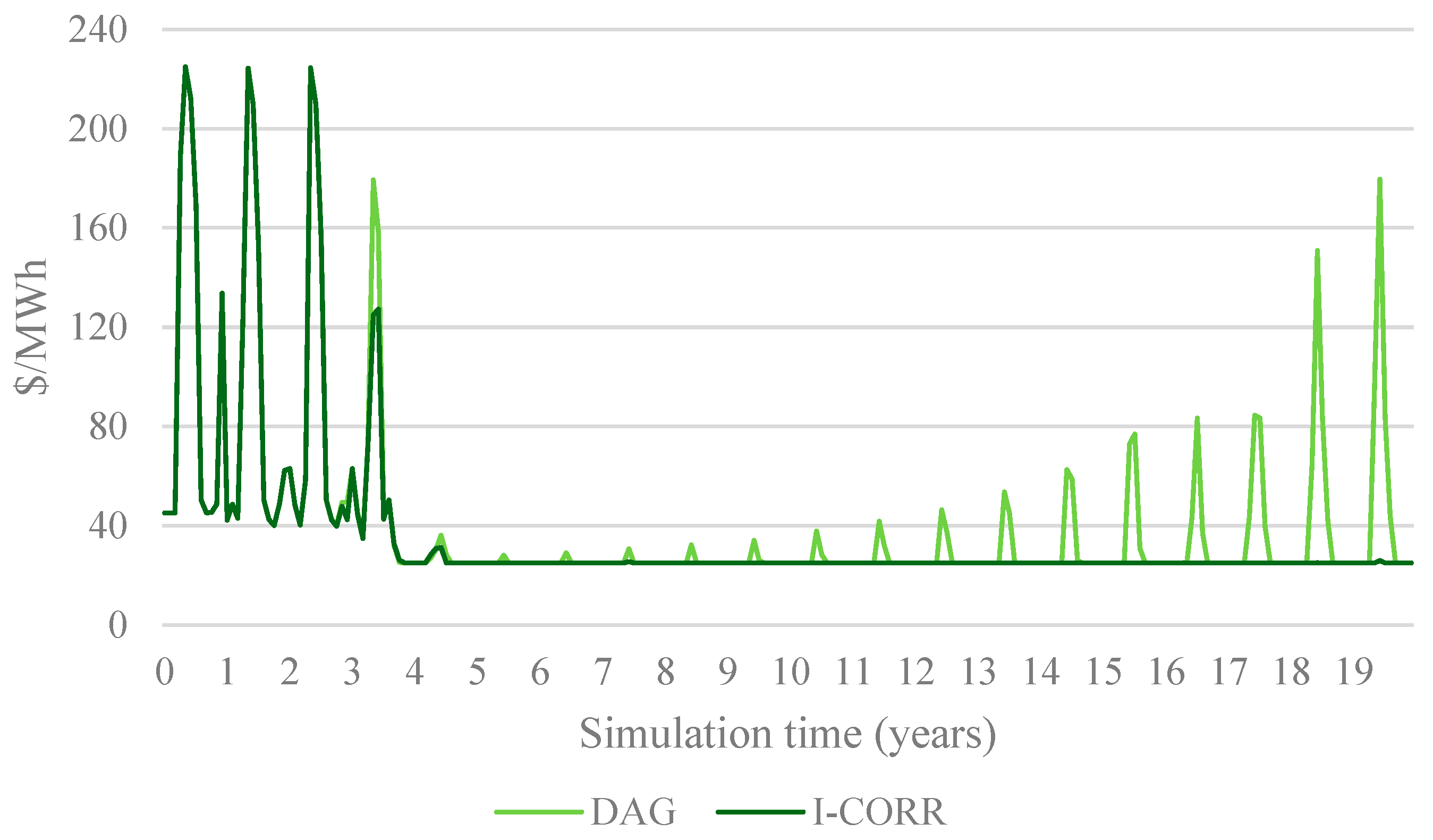
5.2.2. Affordability

From an affordability perspective, the overreliance on NRES1 drives inefficiencies that increase system costs. As shown in Figure 12, electricity prices initially decline due to increased capacity but rise again when capacity fails to meet growing demand, particularly during low-availability periods. This volatility underscores the limitations of relying solely on market forces to optimize investments in renewable energy.

The DAG scenario demonstrates that market-driven investment decisions, based on profitability alone, are insufficient to optimize the energy mix in systems with variable renewable resources. While NRES2’s complementary generation profile offers clear reliability benefits, its reduced annual output makes it less attractive to investors, leaving the system vulnerable to periods of low availability.

This scenario also highlights the trade-offs inherent in current evaluation metrics, such as the Levelized Cost of Energy (LCOE), which prioritize total generation over system stability. Without targeted incentives, the system fails to achieve a balance between reliability, affordability, and sustainability.

The challenges observed in this scenario underscore the need for policy interventions to guide investments toward complementary sources. The next scenario (I-CORR) examines how incentivizing complementarity can address these challenges, enhancing system reliability and reducing reliance on thermal generation.

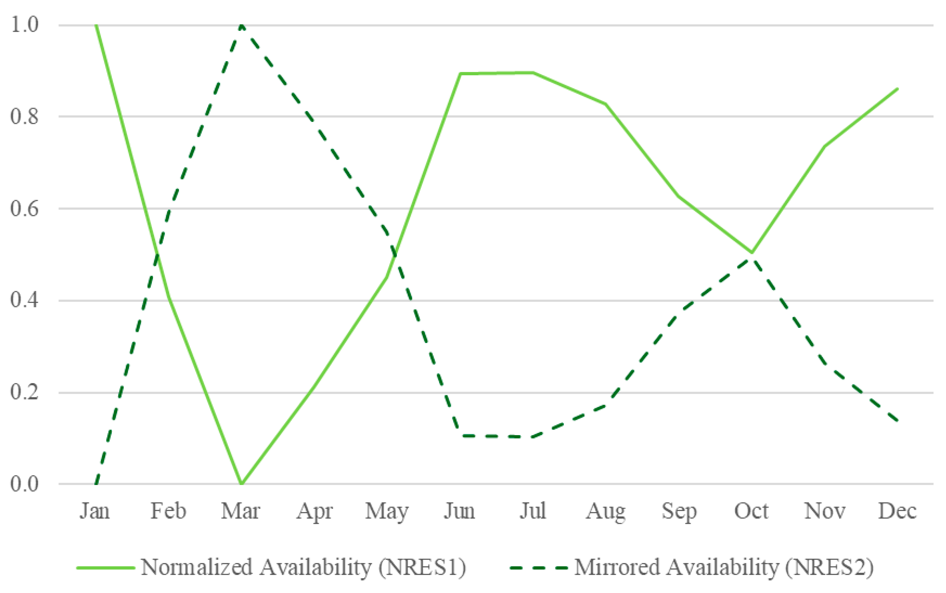
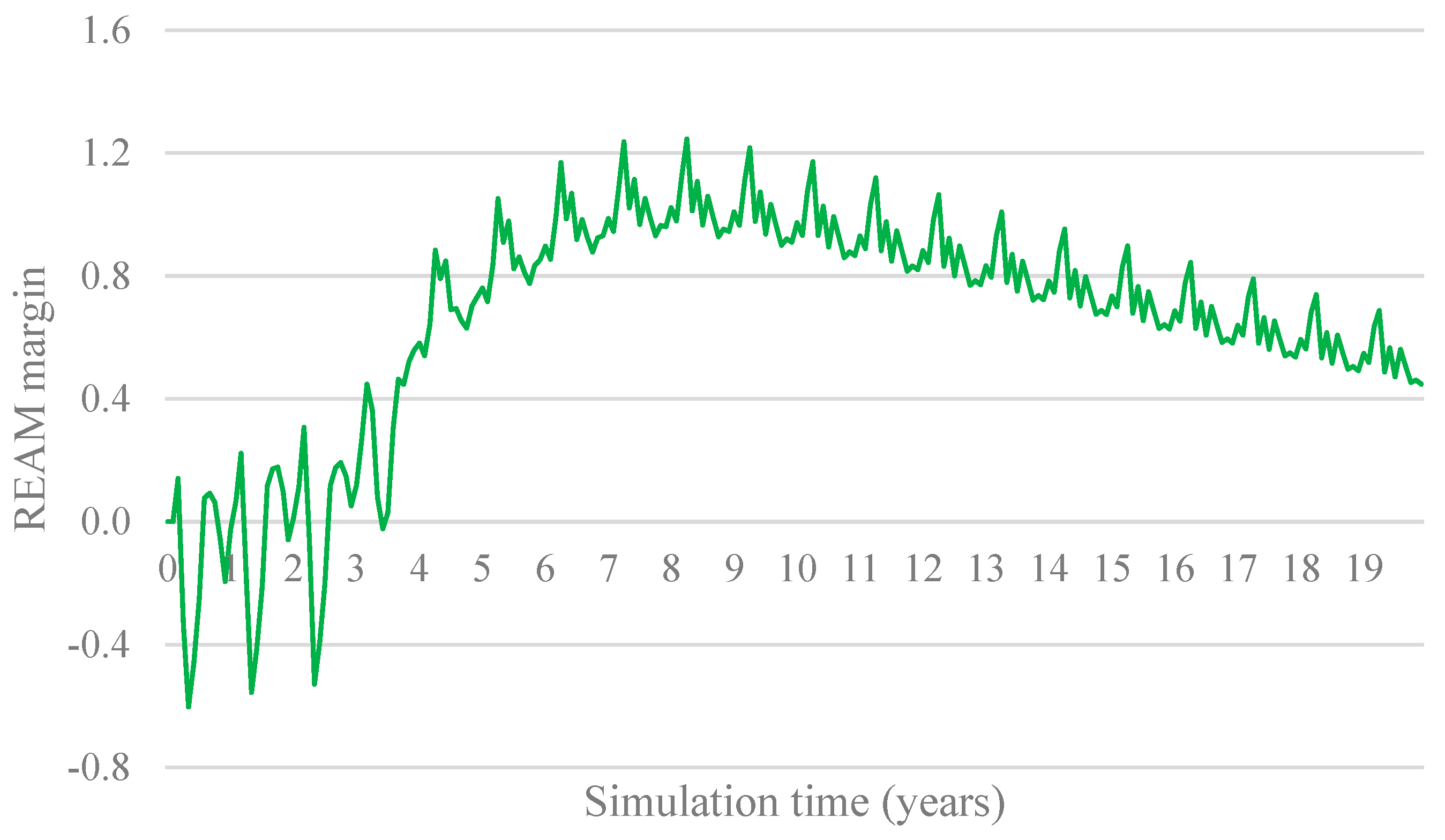
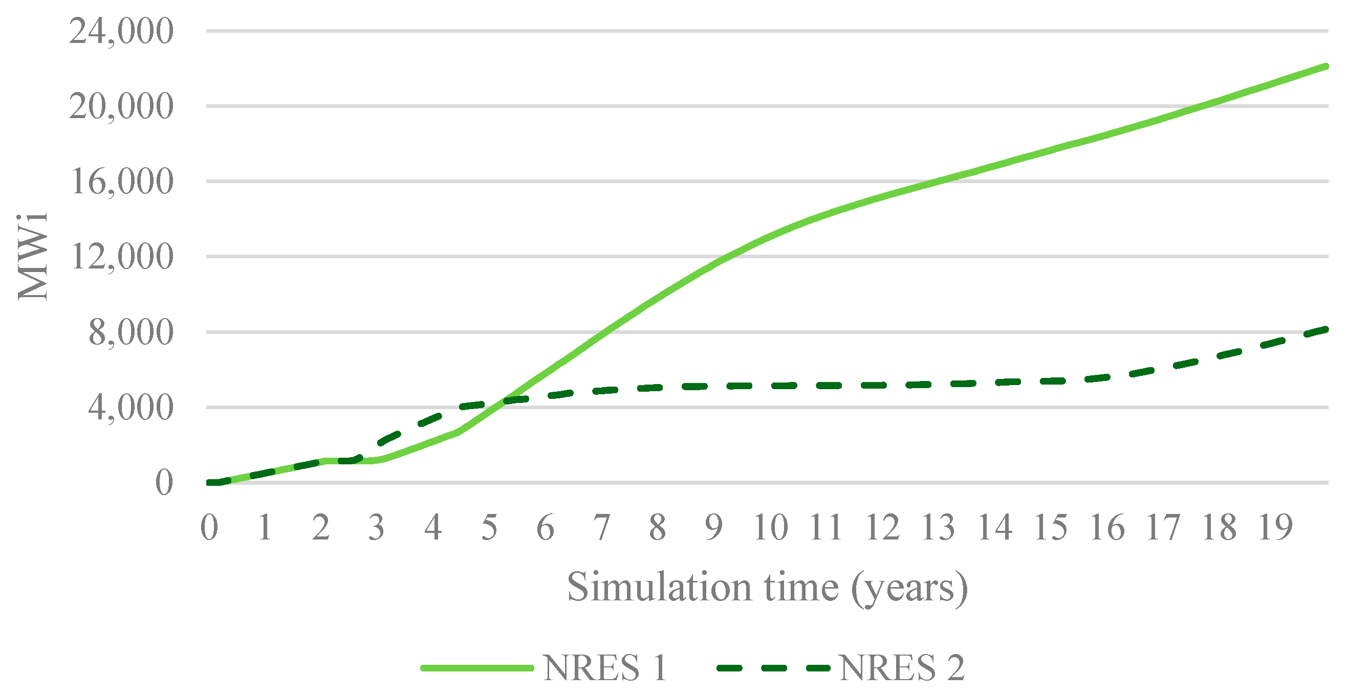
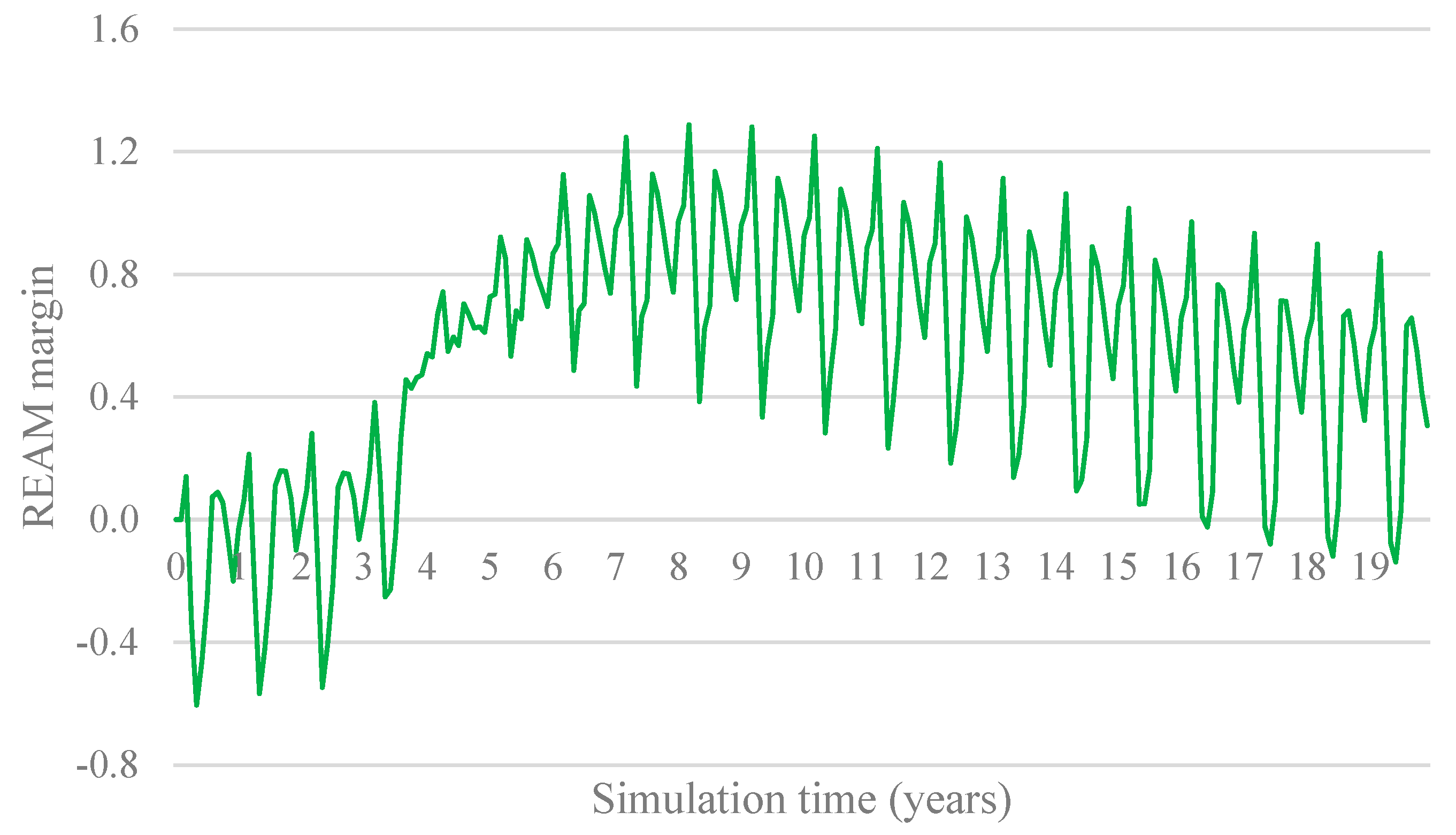
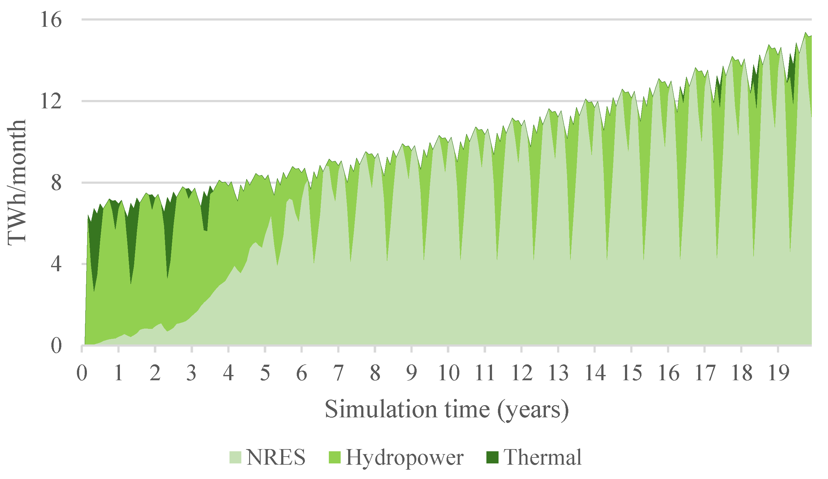
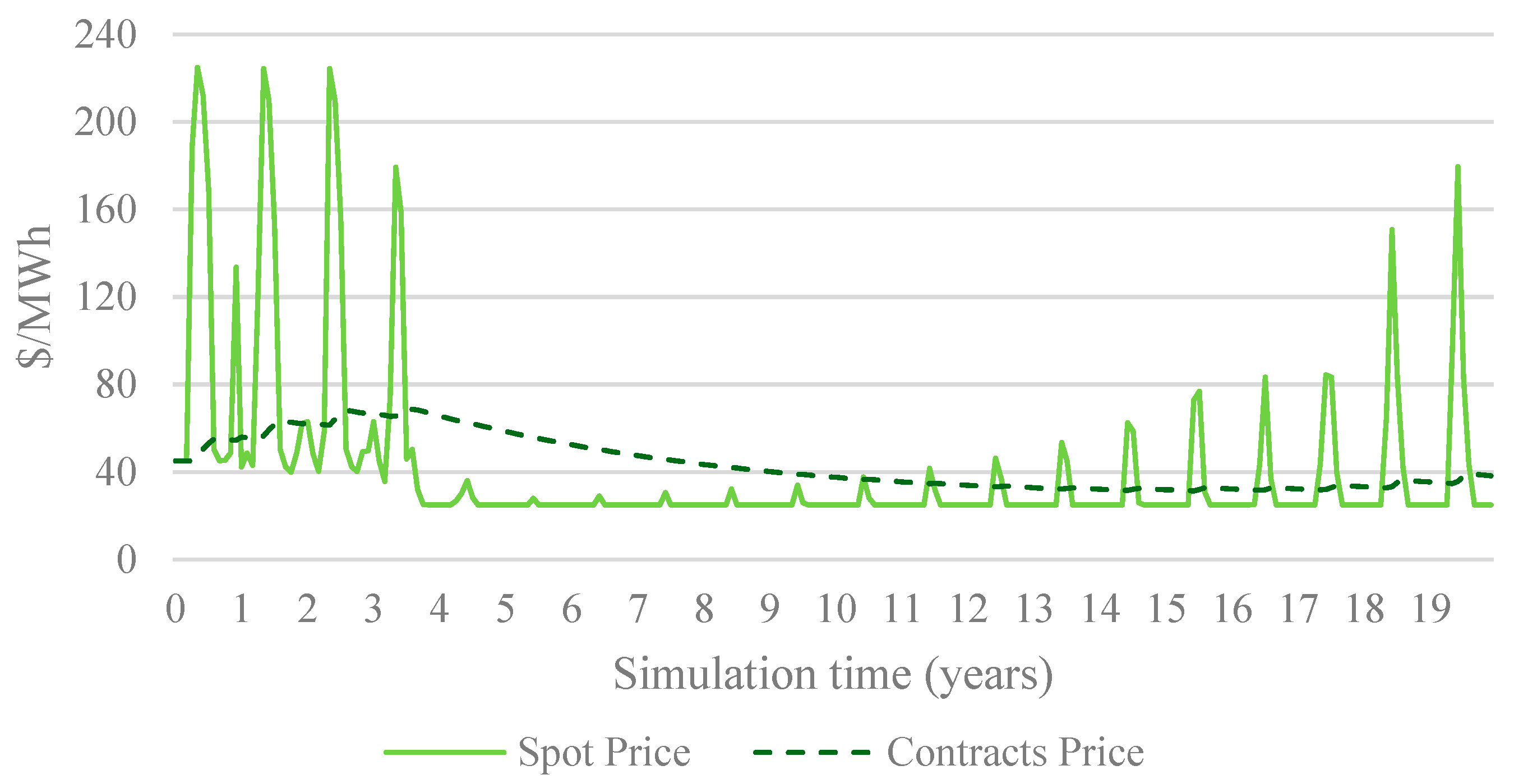
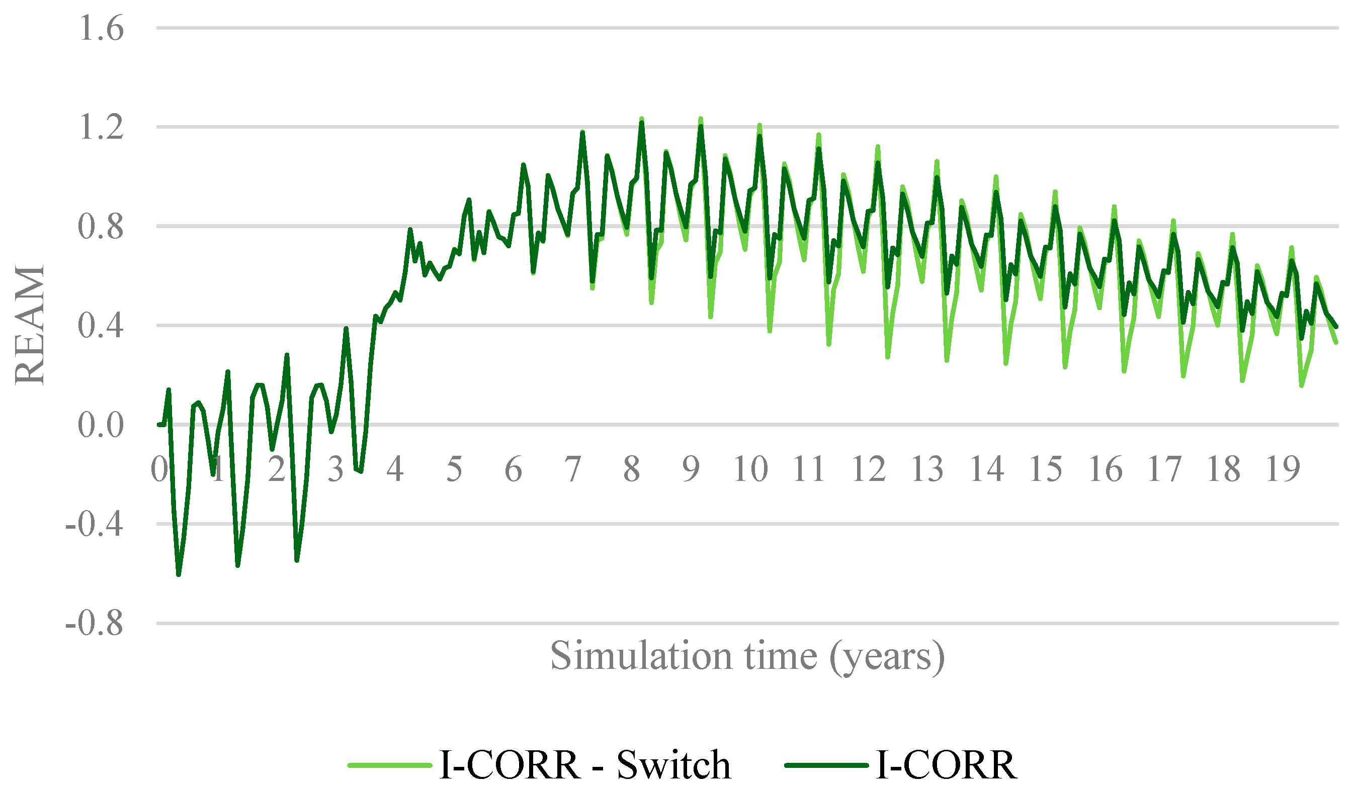
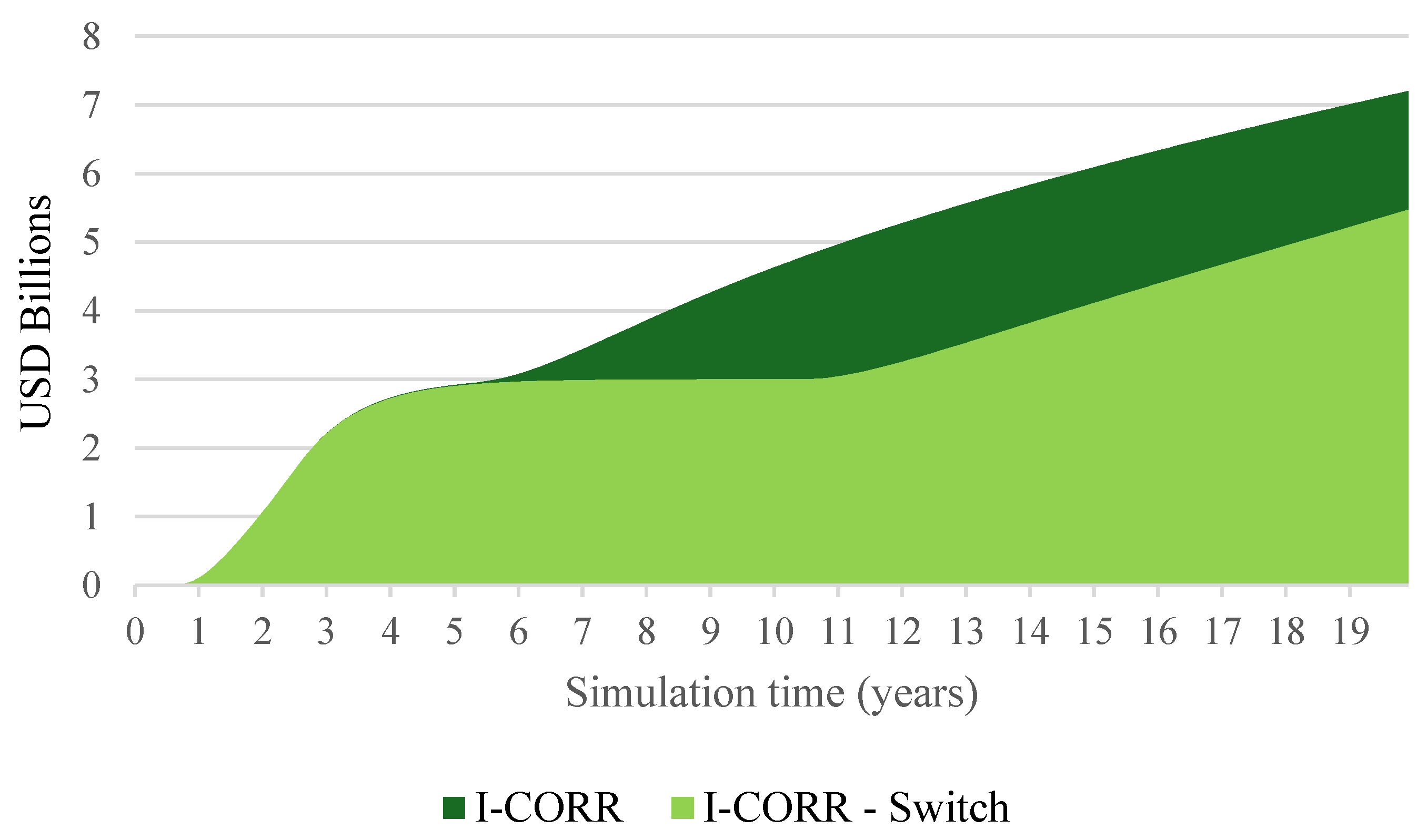
5.3. Scenario 3: Incentivizing Complementarity (I-CORR)

This scenario explores the impact of implementing complementarity-based incentives on the electricity mix and system performance. By offering capital cost discounts proportional to the complementarity of a NRES with the overall system availability, this approach aims to correct the market imbalances observed in the DAG scenario. The Pearson correlation coefficient serves as the primary metric to evaluate complementarity, with higher discounts allocated to sources that exhibit stronger negative correlations with the availability margin.

5.3.1. Security of Supply

Figure 13 demonstrates the changes in installed capacity for both NRES1 and NRES2 when complementarity incentives are applied. Unlike the DAG scenario, investments are more evenly distributed between the two sources, with NRES2 capturing a larger share despite its lower annual generation. This shift is driven by the financial attractiveness of the incentives, which partially offset NRES2’s reduced profitability.

By encouraging investments in complementary sources, the system achieves a more balanced energy mix that aligns generation patterns with periods of low availability. This outcome highlights the effectiveness of complementarity incentives in addressing the market inefficiencies observed in the previous scenario.

The effects of incentivizing complementarity on system reliability are evident in Figure 14, which shows monthly electricity generation by source. Early in the simulation, the system relies heavily on hydropower and thermal generation to meet demand. However, as investments in NRES2 increase, hydropower begins to serve as a flexible backup, and the reliance on thermal generation is eliminated entirely by the middle of the simulation period.

Figure 15 illustrates the Renewable Electricity Availability Margin (REAM) over time. Unlike the DAG scenario, the availability margin remains consistently positive, indicating that the system meets demand throughout the simulation without the need for thermal backup. Additionally, the variability of the availability margin is significantly reduced, enhancing system stability and minimizing the risks of electricity shortages or price volatility.

5.3.2. Affordability

From an affordability perspective, complementarity incentives reduce electricity prices by optimizing the energy mix and minimizing reliance on expensive thermal generation. Figure 16 compares electricity spot prices for the DAG and I-CORR scenarios. The results show a notable decrease in price volatility under I-CORR, as the system avoids peak price spikes associated with thermal generation. Contract prices also stabilize, delivering long-term cost savings to consumers.

5.3.3. Limitations of the Metric

While the I-CORR scenario demonstrates the benefits of incentivizing complementarity, it also highlights some limitations of using Pearson correlation as a complementarity metric. This coefficient only measures the similarity between the availability curve and the generation profile, ignoring the magnitude of the availability margin.

This can lead to two undesirable effects:

• Incentives may continue to drive investments even when electricity availability is already sufficient.
• Complementary investments may be deprioritized during periods of low availability if the correlation coefficient decreases.

To address these limitations, an additional threshold for minimum availability could be introduced. By activating incentives only when the availability margin falls below a specified level, this refinement would ensure that investments are directed toward projects that provide the greatest reliability benefits.

Figure 17 shows the effects on the availability margin when a threshold of 0.2 is introduced to the I-CORR scenario. This means that incentives will be activated only when the REAM falls below 0.2. As seen in the graph, the variation in the margin is higher, as the switch lowers the incentives to complementary sources, and therefore, the investments flowing to this source. However, the graph shows that the demand is still supplied at all times, as the margin is always above 0. The results suggest that the switch effectively minimizes unnecessary incentives while maintaining system reliability.

In the final years of simulation, the REAM falls below the threshold (0.2), which causes incentives to be turned on again. This will increase investments in the following years, preventing the REAM from falling below 0.

As shown in Figure 18, incorporating this threshold reduces the cumulative cost of incentives by up to 24%, further enhancing the cost-effectiveness of the approach.

The I-CORR scenario underscores the transformative potential of complementarity incentives in achieving a reliable, affordable, and sustainable electricity system. By addressing the weaknesses of market-driven investment dynamics, these incentives create a more balanced energy mix that reduces variability, eliminates reliance on thermal generation, and stabilizes electricity prices.

The findings from this scenario provide a compelling case for implementing complementarity-based incentives in renewable energy markets. However, additional refinements to the complementarity metric, as well as further analysis of systems with limited storage capacity, are necessary to maximize the benefits of this approach. The next section explores these considerations in greater detail.

6. Discussion

This study highlights the transformative potential of incentivizing complementarity between renewable energy sources (NRES) and electricity system availability. By addressing the challenges of intermittency and variability, complementarity-based incentives offer a pathway to achieve a reliable, affordable, and sustainable energy transition. This section synthesizes the key findings, explores their broader implications, and identifies areas for future research.

6.1. The Role of Hydro Storage in Colombia’s Electricity System

In the Colombian context, the integration of NRES into a hydropower-dominated system demonstrates how complementarity incentives can optimize resource utilization. Hydropower’s inherent flexibility serves as a backup during periods of variability, while complementarity-driven investments stabilize the minimum availability margin. This dynamic reduces emissions and fossil fuel reliance, advancing Colombia’s renewable energy targets.

6.2. Leveraging Colombia’s Renewable Resources for Complementarity

Colombia’s geographical advantages—including abundant solar, wind, and hydro resources—position it as a leader in renewable energy integration. However, the uneven distribution of NRES projects, concentrated primarily in the northern regions, creates challenges for grid reliability and transmission capacity. Complementarity incentives address this issue by encouraging geographically and temporally balanced investments. By leveraging the complementarity between solar, wind, and hydro resources, Colombia can reduce its reliance on thermal generation during periods of low hydrology or high demand.

Additionally, complementarity incentives align with Colombia’s energy transition goals by fostering a cleaner, more diversified electricity matrix. As demonstrated in this study, these incentives not only improve system reliability but also support the country’s broader climate commitments by reducing greenhouse gas emissions and enhancing energy affordability.

6.3. Broader Implications for Low-Storage Systems

While this study focuses on Colombia’s hydropower-rich electricity system, the findings also offer valuable insights for regions with limited storage capacity. Systems that lack large-scale energy storage often face heightened challenges related to renewable energy intermittency. In such contexts, complementarity incentives become even more critical for maintaining system reliability.

Without adequate storage, variability in NRES generation can lead to frequent electricity shortages, greater reliance on thermal backup, and increased price volatility. Complementarity incentives address these challenges by directing investments toward renewable projects that align with periods of low availability, stabilizing the minimum availability margin and ensuring consistent electricity supply. This approach reduces the risks associated with low generation during critical periods and helps mitigate the cost burden of integrating NRES into storage-limited grids.

These implications highlight the adaptability and scalability of complementarity incentives. Policymakers in regions with limited storage should prioritize such mechanisms to enhance reliability, affordability, and sustainability during the energy transition. By tailoring incentive structures to local system conditions, governments can effectively balance energy security and renewable integration goals.

6.4. Future Research Directions

Building on the findings of this study, future research should:

• Explore granular temporal scales: Investigate complementarity at finer temporal resolutions, such as daily or hourly scales, to better capture the short-term dynamics of renewable energy integration.
• Analyze real-world data: Apply the proposed framework to real-world datasets from diverse geographic regions to validate its applicability and refine the complementarity metrics.
• Incorporate storage technologies: Assess the interplay between complementarity incentives and emerging storage technologies, such as battery storage, to determine their combined impact on system reliability and affordability.
• Evaluate dynamic incentive structures: Develop adaptive policy frameworks that adjust incentives in real-time based on system conditions, further enhancing cost-effectiveness and reliability.

7. Conclusions

This study analyzed the potential of incentivizing complementarity between NRES and electricity system availability, highlighting benefits for reliability, affordability, and sustainability. A literature review identified a gap in research on complementarity incentives and their system-wide impacts. To address this, the study used system dynamics modeling to assess complementarity incentives and evaluate metrics, with Pearson correlation serving as the primary measure.

Pearson correlation was assessed as a tool to incentivize complementary NRES. This metric successfully encouraged investments in electricity sources that enhance system re-liability. A key limitation identified was its inability to account for the absolute value of electricity availability. This metric insufficiently emphasized ensuring minimum availability levels, which are critical for system stability. To maximize the benefits of complementarity incentives, Pearson correlation should incorporate an analysis of the minimum availability margin. Incentives should increase during periods of low availability and de-crease when availability is high, directing support to where complementary generation can most effectively bolster the system.

This study demonstrates that complementarity-based incentives can significantly enhance system reliability, reduce reliance on thermal generation, and support energy transitions. Refining complementarity metrics to account for minimum availability and applying these findings to real-world data are critical next steps. Exploring complementarity at more granular levels, such as daily or hourly variations, would further unlock flexibility and resilience, making this approach a powerful tool for guiding investments in renewable energy systems globally.

References

1. Jurasz, J.; Canales, F.A.; Kies, A.; Guezgouz, M.; Beluco, A. A review on the complementarity of renewable energy sources: Concept, metrics, application and future research directions. Sol. Energy 2020, 195, 703–724. [Google Scholar] [CrossRef]
2. Bekirsky, N.; Hoicka, C.; Brisbois, M.; Camargo, L.R. Many actors amongst multiple renewables: A systematic review of actor involvement in complementarity of renewable energy sources. Renew. Sustain. Energy Rev. 2022, 161, 112368. [Google Scholar] [CrossRef]
3. Hoicka, C.E.; Lowitzsch, J.; Brisbois, M.C.; Kumar, A.; Camargo, L.R. Implementing a just renewable energy transition: Policy advice for transposing the new European rules for renewable energy communities. Energy Policy 2021, 156, 112435. [Google Scholar] [CrossRef]
4. Gonzalez-Salazar, M.; Poganietz, W.R. Evaluating the complementarity of solar, wind and hydropower to mitigate the impact of El Niño Southern Oscillation in Latin America. Renew. Energy 2021, 174, 453–467. [Google Scholar] [CrossRef]
5. Sterman, J.D. Business Dynamics: Systems Thinking and Modeling for a Complex World; McGraw Hill Education: New York, NY, USA, 2000; p. 1008. [Google Scholar]
6. Parra, L.; Gómez, S.; Montoya, C.; Henao, F. Assessing the Complementarities of Colombia’s Renewable Power Plants. Front. Energy Res. 2020, 8, 575240. [Google Scholar] [CrossRef]
7. IDEAM. Atlas de Radiación Solar de Colombia. arXiv 2014, arXiv:1409.5722v1. [Google Scholar]
8. Peña, R.; Gallardo, P.; Castro, O. An Assessment Study of the Monthly Complementarity of Renewable Energy Resources in Colombia. 2018. Available online: https://www.researchgate.net/publication/326131594 (accessed on 1 July 2024).
9. IDEAM; UPME. Atlas de Viento y Energía Eólica de Colombia; IDEAM: Bogotá, Colombia, 2006. [Google Scholar]
10. Haley, B. Promoting low-carbon transitions from a two-world regime: Hydro and wind in Québec, Canada. Energy Policy 2014, 73, 777–788. [Google Scholar] [CrossRef]
11. Unidad de Planeación Minero Energética. Integración de las energías renovables no convencionales en Colombia. 2015. Available online: https://www1.upme.gov.co/Paginas/Estudio-Integraci%C3%B3n-de-las-energ%C3%ADas-renovables-no-convencionales-en-Colombia.aspx (accessed on 22 November 2024).
12. Das, U.K.; Tey, K.S.; Seyedmahmoudian, M.; Mekhilef, S.; Idris, M.Y.I.; Van Deventer, W.; Horan, B.; Stojcevski, A. Forecasting of photovoltaic power generation and model optimization: A review. Renew. Sustain. Energy Rev. 2018, 81, 912–928. [Google Scholar] [CrossRef]
13. Khare, V.; Nema, S.; Baredar, P. Solar–wind hybrid renewable energy system: A review. Renew. Sustain. Energy Rev. 2016, 58, 23–33. [Google Scholar] [CrossRef]
14. Delucchi, M.A.; Jacobson, M.Z. Providing all global energy with wind, water, and solar power, Part II: Reliability, system and transmission costs, and policies. Energy Policy 2011, 39, 1170–1190. [Google Scholar] [CrossRef]
15. Sinsel, S.R.; Riemke, R.L.; Hoffmann, V.H. Challenges and solution technologies for the integration of variable renewable energy sources—A review. Renew. Energy 2020, 145, 2271–2285. [Google Scholar] [CrossRef]
16. Bernal-Agustín, J.L.; Dufo-Lopez, R. Simulation and optimization of stand-alone hybrid renewable energy systems. Renew. Sustain. Energy Rev. 2009, 13, 2111–2118. [Google Scholar] [CrossRef]
17. Tan, K.M.; Babu, T.S.; Ramachandaramurthy, V.K.; Kasinathan, P.; Solanki, S.G.; Raveendran, S.K. Empowering smart grid: A comprehensive review of energy storage technology and application with renewable energy integration. J. Energy Storage 2021, 39, 102591. [Google Scholar] [CrossRef]
18. Abdmouleh, Z.; Gastli, A.; Ben-Brahim, L.; Haouari, M.; Al-Emadi, N.A. Review of optimization techniques applied for the integration of distributed generation from renewable energy sources. Renew. Energy 2017, 113, 266–280. [Google Scholar] [CrossRef]
19. World Energy Council. World Energy Trilemma 2024: Evolving with Resilience and Justice. Available online: https://www.worldenergy.org/transition-toolkit/world-energy-trilemma-framework (accessed on 25 October 2024).
20. Beluco, A.; de Souza, P.K.; Krenzinger, A. A dimensionless index evaluating the time complementarity between solar and hydraulic energies. Renew. Energy 2008, 33, 2157–2165. [Google Scholar] [CrossRef]
21. Cantor, D.; Mesa, O.; Ochoa, A. Complementarity beyond correlation. In Complementarity of Variable Renewable Energy Sources; Elsevier: Amsterdam, The Netherlands, 2022; pp. 121–141. [Google Scholar] [CrossRef]
22. Risso, A.; Beluco, A.; Alves, R.D.C.M. Complementarity Roses Evaluating Spatial Complementarity in Time between Energy Resources. Energies 2018, 11, 1918. [Google Scholar] [CrossRef]
23. Cantão, M.P.; Bessa, M.R.; Bettega, R.; Detzel, D.H.; Lima, J.M. Evaluation of hydro-wind complementarity in the Brazilian territory by means of correlation maps. Renew. Energy 2017, 101, 1215–1225. [Google Scholar] [CrossRef]
24. Zhu, J.; Xiong, X.; Xuan, P. Dynamic Economic Dispatching Strategy Based on Multi-time-scale Complementarity of Various Heterogeneous Energy. DEStech Trans. Environ. Energy Earth Sci. 2018, 4, 6. [Google Scholar] [CrossRef]
25. Zhang, H.; Cao, Y.; Zhang, Y.; Terzija, V. Quantitative synergy assessment of regional wind-solar energy resources based on MERRA reanalysis data. Appl. Energy 2018, 216, 172–182. [Google Scholar] [CrossRef]
26. Berger, M.; Radu, D.; Fonteneau, R.; Henry, R.; Glavic, M.; Fettweis, X.; Le Du, M.; Panciatici, P.; Balea, L.; Ernst, D. Critical time windows for renewable resource complementarity assessment. Energy 2020, 198, 117308. [Google Scholar] [CrossRef]
27. Hart, E.K.; Stoutenburg, E.D.; Jacobson, M.Z. The Potential of Intermittent Renewables to Meet Electric Power Demand: Current Methods and Emerging Analytical Techniques. Proc. IEEE 2012, 100, 322–334. [Google Scholar] [CrossRef]
28. Ahmad, S.; Tahar, R.M.; Muhammad-Sukki, F.; Munir, A.B.; Rahim, R.A. Application of system dynamics approach in electricity sector modelling: A review. Renew. Sustain. Energy Rev. 2016, 56, 29–37. [Google Scholar] [CrossRef]
29. Trappey, A.J.; Trappey, C.V.; Hsiao, C.-T.; Ou, J.J.; Chang, C.-T. System dynamics modelling of product carbon footprint life cycles for collaborative green supply chains. Int. J. Comput. Integr. Manuf. 2012, 25, 934–945. [Google Scholar] [CrossRef]
30. Forrester, J.W. From the Ranch to System Dynamics. In Management Laureates, 1st ed.; Routledge: Abingdon, UK, 1992; pp. 335–370. [Google Scholar] [CrossRef]
31. Ford, A. Modeling the Environment. 2010, p. 380. Available online: https://books.google.com/books/about/Modeling_the_Environment_Second_Edition.html?hl=es&id=R_NEAQAAIAAJ (accessed on 11 October 2024).
32. Qudrat-Ullah, H. Understanding the dynamics of electricity generation capacity in Canada: A system dynamics approach. Energy 2013, 59, 285–294. [Google Scholar] [CrossRef]
33. Zapata, S.; Castaneda, M.; Franco, C.J.; Dyner, I. Clean and secure power supply: A system dynamics based appraisal. Energy Policy 2019, 131, 9–21. [Google Scholar] [CrossRef]
34. Castaneda, M.; Franco, C.J.; Dyner, I. Evaluating the effect of technology transformation on the electricity utility industry. Renew. Sustain. Energy Rev. 2017, 80, 341–351. [Google Scholar] [CrossRef]
35. Castaneda, M.; Franco, C.J.; Dyner, I. The effects of decarbonisation policies on the electricity sector. IEEE Lat. Am. Trans. 2015, 13, 1407–1413. [Google Scholar] [CrossRef]
36. Bunn, D.W.; Dyner, I.; Larsen, E.R. Modelling latent market power across gas and electricity markets. In System Dynamics Review; John Wiley & Sons: Hoboken, NJ, USA, 1997; Volume 13, pp. 271–288. [Google Scholar] [CrossRef]
37. Arias-Gaviria, J.; Valencia, V.; Olaya, Y.; Arango-Aramburo, S. Simulating the effect of sustainable buildings and energy efficiency standards on electricity consumption in four cities in Colombia: A system dynamics approach. J. Clean. Prod. 2021, 314, 128041. [Google Scholar] [CrossRef]
38. Ochoa, C.; van Ackere, A. Does size matter? Simulating electricity market coupling between Colombia and Ecuador. Renew. Sustain. Energy Rev. 2015, 50, 1108–1124. [Google Scholar] [CrossRef]
39. Valencia, J.; Olivar, G.; Franco, C.J.; Dyner, I. Qualitative analysis of climate seasonality effects in a model of national electricity market. In Springer Proceedings in Mathematics and Statistics; Springer: Cham, Switzerland, 2015; Volume 121, pp. 349–362. [Google Scholar] [CrossRef]
40. Dyner, I.; Bunn, D. Development of a Systems Simulation Platform to Analyze Market Liberalisation and Integrated Energy Conservation in Colombia. 1996. Available online: https://archives.albany.edu/concern/daos/1n79hn44w?locale=es (accessed on 11 October 2024).
41. Ochoa, C.; van Ackere, A. Winners and losers of market coupling. Energy 2015, 80, 522–534. [Google Scholar] [CrossRef]
Figure 1. Incorporation of incentives to complementarity to the electricity market.
Sustainability 17 03350 g001
Figure 2. Monthly availability, demand, and availability margin of electricity at the beginning of the simulation. Based on typical values for the Colombian electricity market. Data from XM (XM, 2024, https://sinergox.xm.com.co/Paginas/Home.aspx, accessed on 12 February 2025).
Sustainability 17 03350 g002
Figure 3. Curves used as a base for the generation profiles used within the model.
Sustainability 17 03350 g003
Figure 4. Dispatch and market dynamics submodel representation.
Sustainability 17 03350 g004
Figure 5. Investment submodel representation.
Sustainability 17 03350 g005
Figure 6. Generation profiles for SAG scenario.
Sustainability 17 03350 g006
Figure 7. RES electricity availability margin: SAG.
Sustainability 17 03350 g007
Figure 8. Generation profiles for DAG scenario.
Sustainability 17 03350 g008
Figure 9. Installed capacity (in MW) for both sources in DAG.
Sustainability 17 03350 g009
Figure 10. Electricity availability margin in DAG.
Sustainability 17 03350 g010
Figure 11. Monthly electricity generation by source: DAG.
Sustainability 17 03350 g011
Figure 12. Electricity spot and contract price: DAG.
Sustainability 17 03350 g012
Figure 13. Installed capacity for both sources.
Sustainability 17 03350 g013
Figure 14. Monthly electricity generation by source.
Sustainability 17 03350 g014
Figure 15. Comparison between electricity availability margin in DAG and I-CORR.
Sustainability 17 03350 g015
Figure 16. Comparison of the spot electricity price for DAG and I-CORR.
Sustainability 17 03350 g016
Figure 17. Comparison of REAM when using a switch to incentives in I-CORR.
Sustainability 17 03350 g017
Figure 18. Cumulative incentive cost: I-CORR.
Sustainability 17 03350 g018
Disclaimer/Publisher’s Note: The statements, opinions and data contained in all publications are solely those of the individual author(s) and contributor(s) and not of MDPI and/or the editor(s). MDPI and/or the editor(s) disclaim responsibility for any injury to people or property resulting from any ideas, methods, instructions or products referred to in the content.