Review of Experimental Methods and Numerical Models for Hydraulic Studies in Constructed Wetlands

Abstract

Constructed wetlands (CWs) are a sustainable, nature-based solution for wastewater treatment, where pollutants are removed through contact with microorganisms attached to substrates and plant roots. Efficient hydraulic performance is critical for CWs, since poor hydraulic performance can reduce treatment efficiency by altering the actual residence time relative to the design value. Two methods to evaluate the Residence Time Distribution (RTD) within the CW system are the tracer method and numerical modelling. This study provides a comprehensive review of experimental methodologies and numerical models used to investigate hydraulic processes in CWs, outlining available techniques to assist researchers in selecting the most suitable approach based on their research needs and wetland characteristics. For experimental procedures, this review focuses on the selection of tracers, indicators for hydraulic performance assessment, and water quality responses to changing hydrological conditions. The advantages and disadvantages of existing numerical models, their suitability, and future research direction are also discussed. Understanding these methodologies and their application is crucial for advancing our knowledge of the hydraulic features of CWs and improving their design and operation. Ultimately, improving hydraulic performance through appropriate experimental and modelling techniques supports the sustainable development and operation of CW systems for long-term wastewater treatment applications.

1. Introduction

Constructed wetlands (CWs) are, in essence, biofilm-based reactors for wastewater treatment. Pollutants are removed by contact with microorganisms attached to the substrates and plant roots [1]. The Hydraulic Retention Time (HRT), representing the duration of the contact time, plays a key role in determining the wastewater treatment efficiency of CWs [1].

However, in practical applications, the actual HRT may differ from the theoretical value due to unfavourable hydraulic conditions. The flow behaviour determines the amount of the effective contact surface between pollutants and the biofilm. If there are a large number of “dead zones” in the wetland, it will cause the effective volume of the system to be reduced [2]. Wastewater that short-circuits through the CW misses out on a significant amount of treatment. As such, hydraulic studies on CWs have been increasingly emphasized in recent years [3,4,5].

The Residence Time Distribution (RTD) mathematically represents the probability distribution of the time a fluid spends within a system [6]. It illustrates how long a liquid remains in the system after entering and before exiting. By analysing the RTD, the mixing degree and distribution within a system can be determined, which can facilitate the optimization of design and operation of fluid processes [7]. Tracer experiments are the primary method for determining RTD in hydraulic studies of CWs. This involves introducing a tracer into the inflow of a system and plotting the tracer concentration response curve over time at the outflow to assess the RTD. A number of tracer experiments have been conducted to explore the influencing factors affecting the hydraulic performance of CWs, such as clogging [8,9], inlet and outlet configuration [10,11], and vegetation distribution [12,13]. Numerical models are also a valuable tool for interpretation and analysis of the RTD, offering insights into flow patterns, pollutant transport, and system performance [14]. Examples of numerical modelling methods include the Tanks-in-Series (TIS) model [15], Computational Fluid Dynamics (CFD) modelling [8], the Richards equation [16], the convection–diffusion transport equation [14], and the Variable Residence Time (VART) model [17].

Compared to other engineered wastewater treatment systems, CWs are influenced to a greater extent by internal flow patterns due to their reliance on passive transport and interaction with media, plants, and biofilms [18]. While a large number of hydraulic studies of CWs have been conducted over the years, there remains a gap in understanding the importance of hydraulic efficiency for purification performance of these systems that hinders their optimization. Optimizing hydraulic performance is therefore crucial to maximize the treatment potential of CWs, improve their reliability, and support broader adoption in practical applications. From a sustainability perspective, improving hydraulic behaviour not only enhances treatment efficiency but also extends system lifespan, reduces maintenance costs, and enables resource-efficient operations under varying environmental conditions.

This review addresses these gaps by critically examining both experimental tracer-based methods and numerical modelling techniques (e.g., TIS, CFD) used in CW hydraulic studies, highlighting their respective advantages, limitations, and application scenarios. Additionally, it explores how hydraulic behaviour influences treatment efficiency and evaluates the potential of integrating hydraulic and pollutant removal models to guide more sustainable and effective CW design.

The objectives of this review are to

(1)

systematically summarize current hydraulic evaluation methods used in CWs;

(2)

compare modelling approaches in terms of their structure, assumptions, and reliability;

(3)

clarify the relationship between hydraulic performance and pollutant removal efficiency;

(4)

identify research gaps and propose future directions for integrating hydraulic and treatment models to enhance CW sustainability.

2. Experimental Methodology for Hydraulic Studies in CWs

The experimental determination of the RTD relies on the tracer response method, wherein the monitoring of tracer concentration is used to track the residence time of fluid within the system. A robust tracer method is the prerequisite for investigating the hydraulics of CWs, enabling the effective assessment of the RTD and mixing conditions within the system [19,20]. To ensure the effectiveness of tracer studies, it is crucial for the flow to be laminar [21]. This ensures that the data can be successfully applied to other operational flow rates, provided they also maintain laminar flow. The flow within CWs is typically characterized as laminar when the Reynolds number (Re) is below 600 [22], thereby meeting this requirement. To ensure a high tracer recovery rate, the tracer selected must be easily detectable and inert, i.e., should not be consumed or degraded [23]. The following section discusses the tracer experiment procedures and techniques for flow behaviour and their relation to the RTD in CWs. Twenty-six tracer studies in CWs in the past decade are summarized from reviewed papers in

Table 1. Tracer studies in CWs between 2014 and 2024.

No.	Injection Method	CW Type *	Tracer Material	Changing Hydraulic Conditions	Hydraulic Indicators	Reference
1	Pulse injection	VSFCW	Sodium chloride (NaCl)	Clogging (porosity)	$\lambda , {\sigma }_{\theta }^2, t_p$$, t_n$$, t_m$	[8]
2	Pulse injection	HSFCW	NaCl	Clogging (porosity)	$\lambda , t_n$$, t_m, K_s$	[24]
3	Pulse injection	VSFCW	NaCl	Clogging effects	$\lambda , e, t_n$$, t_m, K_s$	[9]
4	Pulse injection	Hybrid-VSFCW	NaCl	Clogging effects and Hydraulic Loading Rate (HLR)	$\lambda , e, t_n$$, t_m$$, K_s$	[25]
5	Pulse injection	SFW, HSFCW (baffled), VSFCW	NaCl	Baffle and Flow direction	$\lambda , {\sigma }_{\theta }^2, t_p$$, t_n$$, t_m$	[26]
6	Pulse injection	SFW	NaCl		$K_s, \lambda , e, N$	[27]
7	Pulse injection	SFW	NaCl	Evapotranspiration effects, water depth	${N, t}_n$$, t_m$	[28]
8	Pulse injection	SFW	NaCl, Sodium bromide, and sodium-fluorescein		$\lambda , e, N, D, t_n$$, t_m$	[29]
9	Pulse injection	Quasi-two-dimensional HSFCW	NaCl and Dye (Acid Red 315)	Filter size, inflow rate, and inlet–outlet configuration	$e, \lambda ,$S	[10]
10	Pulse injection	Quasi-two-dimensional HSFCW	NaCl and Dye (Acid Red 315)	Flow rate and inlet–outlet configuration	$t_n$$, \lambda , e, S, N$	[11]
11	Pulse injection	SFW	Rhodamine WT (RWT)	Water depth	${\lambda }_p$$, {N, t}_n$$, t_m, e$, MDI	[30]
12	Pulse injection	Baffled HSFCW	RWT	Length and number of baffles	$t_n$$, t_p$$, {\lambda }_p, {\sigma }_{\theta }^2$	[31]
13	Pulse injection	SFW	RWT	Flow rate, seasonal vegetation variation	$t_n$$, t_m, \lambda , e, S, D_x$	[32]
14	Pulse injection	SFW	RWT	Vegetation effects (Vegetation type and planting density)	${\lambda , e, N, t}_n$$, t_m, S, MDI$	[12]
15	Pulse injection	SFW	Fluorescent dye (Sulforhodamine B)	Seasonal and ageing effects	$\lambda , t_p$$, t_n$$, t_m, S$	[33]
16	Pulse injection	HSFCW	Fluorescein sodium	Clogging effects, vegetation root	${K_s, t}_n$$, t_m$$, {\sigma }_{\theta }^2,$	[13]
17	Pulse injection	SFW	Uranine and sodium bromide	Wind effects	${\lambda , e, N, t}_n$$, t_m$$, {\sigma }_{\theta }^2,$	[34]
18	Pulse injection	Combined sewer overflow CW	Uranine			[35]
19	Pulse injection	HSFCW	Uranine	Flow rate, climatic factors	$\lambda , t_p$$, t_n$$, t_m$$, S$$, MDI$	[36]
20	Pulse injection	Three SFWs	Uranine and sulforhodamine B	HRT, HLR	$t_n$$, t_m, \lambda , e$	[2]
21	Pulse injection	HSFCW	Deuterium oxide, Bromide, Uranine	Water depth	$e, t_n$	[3]
22	Pulse injection	three-stage hybrid CW	Potassium bromide	HLR	$t_n$$, t_m$	[37]
23	Pulse injection	VSFCW	Dicalcium chloride	Layer distribution	$\lambda , e, t_n$$, t_m$	[38]
24	Pulse injection	Hybrid-CW	Fluoride	HLR	$\lambda , t_p$$, t_n$$, t_m$	[39]
25	Pulse injection	HSFCW	Uranine, Benzoate		${\lambda }_e{, t}_m, e$$, {\sigma }_{\theta }^2$	[4]
26	Step injection	HSFCW	Heat		${e, N, t}_n$$, t_m$$, D_x$	[15]

* CW type: VSFCW = Vertical subsurface flow constructed wetland; HSFCW = Horizontal subsurface flow constructed wetland; SFW = Surface flow wetland.

. This includes information on the injection method, CWs’ type, tracer material, changes in hydraulic conditions, and the indicators used to assess hydraulic performance.

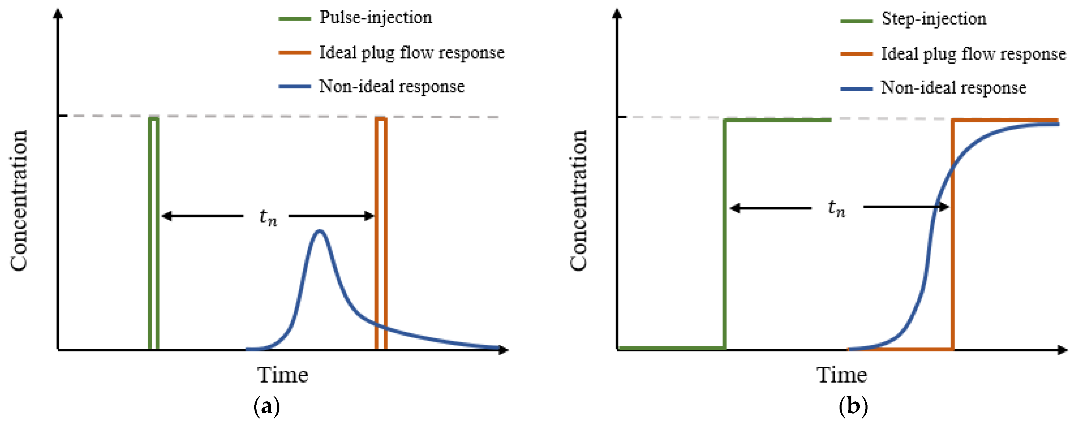
2.1. The Methodology of Tracer Studies

There are two primary approaches to inject the tracer: Pulse-injection and step-injection [40]. Figure 1 illustrates the tracer concentration response corresponding to each of the two input methods, including both ideal and non-ideal conditions.

Pulse injection, also known as slug injection, involves introducing a discrete, concentrated amount of tracer is introduced into the system in a short burst or “pulse”. This creates a distinct pulse of tracer that moves through the system, allowing researchers to track its dispersion and migration over time [41]. As shown in Figure 1, the tracer concentration response over time represents the RTD of the reactor. It reveals the probability of a water particle spending a particular duration in the reactor, providing insights into the system’s mixing characteristics and flow dynamics [42]. In achieving ideal plug flow within CWs (Figure 1a), it is assumed that all fluid parcels move through the wetland with uniform velocity and exit simultaneously. This ideal condition is described by the nominal residence time $t_n$. While in the non-ideal state, it is normal distribution (Gaussian) because of the complex porous structure of CWs and the occurrence of short-circuiting. Certain water particles may exit the system earlier or later. If the shape of the RTD curve has two or more peaks, it can signify the existence of extensive dead zones or bypass zones [32]. For the step-injection method, a constant rate of tracer is continuously introduced into the wetland system, starting at time “0”. Effluent tracer concentration is then regularly monitored at specified intervals until reaching a stable state, indicated by the outlet concentration matching that of the inlet [43]. Figure 1b illustrates the concentration response over time typically observed both at the inlet and outlet during step-injection tracer tests.

Pulse-injection offers simplicity, speed, and wide applicability, making it suitable for experiments that require straightforward and rapid tracer introduction. It is clear theoretical basis facilitates easy analysis and interpretation. However, pulse injection is limited by its discontinuous nature, which may not fully replicate real-world fluid injection processes, and it is susceptible to significant influence from system disturbances, leading to potential errors, especially in unstable systems.

Conversely, step injection offers advantages such as stability, closer simulation to reality, and error reduction. Its continuous tracer injection method helps to stabilize the system, reducing the impact of system disturbances on experimental results. Additionally, step injection closely mimics actual fluid injection processes, resulting in more accurate simulations of real systems. Despite these benefits, step injection requires a more complex experimental setup and data processing compared to pulse injection, demanding greater technical expertise and resources [44]. Therefore, the choice between pulse and step injection depends on the specific experimental objectives, system characteristics, and available resources. It is noteworthy that all hydraulic studies of CWs in the past decade (Table 1) have used pulse injection as the injection method, except for one study that used heat as a tracer for step injection [15].

2.2. Selection of Tracer

When selecting a tracer, it is essential to consider several key requirements. The tracer must be non-toxic and harmless, easily detectable, conservative, representative of fluid behaviour, economically viable, and applicable to the research objectives and system under study [45,46]. By meeting these criteria, the chosen tracer ensures the accuracy, reliability, and safety of experimental results in hydraulic studies. Common tracers used in the field of CWs include but not limited to sodium chloride [27], bromide [34], and fluorescent dyes [33].

2.2.1. Sodium Chloride

Sodium chloride (NaCl), also known as salt tracers, is one of the most common tracers that has been used in many CW hydraulic studies. In recent years, it has often been used to study the clogging effects of CWs [8,9,24,25]. In these studies, the researchers determined the tracer concentration at the outlet of the system by measuring the Electrical Conductivity (EC) at the outlet of the CW and based on a linear correlation between the EC and the NaCl concentration. Lavrnic et al. [27] used NaCl as the tracer to conduct a ponded infiltration test to estimate the saturated hydraulic conductivity ($K_s$) of the surface soil layer at the point scale. Beebe et al. [28] used NaCl to evaluate the impact of evapotranspiration on the performance of CWs and underscores the significance of plant transpiration on vertical transport of constituents.

While salt tracers offer advantages in terms of cost, detectability, and environmental safety, they also present several limitations. In environments with pre-existing salt concentrations, background interference may impede tracer detection, complicating data analysis [47]. Furthermore, salt tracers exhibit limitations in their discriminatory ability, as they lack specificity, hindering the detailed understanding of the behaviour or fate of specific substances within a system [48]. Additionally, due to their high mobility in porous media, salt tracers can rapidly disperse and dilute, especially in highly permeable systems, potentially affecting the accuracy of tracer studies [20]. Therefore, researchers should carefully consider their limitations and potential sources of error when designing tracer experiments.

2.2.2. Fluorescent Dye

Rhodamine WT (RWT) is one of the most commonly used rhodamine derivatives, which is frequently employed as a tracer in environmental studies. RWT exhibits strong fluorescence properties, allowing for easy detection even at concentrations as low as 0.1 parts per billion [32]. Guo et al. [49], used RWT to evaluate the design parameters on the hydraulic performance and treatment efficiency of CWs through orthogonal tests. This study highlighted significant correlations between various hydraulic and purification indicators, as well as a notable correlation between hydraulic efficiency and treatment capacity. In our prior research [31], RWT fluorescent dye was chosen as the tracer to investigate the hydraulic behaviour of an HSFCW under different baffle configurations (i.e., number and length of baffles). The results successfully characterized the RTD of the system, and the average tracer recovery for the five tracer tests was 83.39%. This is a satisfactory recovery rate, thus proving that RWT is an effective tracer that can be used in CWs.

Another commonly used fluorescent dye tracer is uranine. Aylward et al. [36] evaluated the hydraulic efficiency of a start-up, pilot-scale HSFCW located at the Helmholtz UFZ in Leipzig. The study explored the effects of different flow rates and climatic factors on the system. Impulse–response tracer tests were conducted using uranine as the tracer at various depths and locations within the wetland. Volumetric flow rates were closely monitored, and climatic data were collected to support the hydraulic analysis. Pálfy et al. [35] utilized uranine as a tracer to evaluate the hydraulic performance of a CW treating combined sewer overflow. Their findings enabled the researchers to pinpoint short-circuiting as a constraint within the CWs.

Fluorescent tracers offer powerful capabilities for studying hydraulic behaviour and elements distributions in CWs. However, these tracers have certain limitations. They can adsorb onto specific materials within the system, which can alter their behaviour and reduce accuracy. Additionally, fluorescent tracers are susceptible to breaking down under light exposure and degradation due to microbial activity and pH sensitivity. These factors can affect the reliability and effectiveness of the tracer in experiments [50].

2.2.3. Bromide

Bromide is also well-suited for use as a tracer due to its conservative behaviour in water systems. Ávila et al. [37] used potassium bromide as the tracer to investigate the hydraulic efficiency of a three-stage hybrid CW. A major storm event was simulated by increasing the HLR tenfold for one hour to assess the system’s buffer capacity. Birkigt et al. [3] performed a multi-tracer test (deuterium oxide, uranine, and bromide) combined with a mathematical model to explore the flow into the pilot-scale HSFCW in three dimensions due to their different diffusion coefficient. In another study [46], hydraulic tracer tests were conducted to assess the suitability of RWT and bromide as tracers for wetland studies. The study aimed to determine the RTD of the wetlands. The performance of RWT was evaluated by comparing its breakthrough curve to that of bromide in a pilot-scale test, allowing researchers to assess the effectiveness and reliability of RWT as a tracer in wetland environments. The results showed that the time taken to reach 10% and 90% recovery was essentially the same for both tracers. The consistency observed in the RTDs between RWT and bromide suggests that bromide is a suitable tracer for CWs tracer tests.

2.2.4. Alternative Tracer Options

Although the tracer categories mentioned previously are widely used, additional alternatives, including fluoride, propane gas, and heat mapping, have been utilized in various studies. Munavalli et al. [39] used fluoride as the tracer to evaluate the hydraulic efficiency and to assess the treatment efficiency of an HSFCW under different HLRs. The tracer study and associated calculations demonstrated the effective hydraulic performance of the system. Decezaro et al. [51] introduced the gas tracer method for evaluating the oxygen transfer capacity of a real-scale VSFCW treating domestic wastewater. Propane was employed as the tracer, and the Oxygen Transfer Rate (OTR) was assessed under HLR of 60, 90, and 120 mm d⁻¹, corresponding to recirculation ratios of 0%, 50%, and 100%. The results revealed that the OTR in standard conditions (20 °C) ranged from 120 to 176 g O2 m⁻² d⁻¹, with the highest OTR observed under the lowest HLR. In another study [15], Bonner et al. proposed using heat as an eco-friendly alternative to chemical tracers in wetland studies. They developed a mapping methodology that converts heat tracer response curves into conservative chemical tracer responses. Testing on a laboratory-scale wetland showed close alignment between predicted and actual chemical tracer responses, with only a 5% and 6% relative difference in the Peclet number and mean of the RTD, respectively.

2.2.5. Practical Considerations and Uncertainties in Tracer Application

While tracer experiments are a powerful tool for understanding hydraulic behaviour in CWs, their practical implementation involves a number of considerations that can affect data accuracy and interpretation.

Each tracer type presents specific operational advantages and challenges (shown in

Table 2. Comparison of different tracers used in hydraulic studies of CWs.

Tracer Type	Advantages	Limitations	Typical Applications
Dye tracer (e.g., Rhodamine WT)	Easy to detect; cost-effective; low toxicity; widely available	Subject to photodegradation; adsorption to media may occur	Small- to medium-scale CWs
Salt tracer (e.g., NaCl)	Inexpensive; chemically stable; easy to measure via conductivity	Affected by background salinity; less suitable in saline environments	Field studies; systems with low background conductivity
Bromide (e.g., KBr)	Conservative tracer; minimal interaction with substrate or biota	Requires laboratory analysis (ion chromatography); more costly	Research-grade CW studies
Heat mapping (e.g., thermal tracer)	Non-invasive; visualizes temperature-based flow patterns	Low spatial resolution; affected by ambient temperature	Surface or shallow subsurface CWs

). For example, Rhodamine WT offers high detection sensitivity, allowing for low-concentration usage and minimal environmental impact, but it is vulnerable to photodegradation and adsorption onto organic substrates. Sodium chloride is widely used due to its low cost and simple conductivity-based detection; however, it is prone to background interference in saline environments and tends to rapidly dilute in highly permeable media. Bromide is considered conservative and chemically stable, but it requires laboratory analysis and can be cost-prohibitive in large-scale applications.

Tracer recovery rates are influenced by several factors that introduce uncertainty into hydraulic assessments. Vegetation density can alter flow paths and increase tracer dispersion due to root zone heterogeneity. Clogging or sediment accumulation may induce dead zones or preferential pathways, leading to underestimation or overestimation of residence time. Incomplete recovery of tracer mass at the outlet—whether due to adsorption, degradation, or unmonitored lateral loss—can also impair RTD curve accuracy.

Real-world case studies have demonstrated both the utility and limitations of tracer experiments. In a previous study by the authors [31], the use of Rhodamine WT in a baffled HSFCW yielded a tracer recovery rate of 83.39%, which was deemed acceptable but highlighted some loss due to adsorption or plant uptake. Similarly, Pálfy et al. [35] applied uranine in a CW treating combined sewer overflow, successfully identifying short-circuiting as a key performance limitation. These examples show how tracer data not only quantifies hydraulic efficiency but also informs targeted design interventions, such as baffle addition or inlet redesign.

Additionally, numerical validation using tracer-derived RTD curves also improves model calibration. CFD simulations, for instance, can be adjusted to match observed tracer breakthrough curves, enhancing the reliability of flow predictions and design outcomes. Thus, combining field tracer studies with modelling approaches strengthens the scientific basis for wetland design optimization.

2.3. Index for Hydraulic Performance Assessment in CWs

The hydraulic performance indexes are derived from the RTDs to assess the hydraulic performance of the system. It usually can be divided into three categories: hydraulic efficiency indexes (HEIs) ($e,\lambda$, and $MI$), short-circuiting indexes (SIs) ($t_5$ and $t_{10}$), and mixing indexes (MIs) (${\sigma }^2$, ${\sigma }_{\theta }^2,N,$ and MDI) [52,53].

The RTD function quantifies the duration fluid particles spend within the reactor. This function can be derived from the tracer concentration at the outlet over time and is expressed as

$$E(t)={\displaystyle \frac{Q\left(t\right)C\left(t\right)}{{\int }_0^{\mathrm{\infty }}Q\left(t\right)C\left(t\right)dt}}$$

(1)

where $Q\left(t\right)$ represents the flow rate at time t, $C\left(t\right)$ is the tracer concentration at the outlet at time t, and $dt$ indicates the sampling time interval.

Mean residence time $t_m$ is the first moment of the RTD function, also known as actual residence time, representing the actual average duration of a tracer particle remains in the CWs system. $t_m$ is the determinant factor hydraulic efficiency of CWs. It is typically used to quantify the efficiency by dividing it by the nominal residence time $t_n$, indicating the ratio of the effectively used volume to the total volume of the system in the wetland [54]. They can be calculated using the Equations (2) and (3), respectively:

$$t_m={\int }_0^{\mathrm{\infty }}t\cdot E\left(t\right)dt$$

(2)

$$e={\displaystyle \frac{t_m}{t_n}}$$

(3)

The variance ${\sigma }^2$ is mathematically defined as the second moment of the E(t) curve relative to $t_m$, indicating the spread of the RTD function. It is computed as Equation (4):

$${\sigma }^2={{\int }_0^{\mathrm{\infty }}\left(t-t_m\right)}^{2}E\left(t\right)dt$$

(4)

The TIS model describes non-ideal flow behaviour in reactors. It views a reactor as a series of equal-volume Continuous Stirred Tank Reactors (CSTRs), with N representing the number of CSTRs. As N increases, the system approaches ideal plug flow reactor (PFR), while N equal to one indicates completely mixed flow [19]. The TIS model adjusts N to simulate different flow behaviours, aiding in reactor design optimization and fluid flow analysis. Persson et al. [42] proposed that the number of tanks in series N can be expressed as

$$N={\displaystyle \frac{t_m^2}{{\sigma }^2}}={\displaystyle \frac{1}{{\sigma }_{\theta }^2}}$$

(5)

where ${\sigma }_{\theta }^2$ is the dimensionless variance, which has also been used to indicate local mixing in some studies [13,26,34].

Persson et al. [7] proposed that the hydraulic efficiency $\lambda$ can be assessed by combing the flow uniformity and the effective volume of the wetland system, which can be expressed by Equation (6):

$$\lambda =e\left(1-{\displaystyle \frac{1}{N}}\right)=\left({\displaystyle \frac{t_m}{t_n}}\right)\left(1-{\displaystyle \frac{t_m-t_p}{t_m}}\right)={\displaystyle \frac{t_p}{t_n}}$$

(6)

where $t_p$ is the time point of the peak on the RTD curve.

This index quantifies the extent to which inflow is evenly distributed across the entire cross-section of a wetland, offering a comprehensive reflection of the impact of short-circuiting and mixing on the hydraulic performance of a CW. According to the study [7], the hydraulic efficiency of CWs can be grouped into three categories based on their value: good hydraulic efficiency when λ > 0.75, satisfactory efficiency when 0.5 < λ ≤ 0.75, and poor efficiency when λ ≤ 0.5.

In addition to these common hydraulic indexes mentioned above, some optimal hydraulic indexes have been proposed for enhanced suitability in recent years. Sun et al. [11] demonstrated that the index S (Equation (7)) provides the most reliable measure of short-circuiting, as it correlates closely with advective flow, exhibits minimal statistical variability, and effectively indicates channelling throughout the system.

$$S={\displaystyle \frac{t_{10}}{t_n}}$$

(7)

where $t_{10}$ represents the time taken for the initial 10% of the injected tracer mass to reach the outlet of the system. A smaller value of $S$ indicates a higher degree of short-circuiting or channelling through the system.

The RTD’s variance ${\sigma }^2$ stands out as the optimal metric for gauging mixing impacts, owing to its intimate link with the underlying physical processes and its prevalent adoption across various kinetic models [55]. When the value of ${\sigma }^2$ decreases, it indicates a narrower spread of the data and a reduced degree of mixing. However, this index is limited by its high statistical variability when mixing effects are minimal.

When mixing is minimal, the Morril Dispersion Index (MDI) (Equation (8)) is preferred [20,36]. A higher MDI value indicates an extended duration for the majority of material to exit the system and signifies a greater degree of mixing.

$$MDI={\displaystyle \frac{t_{90}}{t_{10}}}$$

(8)

where $t_{90}$ represents the time required for 90% of the injected tracer mass to reach the system outlet.

Moreover, a novel HEI known as the moment index ($MI$) (Equation (9)), introduced by [56], offers several advantages. Firstly, $MI$ accounts for both short-circuiting and mixing effects while remaining independent of them. Secondly, unlike other indexes, $MI$ is not influenced by the long tail of the RTD curve. The calculation formula of $MI$ (Equation (9)) yields values within the range of 0 to 1. It is important to note that, according to the definition of $MI$, the normalization of the RTD is based on the mass of added tracer rather than the mass of recovered tracer.

$$MI=1-{\int }_0^1\left(1-\phi \right)f\left(\phi \right)d(\phi )$$

(9)

where $\phi$ is a normalized dimensionless variable of $t$ for comparison of different CWs’ RTDs. $\phi$ and $f\left(\phi \right)$ can be expressed as

$$\phi ={\displaystyle \frac{t}{t_n}}$$

(10)

$$f\left(\phi \right)={\displaystyle \frac{c\left(\phi \right)V}{M}}$$

(11)

where $V$ is the volume of water in system, $M$ is the total mass of recovered tracers.

For the above hydraulic indexes, some studies have a different perspective. Guo et al. [12] argued that using the degree of plug flow or completely mixed flow alone is insufficient for assessing hydraulic performance. They also advised against using the number of tanks “N” in the TIS model as an evaluation parameter due to its instability and significant truncation effect. These parameters merely indicate deviations from the plug flow pattern without revealing the actual water current conditions. Consequently, they did not recommend hydraulic efficiency $\lambda$ as a suitable indicator for hydraulic performance. Instead, they emphasized the effective volume ratio $e$, short-circuiting index $t_{10}$, and mixing index MDI as the most important and reasonable parameters for assessing the hydraulic performance of subsurface flow CWs. Similarly, Liu et al. [53] also recommended using $t_{10}$ and MDI as indicators for evaluating the hydraulic performance of CWs. However, hydraulic efficiency $\lambda$ was considered to be equally reliable.

2.4. Water Quality Responses of CWs to Changing Hydrological Conditions

As mentioned before, poor flow behaviour in CWs affects the amount of effective contact surface between pollutants and the biofilm. Thus, there exists a strong correlation between the hydraulic performance of CWs and their treatment efficiency [7,57].

Kusin et al. [29] conducted tracer tests to assess hydraulic performance and its impact on iron removal in CWs and lagoons. Results indicated a correlation between hydraulic efficiency, as determined by the TIS model, and iron retention. Specifically, wetlands exhibited a mean hydraulic efficiency of 69%, compared to 24% for lagoons. Iron treatment efficiency was 81% and 47% for wetlands and lagoons, respectively. Enhancing treatment system performance may involve maximizing hydraulic efficiency by increasing residence time and ensuring uniform flow movement. Cakir et al. [58] investigated the correlation between the hydraulic loading rate and treatment performance of an HSFCW. Three chambers, varying in hydraulic loading rates (0.050, 0.075, and 0.125 m³/day/m²), were planted with Phragmites australis. The results indicated that removal efficiencies were influenced by hydraulic loading rate, with the highest rates observed at 0.050 m³/day/m²: 64.9% for Biochemical Oxygen Demand (BOD₅), 62.5% for Chemical Oxygen Demand (COD), 86.3% for Total Suspended Solids (TSSs), and 80.34% for Oil and Grease. Tee et al. [59] conducted a study comparing the effectiveness of baffled and traditional HSFCWs in removing nitrogen at hydraulic retention times (HRTs) of 2, 3, and 5 days. The baffled unit with plants demonstrated superior performance, achieving higher ammonia–nitrogen removal rates of 74%, 84%, and 99%, compared to 55%, 70%, and 96% in the conventional unit at the corresponding HRTs. The researchers noted that the extended hydraulic path in the baffled CW enhanced wastewater interaction with the rhizome and microaerobic zones, resulting in improved pollutant removal efficiency. Wang et al. [26] obtained consistent results, indicating a 42.6% improvement in hydraulic efficiency with the addition of baffles. This resulted in increased pollutant removal rates and reduced negative impacts from shock loads.

However, there are also studies indicating that improvements in hydraulic behaviour do not necessarily result in enhanced treatment efficiency. For example, during 2016 and 2017, Marzo et al. [25] evaluated the hydraulic behaviour of an HSFCW using multiple methods, including measurements of hydraulic conductivity at saturation (Ks), tracer tests, and geophysical techniques such as electrical resistivity tomography. The findings revealed clogging at the inlet; however, partial clogging did not diminish the system’s capacity for removing organic matter and suspended solids.

Despite the two different opinions, the effect of hydraulic performance of CWs on HRT cannot be ignored. Short-circuiting, which leads to a shorter HRT, can result in incomplete treatment of the wastewater. While extending HRT in CWs typically slows the passage of wastewater through the beds, accomplished by employing low HLR. This facilitates extensive interactions among wastewater constituents, the rhizosphere, and microbial communities. As HRT increases, the removal efficiencies of TSS, COD, BOD₅, and Total Nitrogen (TN) generally improve, although this improvement is subject to a threshold [60]. For example, Xing et al. found that in biochar-based constructed wetlands, the optimal HRT range is between 36 and 48 h. They observed that pollutant removal efficiency initially increased but then declined as the HRT increased to 60 h [61]. This indicates that overly prolonged or short HRT both could reduce wastewater treatment capacity. In a previous study by the authors [62], a baffled HSFCW with five different baffle configurations (0, 1, 3, 5, and 7), each corresponding to a distinct HE was investigated. The results demonstrated that increased baffle numbers—and thus higher HE—led to improved pollutant removal efficiencies: TOC removal increased from 51.09% (0 baffles) to 74.54% (7 baffles), TN from 41.42% to 62.39%, and TP from 46.84% to 59.46%. These findings highlight how hydraulic behaviour, shaped by wetland configuration, directly influences treatment capacity. A higher HE positively influences pollutant removal rates in HSFCWs, as the mean residence time of pollutants more closely matches the design value. By increasing the contact time between pollutants and wetland media, such as substrates, plant roots, and microbial biofilms, the system’s pollutant removal efficiency is significantly improved. Additionally, short-circuiting and dead zones, common in systems with poor internal hydraulics, reduce the effective volume of the wetland and lead to insufficient treatment. Wastewater bypasses critical treatment zones, resulting in lower removal efficiencies and greater sensitivity to inflow fluctuations.

Therefore, the improvement of hydraulic efficiency undoubtedly contributes to treatment efficacy, albeit to varying degrees. This may be affected by factors such as the type and scale of the wetland, pollutant influent loads, the climatic conditions, amongst other variables.

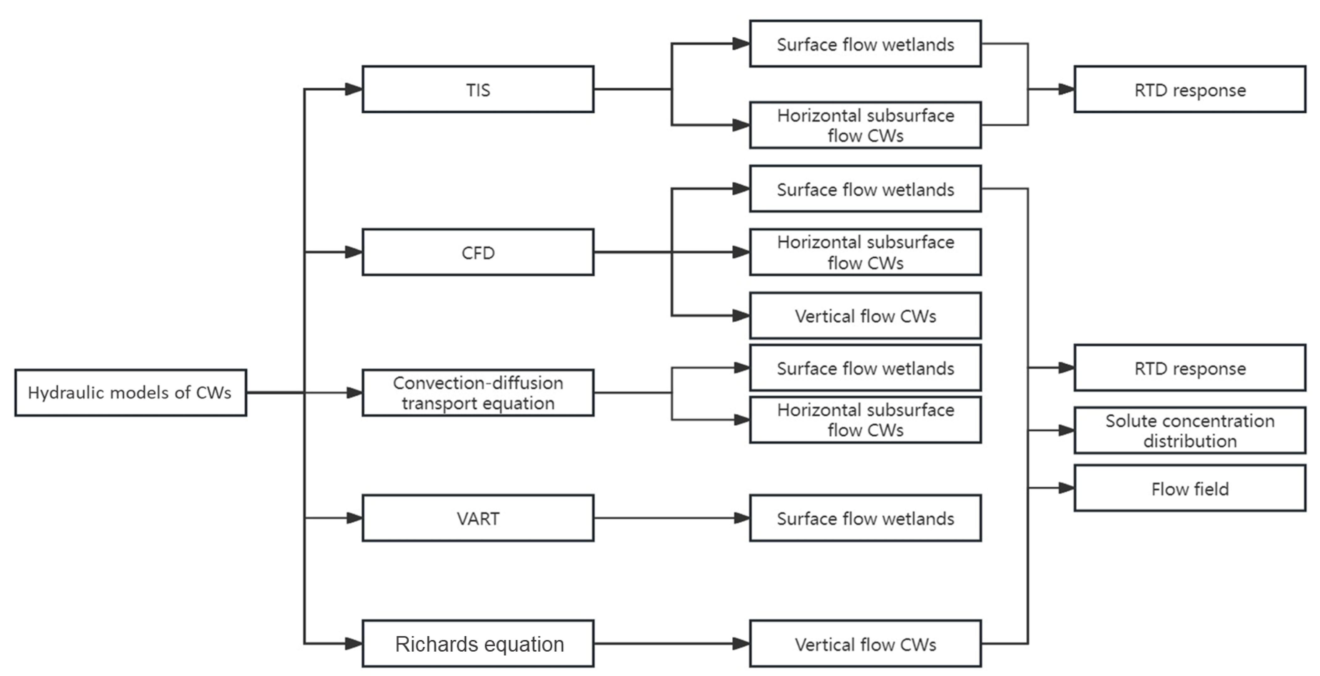
3. Numerical Models for Hydraulic Studies in CWs

Numerical models are also valuable tools for interpreting and analysing the RTD, providing insights into flow patterns, pollutant transport, and system performance [14].

3.1. Tank-in-Series Model

Models that describe the RTD functions of CWs often use concepts originally developed in chemical engineering to clarify flow patterns in reactors [63]. The Plug Flow Reactor (PFR) and the Completely Stirred Tank Reactor (CSTR) are two widely used ideal models [20,30]. However, the actual fluid patterns in CWs are non-ideal, falling somewhere between PFR and CSTR due to the complex flow paths caused by the wetland structure, substrates, and vegetation [64].

This systemic modelling approach has been extensively applied to simulate the hydraulic behaviour of CWs [2,10,30]. It involves describing the flow behaviour through a combination of interconnected elementary reactors, such as the PFR, the CSTR, and the Plug Flow with Dispersion (PFD) model [63]. The most commonly used model is the TIS model to represent gradual mixing in CWs. In this model, the wetland system is conceptualized as a sequence of CSTRs arranged in series. The dynamics of tracer concentrations within this system are governed by a set of differential equations that describe the mixing and transport processes [65]:

$$\left\{\begin{array}{c}{\displaystyle \frac{\tau }{N}}{\displaystyle \frac{dc(1,t)}{dt}}=x\left(t\right)-c\left(1,t\right), i=1\\ {\displaystyle \frac{\tau }{N}}{\displaystyle \frac{dc(i,t)}{dt}}=c\left(i-1,t\right)-c\left(i,t\right),i=\mathrm{2,3},\dots ,N\end{array}\right.$$

(12)

where $\tau$ represents the total retention time, $N$ represents the number of CSTRs, also can be expressed by Equation (5), $x\left(t\right)$ is the function of inlet tracer concentration, and $c\left(i,t\right)$ is the outlet concentration of the $i$th CSTR.

Equation (12) allows for an analytical solution when introducing a Dirac delta function as the tracer pulse input. This analytical solution yields the effluent concentration from the final tank, $N$, which represents the RTD function for the TIS model, as detailed in Equation (13) [65]:

$$f_{TIS}\left(t\right)=c\left(N,t\right)={\displaystyle \frac{N^n{t}^{N-1}}{{\tau }^N\left(N-1\right)!}}\mathrm{e}\mathrm{x}\mathrm{p}({\displaystyle \frac{-Nt}{\tau }})$$

(13)

Wang et al. [26] conducted a series of tracer studies and used the TIS model to evaluate the hydraulic performance of six different types of small-scale CWs. The findings demonstrate that the TIS model exhibits a superior fit to the RTD of six distinct types of CWs. The peak value, time to reach the peak, and slope of the fitted curve closely resemble the measured RTD. Kusin et al. [29] analysed the tracer RTD based on the TIS model to yield the mean residence time and corresponding hydraulic characteristics of a wetland and a lagoon. The results indicate a correlation between system hydraulic efficiency, derived from the TIS model principle, and iron retention in the treatment systems.

Considering the applications of the TIS model, it is important to note that this model is conceptual in nature. It characterizes flow behaviour through the combination of elementary reactors instead of directly calculating the flow field. While systemic models offer valuable insights into global hydrodynamic characteristics like RTD, they often lack detailed information on local flow conditions. Furthermore, systemic models are known for their simplicity and computational efficiency, but their ability to accurately predict outcomes beyond the scope of observed data is limited [66].

Compared to more complex simulation approaches such as CFD, the TIS model is relatively easy to implement and requires minimal computational resources. However, it provides only macroscopic representations of flow without resolving detailed velocity fields or spatial heterogeneity.

3.2. Computational Fluid Dynamics (CFD) Modelling

CFD modelling is also a valuable tool that has been widely used to simulate the complex flow behaviour in CWs [67,68]. This method involves the use of computational grids to discretize the geometry. In CFD simulations, the flow within the system is governed by the continuity equation (Equation (14)) and the momentum equation (Equation (15)). The Darcy–Forchheimer model (Equation (16)) is incorporated as a momentum loss source term ($S_i$) in the momentum equation to simulate the hindering effect of the substrates on the internal fluid flow, thereby describing fluid flow through porous media in CWs [69]. The fluid domain is spatially averaged during the solution of the porous media model [8].

$${\displaystyle \frac{\partial \rho }{\partial t}}+{\displaystyle \frac{\partial \left(\rho ui\right)}{\partial xi}}=0$$

(14)

where $\rho$ is the fluid density, $ui$ is the fluid velocity in the $i$-direction, $x_i$ is the spatial coordinate in the $i$-direction, and the subscript i = 1, 2, 3.

$${\displaystyle \frac{\partial \left(\rho ui\right)}{\partial t}}+{\displaystyle \frac{\partial }{\partial x_j}}\left(\rho ujui\right)=-{\displaystyle \frac{\partial p}{\partial xi}}+{\displaystyle \frac{\partial }{\partial x_j}}\left({\tau }_{ij}+{\tau }_{tij}\right)+\rho g_i+f_{\sigma i}+S_i$$

(15)

in which $ui$ and $uj$ represent the velocity in the $i$- and $j$-direction, respectively; $x_i$ and $x_j$ are the spatial coordinates in the $i$- and $j$-direction, respectively; $p$ is the pressure, ${\tau }_{ij}$ and ${\tau }_{tij}$ are the viscous and turbulent stress. Since the flow in CWs is generally laminar (Re < 600) [22]; ${\tau }_{tij}$ equals 0. $g_i$ is the gravitational acceleration; $f_{\sigma i}$ is the surface tension.

$$S_i=-\left(C_1{\mu u}_i+C_2{\displaystyle \frac{1}{2}}\rho \left|u_i\right|u_i\right)$$

(16)

where $\mu$ is the fluid viscosity, and the coefficients C1 and C2 are calculated by solving the following equations [70]:

$$C_1={\displaystyle \frac{150}{d_p^2}}{\displaystyle \frac{{\left(1-\epsilon \right)}^2}{{\epsilon }^3}}$$

(17)

$$C_2={\displaystyle \frac{3.5}{d_p}}{\displaystyle \frac{\left(1-\epsilon \right)}{{\epsilon }^3}}$$

(18)

in which $d_p$ is the mean particle size of the filter, and $\epsilon$ is the porosity of the substrates.

In recent years, CFD modelling has been mainly used to explore the effects of changes in design parameters, including inlet–outlet configuration [5], baffle configuration [71], vegetation distribution [72], and clogging effects [8,9]. The RTD was obtained from the numerical simulation of flow fields and monitoring the variation of tracer concentration over time at the outlet [31].

In contrast to the conceptual nature of the TIS model, CFD offers a detailed, spatially resolved understanding of fluid movement and mixing patterns within CWs. This allows researchers to visualize flow anomalies, dead zones, and preferential pathways that would be difficult to detect using lumped models. However, CFD simulations are computationally intensive and require significant expertise in model setup, calibration, and validation. Therefore, while the TIS model is more suitable for quick system-level analysis and comparisons, CFD provides higher accuracy and detailed diagnostic capacity, making it more appropriate when system design optimization or internal hydrodynamics are of primary concern.

3.3. The Richards Equation

The Richards equation is a mathematical description used to model the flow of water through unsaturated porous media, such as soil [73]. The equation is a partial differential equation and is expressed as

$${\displaystyle \frac{\partial \theta }{\partial t}}={\displaystyle \frac{\partial }{\partial z}}\left[K\left(({\displaystyle \frac{\partial h}{\partial z}}-1)\right)\right]$$

(19)

where $\theta$ is the volumetric water content, $h$ is the pressure head, $K$ is the unsaturated hydraulic conductivity, z is the vertical coordinate measured downward from the top surface, and $t$ is the time. The variables $\theta$ and $K$, which depend on $h$, can be described using the van Genuchten–Mualem functions [74]:

$$\left\{\begin{array}{c}\theta ={\theta }_r+{\displaystyle \frac{{\theta }_s-{\theta }_r}{{\left(1+{\left|\alpha h\right|}^{1/(1-m)}\right)}^m}},h<0\\ \theta ={\theta }_s,h \ge 0\end{array}\right.$$

(20)

$$\left\{\begin{array}{c}K=K_s{\left({\displaystyle \frac{\theta -{\theta }_r}{{\theta }_s-{\theta }_r}}\right)}^{0.5}\times {\left[1-{\left({1-\left({\displaystyle \frac{\theta -{\theta }_r}{{\theta }_s-{\theta }_r}}\right)}^{{\displaystyle \frac{1}{m}}}\right)}^m\right]}^2,h<0\\ K=K_s,h \ge 0\end{array}\right.$$

(21)

The Richards equation is frequently employed to characterize the flow behaviour in VFSCWs because in these systems, water input and output are typically intermittent, resulting in constantly changing saturation levels [75]. This equation allows for more accurate modelling and prediction of flow dynamics within the wetlands, aiding in the design and management of the systems to enhance their treatment efficiency and stability. Additionally, the Richards equation is a fundamental partial differential equation included in the HYDRUS Wetland model, which is implemented in the HYDRUS software. The HYDRUS software is recognized as one of the most detailed and process-based models available today for simulating water, solute, and heat transport in variably saturated porous media [75].

Ciro et al. [16] proposed a model that combines a first-order kinetic model with advection/dispersion and the Richards equations to predict the removal rates of BOD₅ and TN from domestic wastewater. Samso et al. [76] developed a mathematical model using COMSOL Multiphysics v4.3b and MATLAB (version R2013b) to simulate bio clogging effects in HFSCWs. The model describes variably saturated subsurface flow and overland flow using the Richards equation, providing a detailed simulation of how bio clogging impacts water flow in these systems. The Richards equation offers flexibility by allowing adaptation to various scenarios through the incorporation of different boundary conditions, soil properties, and external influences. This adaptability enables its application across a wide range of soil types and environmental conditions. However, its sensitivity to parameters, including soil hydraulic properties, initial conditions, and boundary conditions, poses a challenge. Inaccurate or uncertain parameter values can result in significant errors in model predictions, highlighting the importance of careful parameter estimation and validation [77].

3.4. Convection–Diffusion Equation

The convection–diffusion equation is widely used by researchers to describe the flow behaviour and solute transport in wetland systems [14,63,78]. Compared to the Navier–Stokes equations in CFD models, the convection–diffusion equation describes the transport of scalar quantities in a flowing fluid by considering both convective and diffusive processes, but does not consider the effects of pressure, viscosity, or inertia on fluid motion. In this methodology, the transport model includes the physical processes of convection and diffusion. Convection is the transfer of solutes in fluids through the bulk movement of the fluid itself. Diffusion, on the other hand, is the process where particles move from an area of higher concentration to an area of lower concentration due to random molecular motion [79].

3.5. Variable Residence Time Model (VART)

The VART model, developed by Deng et al. [80], simulates solute transport in natural streams with transient storage and release effects. It divides transient storage zones into two sublayers: an upper advection-dominated layer with strong hyporheic exchange and a lower diffusion-dominated layer that extends to the deeper streambed. These two types of transient storage zones bear resemblance to those observed in treatment wetlands [18], particularly in terms of their transient storage effects. This model is useful for predicting solute transport and removal processes in environments similar to treatment wetlands. The VART model was integrated with kinetic processes to form the VART-BOD model [17,81], simulating various BOD₅ removal mechanisms. These include Monod kinetics of bacterial growth, mass exchange between the water column and root layers, as well as advection, dispersion, and diffusion processes.

4. Discussion

Each method discussed in this paper has its own set of advantages and disadvantages. It is important to highlight that using inappropriate methods for hydraulic analysis may result in inaccurately estimating a wetland’s effective volume and dispersion characteristics. Therefore, the selection of a method for hydraulic studies of CWs depends on the specific experimental and simulation objectives, system characteristics, and available resources.

Table 3. Comparison of different models used in hydraulic studies of CWs.

Model	Key Features	Advantages	Limitations	Computational Complexity
TIS	Series of CSTRs approximating RTD	Good fit for RTD; low data requirement	Lacks internal spatial detail	Low
CFD	Solves Navier–Stokes or Darcy–Forchheimer in discretized domain	High spatial resolution; visualizes flow field	High computational demand; needs validation	High
Convection–diffusion	Models transport using advection and dispersion equations	Captures key processes; analytical foundation	Assumes steady-state; limited for 3D, variable flows	Medium
The Richards equation	Governs unsaturated flow through porous media	Suitable for variably saturated zones	Complex parameters; computationally intensive	High
VART	Allows variable residence time in system compartments	Flexible representation of non-ideal flow	Limited availability; calibration challenging	Medium–High

compares the numerical models discussed Section 3, including their key features, advantages, and limitations. In addition to their distinct levels of complexity and predictive capabilities, numerical models differ significantly in computational cost and validation requirements. CFD models offer the highest spatial resolution and predictive power, but they demand substantial computational resources, longer simulation times, and expertise in numerical solvers and mesh generation. In contrast, TIS and convection–diffusion models are computationally lightweight and can be readily applied in field-scale studies, though they provide limited insights into internal flow dynamics.

Validation of numerical models is essential to ensure their reliability in simulating real-world CW systems. Common validation techniques involve comparing model-generated RTD curves against experimental data from tracer studies. For example, parameters in a TIS model are often calibrated using observed breakthrough curves, while CFD models may be validated by matching predicted and observed tracer concentrations at the outlet or by comparing velocity fields with flow visualization results.

Figure 2 illustrates the types of CWs suitable for different hydraulic models. Due to the high flexibility and adjustability of CFD modelling, along with its inclusion of turbulent and laminar flow models, it can be applied to simulate the complex water flow behaviour in all types of CWs. TIS model typically divides the subject of study into sequential flow compartments. Therefore, it is suitable for simulating the flow behaviour and mixing within HSFCWs and SFWs. Each tank represents a segment of the wetland where water moves sequentially, allowing for the analysis of retention time and mixing efficiency. The Convection–Diffusion Transport Equation is also a good choice for HSFCWs and SFWs. These two wetland types rely on water movement across the surface, where solutes are transported primarily through advection and diffusion. The convection–diffusion equation provides a mathematical framework for modelling these transport processes, considering factors like flow velocity, diffusion coefficients, and concentration gradients. Another hydraulic model option for SFWs is VART. This model divides flow areas into two sublayers, each governed by different mechanisms of solute transport. The upper layer illustrates a transient storage zone primarily influenced by advection, characterized by notable hyporheic exchange of solutes. In contrast, the lower layer represents an effective storage zone primarily governed by diffusion, encompassing the deeper stream bed extending to the banks. This accounts for vertical flow non-uniformity and water retention effects, thereby enhancing the accuracy of water movement simulation in SFWs. In cases where flow is unsaturated, as commonly observed in VSFCWs, the Richards equation would be the preferred hydraulic model.

If the goal of the research is to explore the impact of altering design parameters on the hydraulic performance of a CW, then CFD modelling would be the preferred choice due to its flexibility in modifying boundary conditions and adjusting initial conditions. Alternatively, if the focus is on studying how altering design factors affects the system effective volume utilization, then the TIS model would be suitable. To model the purification of pollutants in the CW system and understand the impact of hydraulic performance on this process, researchers can use the convective–diffusive model, the VART model, or the Richards equation. These models often integrate with biokinetic models, which describe the biological processes involved in contaminant degradation, such as microbial activity. Consequently, researchers can gain comprehensive insights into both the physical transport and biological degradation of contaminants in wastewater.

In terms of system characteristics, the physical and chemical properties of the substrate, such as particle size, specific surface area, porosity, permeability coefficient, etc., are considered sensitive factors in tracer studies. These factors affect the transport and adsorption behaviour of tracers in the medium, thereby influencing the reliability of experimental results. Previous studies [82] have demonstrated that substrate adsorption is the primary reason for a low tracer recovery rate. For numerical models, Llorens et al. [83] found that changes in the longitudinal dispersion coefficient significantly affected the model’s performance and accuracy. A similar result was found by Langergraber et al. [77], they demonstrated that the longitudinal dispersion coefficient had the greatest impact on the simulation outcomes, making it the most influential parameter in their hydraulic model.

Because of the complex and variable water flow patterns of CWs, results obtained solely through tracer methods or modelling are often uncertain and impractical. Therefore, it is necessary to combine both methods to jointly assess the hydraulic behaviour in CWs. Many studies have demonstrated that combining tracer experiments and numerical modelling is a good choice to improve the reliability of the study and allows the model to be effectively used to aid in design purposes before the system is constructed [3,9,11,31].

Currently, there is a lack of research that combines hydraulic modelling and pollutant removal modelling in an integrated modelling approach. Moreover, the potential impacts of fully controlling or intervening in hydraulic processes to enhance pollutant removal efficiency on other ecological functions of CWs are unclear. This is due to a lack of understanding regarding the responses of hydraulic, water quality, and biological components of different CWs to hydrological changes.

Integrating hydraulic models with pollutant removal models presents a promising direction for more accurately simulating and optimizing CW performance. Hydraulic models such as CFD or TIS can be coupled with kinetic models that simulate biochemical reactions (e.g., first-order kinetics, Monod kinetics) to dynamically reflect how flow conditions affect contaminant transformation and degradation.

However, this integration poses several challenges, including the need for consistent spatial and temporal scales between the models, increased computational complexity, and the requirement for high-quality calibration data across multiple physical, chemical, and biological domains.

Despite these challenges, a few studies have demonstrated successful integration. Ciro et al. [16] proposed a model that combines a first-order kinetic model with advection/dispersion and the Richards equations to predict the removal rates of BOD₅ and TN from domestic wastewater. Similarly, the VART model was integrated with kinetic processes to form the VART-BOD model [17,81], simulating various BOD₅ removal mechanisms. These examples highlight the feasibility and benefits of integrated models in capturing interactions between hydrodynamics and treatment processes.

Therefore, in future research, the hydraulic studies of CWs should include:

(a)

Integration with biochemical reaction kinetic models to simulate pollutant degradation under realistic flow conditions;

(b)

Quantitative analysis of the relationship between hydraulic efficiency and pollutant removal efficiency for specific target parameters;

(c)

Development of comprehensive, multi-process models capable of simulating the coupled hydraulic–biochemical behaviour of CWs;

(d)

Adoption of machine learning (ML) and AI techniques (e.g., neural networks, genetic algorithms, and surrogate modelling) to improve predictive accuracy, automate parameter calibration, and identify key design variables influencing treatment performance under varying hydraulic conditions.

5. Conclusions

The tracer methods and diverse numerical models discussed in this paper offer various approaches for analysing the hydraulic behaviour of CWs. Selecting the right method and suitable indexes for assessment is crucial, considering specific experimental goals, system characteristics, and available resources to avoid inaccuracies in wetland effectiveness estimation.

For horizontal subsurface flow CWs, the TIS model and the Richards equation are suitable, offering insights into flow behaviour and soil water dynamics, respectively. Vertical subsurface flow CWs benefit from CFD and VART models, providing detailed flow pattern simulations and transient storage effects consideration. Surface flow wetlands can be effectively analysed using the Convection–Diffusion Transport Equation and the TIS model.

Future research should focus on integrating hydraulic models with biochemical kinetics to better simulate pollutant degradation processes under realistic flow conditions. Quantitative investigations into the link between hydraulic efficiency and treatment performance are essential for identifying optimization strategies. Furthermore, the development of comprehensive, multi-process models—potentially supported by machine learning and AI—will enhance the predictive accuracy and adaptability of CW design across scales and environments.

By aligning hydraulic modelling with pollutant removal goals and incorporating advanced tools, future work can significantly contribute to the sustainable design, operation, and upscaling of constructed wetlands as nature-based solutions for long-term wastewater management.

References

1. Stottmeister, U.; Wiessner, A.; Kuschk, P.; Kappelmeyer, U.; Kastner, M.; Bederski, O.; Muller, R.A.; Moormann, H. Effects of plants and microorganisms in constructed wetlands for wastewater treatment. Biotechnol. Adv. 2003, 22, 93–117. [Google Scholar] [PubMed]
2. Laurent, J.; Bois, P.; Nuel, M.; Wanko, A. Systemic models of full-scale Surface Flow Treatment Wetlands: Determination by application of fluorescent tracers. Chem. Eng. J. 2015, 264, 389–398. [Google Scholar]
3. Birkigt, J.; Stumpp, C.; Maloszewski, P.; Nijenhuis, I. Evaluation of the hydrological flow paths in a gravel bed filter modeling a horizontal subsurface flow wetland by using a multi-tracer experiment. Sci. Total Environ. 2018, 621, 265–272. [Google Scholar] [PubMed]
4. Stephenson, R.; Sheridan, C.; Kappelmeyer, U. A curve-shift technique for the use of non-conservative organic tracers in constructed wetlands. Sci. Total Environ. 2021, 752, 141818. [Google Scholar]
5. Sabokrouhiyeh, N.; Bottacin-Busolin, A.; Savickis, J.; Nepf, H.; Marion, A. A numerical study of the effect of wetland shape and inlet-outlet configuration on wetland performance. Ecol. Eng. 2017, 105, 170–179. [Google Scholar]
6. Wahl, M.D.; Brown, L.C.; Soboyejo, A.O.; Dong, B. Quantifying the hydraulic performance of treatment wetlands using reliability functions. Ecol. Eng. 2012, 47, 120–125. [Google Scholar]
7. Persson, J.; Somes, N.L.G.; Wong, T.H.F. Hydraulics efficiency of constructed wetlands and ponds. Water Sci. Technol. 1999, 40, 291–300. [Google Scholar]
8. Yang, M.; Lu, M.; Bian, H.; Sheng, L.; He, C. Effects of clogging on hydraulic behavior in a vertical-flow constructed wetland system: A modelling approach. Ecol. Eng. 2017, 109, 41–47. [Google Scholar] [CrossRef]
9. Hua, G.; Kong, J.; Ji, Y.; Li, M. Influence of clogging and resting processes on flow patterns in vertical flow constructed wetlands. Sci. Total Environ. 2018, 621, 1142–1150. [Google Scholar]
10. Wang, Y.; Song, X.; Liao, W.; Niu, R.; Wang, W.; Ding, Y.; Wang, Y.; Yan, D. Impacts of inlet–outlet configuration, flow rate and filter size on hydraulic behavior of quasi-2-dimensional horizontal constructed wetland: NaCl and dye tracer test. Ecol. Eng. 2014, 69, 177–185. [Google Scholar]
11. Sun, Y.; Wang, Y.; Cao, X.; Song, X. Hydraulic performance evaluation of a quasi-two dimensional constructed wetland microcosm using tracer tests and Visual MODFLOW simulation. J. Contam. Hydrol. 2019, 226, 103537. [Google Scholar] [PubMed]
12. Guo, C.; Cui, Y.; Dong, B.; Liu, F. Tracer study of the hydraulic performance of constructed wetlands planted with three different aquatic plant species. Ecol. Eng. 2017, 102, 433–442. [Google Scholar]
13. Liu, H.; Hu, Z.; Zhang, J.; Ji, M.; Zhuang, L.; Nie, L.; Liu, Z. Effects of solids accumulation and plant root on water flow characteristics in horizontal subsurface flow constructed wetland. Ecol. Eng. 2018, 120, 481–486. [Google Scholar]
14. Dittrich, E.; Klincsik, M.; Somfai, D.; Dolgos-Kovacs, A.; Kiss, T.; Szekeres, A. Application of divided convective-dispersive transport model to simulate variability of conservative transport processes inside a planted horizontal subsurface flow constructed wetland. Environ. Sci. Pollut. Res. Int. 2021, 28, 15966–15994. [Google Scholar]
15. Bonner, R.; Aylward, L.; Harley, C.; Kappelmeyer, U.; Sheridan, C.M. Heat as a hydraulic tracer for horizontal subsurface flow constructed wetlands. J. Water Process. Eng. 2017, 16, 183–192. [Google Scholar]
16. Bustillo-Lecompte, C.F.; Mehrvar, M.; Quiñones-Bolaños, E.; Castro-Faccetti, C.F. Modeling organic matter and nitrogen removal from domestic wastewater in a pilot-scale vertical subsurface flow constructed wetland. J. Environ. Sci. Health 2016, 51, 414–424. [Google Scholar]
17. Deng, Z.; Sebro, D.Y.; Aboukila, A.F.; Bengtsson, L. Variable residence time-based model for BOD removal in free-water surface wetlands. Ecol. Eng. 2016, 97, 334–343. [Google Scholar]
18. Martinez, C.J.; Wise, W.R. Analysis of constructed treatment wetland hydraulics with the transient storage model OTIS. Ecol. Eng. 2003, 20, 211–222. [Google Scholar]
19. Holland, J.F.; Martin, J.F.; Granata, T.; Bouchard, V.; Quigley, M.; Brown, L. Effects of wetland depth and flow rate on residence time distribution characteristics. Ecol. Eng. 2004, 23, 189–203. [Google Scholar]
20. Bodin, H.; Mietto, A.; Ehde, P.M.; Persson, J.; Weisner, S.E.B. Tracer behaviour and analysis of hydraulics in experimental free water surface wetlands. Ecol. Eng. 2012, 49, 201–211. [Google Scholar]
21. Sheridan, C.; Hildebrand, D.; Glasser, D. Turning wine (waste) into water: Toward technological advances in the use of constructed wetlands for winery effluent treatment. AIChE J. 2013, 60, 420–431. [Google Scholar]
22. Keefe, S.H.; Barber, L.B.; Runkel, R.L.; Ryan, J.N.; McKnight, D.M.; Wass, R.D. Conservative and reactive solute transport in constructed wetlands. Water Resour. Res. 2004, 40. [Google Scholar] [CrossRef]
23. Cucco, A.; Umgiesser, G. Modeling the Venice Lagoon residence time. Ecol. Model. 2006, 193, 34–51. [Google Scholar]
24. Aiello, R.; Bagarello, V.; Barbagallo, S.; Iovino, M.; Marzo, A.; Toscano, A. Evaluation of clogging in full-scale subsurface flow constructed wetlands. Ecol. Eng. 2016, 95, 505–513. [Google Scholar]
25. Marzo, A.; Ventura, D.; Cirelli, G.L.; Aiello, R.; Vanella, D.; Rapisarda, R.; Barbagallo, S.; Consoli, S. Hydraulic reliability of a horizontal wetland for wastewater treatment in Sicily. Sci. Total Environ. 2018, 636, 94–106. [Google Scholar]
26. Wang, R.; Xu, L.; Xu, X.; Xu, Z.; Zhang, X.; Cong, X.; Tong, K. Hydraulic characteristics of small-scale constructed wetland based on residence time distribution. Environ. Technol. 2023, 44, 1061–1070. [Google Scholar] [PubMed]
27. Lavrnic, S.; Alagna, V.; Iovino, M.; Anconelli, S.; Solimando, D.; Toscano, A. Hydrological and hydraulic behaviour of a surface flow constructed wetland treating agricultural drainage water in northern Italy. Sci. Total Environ. 2020, 702, 134795. [Google Scholar]
28. Beebe, D.A.; Castle, J.W.; Molz, F.J.; Rodgers, J.H. Effects of evapotranspiration on treatment performance in constructed wetlands: Experimental studies and modeling. Ecol. Eng. 2014, 71, 394–400. [Google Scholar]
29. Kusin, F.M.; Jarvis, A.P.; Gandy, C.J. Hydraulic Performance and Iron Removal in Wetlands and Lagoons Treating Ferruginous Coal Mine Waters. Wetlands 2014, 34, 555–564. [Google Scholar]
30. Liu, J.J.; Dong, B.; Guo, C.Q.; Liu, F.P.; Brown, L.; Li, Q. Variations of effective volume and removal rate under different water levels of constructed wetland. Ecol. Eng. 2016, 95, 652–664. [Google Scholar]
31. Wei, J.; Cotterill, S.; Keenahan, J. Optimizing the hydraulic performance of a baffled horizontal subsurface flow constructed wetland through computational fluid dynamics modelling. J. Environ. Manag. 2024, 351, 119776. [Google Scholar] [CrossRef] [PubMed]
32. Ioannidou, V.G.; Pearson, J.M. The effects of flow rate variation and vegetation ageing on the longitudinal mixing and residence time distribution (RTD) in a full-scale constructed wetland. Ecol. Eng. 2019, 138, 248–263. [Google Scholar] [CrossRef]
33. Nuel, M.; Laurent, J.; Bois, P.; Heintz, D.; Mosé, R.; Wanko, A. Seasonal and ageing effects on SFTW hydrodynamics study by full-scale tracer experiments and dynamic time warping algorithms. Chem. Eng. J. 2017, 321, 86–96. [Google Scholar] [CrossRef]
34. Pugliese, L.; Kusk, M.; Iversen, B.V.; Kjaergaard, C. Internal hydraulics and wind effect in a surface flow constructed wetland receiving agricultural drainage water. Ecol. Eng. 2020, 144, 105661. [Google Scholar] [CrossRef]
35. Pálfy, T.G.; Gourdon, R.; Meyer, D.; Troesch, S.; Olivier, L.; Molle, P. Filling hydraulics and nitrogen dynamics in constructed wetlands treating combined sewer overflows. Ecol. Eng. 2017, 101, 137–144. [Google Scholar] [CrossRef]
36. Aylward, L.; Bonner, R.; Sheridan, C.; Kappelmeyer, U. Hydraulic study of a non-steady horizontal sub-surface flow constructed wetland during start-up. Sci. Total Environ. 2019, 646, 880–892. [Google Scholar] [CrossRef]
37. Ávila, C.; García, J.; Garfí, M. Influence of hydraulic loading rate, simulated storm events and seasonality on the treatment performance of an experimental three-stage hybrid constructed wetland system. Ecol. Eng. 2016, 87, 324–332. [Google Scholar] [CrossRef]
38. Latrach, L.; Ouazzani, N.; Hejjaj, A.; Zouhir, F.; Mahi, M.; Masunaga, T.; Mandi, L. Optimization of hydraulic efficiency and wastewater treatment performances using a new design of vertical flow Multi-Soil-Layering (MSL) technology. Ecol. Eng. 2018, 117, 140–152. [Google Scholar] [CrossRef]
39. Munavalli, G.R.; Sonavane, P.G.; Koli, M.M.; Dhamangaokar, B.S. Field-scale decentralized domestic wastewater treatment system: Effect of dynamic loading conditions on the removal of organic carbon and nitrogen. J. Environ. Manag. 2022, 302 Pt A, 114014. [Google Scholar] [CrossRef]
40. Stephenson, R.; Sheridan, C. Review of experimental procedures and modelling techniques for flow behaviour and their relation to residence time in constructed wetlands. J. Water Process. Eng. 2021, 41, 102044. [Google Scholar] [CrossRef]
41. Rodrigues, A.E. Residence time distribution (RTD) revisited. Chem. Eng. Sci. 2021, 230, 116188. [Google Scholar] [CrossRef] [PubMed]
42. Persson, J. The hydraulic performance of ponds of various layouts. Urban Water 2000, 2, 243–250. [Google Scholar] [CrossRef]
43. Vonortas, A.; Hipolito, A.; Rolland, M.; Boyer, C.; Papayannakos, N. Fluid Flow Characteristics of String Reactors Packed with Spherical Particles. Chem. Eng. Technol. 2011, 34, 208–216. [Google Scholar] [CrossRef]
44. Huang, Y.; Seinfeld, J.H. A note on flow behavior in axially-dispersed plug flow reactors with step input of tracer. Atmos. Environ. X 2019, 1, 100006. [Google Scholar] [CrossRef]
45. Flury, M.; Wai, N.N. Dyes as tracers for vadose zone hydrology. Rev. Geophys. 2003, 41. [Google Scholar] [CrossRef]
46. Lin, A.Y.-C.; Debroux, J.-F.; Cunningham, J.A.; Reinhard, M. Comparison of rhodamine WT and bromide in the determination of hydraulic characteristics of constructed wetlands. Ecol. Eng. 2003, 20, 75–88. [Google Scholar] [CrossRef]
47. Rana, S.M.M.; Scott, D.T.; Hester, E.T. Effects of in-stream structures and channel flow rate variation on transient storage. J. Hydrol. 2017, 548, 157–169. [Google Scholar] [CrossRef]
48. Živančev, N.; Vojt, P.; Mitrinović, D.; Radišić, M.; Kovačević, S. Tracer test and behavior of selected pharmaceuticals. Water Supply 2017, 17, 1043–1052. [Google Scholar]
49. Guo, C.; Cui, Y.; Shi, Y.; Luo, Y.; Liu, F.; Wan, D.; Ma, Z. Improved test to determine design parameters for optimization of free surface flow constructed wetlands. Bioresour. Technol. 2019, 280, 199–212. [Google Scholar] [CrossRef]
50. Gerke, K.M.; Sidle, R.C.; Mallants, D. Criteria for selecting fluorescent dye tracers for soil hydrological applications using Uranine as an example. J. Hydrol. Hydromech. 2013, 61, 313–325. [Google Scholar] [CrossRef]
51. Decezaro, S.T.; Wolff, D.B.; Pelissari, C.; Ramirez, R.; Formentini, T.A.; Goerck, J.; Rodrigues, L.F.; Sezerino, P.H. Influence of hydraulic loading rate and recirculation on oxygen transfer in a vertical flow constructed wetland. Sci. Total Environ. 2019, 668, 988–995. [Google Scholar] [PubMed]
52. Angeloudis, A.; Stoesser, T.; Gualtieri, C.; Falconer, R.A. Contact Tank Design Impact on Process Performance. Environ. Model. Assess. 2016, 21, 563–576. [Google Scholar]
53. Liu, J.; Dong, B.; Zhou, W.; Qian, Z. Optimal selection of hydraulic indexes with classical test theory to compare hydraulic performance of constructed wetlands. Ecol. Eng. 2020, 143, 105687. [Google Scholar]
54. Thackston, E.L.; Schroeder, P.R.; Shields, F.D., Jr. Residence time distributions of shallow basins. J. Environ. Eng. 1987, 113, 1319–1332. [Google Scholar]
55. Teixeira, E.C.; Siqueira, R.d.N. Performance Assessment of Hydraulic Efficiency Indexes. J. Environ. Eng. 2008, 134, 851–859. [Google Scholar]
56. Wahl, M.D.; Brown, L.C.; Soboyejo, A.O.; Martin, J.; Dong, B. Quantifying the hydraulic performance of treatment wetlands using the moment index. Ecol. Eng. 2010, 36, 1691–1699. [Google Scholar]
57. Konyha, K.D.; Shaw, D.T.; Weiler, K.W. Hydrologic design of a wetland: Advantages of continuous modeling. Ecol. Eng. 1995, 4, 99–116. [Google Scholar]
58. Cakir, R.; Gidirislioglu, A.; Cebi, U. A study on the effects of different hydraulic loading rates (HLR) on pollutant removal efficiency of subsurface horizontal-flow constructed wetlands used for treatment of domestic wastewaters. J. Environ. Manag. 2015, 164, 121–128. [Google Scholar]
59. Tee, H.C.; Lim, P.E.; Seng, C.E.; Nawi, M.A. Newly developed baffled subsurface-flow constructed wetland for the enhancement of nitrogen removal. Bioresour. Technol. 2012, 104, 235–242. [Google Scholar]
60. Jiang, L.; Chui, T.F.M. A review of the application of constructed wetlands (CWs) and their hydraulic, water quality and biological responses to changing hydrological conditions. Ecol. Eng. 2022, 174, 106459. [Google Scholar]
61. Xing, C.; Xu, X.; Xu, Z.; Wang, R.; Xu, L. Study on the Decontamination Effect of Biochar-Constructed Wetland under Different Hydraulic Conditions. Water 2021, 13, 893. [Google Scholar] [CrossRef]
62. Wei, J.; Cotterill, S.; Keenahan, J. Investigating the treatment efficiency of a baffled horizontal subsurface flow constructed wetland with diverse hydraulic efficiency. J. Environ. Manag. 2025, 379, 124864. [Google Scholar]
63. Małoszewski, P.; Wachniew, P.; Czupryński, P. Study of hydraulic parameters in heterogeneous gravel beds: Constructed wetland in Nowa Słupia (Poland). J. Hydrol. 2006, 331, 630–642. [Google Scholar]
64. Seeger, E.M.; Maier, U.; Grathwohl, P.; Kuschk, P.; Kaestner, M. Performance evaluation of different horizontal subsurface flow wetland types by characterization of flow behavior, mass removal and depth-dependent contaminant load. Water Res. 2013, 47, 769–780. [Google Scholar]
65. Zhang, B.; Cui, Y.; Shu, Y.; Liao, B.; Yang, M.; Tang, C. Comparative analysis and selection criteria for residence time distribution models in free water surface constructed wetlands. J. Hydrol. 2024, 629, 130620. [Google Scholar]
66. Manenti, S.; Todeschini, S.; Collivignarelli, M.C. Integrated RTD − CFD Hydrodynamic Analysis for Performance Assessment of Activated Sludge Reactors. Environ. Process. 2018, 5, 23–42. [Google Scholar]
67. Alvarado, A.; Vedantam, S.; Goethals, P.; Nopens, I. A compartmental model to describe hydraulics in a full-scale waste stabilization pond. Water Res. 2012, 46, 521–530. [Google Scholar]
68. Karpinska, A.M.; Bridgeman, J. CFD-aided modelling of activated sludge systems—A critical review. Water Res. 2016, 88, 861–879. [Google Scholar]
69. Rengers, E.E.; Silva, J.B.d.; Paulo, P.L.; Janzen, J.G. Hydraulic performance of a modified constructed wetland system through a CFD-based approach. J. Hydro-Environ. Res. 2016, 12, 91–104. [Google Scholar]
70. Fan, L.; Hai, R.; Lu, Z. CFD study on hydraulic performance of subsurface flow constructed wetland: Effect of distribution and catchment area. Korean J. Chem. Eng. 2010, 26, 1272–1278. [Google Scholar]
71. Wang, R.; Xu, L.; Xu, X.; Xu, Z.; Cong, X. Simulation and optimization of hydraulic performance of small baffled subsurface flow constructed wetland. Water Sci. Technol. 2021, 84, 632–643. [Google Scholar]
72. Savickis, J.; Bottacin-Busolin, A.; Zaramella, M.; Sabokrouhiyeh, N.; Marion, A. Effect of a meandering channel on wetland performance. J. Hydrol. 2016, 535, 204–210. [Google Scholar]
73. Giraldi, D.; de’Michieli Vitturi, M.; Zaramella, M.; Marion, A.; Iannelli, R. Hydrodynamics of vertical subsurface flow constructed wetlands: Tracer tests with rhodamine WT and numerical modelling. Ecol. Eng. 2009, 35, 265–273. [Google Scholar]
74. Genuchten, M.T.v. A Closed-form Equation for Predicting the Hydraulic Conductivity of Unsaturated Soils. Soil Sci. Soc. Am. J. 1980, 44, 892–898. [Google Scholar]
75. Günter Langergraber, J.Š. Modeling Variably Saturated Water Flow and Multicomponent Reactive Transport in Constructed Wetlands. Vadose Zone J. 2005, 4, 924–938. [Google Scholar]
76. Samso, R.; Garcia, J.; Molle, P.; Forquet, N. Modelling bioclogging in variably saturated porous media and the interactions between surface/subsurface flows: Application to Constructed Wetlands. J. Environ. Manag. 2016, 165, 271–279. [Google Scholar]
77. Langergraber, G. Applying Process-Based Models for Subsurface Flow Treatment Wetlands: Recent Developments and Challenges. Water 2016, 9, 5. [Google Scholar] [CrossRef]
78. Moutsopoulos, K.N.; Poultsidis, V.G.; Papaspyros, J.N.E.; Tsihrintzis, V.A. Simulation of hydrodynamics and nitrogen transformation processes in HSF constructed wetlands and porous media using the advection–dispersion-reaction equation with linear sink-source terms. Ecol. Eng. 2011, 37, 1407–1415. [Google Scholar]
79. Abrantes, J.R.C.B.; Moruzzi, R.B.; de Lima, J.L.M.P.; Silveira, A.; Montenegro, A.A.A. Combining a thermal tracer with a transport model to estimate shallow flow velocities. Phys. Chem. Earth Parts A/B/C 2019, 109, 59–69. [Google Scholar]
80. Deng, Z.Q.; Jung, H.S. Variable residence time–based model for solute transport in streams. Water Resour. Res. 2009, 45, W03415. [Google Scholar]
81. Aboukila, A.F.; Elhawary, A. BOD5 dynamics in three vertical layers in free-water surface wetlands. Egypt. J. Aquat. Res. 2022, 48, 115–121. [Google Scholar]
82. Wanko, A.; Tapia, G.; Mosé, R.; Gregoire, C. Adsorption distribution impact on preferential transport within horizontal flow constructed wetland (HFCW). Ecol. Model. 2009, 220, 3342–3352. [Google Scholar]
83. Llorens, E.; Saaltink, M.W.; Poch, M.; Garcia, J. Bacterial transformation and biodegradation processes simulation in horizontal subsurface flow constructed wetlands using CWM1-RETRASO. Bioresour. Technol. 2011, 102, 928–936. [Google Scholar]
Figure 1. Tracer concentration response over time of a pulse-injection method (a) and a step-injection method (b).
Sustainability 17 03303 g001
Figure 2. Hydraulic modelling techniques and their suitability for application in corresponding types of CWs.
Sustainability 17 03303 g002