
Prediction and Analysis of Sturgeon Aquaculture Production in Guizhou Province Based on Grey System Model


Abstract
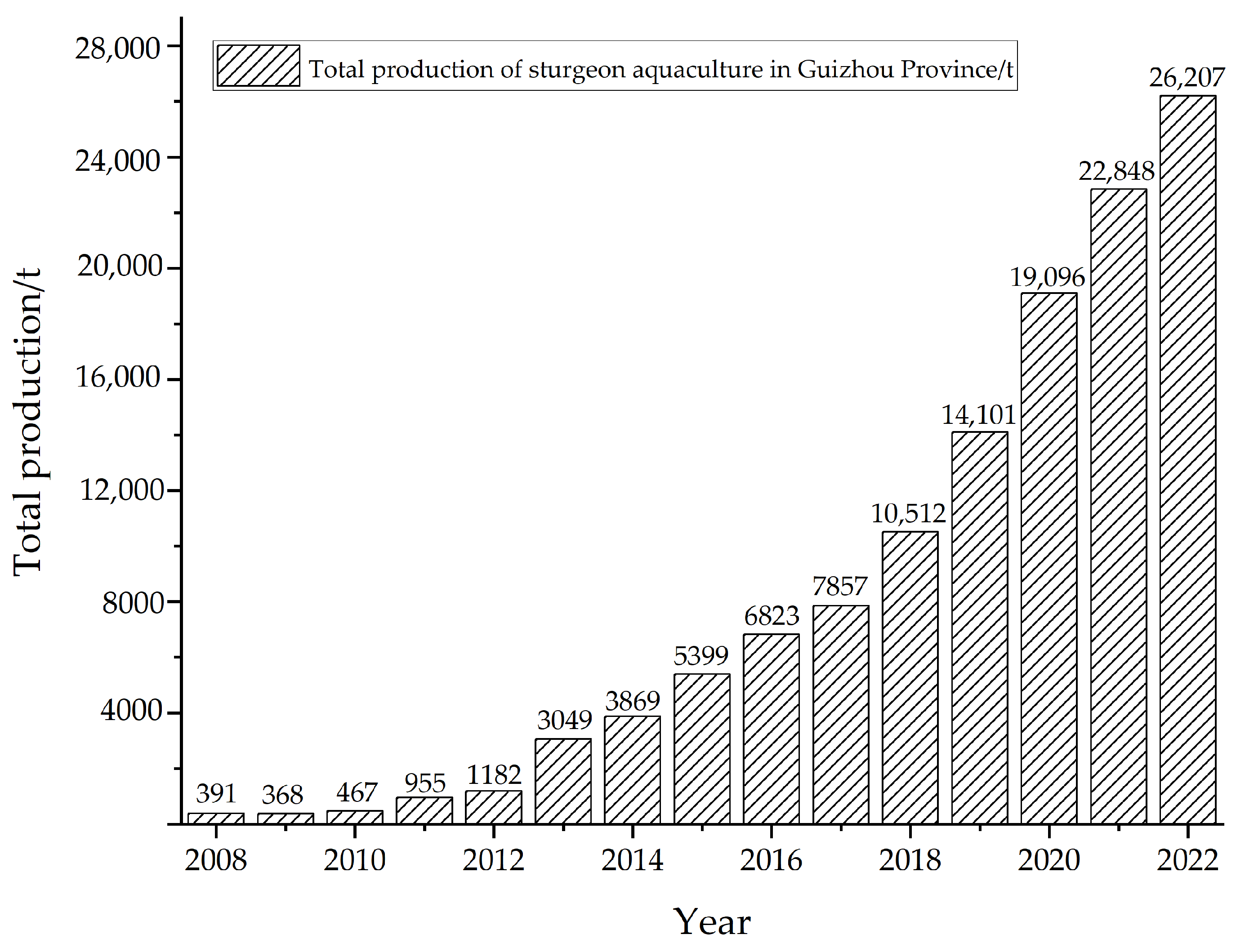
1. Introduction
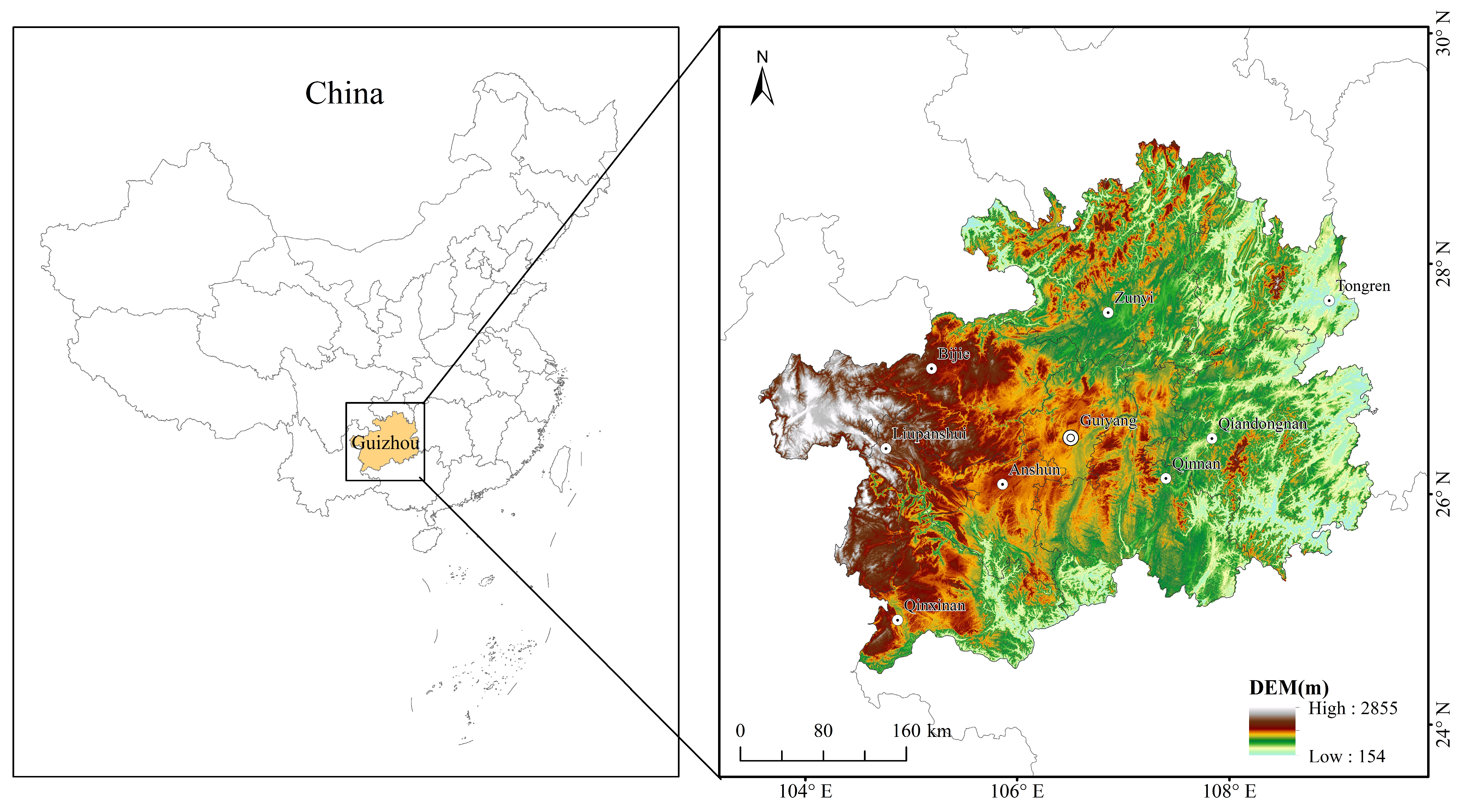
2. Study Area
3. Grey System Theory Method
3.1. The Method of Grey Prediction Analysis
3.2. The Method of Grey Correlation Analysis
4. Results
4.1. The Results of Grey Prediction Analysis
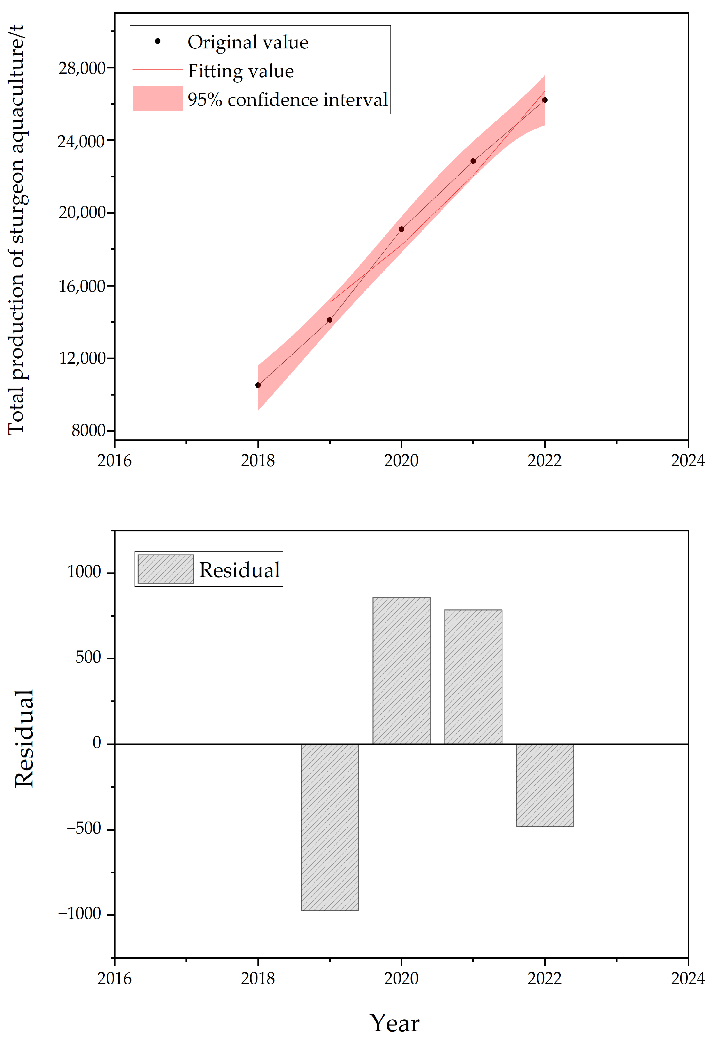
4.1.1. Modelling with Original Data from 2018 to 2022
- (1)
- Model Initialization
- (2)
- Accumulated Sequence Generation
- (3)
- Background Value Construction
- (4)
- Parameter Estimation
- (5)
- Temporal Response Formulation
- (6)
- Model Validation and Predictive Application
4.1.2. Modelling with Original Data from 2013 to 2022
- (1)
- Model Initialization
- (2)
- Accumulated Sequence Generation
- (3)
- Background Value Construction
- (4)
- Parameter Estimation
- (5)
- Temporal Response Formulation
- (6)
- Model Validation and Predictive Application
4.1.3. Modelling with Original Data from 2008 to 2022
- (1)
- Model Initialization
- (2)
- Accumulated Sequence Generation
- (3)
- Background Value Construction
- (4)
- Parameter Estimation
- (5)
- Temporal Response Formulation
- (6)
- Model Validation and Predictive Application
4.2. The Results of Grey Relational Analysis
5. Discussion
6. Conclusions
Author Contributions
Funding
Informed Consent Statement
Data Availability Statement
Conflicts of Interest
References
- Cech, J.J.; Mitchell, S.J.; Wragg, T.E. Comparative growth of juvenile white sturgeon and striped bass: Effects of temperature and hypoxia. Estuaries 1984, 7, 12–18. [Google Scholar]
- Billard, R.; Lecointre, G. Biology and conservation of sturgeon and paddlefish. Rev. Fish Biol. Fish. 2000, 10, 355–392. [Google Scholar] [CrossRef]
- Chen, H.; Hu, Q.; Kong, L.; Rong, H.; Bi, B. Effects of temperature on the growth performance, biochemical indexes and growth and development-related genes expression of juvenile hybrid sturgeon (Acipenser baerii♀ × Acipenser schrenckii♂). Water 2022, 14, 2368. [Google Scholar] [CrossRef]
- Delage, N.; Cachot, J.; Rochard, E.; Fraty, R.; Jatteau, P. Hypoxia tolerance of European sturgeon (Acipenser sturio L.; 1758) young stages at two temperatures. J. Appl. Ichthyol. 2014, 30, 1195–1202. [Google Scholar]
- Waraniak, J.; Valentine, S.; Scribner, K. Effects of changes in alternative prey densities on predation of drifting lake sturgeon larvae (Acipenser fulvescens). J. Freshw. Ecol. 2017, 32, 619–632. [Google Scholar]
- Wei, Q.W.; Zou, Y.; Li, P.; Li, L. Sturgeon aquaculture in China: Progress, strategies and prospects assessed on the basis of nation-wide surveys (2007–2009). J. Appl. Ichthyol. 2011, 27, 162–168. [Google Scholar]
- Berlinsky, D.L.; Kenter, L.W.; Reading, B.J.; Goetz, F.W. Regulating reproductive cycles for captive spawning. In Fish Physiology; Academic Press: Cambridge, MA, USA, 2020; Volume 38, pp. 1–52. [Google Scholar]
- Long, L.; Zhang, H.; Ni, Q.; Liu, H.; Wu, F.; Wang, X. Effects of stocking density on growth, stress, and immune responses of juvenile Chinese sturgeon (Acipenser sinensis) in a recirculating aquaculture system. Comp. Biochem. Physiol. C Toxicol. Pharmacol. 2019, 219, 25–34. [Google Scholar] [PubMed]
- Chen, L.; He, Z.; Gu, X.; Xu, M.; Pan, S.; Tan, H.; Yang, S. Construction of an agricultural drought monitoring model for karst with coupled climate and substratum factors—A case study of Guizhou Province, China. Water 2023, 15, 1795. [Google Scholar] [CrossRef]
- Tuo, Y.; Qiao, P.; Liu, W.; Li, Q. Predicting summer precipitation anomalies in the Yunnan–Guizhou plateau using spring sea-surface temperature anomalies. Atmosphere 2024, 15, 453. [Google Scholar] [CrossRef]
- Zhang, X.; Shang, B.; Li, X.; Li, Z.; Tao, S. Complete genome sequence data of multidrug-resistant stenotrophomonas sp. strain SXG-1. J. Glob. Antimicrob. Resist. 2020, 22, 206–209. [Google Scholar]
- Jiang, H.B.; Chen, L.Q.; Qin, J.G. Fishmeal replacement by soybean, rapeseed and cottonseed meals in hybrid sturgeon Acipenser baerii♀ × Acipenser schrenckii♂. Aquac. Nutr. 2018, 24, 1369–1377. [Google Scholar]
- Zhao, Z.; Zhao, F.; Cairang, Z.; Zhou, Z.; Du, Q.; Wang, J.; Zhang, X. Role of dietary tea polyphenols on growth performance and gut health benefits in juvenile hybrid sturgeon (Acipenser baerii♀ × A. schrenckii♂). Fish Shellfish Immunol. 2023, 139, 108911. [Google Scholar]
- Zhang, X.P.; Li, X.Y.; Yang, M.J.; Yang, X.; Zhao, F. Effect of antioxidant extracted from bamboo leaves on the quality of box-packaged sturgeon fillets stored at 4 °C. Qual. Assur. Saf. Crops Foods 2020, 12, 73–80. [Google Scholar]
- Turner, S.; Garber, P. Ripples of change: Introduced fish, ethnic minority farmers, and lively commodity chains in upland Vietnam. Hum. Ecol. 2024, 52, 797–811. [Google Scholar]
- Javanmardi, E.; Liu, S.; Xie, N. Exploring grey systems theory-based methods and applications in sustainability studies: A systematic review approach. Sustainability 2020, 12, 4437. [Google Scholar] [CrossRef]
- Nguyen, N.T.; Tran, T.T. Optimizing mathematical parameters of grey system theory: An empirical forecasting case of Vietnamese tourism. Neural Comput. Appl. 2019, 31, 1075–1089. [Google Scholar]
- Ding, S.; Li, R.; Tao, Z. A novel adaptive discrete grey model with time-varying parameters for long-term photovoltaic power generation forecasting. Energy Convers. Manag. 2021, 227, 113644. [Google Scholar]
- Chen, X.; Xie, M.; Wang, J. Gray prediction. In Application of Gray System Theory in Fishery Science; Springer: Singapore, 2023; pp. 115–163. [Google Scholar]
- Wang, Y.; Dang, Y.; Li, Y.; Liu, S. An approach to increase prediction precision of GM (1, 1) model based on optimization of the initial condition. Expert Syst. Appl. 2010, 37, 5640–5644. [Google Scholar] [CrossRef]
- Kuo, Y.; Yang, T.; Huang, G.W. The use of grey relational analysis in solving multiple attribute decision-making problems. Comput. Ind. Eng. 2008, 55, 80–93. [Google Scholar] [CrossRef]
- Liu, S.; Yang, Y.; Forrest, J.Y.L. Grey relational analysis models. In Grey Systems Analysis: Methods, Models and Applications; Springer: Singapore, 2022; pp. 77–124. [Google Scholar]
- Zhang, D.; Luo, D. Evaluation of regional agricultural drought vulnerability based on unbiased generalized grey relational closeness degree. Grey Syst. Theory Appl. 2022, 12, 839–856. [Google Scholar]
- Rehman, E.; Ikram, M.; Feng, M.T.; Rehman, S. Sectoral-based CO2 emissions of Pakistan: A novel Grey Relation Analysis (GRA) approach. Environ. Sci. Pollut. Res. 2020, 27, 29118–29129. [Google Scholar]
- Yin, J.; Cai, L.; Li, J.; Yan, X.; Zhang, B. Study on the aquaculture of large yellow croaker in the coastal zone of Zhejiang Province based on high-resolution remote sensing. Remote Sens. 2024, 17, 9. [Google Scholar] [CrossRef]
- Qazi, T.F.; Niazi, A.A.K.; Aurangzaib, A.; Mushtaq, H.; Rashid, Z.; Mojdin, H.; Jamil, A. Evaluation of Pakistan’s fisheries production as compared to other countries: A grey relational analysis. J. Soc. Signs Rev. 2024, 2, 856–884. [Google Scholar]
- Zhang, T.; Zuo, S.; Yu, B.; Zheng, K.; Chen, S.; Huang, L. Spatial patterns and controlling factors of the evolution process of karst depressions in Guizhou province, China. J. Geogr. Sci. 2023, 33, 2052–2076. [Google Scholar]
- Tan, H.; He, Z.; Yu, H.; Yang, S.; Wang, M.; Gu, X.; Xu, M. Characterization of extreme rainfall changes and response to temperature changes in Guizhou Province, China. Sci. Rep. 2024, 14, 20495. [Google Scholar]
- Fang, L.; Cong-Qiang, L.; Shi-Lu, W.; Zheng-Jie, Z. Soil temperature and moisture controls on surface fluxes and profile concentrations of greenhouse gases in karst area in central part of Guizhou Province, southwest China. Environ. Earth Sci. 2012, 67, 1431–1439. [Google Scholar]
- Zhu, D.; Xiong, K.; Xiao, H.; Gu, X. Variation characteristics of rainfall erosivity in Guizhou Province and the correlation with the El Niño Southern Oscillation. Sci. Total Environ. 2019, 691, 835–847. [Google Scholar]
- Wang, Z.; Torres, M.; Paudel, P.; Hu, L.; Yang, G.; Chu, X. Assessing the karst groundwater quality and hydrogeochemical characteristics of a prominent dolomite aquifer in Guizhou, China. Water 2020, 12, 2584. [Google Scholar] [CrossRef]
- Javed, S.A.; Liu, S. Predicting the research output/growth of selected countries: Application of Even GM (1, 1) and NDGM models. Scientometrics 2018, 115, 395–413. [Google Scholar]
- Ou, S.L. Forecasting agricultural output with an improved grey forecasting model based on the genetic algorithm. Comput. Electron. Agric. 2012, 85, 33–39. [Google Scholar] [CrossRef]
- Tsai, S.B.; Xue, Y.; Zhang, J.; Chen, Q.; Liu, Y.; Zhou, J.; Dong, W. Models for forecasting growth trends in renewable energy. Renew. Sustain. Energy Rev. 2017, 77, 1169–1178. [Google Scholar] [CrossRef]
- Bezuglov, A.; Comert, G. Short-term freeway traffic parameter prediction: Application of grey system theory models. Expert Syst. Appl. 2016, 62, 284–292. [Google Scholar]
- Xu, Y.; Wang, H.; Hui, N.L. Prediction of agricultural water consumption in 2 regions of China based on fractional-order cumulative discrete grey model. J. Math. 2021, 2021, 3023385. [Google Scholar] [CrossRef]
- Li, Q.; Sun, Y.; Liu, Z.; Ning, B.; Wu, Z. Spatial Distribution, Influencing Factors and Sustainable Development of Fishery Cultural Resources in the Yangtze River Basin. Land 2024, 13, 1205. [Google Scholar] [CrossRef]
- Su, Z.; Wu, J.; He, X.; Elumalai, V. Temporal changes of groundwater quality within the groundwater depression cone and prediction of confined groundwater salinity using Grey Markov model in Yinchuan area of northwest China. Expo. Health 2020, 12, 447–468. [Google Scholar] [CrossRef]
- Wang, Z.X.; Li, Q.; Pei, L.L. A seasonal GM (1, 1) model for forecasting the electricity consumption of the primary economic sectors. Energy 2018, 154, 522–534. [Google Scholar] [CrossRef]
- Pan, Y.; Zhang, C.C.; Lee, C.C.; Lv, S. Environmental performance evaluation of electric enterprises during a power crisis: Evidence from DEA methods and AI prediction algorithms. Energy Econ. 2024, 130, 107285. [Google Scholar] [CrossRef]
- Lyu, P.; Min, J.; Song, J. Application of machine learning algorithms for on-farm monitoring and prediction of broilers’ live weight: A quantitative study based on body weight data. Agriculture 2023, 13, 2193. [Google Scholar] [CrossRef]
- Kathirgamanathan, A.; De Rosa, M.; Mangina, E.; Finn, D.P. Data-driven predictive control for unlocking building energy flexibility: A review. Renew. Sustain. Energy Rev. 2021, 135, 110120. [Google Scholar] [CrossRef]
- Chebanov, M.; Williot, P. An assessment of the characteristics of world production of Siberian sturgeon destined to human consumption. In The Siberian Sturgeon (Acipenser baerii, Brandt, 1869) Volume 2-Farming; Springer: Cham, Switzerland, 2017; pp. 217–286. [Google Scholar]
- Edwards, P. Aquaculture environment interactions: Past, present and likely future trends. Aquaculture 2015, 447, 2–14. [Google Scholar] [CrossRef]
- Islam, M.R.; Olowe, O.S.; Mely, S.S.; Hossain, M.A.; Das, M.; Zaman, M.F.U. Review of the current situation, problems, and challenges in fish seed production and supply for Bangladesh’s aquaculture development. Aquat. Living Resour. 2023, 36, 32. [Google Scholar]
- Bostock, J.; Lane, A.; Hough, C.; Yamamoto, K. An assessment of the economic contribution of EU aquaculture production and the influence of policies for its sustainable development. Aquac. Int. 2016, 24, 699–733. [Google Scholar]
- Cai, J.; Huang, H.; Leung, P. Understanding and measuring the contribution of aquaculture and fisheries to gross domestic product (GDP). FAO Fish. Aquac. Tech. Pap. 2019, 606, 1–69. [Google Scholar]
- Valenti, W.C.; Kimpara, J.M.; Preto, B.D.L.; Moraes-Valenti, P. Indicators of sustainability to assess aquaculture systems. Ecol. Indic. 2018, 88, 402–413. [Google Scholar] [CrossRef]
- Wei, Q.; He, J.; Yang, D.; Zheng, W.; Li, L. Status of sturgeon aquaculture and sturgeon trade in China: A review based on two recent nationwide surveys. J. Appl. Ichthyol. 2004, 20, 321–332. [Google Scholar]
- Bronzi, P.; Rosenthal, H.; Gessner, J. Global sturgeon aquaculture production: An overview. J. Appl. Ichthyol. 2011, 27, 169–175. [Google Scholar]
- Oboh, A. Diversification of farmed fish species: A means to increase aquaculture production in Nigeria. Rev. Aquac. 2022, 14, 2089–2098. [Google Scholar]
- Verdegem, M.; Buschmann, A.H.; Latt, U.W.; Dalsgaard, A.J.; Lovatelli, A. The contribution of aquaculture systems to global aquaculture production. J. World Aquac. Soc. 2023, 54, 206–250. [Google Scholar]
- Zanello, G.; Fu, X.; Mohnen, P.; Ventresca, M. The creation and diffusion of innovation in developing countries: A systematic literature review. J. Econ. Surv. 2016, 30, 884–912. [Google Scholar] [CrossRef]
- Hu, F.; Zhong, H.; Wu, C.; Wang, S.; Guo, Z.; Tao, M.; Liu, S. Development of fisheries in China. Reprod. Breed. 2021, 1, 64–79. [Google Scholar]


| MAPE/% | Precision/% | Model Prediction Effect | |
|---|---|---|---|
| Grade 1 | 99 | Optimal | |
| Grade 2 | 95 | Good | |
| Grade 3 | 90 | Qualified | |
| Grade 4 | 80 | Barely qualified | |
| Above Grade 4 | Invalid |
| Year | Predicted Value/t |
|---|---|
| 2023 | 32,288.516 |
| 2024 | 39,060.662 |
| 2025 | 47,253.189 |
| 2026 | 57,164.005 |
| 2027 | 69,153.501 |
| 2028 | 83,657.656 |
| 2029 | 101,203.892 |
| 2030 | 122,430.251 |
| 2031 | 148,108.595 |
| 2032 | 179,172.678 |
| Year | Predicted Value/t |
|---|---|
| 2023 | 35,233.065 |
| 2024 | 44,343.143 |
| 2025 | 55,808.778 |
| 2026 | 70,239.039 |
| 2027 | 88,400.476 |
| 2028 | 111,257.846 |
| 2029 | 140,025.359 |
| 2030 | 176,231.176 |
| 2031 | 221,798.591 |
| 2032 | 279,148.198 |
| Year | X0 | X1 | X2 | X3 | X4 | X5 | X6 | X7 | X8 | X9 |
|---|---|---|---|---|---|---|---|---|---|---|
| 2015 | 5399 | 233,575 | 494,275.96 | 59,893 | 275,629 | 10,908.09 | 570.86 | 88.08 | 13,882 | 20,517.57 |
| 2016 | 6823 | 273,256 | 642,539.00 | 60,805 | 77,653 | 13,591.99 | 2185.25 | 70.92 | 16,416 | 19,908.43 |
| 2017 | 7857 | 241,484 | 538,291.42 | 35,177 | 74,652 | 14,015.02 | 1512.76 | 75.05 | 15,629 | 48,690.26 |
| 2018 | 10,512 | 224,172 | 474,220.70 | 47,664 | 62,417 | 11,511.37 | 1795.14 | 63.79 | 10,405 | 32,758.77 |
| 2019 | 14,101 | 227,526 | 560,606.37 | 61,532 | 74,794 | 12,282.21 | 5383.33 | 69.40 | 10,791 | 36,641.87 |
| 2020 | 19,096 | 234,673 | 606,763.88 | 64,931 | 76,354 | 10,695.31 | 7533.42 | 73.23 | 13,611 | 41,094.57 |
| 2021 | 22,848 | 250,065 | 661,370.78 | 65,679 | 73,793 | 12,332.73 | 2490.95 | 72.55 | 14,169 | 43,574.34 |
| 2022 | 26,207 | 253,933 | 775,072.32 | 67,554 | 73,415 | 12,926.38 | 3540.30 | 75.78 | 15,092 | 44,802.14 |
| Rank | Influencing Factors | Relational Degrees (R0i) |
|---|---|---|
| 1 | Aquatic seed production value, X9 | 0.8336 |
| 2 | Freshwater fishery output value, X2 | 0.8019 |
| 3 | Per capita fisher income, X5 | 0.8003 |
| 4 | Total freshwater fish production, X1 | 0.7875 |
| 5 | Fish seed quantity, X8 | 0.7828 |
| 6 | Aquaculture surface area, X3 | 0.7742 |
| 7 | Freshwater fry stock, X7 | 0.7626 |
| 8 | Technology promotion funding, X6 | 0.7199 |
| 9 | Fishery workforce, X4 | 0.7130 |
Disclaimer/Publisher’s Note: The statements, opinions and data contained in all publications are solely those of the individual author(s) and contributor(s) and not of MDPI and/or the editor(s). MDPI and/or the editor(s) disclaim responsibility for any injury to people or property resulting from any ideas, methods, instructions or products referred to in the content. |
© 2025 by the authors. Licensee MDPI, Basel, Switzerland. This article is an open access article distributed under the terms and conditions of the Creative Commons Attribution (CC BY) license (https://creativecommons.org/licenses/by/4.0/).
Share and Cite
Wang, Y.; Ni, M.; Lu, Z.; Ma, L. Prediction and Analysis of Sturgeon Aquaculture Production in Guizhou Province Based on Grey System Model. Sustainability 2025, 17, 3292. https://doi.org/10.3390/su17083292
Wang Y, Ni M, Lu Z, Ma L. Prediction and Analysis of Sturgeon Aquaculture Production in Guizhou Province Based on Grey System Model. Sustainability. 2025; 17(8):3292. https://doi.org/10.3390/su17083292
Chicago/Turabian StyleWang, Yi, Meng Ni, Zhiqiang Lu, and Li Ma. 2025. "Prediction and Analysis of Sturgeon Aquaculture Production in Guizhou Province Based on Grey System Model" Sustainability 17, no. 8: 3292. https://doi.org/10.3390/su17083292
APA StyleWang, Y., Ni, M., Lu, Z., & Ma, L. (2025). Prediction and Analysis of Sturgeon Aquaculture Production in Guizhou Province Based on Grey System Model. Sustainability, 17(8), 3292. https://doi.org/10.3390/su17083292