Article

Coupling Land Use with Multiple Geographical Factors Drives the Evolution of Habitat Quality: Case Study from Resource-Exhausted City—Jiawang District, East China

1
Institute of Geography and Tourism, Qujing Normal University, Qujing 655011, China
2
Institute for Ecological Research and Pollution Control of Plateau Lakes, School of Ecology and Environmental Science, Yunnan University, Kunming 650500, China
*
Authors to whom correspondence should be addressed.
Sustainability 2025, 17(7), 2954; https://doi.org/10.3390/su17072954
Submission received: 8 February 2025 / Revised: 12 March 2025 / Accepted: 24 March 2025 / Published: 26 March 2025

Abstract

:
Habitat quality (HQ) is crucial for assessing biodiversity and serves as a key indicator of ecosystem services and health. However, the spatial and temporal evolution of HQ under varying human activity intensities remains poorly understood. We employed the integrated valuation of ecosystem services and trade-offs model to analyze the spatiotemporal distribution and evolutionary characteristics of HQ in Jiawang District (JWD), an area experiencing resource extraction, depletion, and urban expansion. We utilized Pearson correlation analysis, partial least squares-path modeling, the generalized additive model, and patch-generating land use simulation to explore the impact of human activity on HQ and the mechanisms of multifactorial interactions. Our findings revealed the following: (1) From 2000 to 2030, HQ in JWD generally declined, with high- and low-quality areas in the north and east and the west and south, respectively. (2) The land use intensity index and population density were significantly correlated with HQ, emphasizing the role of human-driven land use changes. (3) Topographic factors were positively correlated with HQ but influenced it indirectly through land use. (4) Land use emerged as a critical intermediary influencing HQ, with climate, topography, population, and economy exerting indirect effects. These results provide insights for biodiversity conservation and sustainable urban development.

Graphical Abstract

1. Introduction

The intensifying human activity is increasingly disturbing ecosystems, diminishing the quality of biological habitats and reducing biodiversity [1]. Rapid urbanization globally, especially the extensive spread of impervious surfaces, significantly affected regional habitat quality (HQ) [2]. This problem is particularly severe in resource-depleted cities, which rely heavily on the extraction and processing of natural resources, such as coal, oil, and minerals, from which over 70% of recoverable reserves were extracted [3]. The growth of resource-exhausted cities, from the initial stages of resource exploitation to eventual depletion and subsequent economic transformation, is accompanied by intense human activities. Hence, natural habitats for wildlife are often significantly encroached upon or fragmented. This disruption substantially weakens the continuity and integrity of ecosystems, affecting the interactions and migration of species [4]. Consequently, resource-depleted cities experience significant challenges in conserving their biodiversity.
The term HQ refers to the ability of an ecosystem to provide suitable conditions for the sustainable development of individuals and populations, reflecting the status of regional biodiversity to some extent [5]. A multi-layered and complex interaction exists between resource-depleted cities and HQ. In resource-depleted cities, HQ reflects the health of the ecosystem and reveals the negative impact of prolonged resource extraction [6]. The pressure of resource depletion and economic transformation in these cities led to severe encroachment on natural habitats, such as arable land, water, and forests, and an imbalance in the urban land use structure and increasing regional landscape fragmentation [7], which seriously threatens biodiversity and human well-being [8]. Prolonged resource extraction not only alters the physical characteristics of the land but also weakens the natural restoration capacity and regulatory functions of ecosystems. For instance, a damaged ecosystem may no longer be able to effectively filter pollutants, regulate moisture, or control temperature, thereby impacting biodiversity and the ability to sustain wildlife habitats. Furthermore, a lack of funding, technology, and policies may delay environmental management and ecological restoration efforts, making it difficult to improve habitat quality. This creates a vicious cycle, exacerbating the vulnerability of ecosystems. Therefore, revealing the response of the evolution of HQ in resource-depleted cities to varying intensities of human activities and its intrinsic influence mechanism is crucial for maintaining urban biodiversity, safeguarding ecosystem stability, and promoting sustainable urban development.
Studies on HQ used several methods: (1) Evaluation method: Model simulation methods were employed for regional HQ assessments, primarily using models such as the integrated valuation of ecosystem services and trade-offs (InVEST) [9], habitat suitability index (HSI) [10], social value of ecosystem services (SoLVES) [11], and maximum entropy [12]. The InVEST model was frequently used due to its advantages of data accessibility, broad-scale applicability, low cost, high accuracy, and comprehensive framework [13]. (2) Spatiotemporal patterns: The majority of evaluations of HQ spatiotemporal changes focused on existing data from 1980 to 2020, with a minority focusing on historical and future HQ [14]. Historical and future HQ patterns were often reconstructed by backtracking or projecting land use patterns by using the InVEST model [15,16]. The evolution of future HQ patterns has significant advantages for predicting HQ trends and regional biodiversity conservation. (3) Evaluation factors: The spatial differentiation of HQ is influenced by multiple factors, including socioeconomic (e.g., gross domestic product (GDP), population density) as well as natural (e.g., temperature, precipitation) factors [17]. Researchers often examined single or dual-factor influences using methods such as ordinary least squares (OLS) [18] and geographically weighted regression (GWR) [17] for single-factor analysis or a GeoDetector [19] for dual-factor interactions. HQ evolution is driven by the interplay of multiple factors, and single- and dual-factor analyses cannot fully explain the mechanisms influencing spatial and temporal patterns.
Unlike structural equation modeling (SEM), ordinary least squares only analyzes linear relationships among explicit variables and is sensitive to multicollinearity. Geographically weighted regression focuses on the local regression analysis of geographic data but cannot manage latent variables or complex causal relationships. GeoDetectors are primarily used for qualitative analyses but do not yield quantitative results for complex causality. Partial least squares path modeling (PLS-PM) is used to manage latent variables, complex causality, covariance, and predictive power [20]; in studies requiring the integration of multiple variables and underlying structures; and to manage small samples and non-normally distributed data results, making it especially valuable under restricted data conditions. Therefore, PLS-PM has substantial advantages in research on HQ to elucidate spatial and temporal evolution mechanisms.
Furthermore, PLS-PM, a multivariate statistical analysis method, is widely used in social and management sciences and was introduced to environmental science and other fields [21]. PLS-PM, which includes non-parametric PLS-PM, combines principal component analysis and ordinary least squares regression, utilizing the advantages of regression and factor analysis to manage complex causal relationships and high-dimensional data [22]. Although PLS-PM has gradually been adopted in the environmental sciences, its potential is not fully exploited in the exploration of HQ machinery. The advent of interactive graphical interfaces enabled researchers to develop dynamic causal models more scientifically than those before its introduction due to its integrating visualization tools with PLS-PM. Another prominent advantage of PLS-PM is its ability to effectively manage multi-group issues by organizing latent and observed variables according to geographical layers such as climate, topography, and hydrology and allowing unrestricted connectivity among these groups, providing a unique approach and perspective for analyzing complex environmental problems and their response mechanisms. Few studies used the PLS-PM method to illustrate the mechanisms of HQ evolution.
Jiawang District (JWD), in the core area of the Jianghuai Ecological Economic Belt and Huaihai Economic Zone, is an important region for the South-to-North Water Transfer Project. JWD was designated as a resource-exhausted city in 2011 due to its significant ecological and environmental challenges. The damage to the natural environment due to the current methods of socioeconomic development is preventing sustainable development [23]. Thus, here, we aimed to introduce a new PLS-PM method, i.e., we used a combination of the InVEST and patch-generating land use simulation (PLUS) models to scientifically deduce the spatiotemporal pattern of future HQ. By combining PLS-PM, Pearson correlation analysis (PA), and generalized additive model (GAM), we examine the spatiotemporal evolution of HQ in JWD, investigating the impacts of human activities and the mechanisms behind the multi-factorial interactions affecting HQ. This methodological approach leverages the distinct strengths of each model, allowing for a comprehensive research framework progressing from static evaluation to dynamic forecasting and from correlation analysis to causal inference. The multi-model integration not only addresses the limitations inherent in individual methods but also enhances both the precision and predictive power of the study. Our results provide a scientific basis for protecting regional ecological diversity and ecological development.

2. Materials and Methods

2.1. Study Area

The JWD (34°17′–34°32 N, 117°17′–117°42 E), northeastern Xuzhou City, Jiangsu Province, China (Figure 1), covers an area of 612.13 km2 and includes five towns (Jiangzhuang, Qingshanquan, Zizhuang, Tashan, and Biantang), five sub-districts (Daquan, Laokuang, Pananhu, Dawu, and Damiao), and one provincial-level industrial park and lies at the interface between the low mountains and hills on the southern margin of the North China Plain and the Yellow Huaihai alluvial plain. Its topography includes low mountains, hills, piedmont plains, and alluvial plains with an elevation gradient generally higher in the west and north than in the east and south. The JWD has a warm, temperate, monsoon, semi-maritime climate characterized by distinct seasonal variations and abundant sunlight. The transportation in JWD is highly convenient, with access to highways, railways, and intercity buses. The Grand Canal and the Bulao River run across the district from east to west. The JWD region is rich in mineral resources, with 23 identified deposits, primarily coal. Due to over 130 years of coal mining, JWD was designated as one of the third batch of national resource-exhausted cities in 2011. It is a significant coal industrial base in China, having produced a total of 350 million tons of coal, making substantial contributions to the economic development of the country. However, prolonged coal mining and the growth of related industries led to severe environmental issues, creating sharp contradictions between industrial transformation, ecological restoration, and economic development. In recent years, Jiawang has actively promoted industrial transformation, leveraging ecological restoration to develop eco-tourism, smart manufacturing, modern agriculture, and trade logistics, gradually building a green economy system.

2.2. Methods

We integrated PLS-PM, PLUS models, and the PA to scientifically simulate future spatial and temporal patterns of HQ evolution and identify the mechanisms influencing HQ (Figure 2).

2.3. Data Sources

Based on the current status of the study area and relevant research [14,24], we selected 10 influencing factors from five categories: climate (i.e., annual average temperature, precipitation), topography (i.e., elevation, slope), population (i.e., population density, nighttime light index), economy (i.e., distance from the road, GDP), and land cover (i.e., land use intensity index, normalized difference vegetation index [NDVI]). To ensure a positive correlation of the factors, higher land use intensity was assigned a lower land use intensity index. The land use data are maintained at a finer resolution (30 m × 30 m) to better capture localized land cover changes that may not be well represented at coarser scales. When integrated with other datasets (1 km × 1 km), partition-based statistics are applied to calculate the characteristics of each grid cell. This ensures that land use is fully represented in the analysis without compromising spatial accuracy. The data and their sources are presented in Table 1.

2.3.1. InVEST Model Analysis

The InVEST model includes modules, such as HQ and carbon storage. Here, the HQ module of InVEST 3.13 was employed to assess the spatial and temporal changes in HQ in the JWD for the years 2000, 2010, 2020, and 2030. This module establishes the relationship between land use types and threat sources and estimates the capacity of the region to provide survival conditions for various species based on sensitivities to threat sources [25]. The HQ index ranges from 0 to 1, i.e., the higher the values, the better the HQ. Referring to existing research, we used the natural break classification method to divide the HQ index into four intervals: [0, 0.4], [0.4, 0.6], [0.6, 0.8], and [0.8, 1], defined as poor, fair, good, and excellent HQ levels, respectively. Based on an overview of the study area and existing research results, we used crops, construction, and unused land as stressors (Table 2). The sensitivity and stressor parameters were set with reference to the InVEST model manual and related research findings [15] (Table 3). The HQ index is calculated as follows:
Q x j = H x j × 1 D x j 2 D x j 2 + k 2 ,
Qxj, Hxj, Dxj, and k are the HQ of grid cell x in land use type j ranging from 0 to 1, habitat suitability of land use type j, habitat degradation index of grid cell x in land use/cover (LULC) type j, and half-saturation constant, respectively.

2.3.2. Correlation Analysis

A widely employed statistical technique for elucidating relationships between variables is PA. This technique assesses the strength of the association between two variables by computing the ratio of their covariance to the product of their standard deviations, yielding a correlation coefficient ranging from −1 to 1. This correlation coefficient is known as the Pearson correlation coefficient and is denoted as r. The formula to calculate the Pearson correlation coefficient was as follows:
R α i , α j = c o v α i , α j v a r α i × v a r α j ,
where cov, var, and ai,j are the covariance, variance, and variables, respectively.

2.3.3. PLS-PM Analysis

PLS-PM is an SEM approach designed to analyze the intricate relationships between observed and latent variables. By integrating path analysis with PLS regression techniques, PLS-PM facilitates causal and predictive analyses, including the following conditions: a small sample size, non-normal data distribution, and complex model structures [27]. It also offers distinct predictive advantages, particularly for out-of-sample predictions, and provides results more accurate than those of conventional factor analysis techniques. As a composite methodology, PLS-PM emphasizes the predictive capability and intricate relationships among explanatory variables [20]. The GoF index is frequently used in model evaluation to gauge the explanatory power of a model relative to the data.

2.3.4. GAM Analysis

Introduced by Hastie, T.J. (1990) [28], the GAM is a regression technique designed to manage nonlinear relationships between response variables and predictors. The GAM can apply linear fitting to certain explanatory variables while employing smooth function fitting for others. By assuming that each predictor is associated with a smooth, continuous, non-parametric function, the GAM models the relationship between the response variable and each predictor individually and then combines these functions additively to generate the overall prediction [29].

2.3.5. PLUS Analysis

The PLUS model is an advanced land use change simulation framework. Currently, most land use prediction models rely on cellular automata techniques, including conversion of land use and its effects at a small regional extent [30], cellular automata–Markov model [31], cellular automata–agent-based model [32], and Future Land Use Simulation model [33]. However, the cellular automata–Markov model fails to capture spatial scale variations [6]; the cellular automata–agent-based model has limitations in reflecting the effects of economic and social conditions on urban land use patterns [34]; the conversion of land use and its effects at a small regional extent model neglects non-dominant land category conversions; and it necessitates separate mathematical models for non-spatial modules [30]. The Future Land Use Simulation model struggles to capture spatial variations in land use across different regions [35]. The PLUS model addresses these limitations by employing a land expansion strategy and cellular automata with random seed variations. Here, six significant factors identified by the GAM were integrated into the PLUS model to minimize subjective influences on land use simulation, thereby enhancing the scientific rigor and accuracy of the results.
The simulation parameters for the cellular automata with multiple random seed modules in the PLUS model were configured in Table 4. A Markov chain was used to predict the demand for each land type during the accuracy verification phase for the year 2020. The settings for the neighborhood weights and land use conversion cost matrix parameters were as follows:
Neighborhood weights: These weights represent the expansion capability or conversion difficulty of different land use types, ranging from 0 to 1 (Table 5). The larger the value, the stronger the expansion capability of the land use type. The calculation formula for the neighborhood weights is as follows:
X * = X X m i n X m a x X m i n .
X * ,   X , Xmax, and Xmin represent the normalized deviation value, change in the area of each land type between the two periods of land use data, the maximum area change in all land types, and the minimum area change in all land types, respectively.
Land use conversion cost matrix: This matrix delineates the conversion rules between land types, specifying the possibility and transformation mechanisms of different land types into one another. If one land type can be transformed to another land type, the matrix entry is denoted as 1; if conversion is not possible, the matrix entry is denoted as 0. The conversion cost parameters used during the accuracy verification phase are listed in Table 6.

3. Results

3.1. Spatial and Temporal Variations in HQ

From a spatial perspective, the distribution of the HQ grades exhibited a clear pattern, with a higher quality in the eastern and northern regions than that in the western and southern regions. Most HQ grades within the study area were classified as “Fair”. Low-quality grades were primarily in Damiao Street, Laokuang Street, the Industrial Park, and the southern sections of Dahuangshan Street. High-quality grades were primarily in Pananhu Street, the southern and northern segments of Daquan Street, the Bulao River, and the Beijing–Hangzhou Grand Canal Basin (Figure 3).
Temporal analysis revealed that the average HQ indices for 2000, 2010, 2020, and 2030 were 0.260, 0.250, 0.214, and 0.217, respectively, indicating a degradation trend. The HQ within the study area was predominantly classified as “Fair” and “Poor”, with these categories collectively representing approximately 91% of the area annually. From 2000 to 2030, the proportion of “Poor”, “Fair”, “Good”, “Excellent” areas increased by 12.9%, 10.3%, and 2.6%, respectively, and remained largely unchanged, respectively. As shown in Figure 3 and Figure 4, most HQs remained stable, with quality decline concentrated in the western and southwestern regions. From 2010 to 2020, a significant increase was observed in the areas where the HQ indices had declined compared with that of the previous decade, and areas with improved indices experienced minimal change (Figure 4).
Based on land use data from 2000, 2010, and 2020, we used the PLUS model to predict the land use in JWD under a natural development scenario for the year 2030 (Figure 5). The Kappa coefficient and the overall accuracy were 0.8074 and 0.8989, respectively. This indicates that the prediction results are highly accurate and meet the precision requirements of this study. The results show that from 2000 to 2020, construction land in JWD expanded rapidly, increasing from 13.45% to 28.87%. The fragmentation of land patches intensified, while the area of grassland decreased significantly (from 5.91% to 4.53%). The area of cropland also showed a decreasing trend (from 75.24% to 75.18% and then to 61.31%), with the rate of decline initially slow and then accelerating. The area of watershed decreased first and then increased (from 3.2% to 1.67%), while woodland followed the opposite trend, first increasing and then decreasing (from 2.13% to 2.38% and then to 2.27%). Unused land also exhibited a trend of increasing and then decreasing (from 0.06% to 0.07% and then to 0.03%) (Figure 6). The spatial overlap between change areas of land use and HQ was high, indicating that HQ changed in tandem with land use. Areas of expanded construction land were often those where habitat quality declined, while areas of expanded grassland, woodland, and watershed typically saw improvements in HQ. This vividly illustrates the relationship between land use and HQ changes during different stages of development in resource-depleted cities.

3.2. Relationship Between Each Factor

PA showed that HQ was positively correlated with altitude (AL), land use intensity (LUI), slope (SL), and the NDVI and negatively correlated with the distance from roads (DisRoad), GDP, PopDen, Pre, Tem, and NL. With respect to land use, the NDVI was negatively correlated with DisRoad, GDP, LUI, PopDen, Pre, Tem, and NL and positively correlated with AL and SL. The LUI was positively correlated with AL, DisRoad, Pre, SL, and NL and negatively correlated with GDP, PopDen, and the NDVI (Figure 7).
LUI (r = 0.613, p < 0.001) and SL (r = 0.881, p < 0.001) were significantly and positively correlated with AL. DisRoad showed significant positive and negative correlations with GDP (r = 0.533, p < 0.001), NL (r = 0.497, p < 0.01), and PopDen (r = 0.401, p < 0.05) and NDVI (r = −0.722, p < 0.001), respectively. GDP was significantly positively and negatively correlated with NL (r = 0.497, p < 0.01) and NDVI (r = −0.586, p < 0.001), respectively. The LUI was significantly positively correlated with SL (r = 0.537, p < 0.001) and Pre (r = 0.361, p < 0.05). PopDen showed significant positive and negative correlations with NL (r = 0.428, p < 0.01) and Pre (r = −0.421, p < 0.05), respectively. Pre was significantly positively and negatively correlated with Tem (r = 0.920, p < 0.001) and NDVI (r = −0.344, p < 0.05), respectively. Tem was significantly negatively and positively correlated with the NDVI (r = −0.345, p < 0.05) and NL (r = 0.428, p < 0.01), respectively. The NDVI was significantly negatively correlated with NL (r = −0.545, p < 0.001) (Figure 7).

3.3. Influence Path of Factors on HQ

The PLS-PM analysis clarified the combined effects of different external factors on HQ (Figure 8). Climate had direct and indirect positive impacts on HQ (r = 0.38) and land use (r = 0.36), respectively. Terrain (r = 0.55) and economic factors (r = −0.65) did not directly affect HQ; they indirectly shaped HQ by altering land use patterns. Human activities directly and negatively impacted HQ (r = −0.54) and indirectly affected HQ by influencing land use (r = −0.55) and economic factors (r = 0.50), which vividly highlights the typical characteristics of resource-depleted cities: intense human activities are a significant driving force behind the changes in HQ.
From the perspective of factor loadings, within the population variable, NL showed the highest loading (λ = 0.99), indicating that NL was a prominent feature of population distribution, and PopDen had a smaller loading (λ = 0.57). In the economic variable, GDP exhibited the highest loading (λ = 0.90), followed by DisRoad (λ = 0.85), suggesting that GDP was the primary driver of economic activities, with DisRoad being a secondary factor with a smaller difference. Within the land use variable, the NDVI had a substantial loading (λ = 0.99), significantly higher than that of LUI (λ = 0.61), indicating that NDVI was an important reflection of land use status. For the climate variable, Pre (λ = 0.99) and Tem (λ = 0.97) showed high loadings with minimal differences, indicating an effective representation of climate characteristics. Finally, within the Terrain variable, AL (λ = 0.95) and SL (λ = 0.98) exhibited high loadings, illustrating their effective portrayal of terrain features.

3.4. Predicting the Relationship Among Variables

The GAM analysis clarified the relationships between the external factors and HQ, as highlighted in the PLS-PM results (Figure 9). Significant correlations were found between the HQ and Tem, Pre, LUI, NDVI, and PopDen. No significant correlations were found between the HQ and AL, SL, NL, GDP, or DisRoad. LUI and PopDen were positively associated with HQ, and Tem was negatively associated with HQ. Pre and NDVI exhibited a unimodal relationship with HQ.

4. Discussions

4.1. HQ Evolutionary Response to Anthropogenic Activities

The spatial distribution of the HQ within the study area exhibited clear local distinctions (Figure 3). In the southeastern region, road construction [36], industrial expansion [37], and large-scale tourism infrastructure [38] increased habitat fragmentation and disrupted ecological connectivity, reducing the HQ in several areas. In Damiao Street, Laokuang Street, the Industrial Park, and southern Dahuangshan Street, high population density [39], limited land resources [40], and intense human-land conflicts [1] associated with large-scale urbanization [18] led to further HQ decline. Contrastingly, HQ remained high on Pananhu Street and Dadong Mountain. Pananhu Street, a key area for coal mine subsidence restoration [41], benefited from abundant wetland resources and active conservation efforts, contributing to its high HQ [42]. Similarly, the Dadong Mountains area, characterized by low mountains, varied terrain, and limited human interference [43], maintained high forest cover and biodiversity. Additionally, the Bulao River and Beijing-Hangzhou Grand Canal Basin supported a high HQ, aided by ample water resources favorable to aquatic life [44]. Urbanization, industrial development, and mining activities led to a decline in HQ in the JWD region, and various natural geographical factors further contributed to the spatial differentiation of HQ (Figure 3).
The rate of change in HQ fluctuated over time, with an overall downward trend initially declining slowly and then accelerating. Between 2000 and 2020, the decline in HQ was primarily concentrated in the western and southwestern parts of the study area, likely due to rapid urbanization. As urbanization progresses, large areas of natural habitats are converted into urban construction land, disrupting the continuity and diversity of these habitats and reducing the living space for plants and animals [18]. The urbanization level in China increased from 42.99% to 54.77% in 2005 and 2014, respectively, reflecting a 27.40% increase, with the rate of urbanization peaking during this period [45]. These results indicate that urban expansion driven by rapid population growth is a significant factor influencing the evolution of HQ in the region. Prior to the implementation of the one-child policy in 1980, China experienced rapid population growth, particularly after 1949, when national policies encouraged population increase to support economic and industrial development [46]. However, this rapid population growth, coupled with the expansion of industry and agriculture, exerted immense pressure on the ecological environment [47]. The pressure on ecological space did not solely arise from population growth itself but rather from the continuous enhancement of the capacity to alter the natural environment by humanity [48].
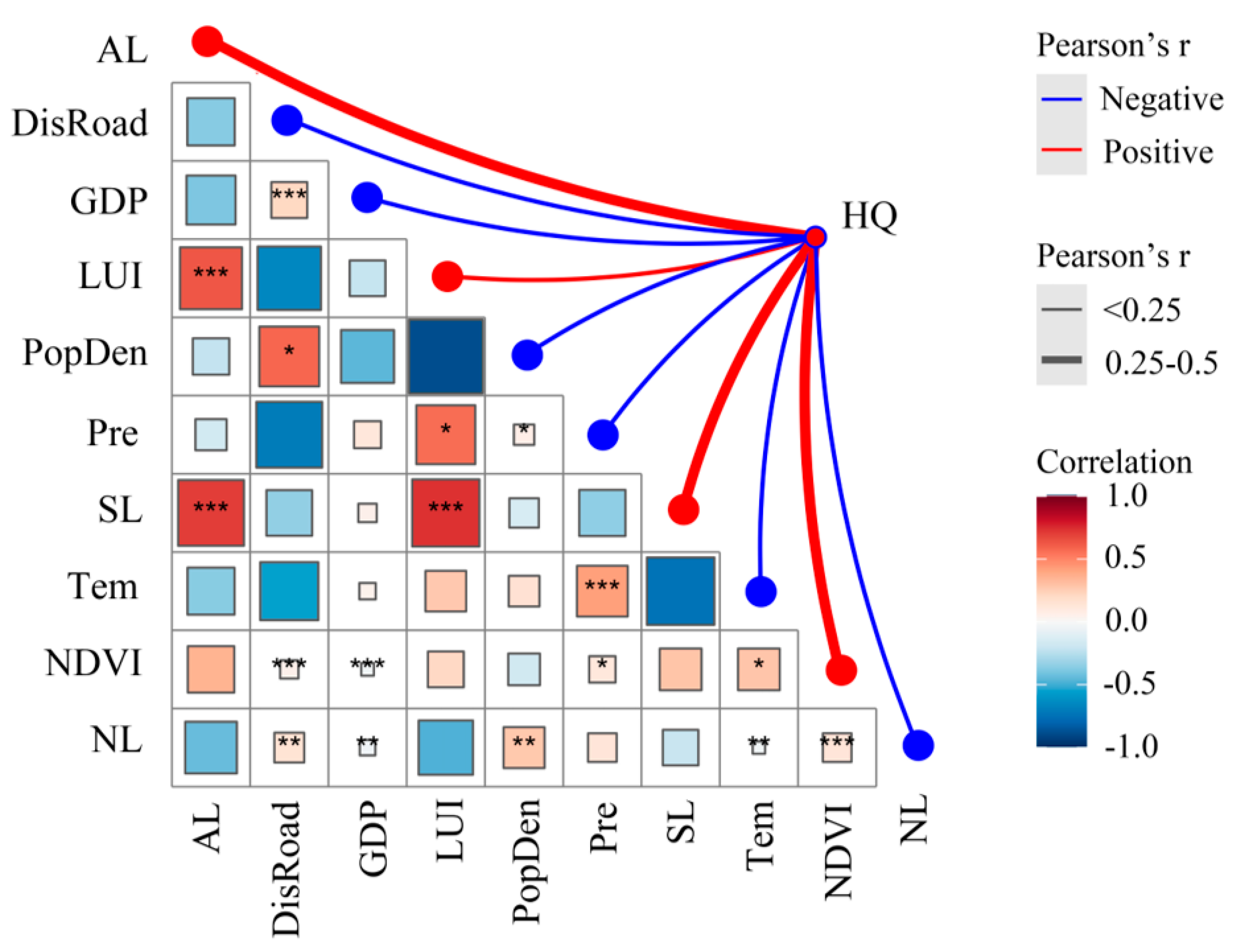
The GAM results showed a significant positive correlation between HQ and LUI and PopDen, indicating that land use and human activities were the key factors influencing HQ. This also confirms that anthropogenic activity-driven land use changes were a significant driver of the spatial and temporal evolution of HQ (Figure 8).
Specifically, from 2000 to 2010, JWD was in the expansion phase typical of resource-based cities, with rapid growth in mining areas and industrial enterprises. The resulting mining subsidence, soil pollution, and chaotic land use structure led to the creation of numerous abandoned lands. In terms of land use, this period was characterized by the expansion of construction land, a reduction in grassland, cropland, and water areas, and an increase in unused land (Figure 5). Correspondingly, the HQ also declined sharply (Figure 4).
Since being designated as a resource-depleted city in 2011, JWD has entered a transition phase. Policy shifts led to the closure of many mining areas and factories, with efforts focused on repairing mining subsidence areas, rehabilitating abandoned mines, and restoring vegetation. This transition is also marked by significant changes in land use, such as a large-scale expansion of construction land, a substantial reduction in cropland, a decrease in unused land, and an increase in woodland and water areas (Figure 5). Although urban greening and the ecological restoration of mining subsidence lands contributed to slowing down the decline in HQ [49], the rapid changes in land use under the influence of intense human activity still led to a marked decrease in HQ. For instance, large-scale tourism infrastructure projects driven by industrial transformation, such as roads and railways, often disrupt habitat integrity, resulting in fragmentation and a consequent decline in HQ [38]. Research demonstrated that land use changes significantly impact HQ. Hong et al. [50] found that the expansion of built-up areas played a key role in the degradation of regional HQ. Similarly, Kija et al. [51] attributed the decline to human activities and significant shifts in land use policies. Whittington et al. [52] showed that planned road closures significantly improved the HQ for wildlife and plants. These findings support our hypothesis that human activity is a crucial factor in the spatiotemporal evolution of HQ.

4.2. Evolutionary Trends in HQ

Under the natural development scenario, the overall HQ in the study area exhibited a slightly upward trend, although the changes were modest. In the northeastern region, habitat fragmentation decreased, leading to an improvement in the HQ from Poor to Fair. Compared with those of 2020, the proportion of Fair HQ increased significantly by 3.6% (Figure 6); the proportions of Excellent and Good HQ decreased by 0.4% and 0.6%, respectively; and the proportion of Poor HQ declined by 2.6%. This improvement was likely due to the later stage of resource-depleted city development, where government-led ecological restoration, reduced human activity, enhanced landscape connectivity [53], and the expansion of biological habitats played key roles [54]. However, in the Lake Pan’an area, HQ deteriorated from Excellent to Fair and its fragmentation increased. This decline was likely due to increased human activities, such as the expansion of construction land [51], lake reclamation [55], and tourism development [38], which contributed to the reduced HQ.
Our results revealed that the evolution of HQ in different areas was influenced by the coupled effects of various factors, including investment intensity, shifts in mining practices, population relocation policies, and urban expansion. Thus, we emphasize the importance of comprehensively coordinating resource development and utilization to maintain the functionality and stability of existing systems as much as possible, ensuring continuous improvement in HQ.

4.3. Driving Mechanisms of HQ Evolution

The results of the PLS-PM and correlation analyses (Figure 8) demonstrated that land use variables, specifically LUI and NDVI, significantly and positively impacted HQ, consistent with those of the existing research [56,57,58,59], which indicated reduced human disturbance, and a higher NDVI reflected increased vegetation coverage, both of which corresponded to improved HQ [60].
Population variables, including PopDen and NL, influenced the HQ through direct and indirect pathways. The direct impact was evidenced by a significant negative correlation between population density and HQ, with NL making the strongest contribution (λ = 0.99). This suggests that population density directly affected HQ by disrupting biological habitats through residential development [61]. According to the PLS-PM, the indirect effect of population on HQ was mediated by changes in land use patterns. Increased population density increases consumption demand and labor supply [62], attracting additional business investments and diverse economic activities. This process accelerated urbanization and increased the demand for infrastructure [63], as well as commercial and industrial land [64], leading to a decline in HQ.
Natural variables, specifically temperature and precipitation, significantly influenced HQ. Temperature and precipitation are critical determinants of HQ and directly affect survival and ecosystem functioning [65]. Variations in temperature affect soil and moisture [66], which influence microbial activity and the decomposition rate of organic matter, thereby affecting nutrient cycling and energy flow within ecosystems [67]. Precipitation regulates water availability and influences vegetation growth [68], animal hydration [69], and aquatic ecosystem health [65]. The results from the PLS-PM and GAM suggested that climatic variables indirectly affected HQ by influencing the NDVI. Optimal temperatures facilitate photosynthesis and plant growth [70], and sufficient precipitation maintains soil moisture, enhances vegetation growth and coverage [68], and increases the NDVI. Higher NDVI values generally reflect improved vegetation coverage and health, increasing areas for habitats and food resources, supporting increases in biodiversity, and enhancing ecosystem stability and resilience, thereby improving the overall HQ [71].
Additional factors, including terrain variables (AL and SL) and economic variables (GDP and DisRoad), further elucidate the complexities of HQ change mechanisms. Our findings revealed that topographical features indirectly influenced the HQ by regulating land use and vegetation cover. High altitudes and steep slopes typically experience less human disturbance than lower altitudes and slope inclines, leading to reduced LUI and increased vegetation coverage, providing more intact habitats and enhancing HQ [72,73]. Economic activities indirectly affected HQ by driving changes in land use patterns. An elevated GDP indicates increased economic activity and capital inflow, generally leading to residential construction, commercial and industrial land expansion, and infrastructure development [74]. Different stages of economic development require distinct land use types [75]; for example, the industrialization phase required extensive industrial land, and a service-oriented economy necessitated increased commercial and office spaces. Changes in industrial structure also influenced land use transformations. Proximity to major roads (i.e., DisRoad) affects land accessibility and value, shaping its specific use. Land close to major roads is more likely to develop into commercial, industrial, and high-density residential zones than land far from roads, due to the favorable transportation conditions of the former, and land far from roads is often reserved for agriculture or low-density development [76].
Here, we employed the PLS-PM approach within SEM to explore the spatial and temporal mechanisms driving HQ. SEM is a powerful statistical tool capable of identifying and analyzing complex relationships among multiple variables. The PLS-PM method, due to its strengths in managing small sample sizes and complex pathway models, was particularly well suited to our research objectives [20]. By applying PLS-PM to HQ, we quantified the effects of various variables and identified the key drivers of HQ changes along with their spatial and temporal distribution patterns. This innovative approach provides a new perspective and robust methodological foundation for understanding ecosystem changes, significantly advancing research in this field.
Research underscored the impact of land use, terrain, and economic factors on HQ; however, nonlinear interactions among these variables remain underexplored [17,77,78]. To fill this gap, we utilized a combination of PLS-PM and GAM analysis methods to elucidate the dynamic evolution of HQ and the complex interplay of the external factors influencing it; applied innovative methodologies to assess the factors affecting HQ, integrating multiple variables for a comprehensive analysis and performing a comparative evaluation; and clarified the spatiotemporal evolution of the HQ in response to varying human activity intensities.

4.4. Environment Indication and Limitation

This study introduced a novel approach for comprehensively identifying the influencing factors via multi-factor interactions and established a research paradigm specifically suited for small-scale regional studies. These findings have important implications for regional biodiversity conservation and the promotion of an ecological civilization.
We employed PLS-PM, a flexible and robust analytical tool widely used in environmental, ecological, and social sciences, to explore complex multivariate relationships. Here, PLS-PM effectively elucidated the spatial and temporal mechanisms driving the evolution of HQ and served as a reliable environmental indicator and assessment tool. Its ability to manage multicollinearity and function well with small sample sizes enhanced the robustness and reliability of the analysis. To ensure model accuracy and validity, we integrated extensive foundational data supplementing and validating the interactions among the influencing factors. This data-driven approach not only enriches the understanding of environmental change drivers but also informs the development of scientific environmental management policies.
However, despite its strengths in revealing HQ dynamics, PLS-PM has limitations. The accuracy of a model relies heavily on the quality and quantity of the underlying data; inadequate or poor-quality data can lead to inaccurate outcomes. Thus, further research should focus on improving data quality and supplementation to enhance the stability and accuracy of the model. Additionally, while PLS-PM identifies correlations between variables, its limitations in establishing causality highlight the need for future research to focus on developing standardized techniques, such as normalization or scaling, to better quantify and compare interactions among multiple influencing factors. The construction of a factor system is a crucial part of studying evolutionary mechanisms. In relatively underdeveloped fields, the establishment of a comprehensive factor system is of great significance for understanding the interactions and combinatory properties of various factors. Many of the nonlinear interactions among the variables selected here are still poorly understood. Future research should focus on the complex interactions among multiple variables to provide a deeper and more objective description of the dynamic evolution of ecological indicators. Further research should aim to verify these interactions using complementary validation methods such as experimental and long-term monitoring data. These efforts will lead to a more comprehensive and nuanced understanding of the causal relationships within complex environmental systems than those presented in this study.

5. Conclusions

We employed the InVEST, PLUS, and PLS-PM models to analyze the spatiotemporal changes in HQ in JWD and to understand the mechanisms through which various factors affect HQ. The key findings are as follows: From 2000 to 2030, the HQ in JWD exhibited a general declining trend, with high-quality areas concentrated in the east and north and low-quality areas concentrated in the west and south. The analysis revealed significant correlations between HQ, LUI, and PopDen, highlighting that changes in land use driven by human activities played a crucial role in the spatial and temporal evolution of HQ. Although topographic factors showed a significant positive correlation with HQ, they did not affect HQ directly. Instead, topography influences HQ indirectly by affecting land use patterns. Land use serves as a critical medium influencing HQ, with climate, topography, population, and economic factors indirectly affecting HQ through their effects on land use. We highlighted the complex interactions among various factors and integrated high-quality observational data using advanced mathematical models to explore the mechanisms driving changes in HQ. This is crucial for improving ecosystem stability and health, which are vital for sustainable human development.

Author Contributions

D.L. conceived the study, developed the methodology, and secured funding; M.Z. contributed to writing, reviewing, editing, formal analysis, and software; Q.L. provided supervision, software, and validation; Q.G. was responsible for data curation and formal analysis; Y.Z., Y.G., L.D., H.L. and H.Z. handled data curation, visualization, and investigation. All authors have read and agreed to the published version of the manuscript.

Funding

This research was funded by the Scientific Research Projects of the Yunnan Education Department (Grant No. 2025J0900 and 2023Y0212) and the Yunnan Fundamental Research Projects (Grant No. 202401AT070426 and 202501AU070173).

Institutional Review Board Statement

Not applicable.

Informed Consent Statement

Not applicable.

Data Availability Statement

The data and code used can be viewed online at https://doi.org/10.6084/m9.figshare.28239842.v1.

Conflicts of Interest

The authors declare no conflicts of interest.

Abbreviations

The following abbreviations are used in this manuscript:
HQhabitat quality
PLS-PMpartial least squares path modeling
GAMgeneralized additive model
PAPearson correlation analysis
PLUSpatch-generating land use simulation
InVESTintegrated valuation of ecosystem services and trade-offs
JWDJiawang District
ALaltitude
SLslope
NDVInormalized difference vegetation index
GDPgross domestic product
Preannual average precipitation
Temannual average temperature
PopDenpopulation density
NLnighttime light index
DisRoaddistance from road
LUIland use intensity

References

  1. Zhang, J.; Wang, Y.; Li, J. Maximize Eco-Economic Benefits with Minimum Land Resources Input: Evaluation and Evolution of Land Use Eco-Efficiency of Agglomerations in Middle Reaches of Yangtze River, China. Int. J. Environ. Res. Public Health 2023, 20, 1985. [Google Scholar] [CrossRef] [PubMed]
  2. Pan, Y.; Teng, T.; Wang, S.; Wang, T. Impact and mechanism of urbanization on urban green development in the Yangtze River Economic Belt. Ecol. Indic. 2024, 158, 111612. [Google Scholar] [CrossRef]
  3. Wang, J.; Li, X. Influence of industrial sustainability transition on air quality in a typical resource-exhausted city. Heliyon 2024, 10, e25138. [Google Scholar] [CrossRef]
  4. Zhuang, X.; Li, X.; Xu, Y. How Can Resource-Exhausted Cities Get Out of “The Valley of Death”? An Evaluation Index System and Obstacle Degree Analysis of Green Sustainable Development. Int. J. Environ. Res. Public Health 2022, 19, 16976. [Google Scholar] [CrossRef] [PubMed]
  5. Mallegowda, P.; Rengaian, G.; Krishnan, J.; Niphadkar, M. Assessing Habitat Quality of Forest-Corridors through NDVI Analysis in Dry Tropical Forests of South India: Implications for Conservation. Remote Sens. 2015, 7, 1619–1639. [Google Scholar] [CrossRef]
  6. Nelson, E.; Mendoza, G.; Regetz, J.; Polasky, S.; Tallis, H.; Cameron, D.; Chan, K.M.; Daily, G.C.; Goldstein, J.; Kareiva, P.M.; et al. Modeling multiple ecosystem services, biodiversity conservation, commodity production, and tradeoffs at landscape scales. Front. Ecol. Environ. 2009, 7, 4–11. [Google Scholar] [CrossRef]
  7. Li, S.; Shao, Y.; Hong, M.; Zhu, C.; Dong, B.; Li, Y.; Lin, Y.; Wang, K.; Gan, M.; Zhu, J.; et al. Impact mechanisms of urbanization processes on supply-demand matches of cultivated land multifunction in rapid urbanization areas. Habitat Int. 2023, 131, 102726. [Google Scholar] [CrossRef]
  8. Liu, H.; Zhou, L.; Tang, D. Exploring the impact of urbanization on ecological quality in the middle reaches of the Yangtze River Urban Agglomerations, China. Hum. Ecol. Risk Assess. Int. J. 2023, 29, 1276–1298. [Google Scholar] [CrossRef]
  9. Xiao, P.; Zhou, Y.; Li, M.; Xu, J. Spatiotemporal patterns of habitat quality and its topographic gradient effects of Hubei Province based on the InVEST model. Environ. Dev. Sustain. 2023, 25, 6419–6448. [Google Scholar] [CrossRef]
  10. Guan, L.; Chen, Y.; Wilson, J.A. Evaluating spatio-temporal variability in the habitat quality of Atlantic cod (Gadus morhua) in the Gulf of Maine. Fish. Oceanogr. 2017, 26, 83–96. [Google Scholar] [CrossRef]
  11. León, J.; Reijnders, V.M.J.J.; Hearne, J.W.; Ozlen, M.; Reinke, K.J. A Landscape-Scale Optimisation Model to Break the Hazardous Fuel Continuum While Maintaining Habitat Quality. Environ. Model. Assess. 2019, 24, 369–379. [Google Scholar] [CrossRef]
  12. Jeong, A.; Kim, M.; Lee, S. Analysis of Priority Conservation Areas Using Habitat Quality Models and MaxEnt Models. Animals 2024, 14, 1680. [Google Scholar] [CrossRef] [PubMed]
  13. Cao, Y.; Wang, C.; Su, Y.; Duan, H.; Wu, X.; Lu, R.; Su, Q.; Wu, Y.; Chu, Z. Study on Spatiotemporal Evolution and Driving Forces of Habitat Quality in the Basin along the Yangtze River in Anhui Province Based on InVEST Model. Land 2023, 12, 1092. [Google Scholar] [CrossRef]
  14. Zheng, H.; Li, H. Spatial–temporal evolution characteristics of land use and habitat quality in Shandong Province, China. Sci. Rep. 2022, 12, 15422. [Google Scholar] [CrossRef]
  15. Zhang, X.; Zhou, J.; LI, M. Analysis on spatial and temporal changes of regional habitat quality based on the spatial pattern reconstruction of land use. Acta Geogr. Sin. 2020, 75, 160–178. [Google Scholar] [CrossRef]
  16. Huang, Y.; Zheng, G.; Li, X.; Xiao, J.; Xu, Z.; Tian, P. Habitat quality evaluation and pattern simulation of coastal salt marsh wetlands. Sci. Total Environ. 2024, 945, 174003. [Google Scholar] [CrossRef]
  17. Fan, X.; Gu, X.; Yu, H.; Long, A.; Tiando, D.S.; Ou, S.; Li, J.; Rong, Y.; Tang, G.; Zheng, Y.; et al. The Spatial and Temporal Evolution and Drivers of Habitat Quality in the Hung River Valley. Land 2021, 10, 1369. [Google Scholar] [CrossRef]
  18. Zhu, C.; Zhang, X.; Zhou, M.; He, S.; Gan, M.; Yang, L.; Wang, K. Impacts of urbanization and landscape pattern on habitat quality using OLS and GWR models in Hangzhou, China. Ecol. Indic. 2020, 117, 106654. [Google Scholar] [CrossRef]
  19. Sun, H.; Di, Z.; Sun, P.; Wang, X.; Liu, Z.; Zhang, W. Spatiotemporal Differentiation and Its Attribution of the Ecosystem Service Trade-Off/Synergy in the Yellow River Basin. Land 2024, 13, 369. [Google Scholar] [CrossRef]
  20. McIntosh, C.N.; Edwards, J.R.; Antonakis, J. Reflections on Partial Least Squares Path Modeling. Organ. Res. Methods 2014, 17, 210–251. [Google Scholar] [CrossRef]
  21. Crocetta, C.; Antonucci, L.; Cataldo, R.; Galasso, R.; Grassia, M.G.; Lauro, C.N.; Marino, M. Higher-Order PLS-PM Approach for Different Types of Constructs. Soc. Indic. Res. 2021, 154, 725–754. [Google Scholar] [CrossRef]
  22. Schuberth, F.; Rademaker, M.E.; Henseler, J. Assessing the overall fit of composite models estimated by partial least squares path modeling. Eur. J. Mark. 2023, 57, 1678–1702. [Google Scholar] [CrossRef]
  23. Gong, X.; Chen, L.; Tan, S. Evolution of water environment construction and urban landscape ecological risk based on land cover change analysis. Water Sci. Technol. 2022, 85, 2097–2113. [Google Scholar] [CrossRef] [PubMed]
  24. Xie, B.; Zhang, M. Spatio-temporal evolution and driving forces of habitat quality in Guizhou Province. Sci. Rep. 2023, 13, 6908. [Google Scholar] [CrossRef]
  25. Leh, M.D.K.; Matlock, M.D.; Cummings, E.C.; Nalley, L.L. Quantifying and mapping multiple ecosystem services change in West Africa. Agric. Ecosyst. Environ. 2013, 165, 6–18. [Google Scholar] [CrossRef]
  26. Zhang, T.; Gao, Y.; Li, C.; Xie, Z.; Chang, Y.; Zhang, B. How Human Activity Has Changed the Regional Habitat Quality in an Eco-Economic Zone: Evidence from Poyang Lake Eco-Economic Zone, China. Int. J. Environ. Res. Public Health 2020, 17, 6253. [Google Scholar] [CrossRef]
  27. Klesel, M.; Schuberth, F.; Henseler, J.; Niehaves, B. A test for multigroup comparison using partial least squares path modeling. Internet Res. 2019, 29, 464–477. [Google Scholar] [CrossRef]
  28. Hastie, T.J. Generalized Additive Models, 1st ed.; Routledge: London, UK, 1990. [Google Scholar] [CrossRef]
  29. Ferrara, G.; Vidoli, F. Semiparametric stochastic frontier models: A generalized additive model approach. Eur. J. Oper. Res. 2017, 258, 761–777. [Google Scholar] [CrossRef]
  30. Verburg, P.H.; Soepboer, W.; Veldkamp, A.; Limpiada, R.; Espaldon, V.; Mastura, S.S.A. Modeling the Spatial Dynamics of Regional Land Use: The CLUE-S Model. Environ. Manag. 2002, 30, 391–405. [Google Scholar] [CrossRef]
  31. Ouyang, Z.; Wang, R.; Zhao, J. Ecosystem services and their economic valuation. Chin. J. Appl. Ecol. 1999, 10, 635. [Google Scholar]
  32. Li, Y.; Yao, S.; Jiang, H.; Wang, H.; Ran, Q.; Gao, X.; Ding, X.; Ge, D. Spatial-Temporal Evolution and Prediction of Carbon Storage: An Integrated Framework Based on the MOP–PLUS–InVEST Model and an Applied Case Study in Hangzhou, East China. Land 2022, 11, 2213. [Google Scholar] [CrossRef]
  33. Liu, X.; Liang, X.; Li, X.; Xu, X.; Ou, J.; Chen, Y.; Li, S.; Wang, S.; Pei, F. A future land use simulation model (FLUS) for simulating multiple land use scenarios by coupling human and natural effects. Landsc. Urban Plan. 2017, 168, 94–116. [Google Scholar] [CrossRef]
  34. Xia, M.; Zhang, Y.; Zhang, Z.; Liu, J.; Ou, W.; Zou, W. Modeling agricultural land use change in a rapid urbanizing town: Linking the decisions of government, peasant households and enterprises. Land Use Policy 2020, 90, 104266. [Google Scholar] [CrossRef]
  35. Lin, W.; Sun, Y.; Nijhuis, S.; Wang, Z. Scenario-based flood risk assessment for urbanizing deltas using future land-use simulation (FLUS): Guangzhou Metropolitan Area as a case study. Sci. Total Environ. 2020, 739, 139899. [Google Scholar] [CrossRef] [PubMed]
  36. Riedler, B.; Lang, S. A spatially explicit patch model of habitat quality, integrating spatio-structural indicators. Ecol. Indic. 2018, 94, 128–141. [Google Scholar] [CrossRef]
  37. Huo, A.; Liu, Q.; Zhao, Z.; Elbeltagi, A.; Abuarab, M.E.-S.; Ganjidoust, H. Habitat Quality Assessment and Driving Factor Analysis of Xiangyu in Feng River Basin Based on InVEST Model. Water 2023, 15, 4046. [Google Scholar] [CrossRef]
  38. Rösner, S.; Schabo, D.G.; Palme, R.; Lorenc, T.; Mussard-Forster, E.; Brandl, R.; Müller, J. High-quality habitats and refuges from tourism reduce individual stress responses in a forest specialist. Wildl. Res. 2023, 50, 1071–1084. [Google Scholar] [CrossRef]
  39. Baruah, G.; Clements, C.F.; Ozgul, A. Effect of habitat quality and phenotypic variation on abundance- and trait-based early warning signals of population collapses. Oikos 2021, 130, 850–862. [Google Scholar] [CrossRef]
  40. Carlucci, M.; Salvati, L. Assessing path-dependent urban growth with geographically weighted regressions. Environ. Impact Assess. Rev. 2023, 98, 106920. [Google Scholar] [CrossRef]
  41. Xu, J.; Yin, P.; Hu, W.; Fu, L.; Zhao, H. Assessing the ecological regime and spatial spillover effects of a reclaimed mining subsided lake: A case study of the Pan’an Lake wetland in Xuzhou. PLoS ONE 2020, 15, e0238243. [Google Scholar] [CrossRef]
  42. Rahimi, L.; Malekmohammadi, B.; Yavari, A.R. Assessing and Modeling the Impacts of Wetland Land Cover Changes on Water Provision and Habitat Quality Ecosystem Services. Nat. Resour. Res. 2020, 29, 3701–3718. [Google Scholar] [CrossRef]
  43. Yang, Z.; Liu, Y.; Su, H.; Liu, X. Exploring complex place-based coevolution of ecosystem and human activities: A case study of Qilian Mountain area in China. Int. J. Appl. Earth Obs. Geoinf. 2022, 115, 103091. [Google Scholar] [CrossRef]
  44. Shan, C.; Guo, H.; Dong, Z.; Liu, L.; Lu, D.; Hu, J.; Feng, Y. Study on the river habitat quality in Luanhe based on the eco-hydrodynamic model. Ecol. Indic. 2022, 142, 109262. [Google Scholar] [CrossRef]
  45. Zhang, X.; Song, W.; Wang, J.; Wen, B.; Yang, D.; Jiang, S.; Wu, Y. Analysis on Decoupling between Urbanization Level and Urbanization Quality in China. Sustainability 2020, 12, 6835. [Google Scholar] [CrossRef]
  46. Yuan, X.; Gao, Y. Demographic transition and economic miracles in China: An analysis based on demographic perspective. Int. J. Econ. Policy Stud. 2020, 14, 25–45. [Google Scholar] [CrossRef]
  47. Jiang, Q.; Li, S.; Feldman, M.W. China’s Population Policy at the Crossroads: Social Impacts and Prospects. Asian J. Soc. Sci. 2013, 41, 193–218. [Google Scholar] [CrossRef]
  48. Yang, L.; Xu, H.; Pan, S.; Chen, W.; Zeng, J. Identifying the impact of global human activities expansion on natural habitats. J. Clean. Prod. 2024, 434, 140247. [Google Scholar] [CrossRef]
  49. Zhao, J.; Gong, X. Animals in urban green spaces in relation to mental restorative quality. Urban For. Urban Green. 2022, 74, 127620. [Google Scholar] [CrossRef]
  50. Hong, F.; Guo, W.; Wang, H. A Comprehensive Assessment of the Hydrological Evolution and Habitat Quality of the Xiangjiang River Basin. Water 2023, 15, 3626. [Google Scholar] [CrossRef]
  51. Kija, H.K.; Ogutu, J.O.; Mangewa, L.J.; Bukombe, J.; Verones, F.; Graae, B.J.; Kideghesho, J.R.; Said, M.Y.; Nzunda, E.F. Spatio-Temporal Changes in Wildlife Habitat Quality in the Greater Serengeti Ecosystem. Sustainability 2020, 12, 2440. [Google Scholar] [CrossRef]
  52. Whittington, J.; Low, P.; Hunt, B. Temporal road closures improve habitat quality for wildlife. Sci. Rep. 2019, 9, 3772. [Google Scholar] [CrossRef] [PubMed]
  53. Jin, L.; Song, Y. Forest landscape connectivity to prioritize afforestation in urban ecosystems: Seoul as a case study. Urban For. Urban Green. 2023, 90, 128122. [Google Scholar] [CrossRef]
  54. Becker, J.A.; Hutchinson, M.C.; Potter, A.B.; Park, S.; Guyton, J.A.; Abernathy, K.; Americo, V.F.; da Conceiçāo, A.; Kartzinel, T.R.; Kuziel, L.; et al. Ecological and behavioral mechanisms of density-dependent habitat expansion in a recovering African ungulate population. Ecol. Monogr. 2021, 91, e01476. [Google Scholar] [CrossRef]
  55. Wu, Q.; Yang, R.; Yang, Z. A Study on the Rationality of Land Use Change in the Dianchi Basin during the Last 40 Years under the Background of Lake Revolution. Sustainability 2022, 14, 11479. [Google Scholar] [CrossRef]
  56. Lin, Y.; Zhang, X.; Zhu, H.; Li, R. Spatiotemporal Evolution and Mechanisms of Habitat Quality in Nature Reserve Land: A Case Study of 18 Nature Reserves in Hubei Province. Land 2024, 13, 363. [Google Scholar] [CrossRef]
  57. Wang, B.; Cheng, W. Effects of Land Use/Cover on Regional Habitat Quality under Different Geomorphic Types Based on InVEST Model. Remote Sens. 2022, 14, 1279. [Google Scholar] [CrossRef]
  58. Liao, Q.; Li, T.; Liu, D. Evolutionary patterns and influencing factors of relationships among ecosystem services in the hilly red soil region of Southern China. Environ. Monit. Assess. 2024, 196, 360. [Google Scholar] [CrossRef]
  59. Qin, X.; Yang, Q.; Wang, L. The evolution of habitat quality and its response to land use change in the coastal China, 1985–2020. Sci. Total Environ. 2024, 952, 175930. [Google Scholar] [CrossRef]
  60. Weber, D.; Schaepman-Strub, G.; Ecker, K. Predicting habitat quality of protected dry grasslands using Landsat NDVI phenology. Ecol. Indic. 2018, 91, 447–460. [Google Scholar] [CrossRef]
  61. Zhao, Y.; Qu, Z.; Zhang, Y.; Ao, Y.; Han, L.; Kang, S.; Sun, Y. Effects of human activity intensity on habitat quality based on nighttime light remote sensing: A case study of Northern Shaanxi, China. Sci. Total Environ. 2022, 851, 158037. [Google Scholar] [CrossRef]
  62. Rahman, M.M.; Saidi, K.; Mbarek, M.B. Economic growth in South Asia: The role of CO2 emissions, population density and trade openness. Heliyon 2020, 6, e03903. [Google Scholar] [CrossRef] [PubMed]
  63. Chu, C.Y.C. Population Density and Infrastructure Development. Rev. Dev. Econ. 1997, 1, 294–304. [Google Scholar] [CrossRef]
  64. Rahman, M.M.; Alam, K. Clean energy, population density, urbanization and environmental pollution nexus: Evidence from Bangladesh. Renew. Energy 2021, 172, 1063–1072. [Google Scholar] [CrossRef]
  65. Liu, J.; Ma, X.; Duan, Z.; Jiang, J.; Reichstein, M.; Jung, M. Impact of temporal precipitation variability on ecosystem productivity. Wiley Interdiscip. Rev. Water 2020, 7, e1481. [Google Scholar] [CrossRef]
  66. Jagtap, M.P.; Shinde, Y.A.; Khatri, N. An investigation on the effect of soil solarization on soil temperature and soil moisture conservation. Arab. J. Geosci. 2022, 15, 1778. [Google Scholar] [CrossRef]
  67. Li, Q.; Wang, L.; Fu, Y.; Lin, D.; Hou, M.; Li, X.; Hu, D.; Wang, Z. Transformation of soil organic matter subjected to environmental disturbance and preservation of organic matter bound to soil minerals: A review. J. Soils Sediments 2023, 23, 1485–1500. [Google Scholar] [CrossRef]
  68. Harris, B.L.; Taylor, C.M.; Weedon, G.P.; Talib, J.; Dorigo, W.; van der Schalie, R. Satellite-Observed Vegetation Responses to Intraseasonal Precipitation Variability. Geophys. Res. Lett. 2022, 49, e2022GL099635. [Google Scholar] [CrossRef]
  69. Grinath, J.B.; Deguines, N.; Chesnut, J.W.; Prugh, L.R.; Brashares, J.S.; Suding, K.N. Animals alter precipitation legacies: Trophic and ecosystem engineering effects on plant community temporal dynamics. J. Ecol. 2018, 106, 1454–1469. [Google Scholar] [CrossRef]
  70. Zhang, P.; Kuramae, A.; van Leeuwen, C.H.A.; Velthuis, M.; van Donk, E.; Xu, J.; Bakker, E.S. Interactive Effects of Rising Temperature and Nutrient Enrichment on Aquatic Plant Growth, Stoichiometry, and Palatability. Front. Plant Sci. 2020, 11, 58. [Google Scholar] [CrossRef]
  71. Hernández, M.; Borges, A.A.; Francisco-Bethencourt, D. Mapping stressed wheat plants by soil aluminum effect using C-band SAR images: Implications for plant growth and grain quality. Precis. Agric. 2022, 23, 1072–1092. [Google Scholar] [CrossRef]
  72. Chen, S.; Ma, M.; Wu, S.; Tang, Q.; Wen, Z. Topography intensifies variations in the effect of human activities on forest NPP across altitude and slope gradients. Environ. Dev. 2023, 45, 100826. [Google Scholar] [CrossRef]
  73. Wu, Y.; Wang, J.; Gou, A. Research on the evolution characteristics, driving mechanisms and multi-scenario simulation of habitat quality in the Guangdong-Hong Kong-Macao Greater Bay based on multi-model coupling. Sci. Total Environ. 2024, 924, 171263. [Google Scholar] [CrossRef] [PubMed]
  74. Wu, J.; Luo, J.; Zhang, H.; Qin, S.; Yu, M. Projections of land use change and habitat quality assessment by coupling climate change and development patterns. Sci. Total Environ. 2022, 847, 157491. [Google Scholar] [CrossRef] [PubMed]
  75. Burtle, J. Parametric Maps of Different Types of Economic Development. Rev. Econ. Stat. 1960, 42, 44–55. [Google Scholar] [CrossRef]
  76. Ng, C.P.; Law, T.H.; Wong, S.V.; Kulanthayan, S. Relative improvements in road mobility as compared to improvements in road accessibility and economic growth: A cross-country analysis. Transp. Policy 2017, 60, 24–33. [Google Scholar] [CrossRef]
  77. Cui, G.; Zhang, Y.; Shi, F.; Jia, W.; Pan, B.; Han, C.; Liu, Z.; Li, M.; Zhou, H. Study of Spatiotemporal Changes and Driving Factors of Habitat Quality: A Case Study of the Agro-Pastoral Ecotone in Northern Shaanxi, China. Sustainability 2022, 14, 5141. [Google Scholar] [CrossRef]
  78. Dalu, T.; Mwedzi, T.; Wasserman, R.J.; Madzivanzira, T.C.; Nhiwatiwa, T.; Cuthbert, R.N. Land use effects on water quality, habitat, and macroinvertebrate and diatom communities in African highland streams. Sci. Total Environ. 2022, 846, 157346. [Google Scholar] [CrossRef]
Figure 1. Location of Jiawang District. (a) Provincial boundaries of China, (b) municipal boundaries of Jiangsu, and (c) county-level boundaries of Xuzhou. Additionally, (d) elevation map of Jiawang District, while (e) land use distribution within the district.
Sustainability 17 02954 g001
Figure 2. Technical roadmap of this study. Pre = average annual precipitation, Tem = average annual temperature, AL = altitude, SL = slope, NDVI = normalized difference vegetation index, PopDen = population density, NL = night light index, DisRoad = distance from the road, LUI = land use intensity index, GDP = gross domestic product, PA = pearson correlation coefficient, PLS-PM = partial least squares path modeling, GAM = generalized additive model.
Sustainability 17 02954 g002
Figure 3. Spatiotemporal distribution of HQ from 2000 to 2030.
Sustainability 17 02954 g003
Figure 4. Stacked percentage bar chart of HQ from 2000 to 2030.
Sustainability 17 02954 g004
Figure 5. Spatiotemporal distribution of land use from 2000 to 2030.
Sustainability 17 02954 g005aSustainability 17 02954 g005b
Figure 6. Stacked percentage bar chart of land use from 2000 to 2030.
Sustainability 17 02954 g006
Figure 7. Correlation between impact factors. Red and blue lines indicate significant positive and negative correlations, respectively. Stars in the lower left corner indicate significant correlations. (* p < 0.05, ** p < 0.01, *** p < 0.001). AL = altitude, SL = slope, NDVI = normalized difference vegetation index, NL = night light index, DisRoad = distance from the road, GDP = gross domestic product, Pre = average annual precipitation, Tem = average annual temperature, PopDen = population density, LUI = land use intensity index.
Sustainability 17 02954 g007
Figure 8. PLS-PM illustrating the direct and indirect effects of climate, topography, land use, population, and economic factors on HQ (goodness of fit = 0.531). Solid and dashed lines denote significant (* p < 0.05, ** p < 0.01, *** p < 0.001) and non-significant paths, respectively. Orange and blue lines denote positive and negative correlations, respectively. Line thickness corresponds with correlation strength. Coefficients on orange and blue lines represent correlation coefficients; numbers on the black lines represent loadings of indicators on latent variables. AL = altitude, SL = slope, NDVI = normalized difference vegetation index, NL = night light index, DisRoad = distance from the road, GDP = gross domestic product, Pre = average annual precipitation, Tem = average annual temperature, PopDen = population density, LUI = land use intensity index.
Sustainability 17 02954 g008
Figure 9. Relationship between influencing factors and HQ based on the GAM. Non-significant fitting lines are represented as dashed lines. (a) Predicted relationship between Tem and HQ. (b) Connection between Pre and HQ. (c) Association between AL and HQ. (d) Linkage between SL and HQ. (e) Correlation between LUI and HQ. (f) Relationship between NDVI and HQ. (g) Interaction between PopDen and HQ. (h) Relationship between NL and HQ. (i) Connection between GDP and HQ. (j) Association between DisRoad and HQ.
Sustainability 17 02954 g009
Table 1. Used data and their sources. Annual average temperature and precipitation reflect regional climate, influencing ecosystems and human activities. NDVI measures vegetation coverage, while land use data (2000, 2010, 2020) and intensity track human impact on land. Administrative boundaries define jurisdictional areas, and population density indicates settlement patterns. Nighttime light index serves as a proxy for economic activity, while GDP quantifies economic output. Elevation and slope shape landforms and land use suitability. Distance from the road affects accessibility and development potential.
DataSources
Annual average temperatureData Center for Resources and Environmental Sciences of the Chinese Academy of Sciences (http://www.resdc.cn) and calculated using ArcGIS, land use resolution is 30 m × 30 m, others are 1 km × 1 km
Annual average precipitation
Normalized difference vegetation index
Administrative boundaries
Population density
Nighttime light index
Land use intensity
Land use for 2000, 2010, and 2020
Gross domestic product
ElevationGeospatial Data Cloud (http://www.gscloud.cn/) and calculated using ArcGIS
Slope
Distance from the roadOpen Street Map (http://www.openstreetmap.org/) and calculated in ArcGIS
Table 2. Threat source and its maximum impact distance, threat source weight, and recession type.
Threats FactorMax Distance of Influence (km)WeightsDecay Type
Cropland4.00.6Linear
Construction land8.00.4Exponential
Unused land6.00.5Linear
Table 3. Habitat suitability and land use type sensitivity to each threat factor [26].
Land Use TypesHabitat SuitabilityCroplandConstruction LandUnused Land
Cropland0.30.00.80.4
Woodland1.00.60.40.2
Grassland1.00.80.60.6
Watershed0.70.50.40.2
Construction land0.00.00.00.1
Unused land0.60.60.40.0
Table 4. Parameter setting for cellular automata simulation.
Patch Generation ThresholdExpansion CoefficientPercentage of Seeds
0.50.30.02
Table 5. Domain weight setting.
Land CoverCroplandWoodlandGrasslandWatershedConstruction LandUnused Land
Domain weighting0.7390.0420.2820.0630.9990.001
Table 6. Cost matrix setup for land use conversion.
Land CoverCroplandWoodlandGrasslandWatershedConstruction LandUnused Land
Cropland111111
Woodland111011
Grassland111111
Construction land111011
Unused land111111
Disclaimer/Publisher’s Note: The statements, opinions and data contained in all publications are solely those of the individual author(s) and contributor(s) and not of MDPI and/or the editor(s). MDPI and/or the editor(s) disclaim responsibility for any injury to people or property resulting from any ideas, methods, instructions or products referred to in the content.

