Critical Analysis of the Results of a Network System for Nitrogen Dioxide Monitoring

Abstract

Data relative to the nitrogen dioxide concentrations of seventeen fixed monitoring stations in three provinces in Po Valley in Northern Italy are analysed. NO₂ is considered to be one of the most harmful air pollutants, mainly due to vehicle traffic in urban environments. According to the EU directives, different categories of monitoring sites are identified as being representative of different situations. The main objective of this study was to check the agreement of the classification of monitoring sites with the chemical measurements of the actual atmospheric NO₂ pollution. The analysis considered the whole year of 2022 and even included the consideration of single months; the aim was to identify seasonal effects. The data were treated using different chemometric techniques, and the results obtained from significance tests were consistent with those of cluster analyses. In particular, both approaches to the treatment of the chemical data indicate that the level of NO₂ pollution may be significantly different from one station to another, even within the same category, and may produce results that are more similar to those of different categories, both inside the same province and in different provinces. Beyond local interest, this work also acts as a case study, attempting to offer a path for a common approach to effective reproducible monitoring procedures toward shared environmental sustainability.

1. Introduction

Air pollution should be considered as a priority with respect to human health, since it may be the cause of cardiovascular and respiratory diseases and even of premature death [1,2]. Prevention, control, and interventions to mitigate such a threat to both present and future generations constitute an urgent need, in the topical frame of sustainability, for more and more invasive anthropic actions. Each of the listed steps requires the carefully performed monitoring of the evolving situations, by properly choosing locations where environmental controls can be activated, even exploiting the ascertained seasonal dependence of atmospheric pollution [3].

On the one hand, the sensing systems that are currently available seem suitable for the execution of effective analytical procedures. However, adequate attention has not always been paid to ensure the best location of monitoring sites that are suitable for drawing a spatial map that is representative of pollution levels. Time mapping, including the identification of significant seasonal variations, is equally important and, although limited to the monitored sites, is possible; statistically valid conclusions can be drawn once a proper treatment of the collected data is performed.

Chemometric techniques, namely significance tests and classification or pattern recognition procedures, constitute the mandatory tools for this purpose; these are only adequate to provide a picture of the situation on the basis of the active monitoring network [4]. In addition, to allow for the acquisition of information about where, when, and how to act in the mitigation process, as a function of the nature of the pollutants identified, the obtained results are even suitable for proposing improvements to the structure of the network itself. In fact, the sustainability of the spatially and temporally evolving anthropic pressures requires continuous control and an upgrade to the monitoring networks in order to adapt the interventions to dynamic situations [3].

It should be evidenced that the percentage of the EU urban population exposed to air pollutant concentrations above those fixed by the World Health Organization (WHO) guidelines was estimated at 88% for NO₂, 94% for O₃, and 96% for PM_2.5 in the year 2022 [1]. Although the concentration of most pollutants in the air has decreased since 2000, the most recent report published by the European Environment Agency (EEA) in 2023, which was updated in 2024, underlines that the health risks, including the premature deaths, caused by long-term exposure to particulate matter and NO₂ are still shockingly high [2].

In order to reduce the concentrations of the most important air pollutants, the member states of the European Union (EU) are required to present air quality plans, mainly focusing on reducing NO₂, PM₁₀, and PM_2.5 emissions through the activation of specific actions to reduce the pollutant exceedances and improve air quality. In particular, NO₂ is responsible for serious adverse effects on health, such as cardiovascular diseases [5]; the causal relationship between long-term exposure to NO₂ and respiratory effects has also been assessed [6]. EU regulatory limits for NO₂ establish an hourly average maximum (200 μg/m³, which is not to be exceeded more than 18 times per year) and an annual average maximum (40 μg/m³). The recently issued European Directive concerning air quality—EU 2024/2881—pursues the aim of achieving a zero-pollution objective by 2050 through the revision of current EU regulatory limits of air pollutant levels, in accordance with the most recent scientific evidence. In fact, the WHO guidelines, as revised in 2021 [7], are more restrictive than EU regulatory standards. As concerns NO₂, whereas the hourly average limit in EU 2024/2881 remains fixed at 200 μg/m³, which is not to be exceeded more than three times a year, the target annual average value is 20 μg/m³, which is to be reached, through several interim targets, by 2030 (the first interim target is set at 40 μg/m³). A further short-term recommended value has been introduced, i.e., a daily average value of 50 μg/m³.

In anthropised areas, combustion processes constitute the main source of NOx, namely NO and NO₂. A major contribution is ascribed to road transport; industrial combustion processes and energy supply [1] are other important sources. Among the NOx species, which are precursors of tropospheric ozone, particulate matter, and rain acidification, attention is mainly devoted to NO₂; this is the only nitrogen oxide regulated by the EU directive because of its high toxicity. The exceedances of NO₂ levels with respect to EU air quality standards are ascribed to road traffic in urban centres in many countries [8], including Italy [9,10].

In addition to the cited primary origin, secondary NO₂ is formed by the oxidation of NO, which proceeds through complex reactions involving volatile organic compounds (VOCs), O₃, and CO. On the other hand, NO₂ is a relatively short-lived species, undergoing photodissociation, followed by the formation of ozone; this is characterised by various toxic effects. The estimated NO₂ lifetime ranges from about 2 to 8 h, depending on latitude and meteorological conditions [11,12]; this results in reduced spatial diffusion. Studies performed on near-road pollution sources reveal that the NO₂ produced by motor vehicles progressively lowers to the background concentration at a distance of 550 m from the road edge [13].

A peculiar period with respect to emissions from vehicle traffic is represented by the lockdown during the COVID-19 pandemic in 2020; the concentrations of pollutants in the air in 2020 and 2021, i.e., during and just after the timeframe affected by the restrictions on working and social activities, were analysed in many scientific articles [14,15,16,17,18,19]. All studies led to the conclusion that a meaningful lowering of the level of pollutants in the air occurred in 2020 and 2021, especially that of NO₂. This is the reason why we decided to analyse data relative to 2022, which seems to constitute, quite reasonably, a time that is suitable to stop the movie and to take a picture of the situation; in fact, we are supposed to be in a quasi-steady-state condition. We hope that 2022, at least limited to countries that most convincingly claim to be involved in sustainability transitions, may also be considered as the starting year with respect to such a process. Hence, it may constitute a reference for future analyses, deserving specific attention.

In particular, NO₂ constitutes an excellent indicator, both in temporal and in spatial frames, of air pollution due to vehicle traffic, specifically when the relevant data collected close to the road are compared with those far enough from the source [20]. For a number of reasons, there is an urgent need to arrange spatial maps of the concentration levels of NO₂ and to follow similar maps over time. Fixed monitoring stations operate all over the EU that are devoted to quantifying the amount of a set of air pollutants in a quasi-continuous way.

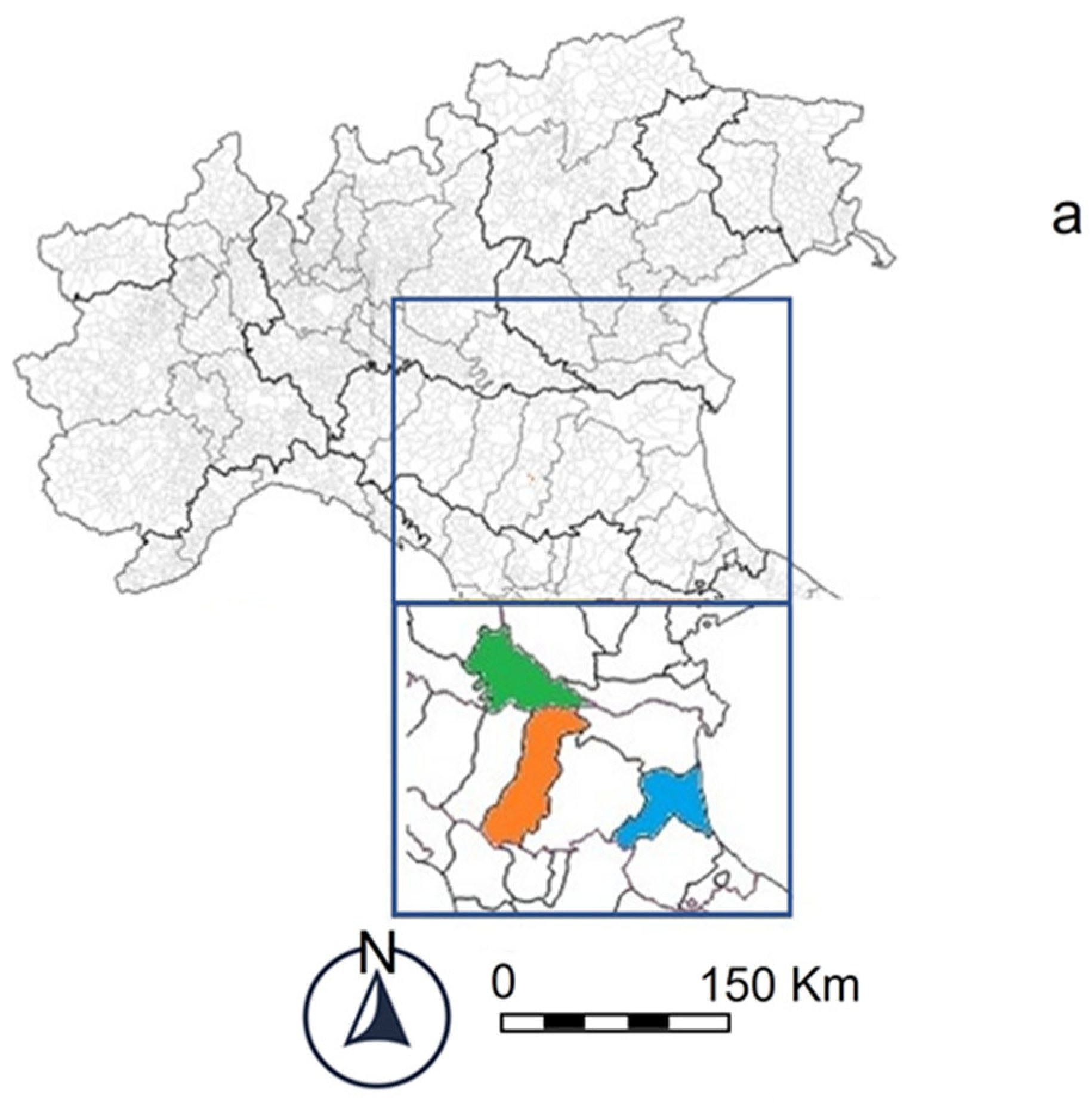
The area we chose for this study is located in the Po Valley, which constitutes a peculiar case in terms of atmospheric pollution. This area, located in Northern Italy, is acknowledged as one that is suffering the worst air quality in western Europe [21], mainly in relation to PM₁₀, PM_2.5, O₃, and NO₂. Such evidence is the consequence of the combination of three main negative factors: (i) intense industrial activity; (ii) high population density; and (iii) meteorological conditions. A high traffic volume constitutes a direct consequence. The Po Valley is often under high-pressure atmospheric and thermal inversion conditions. In the cold months, fog and low clouds block air pollutants, and the mountains surrounding the valley strongly limit the air circulation, making conditions unfavourable to the dispersion of pollutants.

In order to provide an account of a specific, heavy situation, data relative to the air pollution collected in 17 monitoring stations differently located within the area of the provinces of Modena, Mantova, and Ravenna, located in the Po Valley, Italy, were considered.

Hourly data of NO₂ concentrations are available from the websites of the institutions to which the stations refer. Box plots complement the data files published [22], by offering a visualisation of the situation in the different monitoring stations all year long, as well as day by day, in the different months of the year. In these reports, general statistics of concentration data in the specific period analysed, as well as exceedances of the air quality EU limits, are reported.

Based on the huge amount of collected data, it was deemed appropriate to perform a deeper treatment of the data, not only to report them in a concise form, but also to allow for an effective and meaningful comparison between the NO₂ detection data in sites planned to detect similar or different situations, as well as in different seasons, in order to offer effective scientific support to subsequent intervention actions. The locations of the stations, intentionally devoted to providing an exhaustive picture of NO₂ pollution in the areas, were critically analysed and discussed.

This study may possibly allow for considerations and conclusions to be drawn beyond the peculiar geographic location of the monitoring stations considered, suggesting a few general key points as regards the following: (i) the highest importance should be ascribed to the chemical data when fixing the criteria on which the locations of the stations are based; (ii) the possibility to draw a space–time map on which conclusions should be drawn out, carefully considering both the peculiarity of some situations and the seasonal character of the sources of NO₂ pollution; and (iii) the offer of a possible effective and reproducible treatment of data that, in turn, allows for comparisons and shareable criteria for the identification of different typologies of environment in which the stations are located. Suggestions of consequent possible interventions to mitigate pollution phenomena may constitute the spontaneous consequence.

Suitable and robust statistical tools were adopted in order to ascribe statistical significance to the results and to make the data widely accessible to those whose subsequent actions are required. Notice that, as described in the NO₂ Data Analysis section, we adopted chemometric techniques that are most widely diffused, and are, consequently, well known in the ‘world’ of analytical and environmental chemists; they are easily accessible through user-friendly software packages using data sheets for input. The choice was made aiming to enable the easy reading, exchange, and comparison of results obtained through widely diffused statistical instruments. Here, a fundamental step of the monitoring pipeline should be emphasised, which may also suggest suitable changes in the preceding phases, allowing for a comparison of data collected in different situations; this consists of drawing a common and easily accessible path for the critical analysis of the data from a statistical point of view. The goal of the present article is to provide a contribution to this field of study.

2. Materials and Methods

2.1. Air Quality Monitoring Network

According to the European Directives, air quality monitoring is based on a network of stations located in zones and agglomerations in each member state. The information on air quality obtained in this way should be comparable across the European Union. Although monitoring points suffer from a limited distribution, allowing for doubts about their effective spatial representativeness [23], they still constitute reference sites, providing accurate measurements of ground-level air pollutant concentrations. On the other hand, the wide spatial coverage of satellite observations furnishes data relative to the NO₂ tropospheric column density, which cannot act as a substitute for the monitoring points located on the ground, although many studies have attempted a correlation between the two measurements [24].

The locations of currently operating fixed stations are chosen on the basis of the criteria established by Directive 2008/50/CE and the Italian D.Lgs 155/2010, i.e., (i) dominant emissive sources, indicated as traffic, industrial, and background stations; (ii) location with respect to the distribution and density of residential buildings, indicating the relevant stations as urban, suburban, and rural. The concentrations of pollutants in urban background sites are not affected by a single emissive source, and the relevant data aim to be representative of the average background exposure of the population. On the other hand, the urban traffic sites, located in close proximity to major roads, represent urban environments that are more severely polluted by traffic. It is evident that urban locations, typically chosen to be well inside the urban pattern, are also affected in the winter season by combustion pollution from private houses and offices.

Since this study utilises data from monitoring stations in Italy, it seems appropriate to expose a few guidelines that are specifically adopted in this country. According to D.Lgs 155/2010, i.e., the Italian transposition of Directive 2008/50/CE, the agglomerations and zones, as well as the location of monitoring stations, are identified by the regional authority; the Region Institution is in charge of managing the monitoring station network through a regional agency for environment protection, called Agenzia Regionale per la Protezione Ambientale (ARPA). It should be underlined that the criteria adopted by the local agencies follow those adopted at the European level, adapting them to the specific situations of the relevant territory. In all the selected stations, monitoring is operated by automated analysers. The reference method for the measurements of the concentrations of NO₂ and NO, according to the European Directive, is based on chemiluminescence, according to UNI EN 14211:2005 (https://store.uni.com/uni-en-14211-2005; accessed on 11 January 2025). An established quality control system and quality assurance system are adopted by the ARPA operators.

We analysed the day-by-day hourly concentration data of NO₂ collected in 2022 in three provinces of the Po Valley—Modena, Mantova, and Ravenna. The province of Modena extends from the Appennini mountains to the centre of the Po Valley; it should be noted that the monitoring stations are located in the flat portion of the province, at an altitude from 20 to 115 m above sea level. The province of Mantova borders with the province of Modena; it is almost completely flat and extends above sea level from 5 to 200 m altitude in the central part of the Po Valley. The province of Ravenna (from 10 to 220 metres above sea level) is located in the eastern portion of the Po Valley, adjacent to the Adriatic Sea. The number of inhabitants living in these provinces is 708,600, 407,000, and 389,000, respectively, and the corresponding population density is 264, 174, and 209 inhabitants/Km². Modena and Ravenna belong to the same region—Emilia-Romagna—but are affected by different meteorological conditions, as can easily be inferred from the notably different distance from the sea. Mantova is similar to Modena as concerns meteorological conditions, belonging to the Lombardia region. The considered area is highly anthropised, as is testified in the reported data; furthermore, many industrial sites and intensive agricultural cultivations are present.

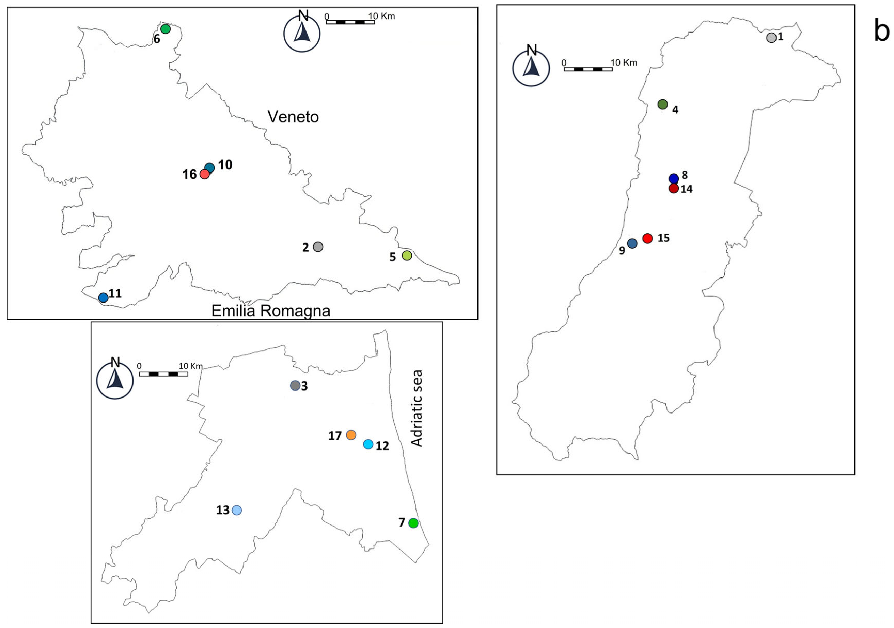
Four categories of stations are identified, labelled as urban traffic (UT), urban background (UB), suburban background (SB), and rural background (RB), respectively. Six of the chosen seventeen stations devoted to air quality monitoring are located in the province of Modena, six are in the province of Ravenna, and five are in the province of Mantova. A map representing the area is shown in Figure 1. The locations and categories accounting for the classification of the seventeen stations are reported in

Table 1. Province, denomination assigned by ARPA, and categories of the air quality monitoring stations. In the last two columns, the relevant abbreviations and ID numbers used throughout the article are reported. UT stands for urban traffic, SB for suburban background, UB for urban background, RB for rural background; Mo, Mn, and Ra stand for Modena, Mantova, and Ravenna, respectively; the final number in the abbreviation indicates different stations in the same province, within the same category.

Province	Station	Category	Abbreviation	ID
Modena (MO)	Modena-Giardini	UT	UT-Mo1	14
Modena (MO)	Fiorano Modenese-San Francesco	UT	UT-Mo2	15
Modena (MO)	Modena-Parco Ferrari	UB	UB-Mo1	8
Modena (MO)	Sassuolo-Parco Edilcarani	UB	UB-Mo2	9
Modena (MO)	Carpi-Remesina	SB	SB-Mo	4
Modena (MO)	Mirandola-Gavello	RB	RB-Mo	1
Mantova (MN)	Mantova-Gramsci	UT	UT-Mn	16
Mantova (MN)	Mantova-S. Agnese	UB	UB-Mn1	10
Mantova (MN)	Viadana	UB	UB-Mn2	11
Mantova (MN)	Sermide	SB	SB-Mn1	5
Mantova (MN)	Ponti sul Mincio	SB	SB-Mn2	6
Mantova (MN)	Schivenoglia	RB	RB-Mn	2
Ravenna (RA)	Ravenna-Zalamella	UT	UT-Ra	17
Ravenna (RA)	Ravenna-Caorle	UB	UB-Ra1	12
Ravenna (RA)	Faenza-Parco Bertozzi	UB	UB-Ra2	13
Ravenna (RA)	Cervia-Delta Cervia	SB	SB-Ra	7
Ravenna (RA)	Alfonsine-Ballirana	RB	RB-Ra	3

. Stations classified as industrial were not considered, because they are influenced by peculiar emissive sources.

2.2. NO₂ Data Analysis

NO₂ concentration data were obtained from the archives of the website of the ARPA of Regione Emilia-Romagna (https://dati.arpae.it/dataset/qualita-dell-aria-rete-di-monitoraggio/resource/70da49ad-46d6-4945-90ee-4149016a40bf; accessed on 11 January 2025) or were requested from the ARPA of Regione Lombardia (https://www.arpalombardia.it/temi-ambientali/aria/form-richiesta-dati-stazioni-fisse; accessed on 11 January 2025). The hourly concentration values of NO₂ reported in the available data are obtained, according to the analytical methodology indicated by the EU community legislation, by monitoring measurements and reporting the averages of those collected over one hour. Each value is identified here by the average hourly datum or average hourly value, or even, simply, datum.

Two datasets were first generated for each station, consisting of the average hourly values relative to the day time (06 a.m.–12 p.m.) and night time (01 a.m.–05 a.m.), respectively. The day time data were mainly of interest in this study, since the highest NO₂ concentrations are detected by day when more people are exposed to pollutants. In those cases where the day and night concentrations were comparable, only the data collected by day were considered to be representative of the situation over the 24 h time period. On the basis of the significantly lower level of pollution, due to lower rates of traffic, Sundays and public holidays were also not included in the final datasets analysed. In both cases, the choices were supported by statistical tests (see Section 3.3). Hence, after these preliminary tests, the datasets submitted to statistical analyses consisted only of the data collected in the day (06 a.m.–12 p.m.), specifically on working days. The datasets for each station were finally divided into 12 monthly datasets; ultimately, the whole dataset consisted of 12 × 17 files. The amount of monthly data for each station varies in the range between 20 and 27, while the amount of annual daily data for each station varies in the range between 296 and 304.

Although some graphical representations of the NO₂ concentration distributions in the different provinces are reported in [22], the first step of our work consisted of obtaining our own significant values that characterise the distribution of the data within the single datasets considered, i.e., a concise graphical representation of the data for each monitoring station through box plots for the whole year and for each month, summarised by relevant descriptive statistics. Different subsets from the 12 × 17 datasets were considered, depending on the goal of the analysis that was performed alongside the work.

The most suitable sequence of elaboration steps was followed in the different cases. The choice of the techniques to be used in the statistical treatment of the data was also suggested in relation to the chance to go further within the local boundaries, aiming to provide a few general guidelines for similar analyses. For this purpose, user-friendly software was used, which is available to anyone within different statistical packages. Environmental and analytical chemists are most familiar with the chemometric techniques [25,26,27,28] on which these packages are based. Proper statistical analyses of data were carried out via data manipulation and analysis performed in MINITAB^® Statistical Software (version 22.1).

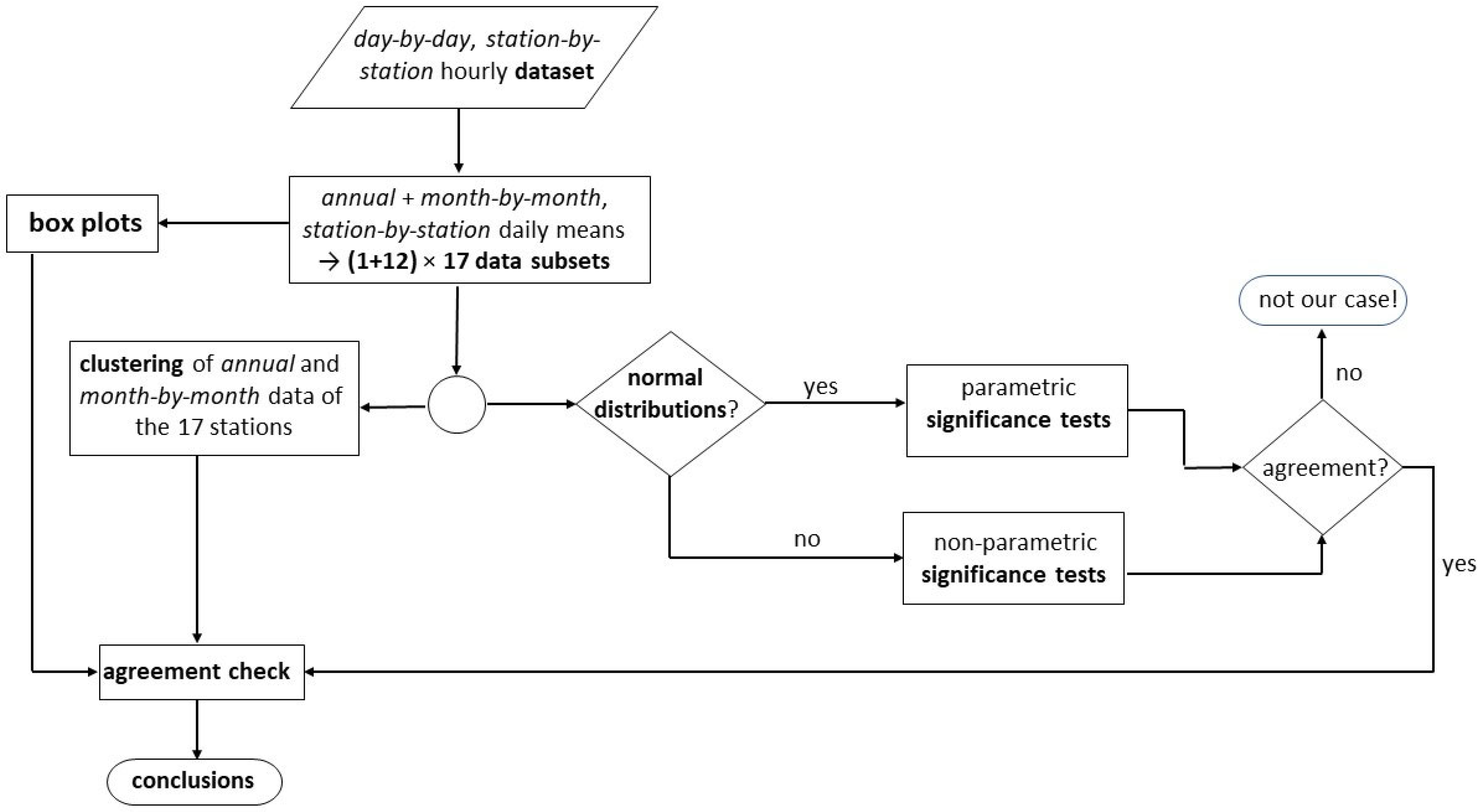
The path of the elaboration of the data devoted to achieving the results reported and discussed in Section 3 is outlined in Figure 2, as complemented by Schemes S1 and S2. In Figure 2, an essential flow-chart is reported that illustrates the different steps of the organisation of the original dataset and its subsequent statistical treatment. More details regarding the individual steps of the whole process are presented in Schemes S1 and S2.

The unsupervised clustering classification technique was adopted to identify groups of datasets exhibiting different degrees of similarity. A hierarchical procedure to join the datasets into groups was adopted, whereby the complete linkage method was applied and the Euclidean distance between two clusters was used as a similarity metric [25,27,28].

Significance tests were performed using parametric and non-parametric methods. Parametric tests require normal distributions for the population from which the samples are supposed to be extracted. Non-parametric tests do not require such an assumption; therefore, they are suitable for treating non-normally distributed data. Kolmogorov–Smirnov tests for assessing the normality of the distribution were performed in advance, in order to ascribe validity to the parametric tests performed. In most cases, the normality of distribution gave a positive answer at a high enough confidence level (α = 0.05), allowing us to faithfully apply, for the successive analysis, ANOVA parametric tests, in addition to non-parametric Kruskal–Wallis tests. Parametric t-tests and non-parametric Mann–Whitney tests were used to perform comparisons of means or medians, respectively, of two different datasets. Parametric ANOVA and ranking-based Kruskal–Wallis non-parametric tests [25,26] were used to compare the mean values or medians, respectively, relative to differently formulated datasets. It should be noted that the ANOVA parametric test is considered a robust method, providing results that are insensitive to moderate deviations from the assumptions of normal distribution and of equal variances of the datasets submitted for analysis. Unless definitely rejected by the relevant tests, we exploited such a virtue, as long as the conclusions were consistent with those of other tests.

As concerns parametric tests, each dataset was preliminarily subjected to the Grubb test in order to check for the presence of outliers; the few values classified as outliers were eliminated.

According to accepted standard procedures, significance tests checking differences between means or medians aim to evaluate the confidence level, in terms of the probability of being wrong, at which the null hypothesis (H₀) may be rejected. Unless otherwise specified, the commonly adopted 5% probability of being wrong in rejecting H₀ constitutes the border value, as accounted for by the p-value given by the MINITAB^® 22.1 software. Consistently, the acceptance or rejection of H₀ will be operatively assumed for p-values above or below the critical α value of 0.05, respectively.

Whenever plausible, the parallel application of non-parametric and parametric tests allowed for safer conclusions to be drawn from the results of the two different types of tests.

It should be noted that suitable improvements to the classical approaches using one-way ANOVA were proposed in recent years, in order to make ‘rigid’ statistical algorithms free from assumptions that render them poorly useful in many practical applications. Here, we make specific references to the methods adopted in the MINITAB^® software package, which are supposed to implement variations to the standard techniques, in order to achieve best effectiveness, through the request of less-strict conditions to the samples of the data. The Welch test [29] was adopted in the ANOVA analysis, which, at variance with the F-test, is effective in minimising false positives when working on samples with unequal variance. Furthermore, in order to identify the samples that do differ from the others, a multiple comparison method is implemented in MINITAB^® Statistical Software as a form of post-ANOVA treatment [30]. It also combines the control for the increased error that occurs when making multiple comparisons [31] with the possible unequal size of the samples [32] into the Games–Howell method, which does not assume equal standard deviations for the samples of data [33]. Adjustments are performed when comparing the differences in each pair of means. In our treatment, ANOVA was integrated with the subsequent post-ANOVA Games–Howell pairwise multiple comparison procedures, which allowed us to group stations and months possessing non-significantly different means. In an analogue way, the Kruskal–Wallis test, when the null hypothesis is rejected, may be followed by the Dunn test [34], which is the non-parametric pairwise multiple comparison procedure for the differences in the medians [35].

Most often, the samples under examination were analysed in parallel using both parametric and non-parametric tests; the agreement between the conclusions of the two kinds of tests was checked. Similarly, despite the fact that the results of techniques belonging to different typologies are involved, we could satisfactorily compare the results gained using the clustering technique with those obtained using the ANOVA technique, as supported by the cited post-ANOVA tests.

As regards the actual meaning of the classification currently adopted by the administrative authorities, ANOVA and Kruskal–Wallis tests were applied to the data obtained from groups of stations of the same typology, i.e., RB, SB, UB, and UT stations belonging to different provinces, in order to check whether they could be considered comparable.

3. Results and Discussion

The choice to analyse data collected during the day, i.e., from 06 a.m. to 12 p.m., rather than from the whole 24 h period, limited only to working days, is supported by statistical significance tests, both parametric and non-parametric in character, i.e., one-tailed t-tests and Mann–Whitney Rank Sum tests, respectively.

3.1. Spatial and Temporal Distributions of NO₂ Concentrations

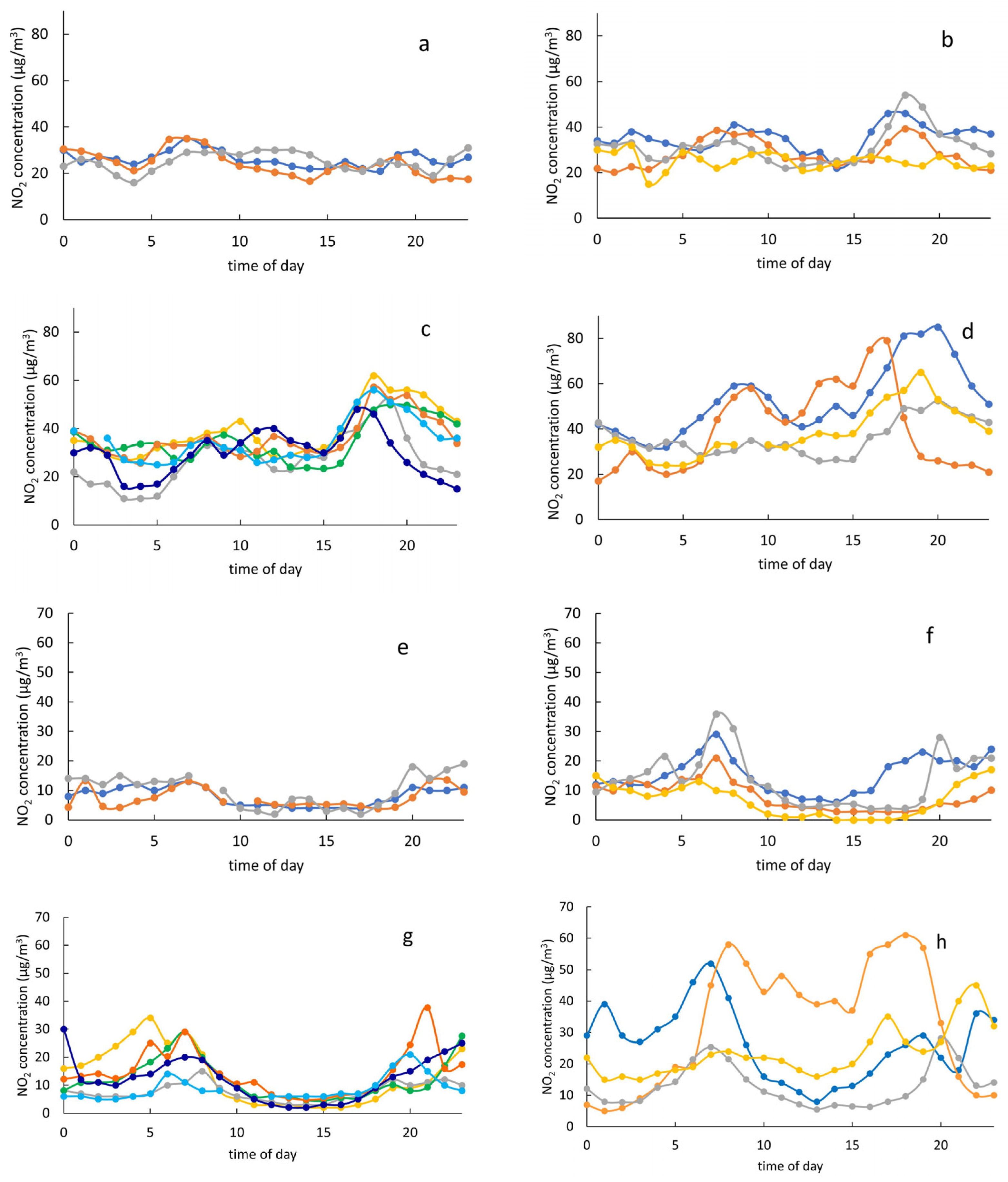
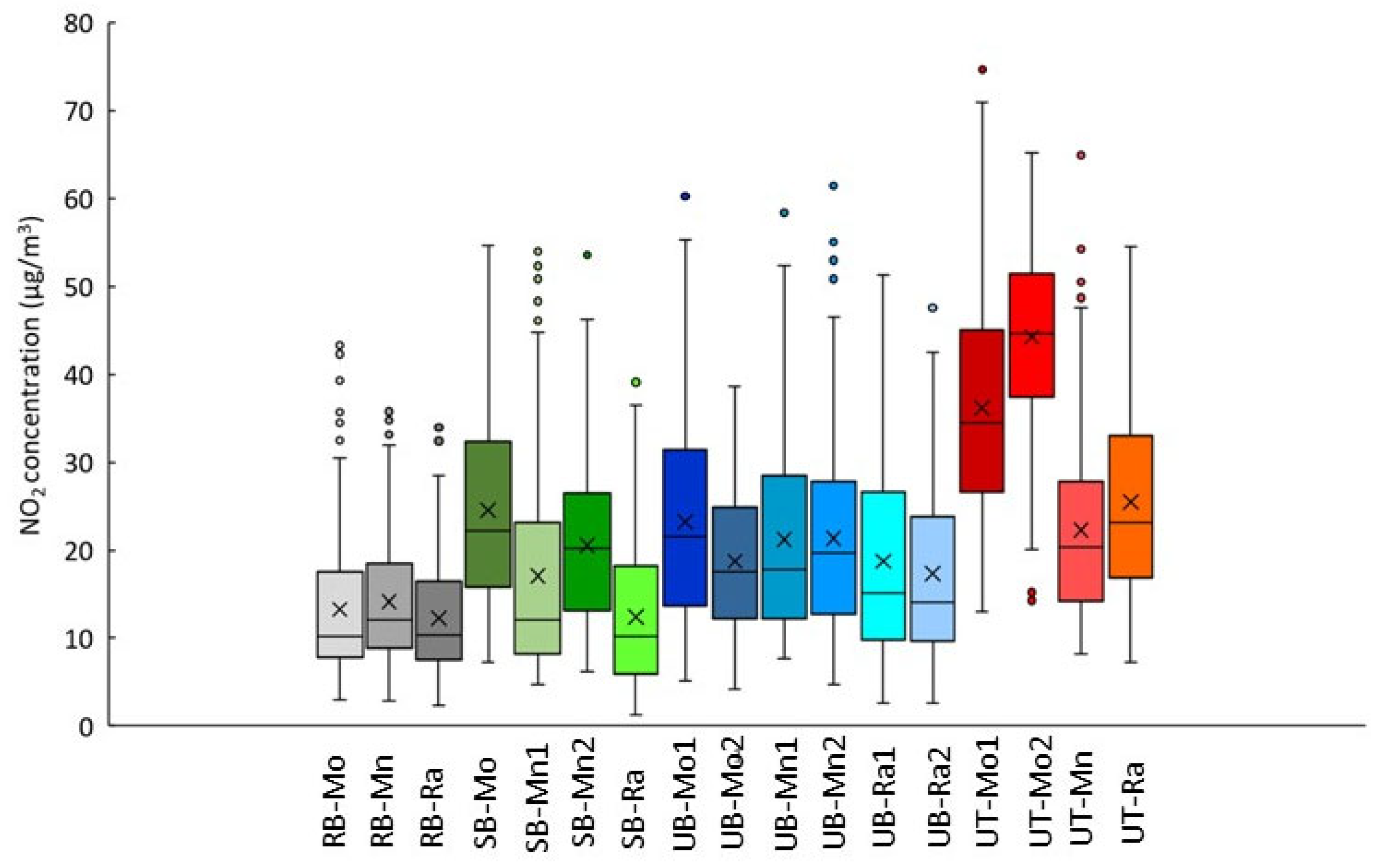
The daily measurements collected in the different stations over two days, taken as being representative of the winter and summer seasons, respectively, are plotted in Figure 3. The box plot relative to the data collected in any stations, day-by-day throughout the whole year, in the range 06 a.m. to 12 p.m., is reported in Figure 4. General indications, which cannot be contradicted even by sound significance tests, are given by the trends exhibited in these plots. Table S1 collects the values of the relevant median, first, and third quartiles, together with the mean, minimum, and maximum values, which are taken from the box plot in Figure 4, with the addition of the estimated standard deviation value. Interesting indications of the extent of the difference in the distributions relative to the annual data for each station are given by the median values, which vary from 10.21 to 44.58 μg/m³, and by the interquartile range values, taken as an indication of the width of the distribution, which vary between 8.92 and 18.42 μg/m³.

At first sight, it seems evident that the results of chemical analyses do not show clear agreement with the criteria adopted for the distinction made in the four cited classifications of the monitoring sites, i.e., RB, SB, UB, and UT. With this in mind, a more detailed analysis for the achievement of significant conclusions is mandatory.

In particular, as relates to the similarity between data from stations of the same typology, on the one hand, quite similar contents of NO₂ in the air are detected in all the RB monitoring stations, while not particularly remarkable differences are presented within the UB stations. On the other hand, the SB stations do not seem to constitute a homogeneous group, with SB-Ra being more similar to RB stations, and being hardly comparable to the SB-Mo station; this emerges as the most polluted station in this category. The most marked differences can be observed within the UT group, where both stations in Modena, i.e., UT-Mo1 and UT-Mo2, appear to be the most polluted by NO₂, compared to all the other stations. On the contrary, UT-Mn presents a surprisingly low value, which is quite similar to UB-Mn1 and UB-Mn2.

The box plots representing the annual data evidence the presence of many outliers. These are often relative to specific months (namely, a high number of outliers is detected in January), which suggests a reasonable dependence of the pollutant concentrations on the season. This seems a key point to consider, in view of proposed actions to contrast air pollution and vehicle traffic and, in general, combustion processes. In the frame of programming possible interventions for mitigation, the meaning of the box plots accounting for the data over the whole year is, in fact, insufficient to provide a complete picture.

Further information may be gained via an analysis of the station-by-station monthly data. For this reason, the whole dataset relative to the NO₂ concentrations measured in the monitoring stations is summarised, month by month; the statistical data are reported in Tables S2–S13. The low dispersion of data found within the category of the three RB stations on the basis of annual evaluations is also observed across the months. Although they also often present the lowest values, in summer months, they show comparable values to some SB stations.

The most heavily polluted sites for every month of the year are confirmed to be the two UT stations in the province of Modena, i.e., UT-Mo1 and UT-Mo2, which are both characterised by particularly high traffic levels (33,000 and 26,000 vehicles/day, respectively, in 2022) [36]. The monthly data of the other UT stations, namely UT-Mn and UT-Ra, in a similar pattern as is observed for their annual behaviour, always indicate lower NO₂ levels, which are often comparable, if not even lower, to those measured in the UB stations and in some SB stations. No evident differences between the UT-Mn station and UB-Mn1, both located in the city of Mantova, are shown over most months of the year.

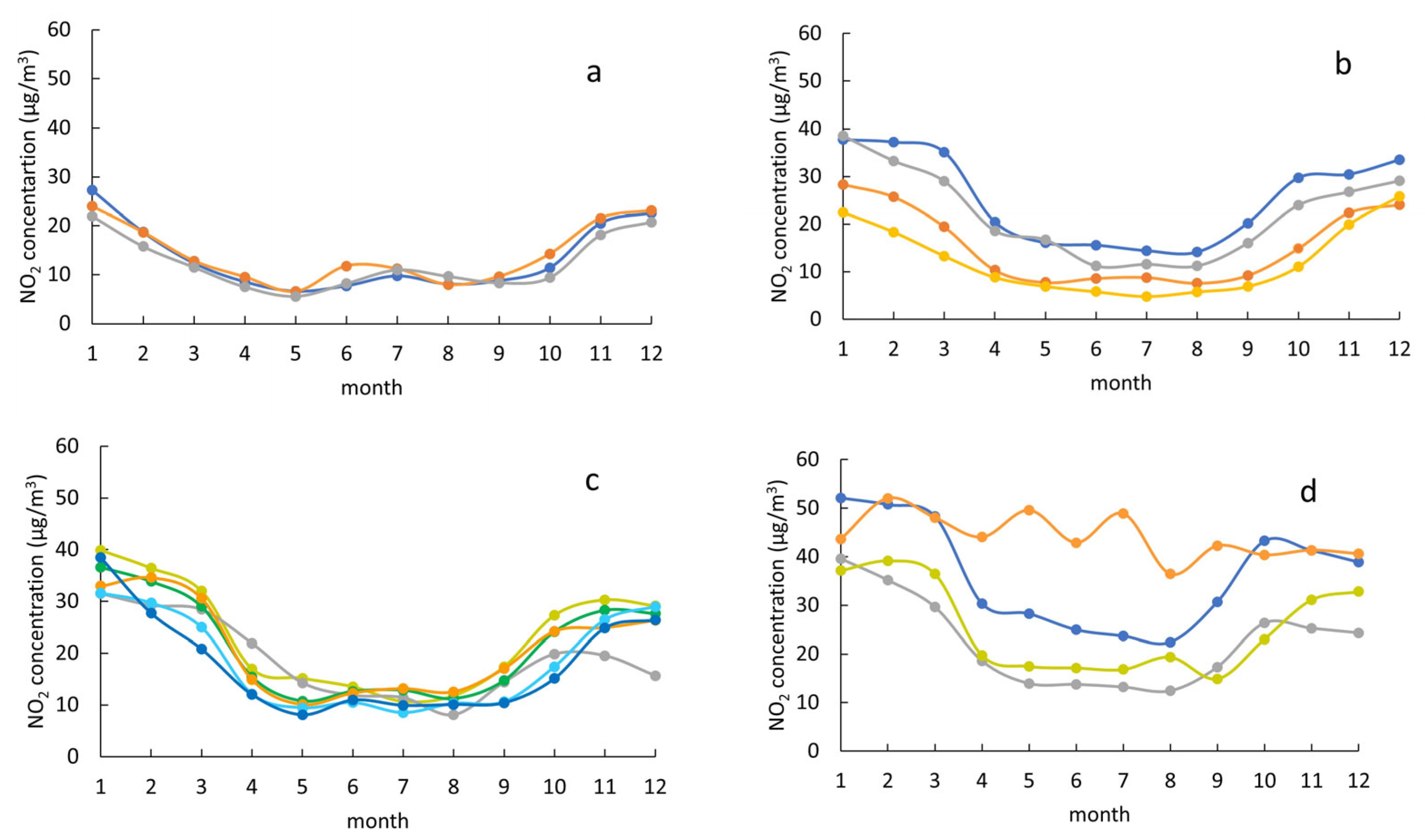
Figure 5 reports the month-by-month trends in the mean daily measurements for the different stations. In general, all stations exhibit similar seasonal trends over the year, i.e., a progressive decrease from January, February, and March to the summer months, and a subsequent increase from September onwards. Then, nearly constant values are observed, before a return to the highest values measured within the year.

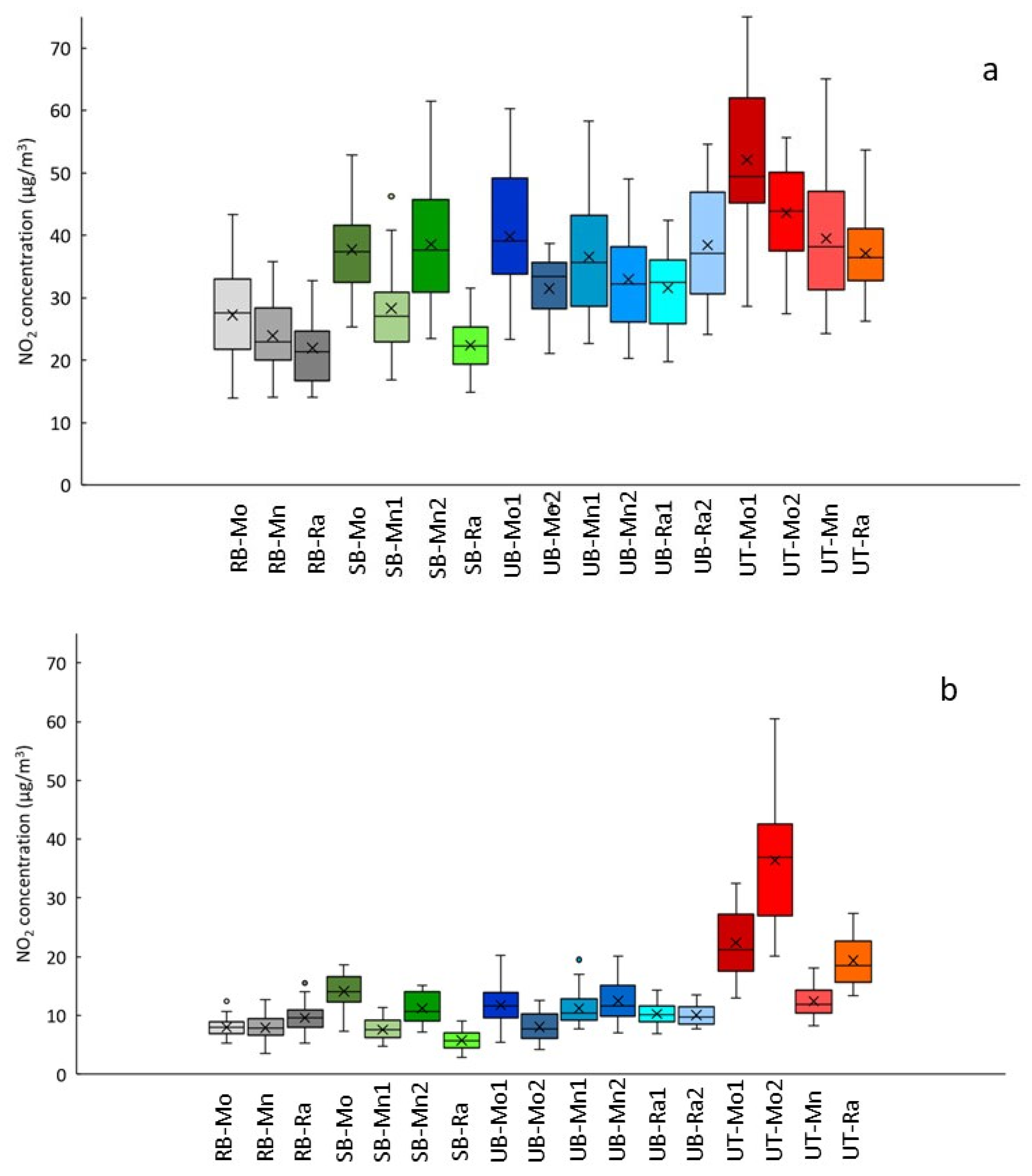
A complete picture of the evolution of the situation over time is given by the box plots of the individual stations that are reported across the months in Figures S1–S4. As examples, the box plots for all stations in January and August are depicted in Figure 6. Similar plots give further support to the conclusion that all the UT stations of the three provinces, with the exception of UT-Mo2, exhibit the highest NO₂ pollution during the winter months.

3.2. Cluster Analysis

After this preliminary exam, based on the box plots and summary statistics, a further step, according to a key goal of the work, was enacted to evaluate the data from a more statistically meaningful viewpoint in order to test the possible agreement of the currently adopted classification of the stations with the results of chemical monitoring. In this way, as first steps, checks were carried out relating to (i) the actual significance of the difference among categories, as ascribed to the monitoring stations within the same province, and to (ii) the absence of meaningful differences among data from sites ascribed to the same category, in the three provinces. The importance of such an exam, even in a more general frame with respect to the specific case under study, is evident when considering the added value of a reliable comparison between monitoring data that are relative to the different provinces. Ultimately, in view of the transferability of the results of the monitoring procedure as a whole, this comparison should be made considering the preliminary experimental design, the measurement process, and the final data analysis.

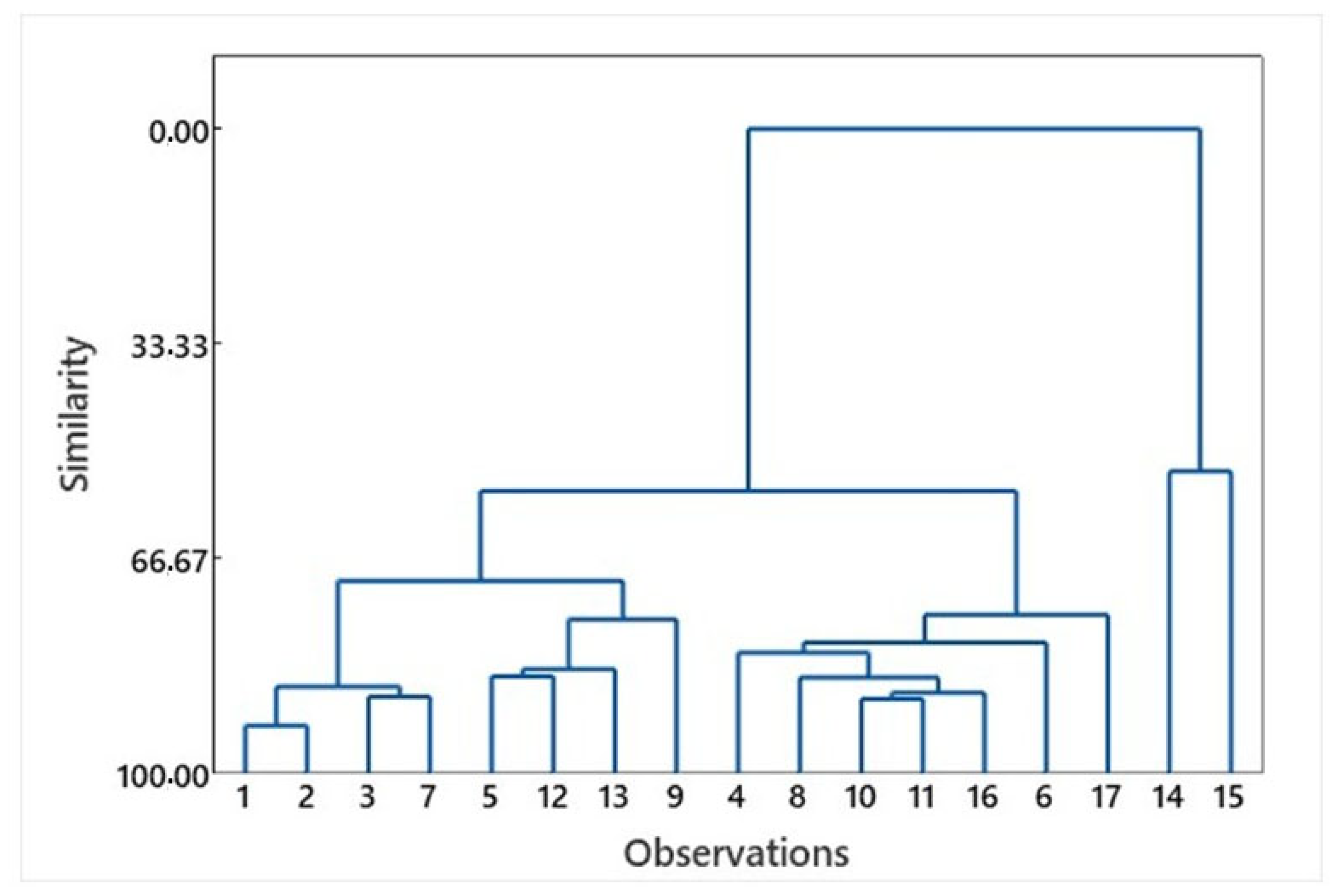
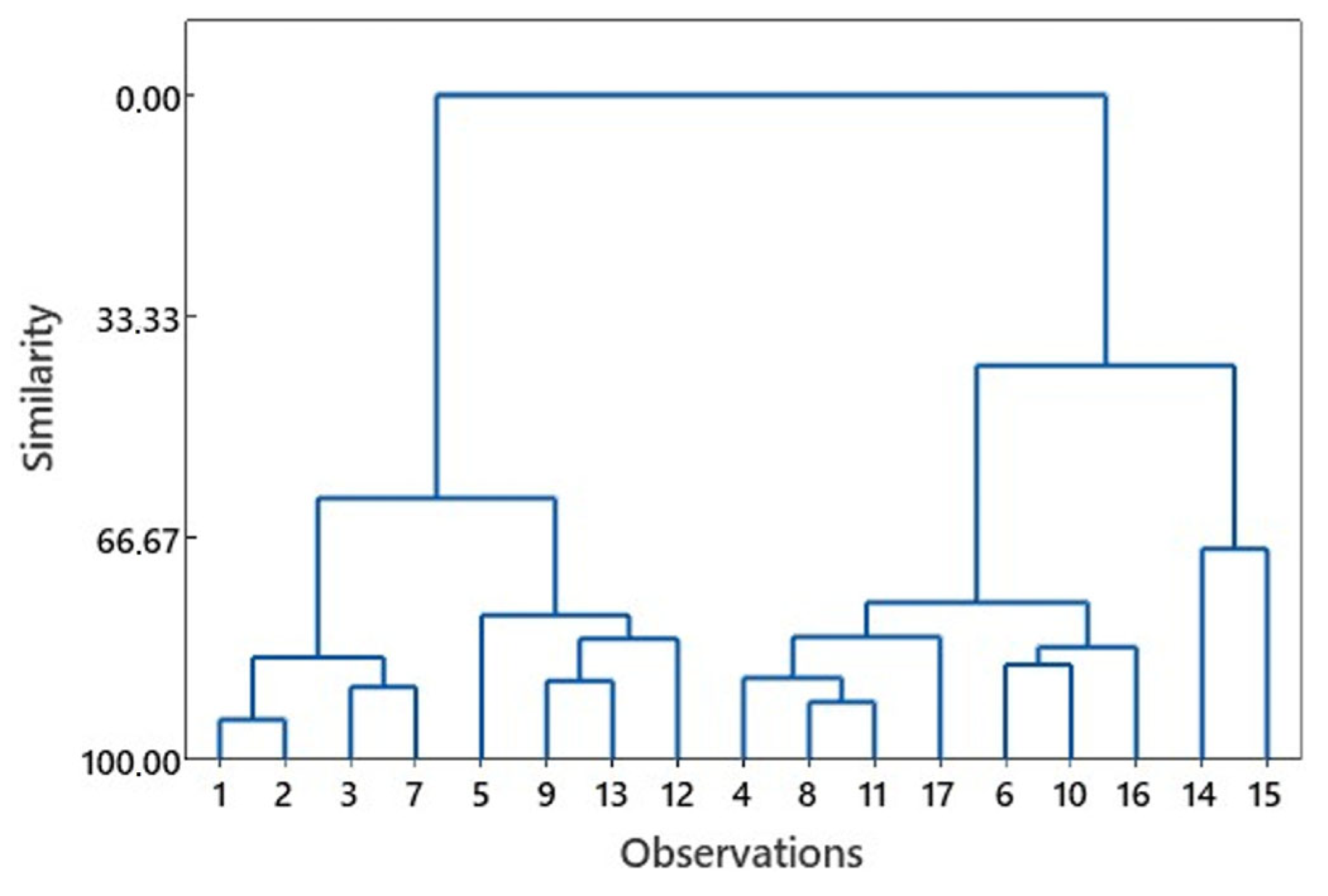
For this purpose, in order to find possible similarities among the data from stations that are classified differently and are located in different provinces, i.e., among the whole of the 17 stations, unsupervised cluster analyses were performed on the yearly and monthly data of the 17 stations. The dendrogram relative to the annual data is reported in Figure 7.

A rigorous exploration of the dendrogram in Figure 7, in terms of the levels of similarity at which subsequent clustering steps occur, leads to the data that are presented in

Table 2. Clusters formed in successive amalgamation steps, according to the dendrogram in Figure 7. The order accounts for progressive decrease in similarity levels, i.e., from the individual objects to clusters grouping a higher and higher number of objects. The decreasing values of the similarity levels are also reported, at which the progressive grouping of the subgroups of the specified composition occur.

Step	Number of Clusters	Similarity Level (%)	Clusters Joined		New Cluster	Number of Obs. in New Cluster
1	16	92.5	1	2	1	2
2	15	88.5	10	11	10	2
3	14	88.1	3	7	3	2
4	13	87.5	10	16	10	3
5	12	86.5	1	3	1	4
6	11	85.1	8	10	8	4
7	10	85.0	5	12	5	2
8	9	83.8	5	13	5	3
9	8	81.2	4	8	4	5
10	7	79.7	4	6	4	6
11	6	76.1	5	9	5	4
12	5	75.4	4	17	4	7
13	4	70.1	1	5	1	8
14	3	56.2	1	4	1	15
15	2	53.1	14	15	14	2
16	1	0.0	1	14	1	17

.

In order to present a more accessible picture of the more-or-less effective grouping of the 17 monitoring stations depicted in the dendrogram,

Table 3. Clusters derived from the dendrogram reported in Figure 7.

Number of Clusters	Composition of the Clusters	Similarity Level (%)
1	1 2 3 4 5 6 7 8 9 10 11 12 13 14 15 16 17	0
2	1 2 3 4 5 6 7 8 9 10 11 12 13 16 17–14 15	0–53.1
3	1 2 3 4 5 6 7 8 9 10 11 12 13 16 17–14-15	53.1–56.2
4	1 2 3 5 7 9 12 13–4 6 8 10 11 16 17–14-15	56.2–70.1
5	1 2 3 7–5 9 12 13–4 6 8 10 11 16 17-14-15	70.1–75.4
7	1 2 3 7–5 12 13–9–4 6 8 10 11 16–17–14-15	75.4–79.7

reports the clusters that are evident within a narrow enough range of similarity levels, rather than at exact similarity values. Note that in Table 3,

Table 4. Clusters derived from the dendrogram reported in Figure 8.

Number of Clusters	Composition of the Clusters	Similarity Level (%)
1	1 2 3 4 5 6 7 8 9 10 11 12 13 14 15 16 17	0
2	1 2 3 5 7 9 12 13–4 6 8 10 11 14 15 16 17	0–40.698
3	1 2 3 5 7 9 12 13–4 6 8 10 11 16 17–14 15	40.68–60.66
4	1 2 3 7–5 9 12 13–4 6 8 10 11 16 17–14 15	60.66–68.32
7	1 2 3 7–5 9 12 13–4 6 8 10 11 16 17–14–15	68.32–76.42

and

Table 5. Clusters derived from the dendrogram reported in Figure 9.

Number of Clusters	Composition of the Clusters	Similarity Level (%)
1	1 2 3 4 5 6 7 8 9 10 11 12 13 14 15 16 17	0
2	1 2 3 4 5 6 7 8 9 10 11 12 13 14 16 17–15	0–53.24
3	1 2 3 4 5 6 7 8 9 10 11 12 13 16 17–14-15	53.24–72.22
4	1 3 5 7 12–2 4 6 8 9 10 11 13 16 17-14-15	72.22–84.40
5	1 3 5 7 12–2 6 8 9 10 11 13 16–4 17-14-15	84.40–88.52

, the increase in the number of clusters identified implies increasing values of the similarity levels. The order along which the dendrogram is read is the opposite of that in Table 2.

Cluster analysis has been used by several authors to analyse and optimise air monitoring networks [37,38,39]. As regards the dendrogram relative to the whole year (Figure 7), which is analysed in Table 3, at around a similarity level of 70–75%, three clusters are identified, corresponding to increasing levels of NO₂ concentrations. The first cluster includes all RB stations and one SB station; the second cluster includes a few UB stations and one SB station; the third cluster includes the other UB stations, one SB station, and two UT stations, namely UT-Mn and UT-Ra. As regards the other UT stations, UT-Mo1 and UT-Mo2 are linked and form a separate cluster at a lower level of similarity (53%). We can observe that the same category of stations is not always included in the same clusters, apart from the case of the RB stations.

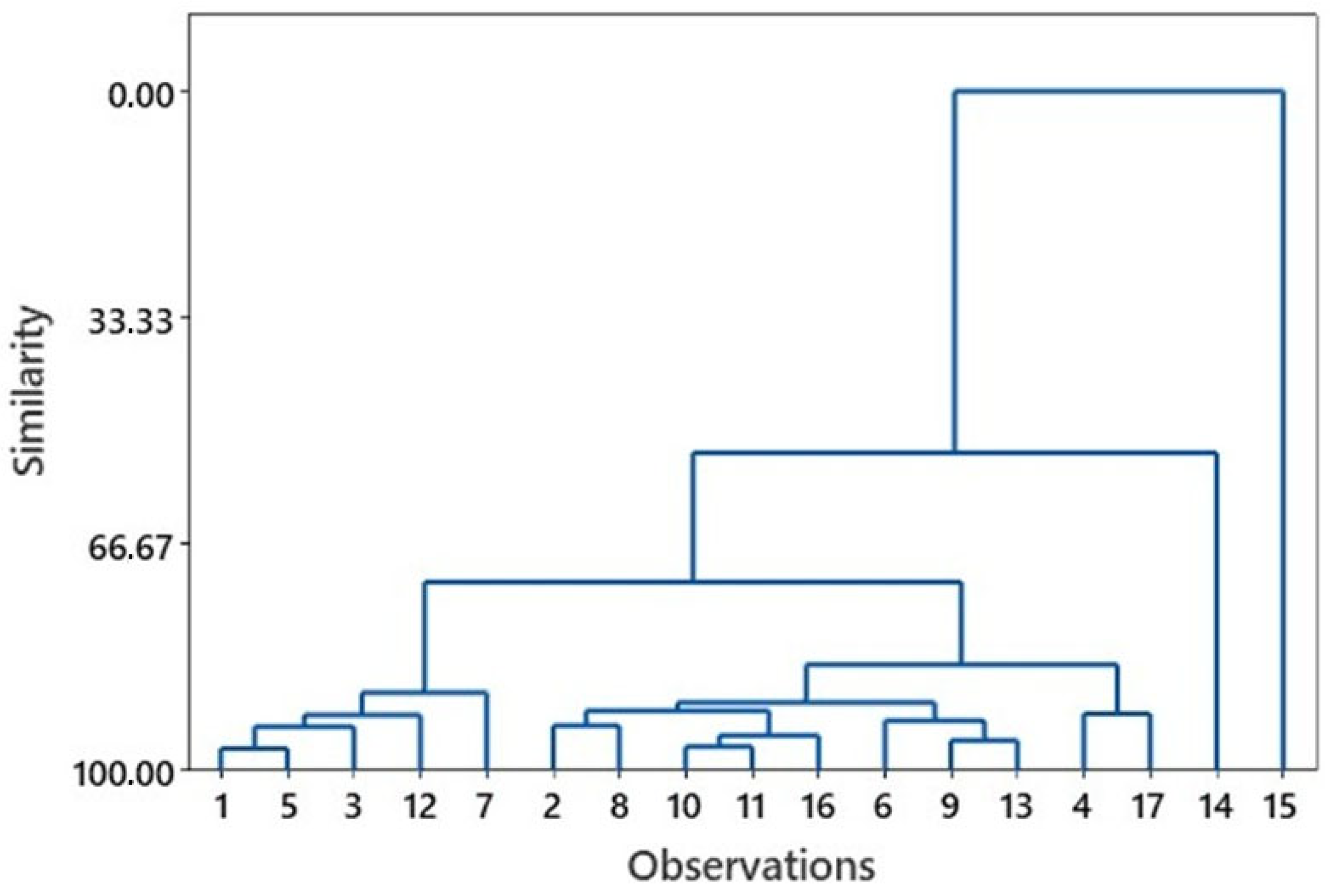
Similar cluster analyses were performed on the data from single months. As examples, the dendrograms relative to February and June are presented in Figure 8 and Figure 9 and the deduced compositions of the clusters are depicted in Table 4 and Table 5. The dendrograms and the consequent clusters relative to the other single months are reported in Figures S5–S14 and Tables S14–S23, respectively.

On the basis of comparable similarity ranges, which are suitable for identifying different clusters in the dendrograms of the different months, groupings of the different stations may be discussed. The clustering of the monthly datasets, with the exception of July and October, amalgamates all the RB stations in the same group at a similarity level higher than 75%. The SB stations confirm their heterogeneity. On the one hand, the less-polluted stations, i.e., SB-Mn1 and SB-Ra, are most often clustered together with the RB stations; on the other hand, SB-Mo and SB-Mn2 are included in a different group. In a similar way, the six UB stations are always distributed in different clusters, although they are never amalgamated with the RB stations and the two most-polluted UT stations. As regards the UT stations, two of them, i.e., UT-Mo1 and UT-Mo2, are always separated from the other UT ones. In particular, from May to August, the UT-Mo2 station is not clustered with any other station. This fact can be accounted for by the high levels of NO₂ concentrations that are detected by this station throughout all the months of the year. A peculiar behaviour is shown by the UT-Mn station, which is always included in the same cluster as UB-Mn1, which is the urban background station located in the same city.

The analysis of the dendrograms relative to the cold months, namely January, February, March, November, and December, is very similar to that of the annual dendrogram shown in Figure 7 and analysed in Table 3. As an example, at 70–72% similarity levels, three or four clusters are identified in February (Figure 8 and Table 4).

From April to October, the identification of at least three clusters occurs at higher levels of similarity compared to those found in the other months of the year. As an example, the dendrogram relative to June and the clusters derived from it, as reported in Figure 9 and Table 5, respectively, indicate that the groups formed are all highly heterogeneous as to the categories currently adopted.

It should be noted that the results from the unsupervised pattern recognition clustering technique are in good agreement with what was deduced and critically discussed with respect to the box plot representations.

3.3. Significance Tests: Comparison of NO₂ Concentrations in Different Stations

The preliminary exam carried out thus far can be further validated using suitable statistical tests, which aim to achieve conclusions with sound statistical significance. First of all, the normality of the data distribution was checked using the Kolmogorov–Smirnov method in order to choose the appropriate tests. The results (Table S24) demonstrate that almost all monthly data relative to each station are normally distributed at a 0.05 significance level. Although most annual data do not fit a normal distribution at such a significance level thanks to the cited property of ANOVA in terms of its insensitiveness or moderate deviations from the assumption of a normal distribution of the data, we chose to use both parametric and non-parametric tests. One-way ANOVA, Kruskal–Wallis, post-ANOVA, and Dunn tests were employed.

As a first step, in view of the seasonal peculiarities, the annual and the monthly datasets of all the seventeen stations were analysed; as expected, the one-way ANOVA and Kruskal–Wallis tests rejected the null hypothesis that affirms that the mean or the median values, respectively, are equal to one another. The multiple comparison procedure based on the Games–Howell post-ANOVA method was applied to obtain further information about which stations can be grouped as being non-significantly different from each other at the 0.05 significance level. As examples, the results relative to the February and June datasets are reported in

Table 6. Post-ANOVA grouping of the stations under examination, as indicated using the Games–Howell method, at the 0.05 significance level. The monthly N data used are the daily mean NO₂ concentrations in February 2022. Means of NO₂ concentrations that do not share a letter are significantly different.

Station	ID	N	Mean (μg/m3)	Grouping
UT-Mo2	15	24	52.04	A
UT-Mo1	14	24	50.76	A
UT-Ra	17	24	39.13		B
SB-Mo	4	24	37.21		B	C
UB-Mo1	8	24	36.42		B	C
UB-Mn2	11	24	34.59		B	C	D
UB-Mn1	10	24	33.84		B	C	D	E
UT-Mn	16	23	33.82		B	C	D	E
SB-Mn2	6	24	33.27		B	C	D	E
UB-Ra1	12	24	29.67			C	D	E
UB-Mo2	9	24	29.25			C	D	E
UB-Ra2	13	24	27.71				D	E
SB-Mn1	5	24	25.70					E	F
RB-Mo	1	24	18.70						F	G
RB-Mn	2	24	18.67						F	G
SB-Ra	7	24	18.33						F	G
RB-Ra	3	24	15.76							G

and

Table 7. Post-ANOVA grouping of the stations under examination, as indicated using the Games–Howell method, at the 0.05 significance level. The monthly N data used are the daily mean NO₂ concentrations in June 2022. Means of NO₂ concentrations that do not share a letter are significantly different.

Station	ID	N	Mean (μg/m3)	Grouping
UT-Mo2	15	25	42.88	A
UT-Mo1	14	25	24.93		B
UT-Ra	17	24	17.13			C
SB-Mo	4	25	15.57			C
UT-Mn	16	25	13.73			C	D
UB-Mo1	8	25	13.51			C	D	E
UB-Mn1	10	25	12.60				D	E
UB-Mn2	11	25	12.29				D	E
UB-Mo2	9	25	11.84				D	E
RB-Mn	2	25	11.76				D	E
SB-Mn2	6	25	11.20				D	E	F
UB-Ra2	13	25	10.94				D	E	F
UB-Ra1	12	24	9.86					E	F	G
SB-Mn1	5	25	8.60						F	G
RB-Ra	3	25	8.15						F	G
RB-Mo	1	24	7.41							G	H
SB-Ra	7	24	5.47								H

; the results relative to the other monthly data are reported in Tables S25–S34.

In general, the groups of stations, which are formed through the application of the Games–Howell pairwise comparison method, are consistent with the results of the clustering process. The results reported in Table 6 and Table 7, as representative examples, indicate that the mean data of the stations that are not significantly different according to the Games–Howell post-ANOVA method are the same as those that are included in the groups identified using the clustering technique (Table 4 and Table 5). In particular, in February, the first cluster coincides with group G in the Games–Howell grouping, the second cluster coincides with group E, the third cluster coincides with group B, and the fourth cluster coincides with group A. In June, an analogous correspondence can be observed; the separation of the UT-Mo1 and UT-Mo2 stations is evidenced from both the results of clustering and from the Games–Howell grouping.

As concerns the annual data, considering the non-normal distribution of most datasets, in addition to the Games–Howell test (

Table 8. Post-ANOVA grouping of the stations under examination, as indicated using the Games–Howell method, at the 0.05 significance level. The annual N data used are the daily mean NO₂ concentrations in 2022.

Station	ID	N	Mean (μg/m3)	Grouping
UT-Mo2	15	296	44.24	A
UT-Mo1	14	304	36.13		B
UT-Ra	17	296	25.45			C
SB-Mo	4	302	24.56			C	D
UB-Mo1	8	304	23.23			C	D	E
UT-Mn	16	303	22.15				D	E
UB-Mn2	11	303	21.24					E	F
UB-Mn1	10	304	21.22					E	F
SB-Mn2	6	299	20.57					E	F
UB-Ra1	12	304	18.75						F	G
UB-Mo2	9	301	18.74						F	G
UB-Ra2	13	302	17.30							G
SB-Mn1	5	304	17.10							G
RB-Mn	2	304	14.15								H
RB-Mo	1	299	13.20								H	I
SB-Ra	7	299	12.41								H	I
RB-Ra	3	300	12.23									I

), pairwise multiple comparisons were performed using the Dunn test (

Table 9. Grouping of stations using the Dunn method at the 0.05 significance level. The N data used are the daily mean NO₂ concentrations in 2022.

Station	ID	N	Mean (μg/m3)	Grouping
UT-Mo2	15	296	44.24	A
UT-Mo1	14	304	36.13		B
UT-Ra	17	296	25.45			C
SB-Mo	4	302	24.56			C	D
UB-Mo1	8	304	23.23				D	E
UT-Mn	16	303	22.15					E
UB-Mn2	11	303	21.24					E
UB-Mn1	10	304	21.22					E
SB-Mn2	6	299	20.57					E
UB-Ra1	12	304	18.75						F
UB-Mo2	9	301	18.74							G
UB-Ra2	13	302	17.30						F	G	H
SB-Mn1	5	304	17.10								H
RB-Mn	2	304	14.15									I
RB-Mo	1	299	13.20									I	J
SB-Ra	7	299	12.41										J
RB-Ra	3	300	12.23										I

). However, the results obtained using the Dunn test are less consistent, compared to results of the Games–Howell test, with the clustering procedure. This may be not surprising in view of the lower sensitivity and recognition capability of the non-parametric techniques, which work on ranks rather than on precise values.

As a second step, both ANOVA and Kruskal–Wallis tests were performed on stations belonging to the same category, i.e., four UT sites; six UB sites; four SB sites; and three RB sites. Statistical analyses were performed on the monthly data in addition to the annual data. The results are summarised in

Table 10. Comparison of daily NO₂ mean concentrations in RB, SB, UB, and UT stations in the provinces of Modena, Mantova, and Ravenna: p-values from one-way ANOVA based on the Welch test and the Kruskal–Wallis test are reported. p-values that do not allow for the rejection of H₀, at a significance level of 0.05, are in bold.

	p-Value from Welch Test				p-Value from Kruskal–Wallis Test
Period	RB Stations	SB Stations	UB Stations	UT Stations	RB Stations	SB Stations	UB Stations	UT Stations
Annual	0.002	0.000	0.000	0.000	0.000	0.000	0.000	0.000
January	0.051	0.000	0.001	0.000	0.057	0.000	0.004	0.000
February	0.136	0.000	0.001	0.000	0.121	0.000	0.001	0.000
March	0.429	0.000	0.000	0.000	0.554	0.000	0.000	0.000
April	0.028	0.000	0.000	0.000	0.050	0.000	0.000	0.000
May	0.055	0.000	0.000	0.000	0.112	0.000	0.000	0.000
June	0.000	0.000	0.005	0.000	0.000	0.000	0.003	0.000
July	0.038	0.000	0.000	0.000	0.165	0.000	0.000	0.000
August	0.014	0.000	0.000	0.000	0.014	0.000	0.000	0.000
September	0.052	0.000	0.000	0.000	0.098	0.000	0.000	0.000
October	0.000	0.000	0.000	0.000	0.000	0.000	0.000	0.000
November	0.108	0.000	0.000	0.000	0.078	0.000	0.000	0.000
December	0.277	0.000	0.000	0.000	0.214	0.000	0.000	0.000

. Except for the RB stations, which, in most months, do not show significant differences from one another, all other categories of stations, i.e., SB, UB, and UT, do not constitute three well-defined homogeneous groups that are different from each other. This confirms that the classification currently adopted, as well as the relevant denomination of the stations, does not always account for different objective situations with respect to NO₂ air pollution, as is indisputably assessed in the chemical analyses. One-way ANOVA based on the Welch test and the Kruskal–Wallis test lead to comparable results for the two statistical approaches, for any groups of stations and any months, with the only exception being shown in Table 10.

The pairwise multiple comparison post-ANOVA procedure using the Games–Howell method at a 95% confidence level was applied to data relating to SB, UB, and UT stations, for which the one-way ANOVA procedure always rejects the null hypothesis; the results are reported in Table S35. These results confirm the previous observations based on box plots and cluster analysis, whereby each category of stations constitutes a heterogeneous group. In particular, the SB and UT stations are divided, with a few exceptions, into three or four groups, which are characterised by non-significantly different NO₂ mean concentrations.

Similar significance tests were performed considering, province by province, (i) six MO; (ii) six MN; and (iii) five RA stations. The possible identification of a progressive increase in NO₂ pollution from RB to UT stations is not evidenced in the results obtained using the Games–Howell grouping reported in Table S36. In the province of Modena, the pairwise multiple comparisons indicate that the stations that are not significantly different can be gathered into different groups (from three to five); however, there are no cases whereby these stations belong to the same category. In the province of Mantova, a low number of groups are identified (two or three); therefore, in general, UT-Mn, UB-Mn1, and UB-Mn2 do not show significant differences for most months of the year, suggesting that poor differences characterise the various stations. On the other hand, in the province of Ravenna, in most months, the UB stations form a different group with respect to the UT station; the SB station is not significantly different from the RB one but, in most cases, is separated from the UT and UB stations.

In a few seemingly anomalous cases, t-tests and Mann–Whitney tests were used to draw conclusions about the differences between data from stations belonging to different categories. In particular, data relative to the main cities of the provinces have attracted our attention; the results of a few significant comparisons are reported in

Table 11. Comparison between UT and UB stations located in the same city (Modena, Mantova, and Ravenna) based on t-tests and Mann–Whitney tests. p-values that do not allow for the rejection of H₀, at a significance level of 0.05, are in bold.

	t-Test			Mann–Whitney Test
Period	UT-Mo1/ UB-Mo1 p-Value	UT-Mn/ UB-Mn1 p-Value	UT-Ra/ UB-Ra1 p-Value	UT-Mo1/ UB-Mo1 p-Value	UT-Mn/ UB-Mn1 p-Value	UT-Ra/ UB-Ra1 p-Value
Annual	0.000	0.273	0.000	0.000	0.109	0.000
January	0.000	0.305	0.054	0.002	0.327	0.047
February	0.000	0.993	0.000	0.000	0.774	0.000
March	0.000	0.829	0.000	0.000	0.836	0.000
April	0.000	0.000	0.000	0.000	0.000	0.000
May	0.000	0.000	0.000	0.000	0.000	0.000
June	0.000	0.128	0.000	0.000	0.140	0.000
July	0.000	0.657	0.000	0.000	0.546	0.000
August	0.000	0.135	0.000	0.000	0.074	0.000
September	0.000	0.021	0.000	0.000	0.017	0.000
October	0.000	0.066	0.000	0.000	0.052	0.000
November	0.000	0.064	0.022	0.000	0.107	0.009
December	0.000	0.009	0.018	0.000	0.015	0.019

. We can observe that, differently from Modena and Ravenna, the data relative to the UT station in Mantova are not significantly different from the data detected in the UB station, as regards the annual dataset and the majority of the monthly datasets. This result suggests that, in Mantova, the location of the UT station may not be a good choice as concerns the representativeness of the pressure of traffic-related pollution.

Following on from the above discussion, the adopted criteria and denominations for the identification of the sites that are suitable for accounting for the different situations encountered in the examined area do not always give a representation of different anthropic pressures. We can observe that only the RB monitoring sites are, in general, different from the sites belonging to different categories; the distinction made between UT, UB, and SB stations does not always correspond to significant differences in NO₂ concentrations. These conclusions are in agreement with those reported in studies concerning the homogeneity of pollutant concentrations in stations belonging to the same category in the Veneto region [40].

A classification of the air quality monitoring stations based on common criteria is of fundamental importance for a shared interpretation of the data, an assessment of the trend in pollutant concentrations, and an estimate of population exposure to specific pollutants [23]. The spatial representativeness of the stations constituting a network is a widely debated problem and its evaluation is directly connected to the classification process. The current monitoring network examined in this study presents clear limits with respect to this, mainly as regards pollutants characterised by high spatial variability, such as NO₂. Indeed, in urban contexts, traffic emissions cause strong gradients of NO₂ concentrations [23]. In particular, the variability in pollution concentration in stations belonging to the same category, even within the same province, can be explained by the substantially subjective criteria adopted to choose the location of the different stations. From this standpoint, the rural stations operating in areas that are relatively far from anthropogenic pollutants are representative of larger areas than the urban ones [38], where punctual emission sources are present; individual traffic stations seem to be very peculiar and poorly representative of the category as a whole.

As a final consideration, all the approaches relating to the results of the analyses of the data relative to air pollution from NO₂ throughout 2022 identify the highest NO₂ concentrations in the colder months, which coincides with the heavy use of vehicles, the activation of heating systems, and, often, with the more intense activity of factories devoted to the production of most kinds of goods. In particular, the increase in traffic volume, compared to the summer period, is a result of several factors, among which we can include the opening of schools and the different meteorological conditions that, currently, still seem to induce preferences of private transport compared to public. The peculiarity of the data of air pollution in the winter season is particularly evident for UT stations and agrees with what is clearly visible by anyone who lives in the Po Valley. Indeed, private vehicle traffic is known to play a significant role in urban mobility; this is a habit that is becoming more and more widely diffused in our societies.

Interestingly, although not surprisingly, a peculiar case consists of the data of a station in the province of Modena, namely UT-Mo2, which is located in the biggest ceramic district in Italy. It does not show clear dependence on the season; the relative distribution data highlight that even during the summer period, the NO₂ concentration levels monitored by this station remain quite high. The only evident decrease occurs specifically in August, constituting the only case in which the median of the concentrations drops below 40 μg/m³. This can be traced back to the strong reduction in industrial activity during this particular month, as well as to the heavy character of the transport that characterises the proximity of this station, which is strongly connected to the activity in the particularly highly energy-intensive factories present in this industrial district. A comparison of the data collected by day and at night (the industrial activity lasts over the whole 24 h period), together with a drop in the NO₂ content at night and on holidays, allows us to roughly identify the contribution of heavy traffic to NO₂ pollution.

A final punctual consideration should be devoted to the outstanding critical situation in the city of Modena, whereby any approaches to data analysis dealing with the UT-Mo1 station evidence a dramatic level of NO₂ pollution.

4. Conclusions

Based on datasets of hourly measurements of the NO₂ concentrations in air during 2022, performed by different monitoring stations in three provinces of northern Italy, this study consisted of analysing the data over the whole year and month-by-month, also possibly evidencing seasonal effects. The data analysis was carried out in a step-by-step manner, applying progressively more powerful and demanding statistical techniques. As a punctual, meaningful observation in this respect, the results obtained from clustering pattern recognition, those from parametric, and those from non-parametric significance tests, are in excellent agreement with one another, pointing to similar conclusions.

The results gained for differently classified monitoring stations often disagree with the distinctions operated by the classification method adopted. It follows that even the transfer of the classification from one province to another presents inconsistencies. The work in this study aims to evidence a few flaws in the location of the monitoring stations, mainly related to the lack of harmonised criteria. In particular, the current monitoring network is far from being exhaustively representative of a complex environmental system such as an urban centre. In fact, one or two stations, as in the cases considered in this work, cannot be in charge of representing the pollution degree of a city with an area of several square kilometres, containing a lot of different local situations. In this respect, it should be emphasised that the adoption of common methodologies, at the European level, for the evaluation of the spatial representativeness and for the consequent choice of the monitoring station siting, appears to be urgent. Independently of the goal of the monitoring action, it is evident that an effective mapping of the NO₂ pollution requires a monitoring network that is dense enough, both in terms of the locations of the stations and the sampling time frequency. The dependence on time, i.e., on the season of the year or even on the time of the day, is of equal importance to the space frequency. The time frequency variable may be important to account for the specificity of a day within a month or of a month within a year, which is the only way not to discard the effect of the season; this may also be crucial in order to consider the effect of the rush hour within a day-long time interval. The consideration of the variations in both variables is mandatory in order to ensure an adequate spatial and temporal representativeness. Interpolation algorithms could allow us to draw a multi-dimensional plot accounting for each variable affecting the data [41]. It is evident that the spatial and temporal resolution degree affects the precision of the multidimensional plot and the consequent accurate estimation of the pollution level at points that are different from those directly involved in the measurements. Of course, the model can be complemented by considering additional variables, such as meteorological parameters and the diffusion and eventual reactivity of the specific pollutant. In this case, more sophisticated models and software are required and different approaches are proposed in the literature in relation to this. In any case, it seems evident that preliminary high spatial and temporal resolution sampling in different potential sites, possibly utilising mobile monitoring stations, constitutes a fundamental step for achieving the most effective location of fixed stations.

In conclusion, the effectiveness of the monitoring step towards environmental sustainability is based on chemical data obtained from a representative monitoring network. This is also obtained via the elaboration of the collected measurements, which are suitable for describing the evolving situations. Proper mitigation strategies for air pollution are based not only on proper mapping but also on the proper treatment of the resulting data. In view of these requirements, the aim of the present contribution has been to outline a path of data treatment that is suitable for furnishing a possible basis and achieving sharable criteria to effectively compare local situations, possibly beyond those specifically considered in the present contribution.