Abstract
Solar irradiance is one of the main factors affecting photovoltaic power generation. The shielding effect of clouds on solar radiation is affected by both type and cover. Therefore, this paper proposes the use of textural features to represent the shielding effect of clouds on solar radiation, and a novel textural convolution kernel of a convolutional neural network, based on grey-level co-occurrence matrix, is presented to extract the textural features of clouds. An integrated ultra-short-term solar irradiance prediction framework is then proposed based on feature extraction network, a clear sky model, and LSTM. The textural features are extracted from satellite cloud images, and the theoretical irradiance under clear sky conditions is calculated based on an improved ASHRAE model. The LSTM is trained with the textural features of clouds, theoretical irradiance, and NWP information. A case study using data from Wuwei PV station in northwest China indicate that the features extracted from the proposed textural convolution kernel are better than common convolution kernels in reflecting the shielding effect of clouds on solar irradiance, and integrating textural features of cloud with theoretical irradiance can lead to better performance in solar irradiance prediction. Thus, this study will help to forecast the output power of PV stations.
1. Introduction
With the increasing proportion of installed photovoltaic (PV) power generation, PV power generation has begun to show a mode of “large-scale decentralised development, low-voltage access, and local consumption” [1]. Compared with centralised PVs, distributed PVs can be installed on buildings and other carriers, which have higher flexibility and can significantly improve the utilisation rate of PV devices [2]. But distributed PV installation sites are scattered with a small installed capacity, which has a greater impact on the stability of the power system [3,4]. Therefore, the accurate power prediction of distributed PVs is of great significance to ensure the reliability of the power system and formulate a power market strategy [5,6]. Although distributed PVs have been developed for a period of time, the historical statistical data are not standardised [7]. Moreover, distributed PVs generally do not measure real-time power but only upload the total power generation data to the power grid [8]. Therefore, it is difficult to establish a power prediction model of distributed PV. The principle of PV power generation involves using electronic components to convert solar radiation energy into electrical energy, and the power can be calculated by the solar irradiance according to the empirical formula. Therefore, the accurate prediction of solar irradiance is the basis for the power prediction of distributed PV power generation, and it has important practical significance for the location of new distributed PV stations [9,10].
Currently, research on solar irradiance prediction is primarily based on two aspects: the clear sky model in [11] derived from physical formulas, and the use of historical data and numerical weather prediction (NWP) information to establish a machine learning model to directly predict solar irradiance. The first method is a model derived from physical and empirical formulas when the weather environment is clear, such as the ASHRAE model [12,13], Hottel model [14], rest2 model [15], etc. [16]. The input of this type of model is simple, and the predicted irradiance can be obtained only from the longitude and latitude of the station to be measured. Because weather factors are not considered, the forecast results of the clear sky model are generally higher than the actual value, and the performance is poor in complex weather; therefore, it is difficult to meet the actual demand [17]. The second method is a machine learning prediction model based on historical irradiance and NWP data. In general, the prediction accuracy of the model is higher than that of the clear sky model. Commonly used models primarily include artificial neural network (ANN) [18], back propagation neural network (BPNN) [19], convolutional neural network (CNN) [20], recurrent neural network (RNN) [21], and various network combination models [22]. Inputs of this type of models include different combinations of NWP information, and the prediction accuracy is extremely dependent on NWP information. With the continuous progress in research to pursue higher prediction accuracy, more meteorological information and historical data are input into the model [23]. With the continuous development of NWP technology, NWP includes an increasing number of products. The cost of NWP increases with an increase in the amount of information. However, owing to cost constraints, it is difficult for distributed PV power stations to meet the input requirements of such models.
As one of the main factors affecting solar irradiance, various scholars have begun to model the characteristics of clouds and use them together with NWP to predict PV power and solar irradiance [24,25,26]. Cloud features are primarily obtained from ground-based and satellite-based cloud images. Ground-based cloud images come from the observation of the ground-based total sky imagers (TSIs), which can provide sky images with high spatial and temporal resolution [27]. However, the price of an TSI is high, and it is not suitable for distributed PV stations with low investment costs. In recent years, with the continuous development of meteorological satellites, the spatial and temporal resolution of satellite-based cloud images has also made great progress. At the same time, many countries have also begun to provide free satellite-based cloud images, which provided great convenience for the solar irradiance prediction of distributed photovoltaics. Kim et al. [28] and Prasad et al. [29] extracted the thickness characteristics of clouds from satellite-based cloud images and improved the prediction accuracy of solar irradiance and power. However, the thickness of clouds is not the only factor that explains the shielding effect of clouds, and different types of clouds have different shielding effects [30]. Chu et al. [31] established different models for different types of clouds to predict solar irradiance; however, with the continuous subdivision of cloud types, the final prediction model is becoming larger and more complex. Texture is an attribute that reflects the surface structure and organisation of objects, and it is an important feature used to distinguish object categories [32]. Texture features of clouds have been used several times as the basis for cloud classification. Previous studies have proved that using texture features and thickness features of cloud images together can further improve the prediction accuracy of solar irradiance. Therefore, this study focuses on how to better extract texture features from satellite-based cloud images.
With the continuous development of machine learning, CNNs have strong image-processing abilities, which are often used in the classification and feature extraction of cloud images. Wang et al. [33] used a CNN model for cloud classification and recognition. Zhao et al. [34] and Qin et al. [35] extracted features from cloud images using a CNN model and used them for solar irradiance and power prediction. However, texture features of cloud images are not considered in these studies. The initially used convolution kernel is mostly the Sobel operator, but the Sobel operator pays more attention to image edge features [36], and it is also unclear whether the trained convolution kernel contains texture features. The grey-level co-occurrence matrix (GLCM) is one of the earliest used methods to study image texture, and 14 features are defined to describe image texture [37]. The texture features extracted by the GLCM have achieved excellent results in many classifications of images [38,39]. And the effectiveness of using texture features extracted by the GLCM to predict solar irradiance has been confirmed in Ref. [1]. Therefore, this paper combines CNN with GLCM and proposes a novel textural convolution kernel to extract texture features from satellite cloud images.
In this study, an ultra-short-term solar irradiance prediction framework based on satellite cloud images and a clear sky model is proposed. Ultra-short-term solar irradiance prediction is conducted by combining the theoretical irradiance in a clear sky, textural features of clouds, and NWP information. By introducing a clear sky model and satellite cloud images, the strong dependence of prediction results on NWP information is reduced, and higher prediction accuracy can be obtained through a small amount of NWP information. In addition, a textural convolution kernel is proposed to extract cloud texture features from satellite-based cloud images, further improving the prediction accuracy of solar irradiance. The ability of the textural convolution kernel to extract cloud image features, and other common convolution kernels, are compared and analysed. It is demonstrated that textural convolution kernel and texture features can better describe the shielding effect of cloud on solar irradiance.
The main contributions of this study are summarised as follows:
- This study combines a convolution kernel and GLCM and proposes a textural convolution kernel that can extract textural features from satellite cloud images. The textural convolution kernel is applied to the prediction of solar irradiance, and it is proved that the textural features of clouds can better reflect the shielding effect of clouds on solar irradiance.
- Considering the different changes in irradiance in different areas, the parameters of the ASHRAE model of the station to be measured are determined by the least squares method so that the irradiance obtained by the ASHRAE model is more consistent with the change trend in the actual irradiance of the station.
- The irradiance obtained by the ASHRAE model is used as the reference value in a clear sky, and the NWP information and cloud textural features are used to correct it, further improving the prediction accuracy of solar irradiance.
The rest of this paper is organised as follows: Section 2 introduces the framework of the integrated model; Section 3 describes the methods used in the proposed model in detail; Section 4 introduces the case and prepares the data; Section 5 evaluates and discusses the performance of the framework proposed in this paper; and Section 6 summarises all the studies.
2. Integrated Framework of the Scheme
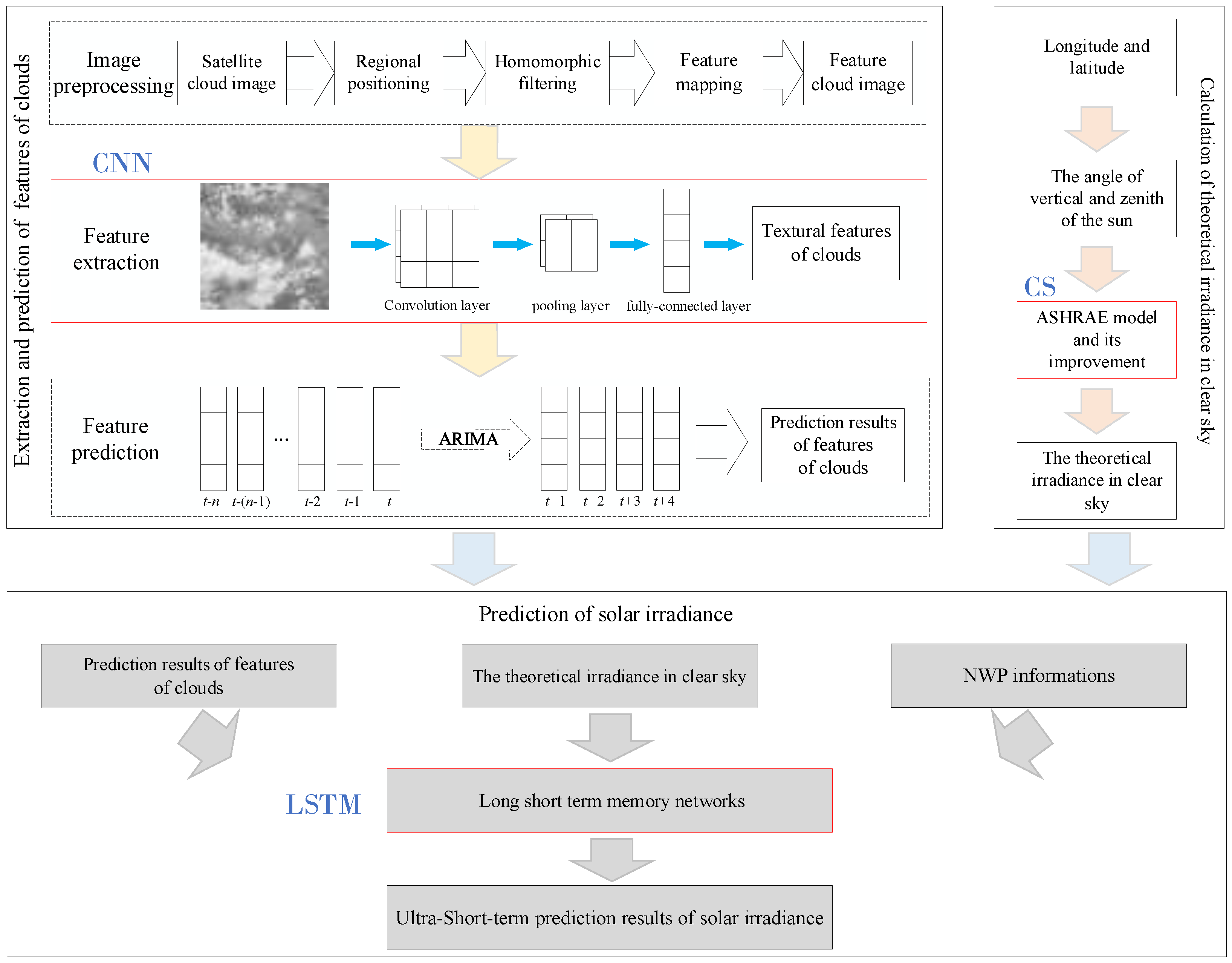
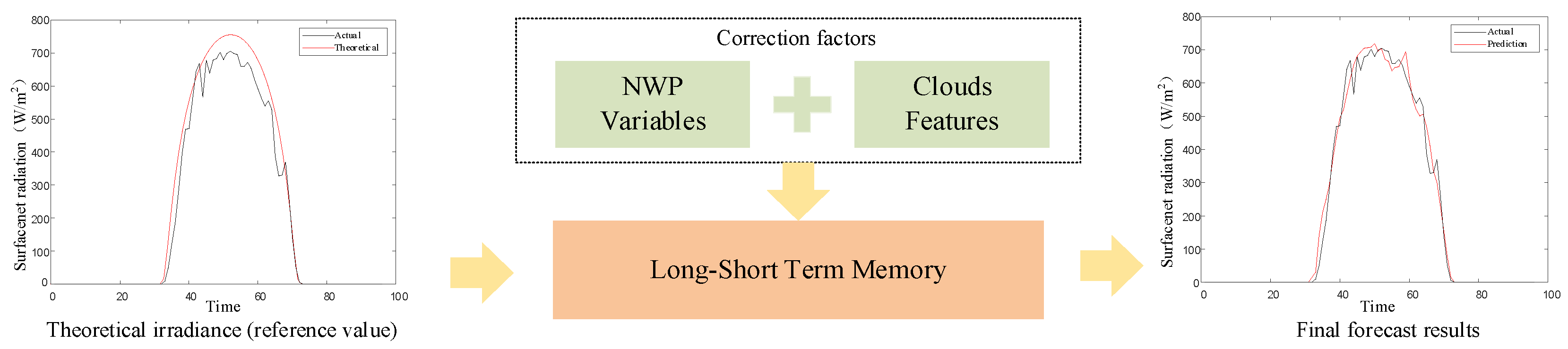
This study proposes an ultra-short-term solar irradiance prediction scheme based on satellite cloud images and a clear sky model. The integrated framework of the scheme is shown in Figure 1. The specific modelling steps are as follows:
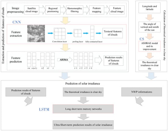
Figure 1.
Integrated framework of the proposed scheme.
- Extraction and prediction of textural features of clouds: First, the textural details of a satellite cloud image were enhanced using homomorphic filtering. Then, a feature mapping model was established for the satellite cloud image to eliminate the difference in diurnal radiation caused by Earth’s movement. Furthermore, a CNN model based on an image textural convolution kernel was established to extract the textural features of clouds. Finally, an autoregressive integrated moving average (ARIMA) model was established to predict the textural features of clouds over the next 1–4 h.
- Calculation of the theoretical irradiance in a clear sky (CS): First, the solar vertical angle, altitude angle, azimuth, zenith angle, and other information were determined through the longitude and latitude of the station. Thereafter, the information was input into the ASHRAE model to obtain the theoretical irradiance of the station in a clear sky. Finally, the theoretical irradiance was compared with the actual irradiance, and the parameters of the ASHRAE model were improved by the least squares method to obtain the theoretical irradiance that conforms to the actual irradiance change trend of the station.
- Prediction of solar irradiance: The LSTM model was established to predict the solar irradiance up to 4h ahead using the textural features of clouds, theoretical irradiance in a clear sky, and NWP information, and the prediction results were evaluated.
3. Methodology
In this section, we introduce our novel solar irradiance forecasting framework, which is based on three main models: (1) a CNN with a textural convolution kernel to extract the textural features of clouds, (2) an improved clear sky model to calculate the theoretical irradiance, and (3) an LSTM to predict solar irradiance. The details of these models will be provided in the following sections.
3.1. CNN with Textural Convolution Kernel
We first utilise the CNN with the textural convolution kernel as a powerful feature extraction tool for clouds. The aim of using the textural convolution kernel is to obtain textural features of clouds. Texture is a feature that reflects the homogeneous phenomenon in an image [40], which reflects the arrangement attribute of the object surface with a slow or periodic change and is the fundamental attribute for verifying the difference between objects. Therefore, the textural features of clouds can express different cloud types, and they have more advantages in PV power prediction compared to cover features of clouds.
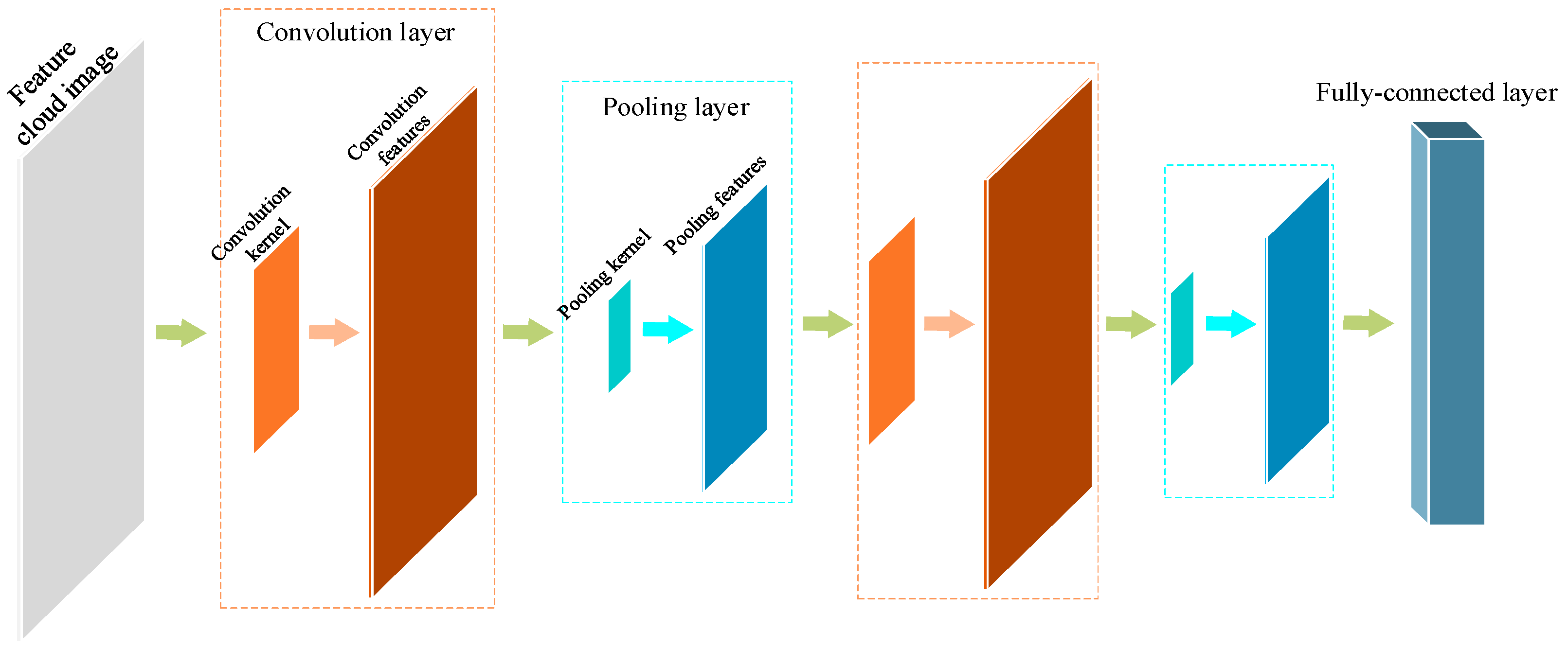
Based on image textural expression, we propose a textural convolution kernel and design a CNN model to extract textural features of clouds. The model includes two convolution layers, pooling layers, and a fully connected layer. The structure of the model is presented in Figure 2.
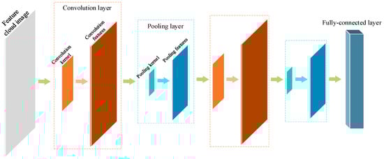
Figure 2.
Structure diagram of the CNN.
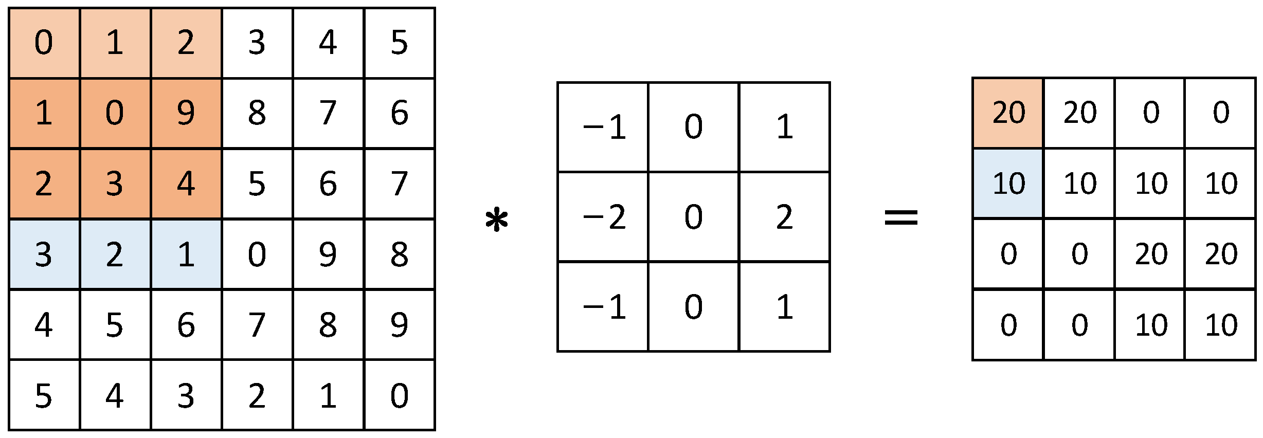
The convolution layer is the core unit of the CNN, which performs convolution operations on images using a convolution kernel. As shown in Figure 3, when performing the convolution operation, the convolution kernel traverses the entire image, calculates the dot product between the pixels in the region and convolution kernel, and changes the calculation results into the characteristic matrix in turn.
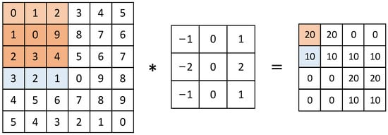
Figure 3.
Rules of convolution operation.
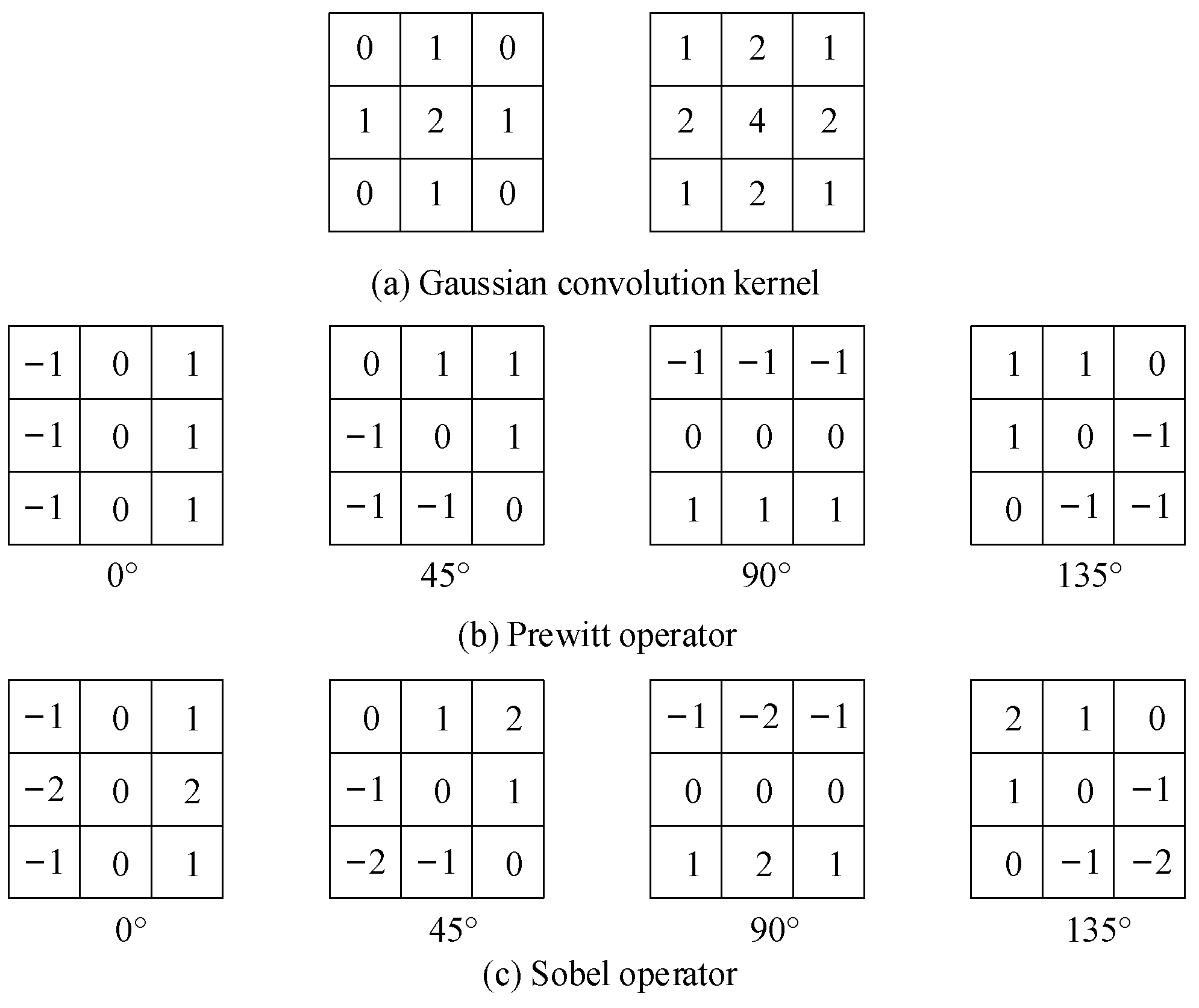
Different convolution kernels and input images were convoluted to obtain different feature matrices. Different features can be extracted by designing different convolutional kernel sizes and values. Common convolution kernels include the Gaussian convolution kernel [41], Prewitt operator [42,43], and Sobel operator [44,45], as illustrated in Figure 4. The Gaussian convolution kernel has smoothing and broadening effects and is mainly used for image filtering and feature enhancement. The Prewitt operator is a differential operator for image edge detection, and its principle is to use the difference generated by the grey value of pixels in a specific area for edge detection. The Sobel operator can not only detect the edge of the image through first-order differential calculation but also obtain the one-order gradient of the image. Prewitt and Sobel operators are the most common convolution kernels in CNN models and are often used for image edge feature extraction in the field of target detection and image classification, which are different from the textural features that this study aims to extract in order to distinguish cloud types.
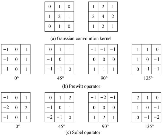
Figure 4.
Common convolution kernels.
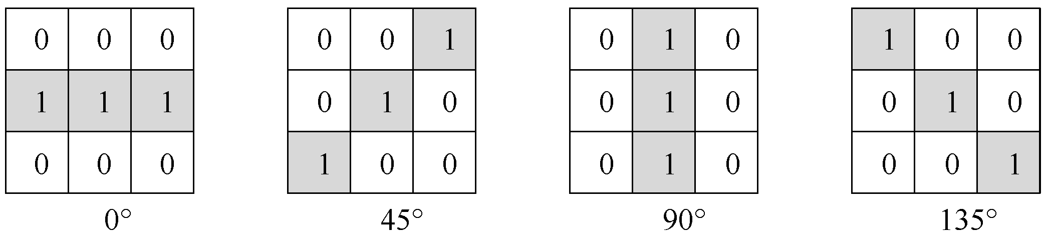
Accordingly, a novel textural convolution kernel of the CNN is proposed that simulates the calculation method of the Grey-level co-occurrence matrix (GLCM) and is used to extract textural features of images in a specified gradient direction, as shown in Figure 5.
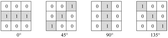
Figure 5.
The proposed textural convolution kernel.
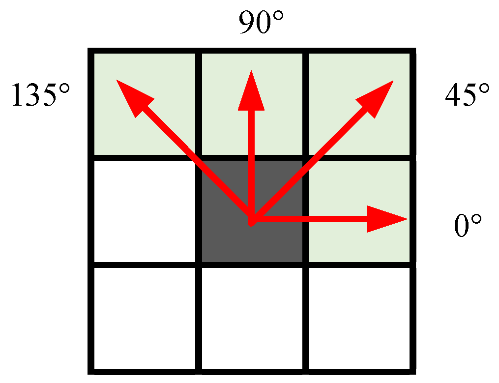
GLCM [46] is a method for the statistical analysis of the spatial characteristics of image pixels, which is widely used in image texture analysis. It describes the textural information of an image in different gradient directions by extracting the intensity relationship between adjacent pixels in different gradient directions, as shown in Figure 6.

Figure 6.
Gradient direction of GLCM.
An image is converted into a matrix that responds to pixel values within a specified distance. This process calculates the frequency of occurrence of pixel pairs at varying distances and directions, which are defined as horizontal, vertical, and diagonal orientations [46].
where .
where is the GLCM of distance d and angle . I(x, y) and I(m, n) are the pixel intensity at position (x, y) and (m, n). and depend on direction and are evaluated using Table 1.

Table 1.
and correspond to direction in GLCM.
Figure 7 shows an example of GLCM calculation where the first matrix is a 5 × 5 image with eight grey levels, 1–8, and the second matrix is the GLCM. Consider a pair of pixels (2, 3) with d = 1 and marked in red circles, two times in the image, which sets the GLCM value as two for this pair. Other pairs are measured similarly too.
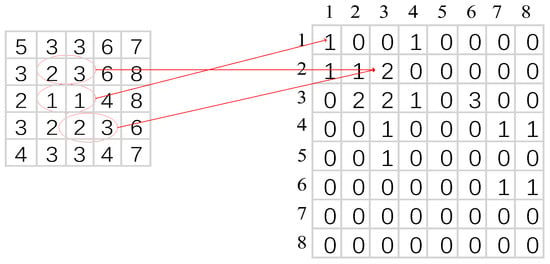
Figure 7.
An example of a GLCM calculation (d = 1, θ = 0°).
The textural convolution kernel sets a valid value of 1 in the direction of the gradient, while the value is set to 0 in other positions. According to the convolution algorithm, when using the textural convolution kernel for convolution operation and feature extraction, the result is the superposition of pixel values in the current gradient direction, and the extracted features are more in line with the definition of textural features. When using a CNN for featural extraction of satellite cloud images, textural convolution kernels slide to collect textural features on different regions of the image, and the similarities and differences in textural features between adjacent regions can also be further reflected. Therefore, the textural convolution kernels and CNNs proposed in this study can extract textural features that describe the type of clouds.
In the study of image texture, the textural gradient directions are generally set to 0°, 45°, 90°, and 135°, so the textural convolution kernel also sets the four gradient directions. In CNNs, the size of the convolution kernel is usually set to squares of 3 × 3, 5 × 5, or 7 × 7. They were considered, and a detailed comparison was made in the solar irradiance prediction example in Section 5.2.
3.2. Improved Clear Sky Model
The second step obtains the theoretical irradiance in a clear sky and supplies a reference value of irradiance in the places of distributed PVs, fundamental data used for solar irradiance forecasting. The ASHRAE model is a general prediction model of surface irradiance in clear skies developed by the American Society of Heating, Refrigerating, and Air-Conditioning Engineers based on research by Threlkeld and Jordan [13]. The ASHRAE model assumes that the weather is clear (there are no or almost no clouds in the sky, and the air quality is very good) and calculates the surface irradiance through historical empirical data and physical formulas. Therefore, the calculation result is the theoretical irradiance that can be received on the ground in a clear sky.
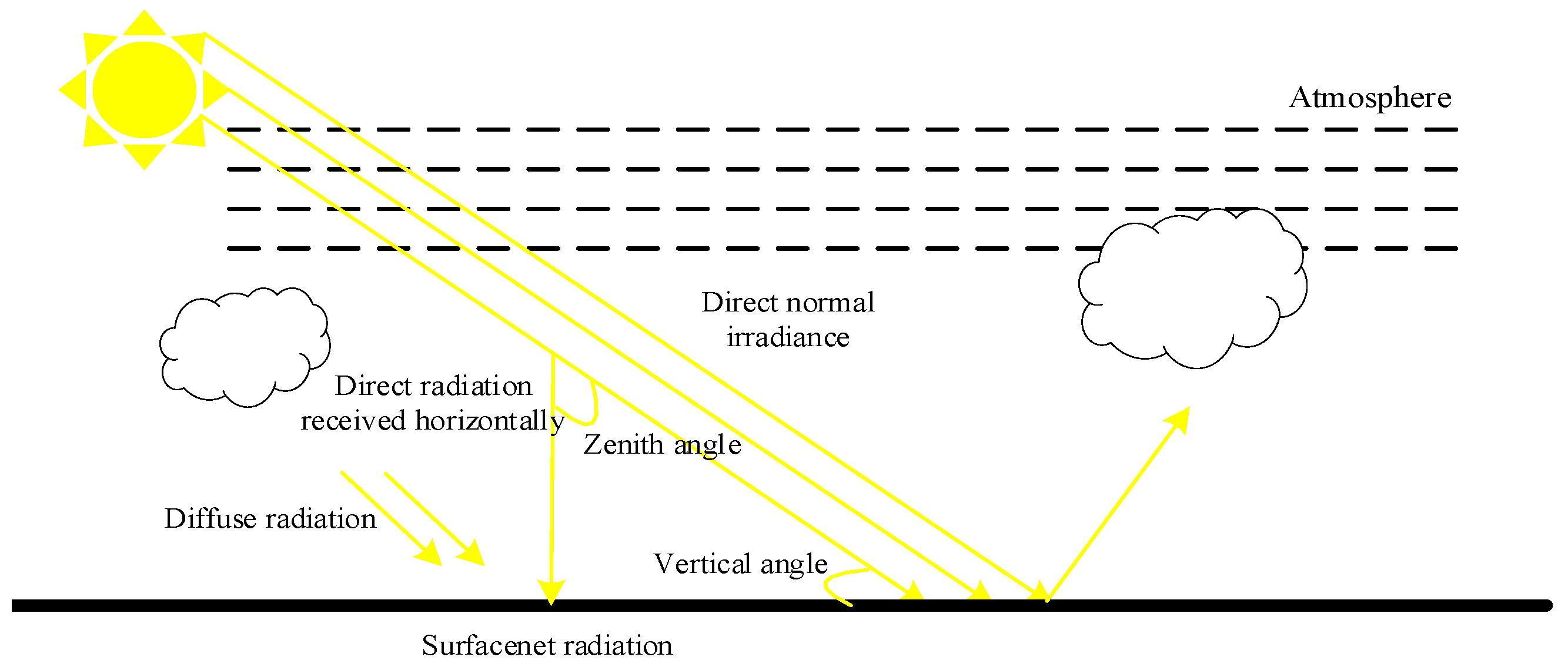
The solar irradiance received by the ground is shown in Figure 8. According to the ASHRAE model, the direct normal irradiance Ib reaching the earth’s surface can be expressed as
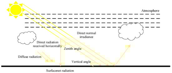
Figure 8.
Solar irradiance relationship.
The diffuse radiation Id can be approximately expressed as
The calculation formula of Surfacenet radiation I is
In Equations (3)–(5), A is the radiation flux outside the atmosphere, k is a dimensionless factor representing the depth of light, θz is the zenith angle of the sun, and n is the number of days from 1 January. A and k are functions considering the distance between the sun and the Earth’s revolution, which are obtained from the iterative regression of the actual irradiance and can be expressed as follows:
In Equations (6) and (7), a1, a2, a3, k1, k2, and k3 are the coefficients obtained via iterative regression.
The ASHRAE model does not consider the surface and climatic characteristics. To adapt to the climatic and geographical conditions of the station to be measured, it is necessary to change the parameters of the ASHRAE model to determine the change trend in irradiance that most conforms to the station. The ASHRAE model primarily relies on the sine function in A and k to reflect the annual and diurnal changes in solar irradiance [13]. A mainly affects the annual solar irradiance change, and k mainly affects the change in solar irradiance within the day. a1 mainly affects the annual solar irradiance amplitude, a2 mainly affects the annual variation in solar irradiance, and a3 mainly affects the variation trend in solar irradiance in the year. k1 mainly affects the amplitude of intraday solar irradiance, whereas k2 and k3 have weak effects on the changes in annual and diurnal solar irradiance.
In this study, the parameters of the ASHRAE model are fitted using the ordinary least squares model, and the specific steps are as follows:
- The sine function in A is a function of the day. The function y = a2sin(2π(n−a3)/365), with a3 as the variable, is defined as the annual solar irradiance change curve. a2 and a3 are fitted by the least squares method according to the annual change in the actual irradiance amplitude of the station, and the parameters a2 and a3 are adjusted to make the ASHRAE model conform to the annual solar irradiance change trend of the station.
- The actual irradiance is backfilled according to the function y = a2sin(2π(n−a3)/365) of the determined parameters; therefore, the variation in solar irradiance in the year is shielded, and the rest is the basic amplitude of solar irradiance in the year. Parameter a1 in A is solved according to Equations (3) and (6).
- According to the change in solar irradiance in the day, the parameter k1 in k is improved using the least squares model.
- According to the prediction results of annual solar irradiance, the parameters k2 and k3 are improved using the least squares model.
3.3. LSTM Model
A long short-term memory network (LSTM) is a kind of time recurrent neural network, which is used to solve the long-term dependence problem of RNN. It saves information for later use so as to prevent earlier information from disappearing gradually during processing. It controls the state of memory cells through a mechanism called a ‘gate’. Figure 9 shows a cycle unit structure [47].
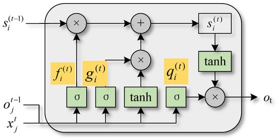
Figure 9.
A cycle unit structure diagram of LSTM.
The information transmission process can be expressed as Equations (8)–(12).
where and are bipolar sigmoid activation functions and hyperbolic tangent activation functions, respectively. indicates the forgetting gate output value of the ith unit at the current time, indicates the value of the input gate at the current time, and indicates the value of the output gate. represents input vector of the current moment, and is its number. includes all the outputs of a cell at the previous moment, which can be regarded as the current hidden layer vector. represent input bias, input weight, and cycle weight of the cell forgetting gate; represent input bias, input weight, and cycle weight of the input gate; and are input bias, input weight, and cycle weight of the output gate. indicates the value of the current time of the state unit. The weight of the state unit self-cycle is the output of the forgetting gate .
The solar irradiance obtained from Section 3.2 is the theoretical irradiance that can be received by the ground under clear sky conditions (good weather, cloudless sky). Then, taking theoretical irradiance as the reference value, LSTM model training is used to fit the attenuation effect of meteorological factors (NWP variables and cloud features) on theoretical irradiance to obtain the prediction model of solar irradiance, as shown in Figure 10.
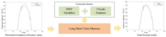
Figure 10.
Solar irradiance prediction model.
4. Case Study
4.1. Data Description and Preprocessing
This study used the historical data of the station (in Wuwei, Gansu Province, China) from 20 September 2017 to 29 December 2018 and selected a relatively complete 113-day period to validate the proposed method.
The satellite cloud image was a free infrared cloud image provided by the FY-2E satellite of the China Satellite Meteorological Center. The longitude and latitude of the station are 102.07° E and 38.35° N; therefore, the range of the satellite cloud images selected in this study is 101°–103° E and 37.5°–39.5° N.
To describe the features of clouds more accurately, the regional cloud image was transformed from the spatial domain to the frequency domain by Fourier transform, and then the textural details of the cloud image were enhanced by homomorphic filtering.
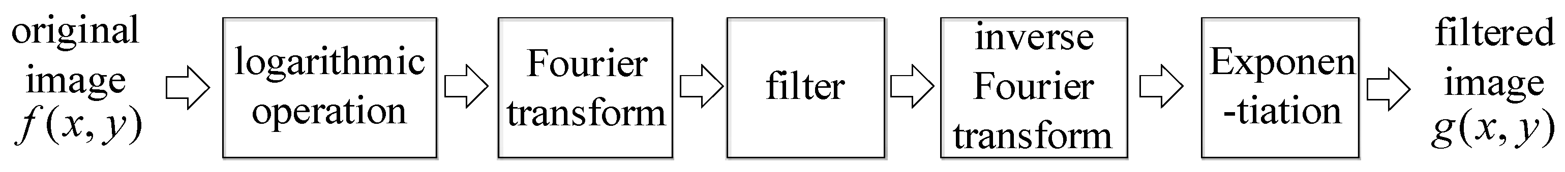
Homomorphic filtering is a method that simultaneously compresses the image brightness range and enhances the image contrast in the frequency domain, which can simultaneously increase the contrast, as well as standardise the brightness to make the illumination of the image more uniform, and achieve enhancement of image details in dark areas without loss of the image details in bright areas by eliminating the multiplicative noises in the image [48]; a specific flowchart is shown in Figure 11.

Figure 11.
Flow chart for homomorphic filtering.
The image f(x, y) composed of pixel points (x, y) usually consists of two parts, the irradiation function i(x, y) and the reflection function r(x, y), as shown in Equation (13). i(x, y) describes the illuminated portion of the image, which is in the low frequency, and r(x, y) describes the texture details of the image, which is in the high frequency.
The two parts of the image multiply together to represent the image and cannot be processed separately, while the homomorphic filtering uses a logarithmic function to transform the two parts from multiplication to addition, as shown in Equation (14).
The image F(u, v) and the irradiation function I(u, v) and reflection function R(u, v) in the frequency domain are obtained by Fourier transform to the frequency domain, as shown in Equation (15).
The image is enhanced using the filter function H(u, v) as shown in Equation (16).
Since the reflection function is concentrated in the high-frequency band, H(u, v) is chosen as the high-pass filtering function in order to obtain more texture details in the image, and its expression is shown in Equation (17).
where and are the high-frequency gain value and low-frequency gain value, respectively (selecting > 1 and < 1 can achieve the purpose of attenuating the low frequency and enhancing the high frequency); c is the sharpness of the slope of the control function; and D(u, v) and D0 denote the distance from the centre of the frequency and the cutoff frequency, respectively.
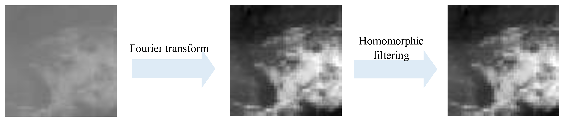
Considering the cloud image at 00:30 on 27 September 2017 as an example, the results after homomorphic filtering are shown in Figure 12. Compared with the previous images, we can see that the cloud characteristics are better and more accurate after homomorphic filtering.
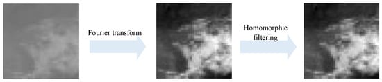
Figure 12.
Homomorphic filtering processing result.
4.2. Determination of the Input Variables
The choice of suitable input variables is crucial for determining the forecasting accuracy of artificial intelligence models. Insufficient input data can lead to poor forecasting performance, while including too many variables can cause the issue of dimensionality, which may result in longer computation times and reduced model efficiency [20].
The input variables for the ultra-short-term solar irradiance prediction model is divided into three parts: the first part is the textural features of clouds, which is extracted from the CNN with textural convolution kernel and predicted using an ARMA model in the next 1–4 h, the second part is the theoretical irradiance in clear sky calculated by the improved ASHRAE model, and the third part of inputs are NWP variables that are strongly related to solar irradiance, including temperature, humidity, precipitation, shortwave radiation, and sensible heat flux. The correlation coefficients, which are calculated from Pearson’s correlations, are presented in Table 2.
Table 2.
Correlation coefficient between solar irradiance and variables in NWP.
The satellite cloud image enhanced by homomorphic filtering is feature-mapped to obtain the feature cloud image, and then the textural features of the cloud are extracted from the feature cloud image based on the CNN with TCK.
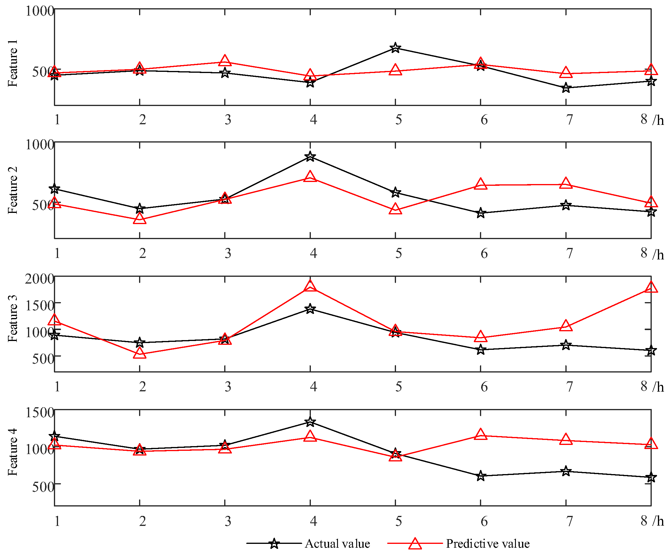
Based on the extracted cloud textural features at historical times, ARIMA models are established to predict future cloud textural features. Firstly, a stationarity test on the cloud textural features is performed. If it is a non-stationary time series, differential processing is performed until it becomes a stationary sequence. The number of differences is the order of difference d in the ARIMA (p, d, q) model. Then, based on the autocorrelation function (ACF) and partial autocorrelation function (PACF) of the feature sequence, the AIC and SC function values are calculated to determine the optimal autoregressive term p and moving average term q. In the ARIMA model, p indicates that the future time value is related to the previous p time values, and q indicates that the future time noise is related to the previous q time noise. Therefore, the order of the ARIMA model is determined based on the values of p and q. According to the above steps, the ARIMA time-series prediction model for cloud texture features was trained and debugged, and the parameters of the ARIMA model were finally determined to be p = 7, d = 1, and q = 3. The prediction results of each textural feature as the prediction time increases are shown in Figure 13. It can be seen that the prediction results are very good within 1–4 h, which can fit the changes in cloud cluster characteristics in a short period of time. The prediction effect worsens between 5 and 8 h. And the Mean Absolute Percentage Error (MAPE) is calculated as shown in Table 3 below, from which it can be seen that the prediction errors of all four features in 1–4 h are relatively small, and the prediction errors in 5–8 h are larger. Based on the prediction effect of cloud textural features, it is shown that the predicted cloud textural features are applicable to solar irradiance prediction up to 4 h ahead.

Figure 13.
Results of clouds textural features for different hours ahead forecasting.
Table 3.
Errors in cloud texture characterisation results for different hours ahead forecasting.
The time resolution of the satellite cloud image used in this study was 1 h, while the time resolution of the predicted power of the photovoltaic power station was generally 15 min. The textural features of clouds at 15 min intervals were obtained by linear interpolation.
Based on the correction steps of the clear sky model described in Section 3.2, we set the parameters of formulas A and k in Equations (6) and (7) as follows.
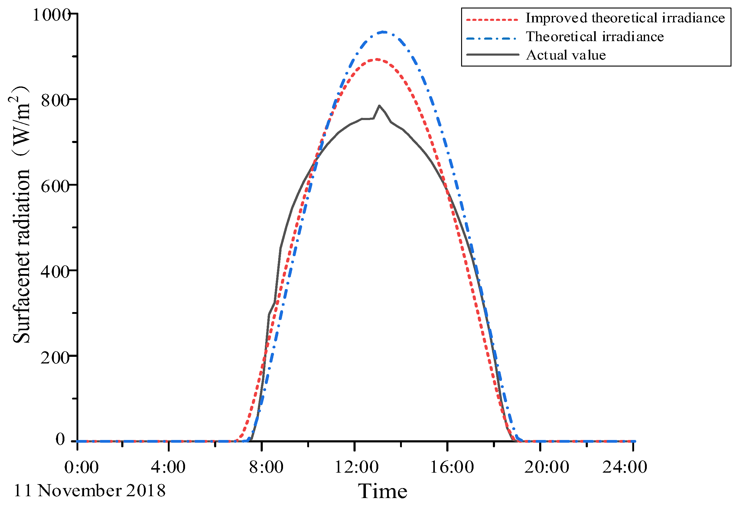
The results of the theoretical irradiance in the clear sky calculated based on the improved ASHRAE model are shown in Figure 14. The error calculations are shown in Table 4 below. It can be seen that the theoretical irradiance obtained from the improved clear-sky model is more consistent with the trend in actual irradiance changes and has a smaller error margin. However, the ASHRAE model does not consider complex weather changes, and the prediction result is the theoretical value under clear sky conditions. Although the change trend in solar irradiance can be fitted, the predicted value is higher than the actual value. Therefore, it is necessary to amend the theoretical irradiance in the clear sky model with other weather information.
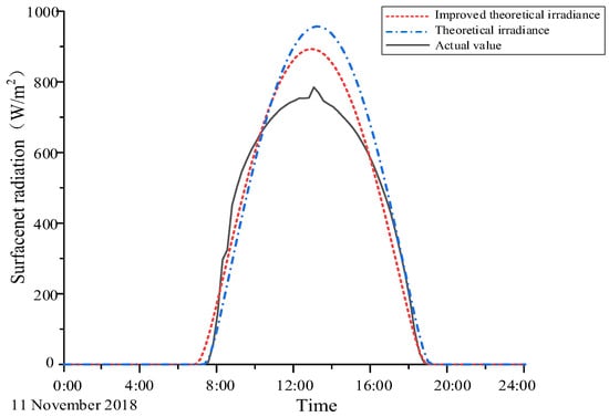
Figure 14.
Comparison of theoretical irradiance with actual values.
Table 4.
Comparison of errors between theoretical irradiance and actual values.
4.3. Compared Models
To highlight the effectiveness of the proposed integrated framework, comprehensive comparisons are made in this study by constructing the other models. The experiments are divided into four groups: the first group is the NWP result, which is represented by the WRF-Solar model; the second group contains three common models, which are the ANN, SVR, and LSTM prediction results; the third group of experiments are the results of the partially integrated framework, CNN-LSTM and CS-LSTM; and the fourth group are the results of three feature extraction methods—PO-CS-LSTM, SO-CS-LSTM, and TCK-CS-LSTM—where PO represents Prewitt operator and SO represents Sobel operator.
The NWP and CS models display the rough solar radiation without any machine learning process to show the necessity of machine learning. The performance of the two popular machine learning methods, including ANN and SVR, is evaluated to highlight the performance of the standalone LSTM model. The partially integrated models CNN-LSTM and CS-LSTM are constructed to demonstrate the effectiveness of cloud feature extraction with CNN and the CS calculation in forecasting solar radiation. The feature extraction-based models including PO-CS-LSTM and SO-CS-LSTM are also constructed to compare with the proposed TCK-CS-LSTM model to further validate the effectiveness of the TCK method in extracting textural features of clouds and improving the solar radiation forecasting.
4.4. Performance Criteria
Three types of widely used metrics were used to evaluate model performance. The mean absolute error (MAE), the root mean square error (RMSE), and the correlation coefficient (R2) were described as follows.
where yi and are the actual and forecasted solar radiation at point i, respectively; n represents the total number of forecasting points.
5. Results and Discussion
The nine models constructed in this study are applied to the solar radiation datasets for forecasting. The model performances are evaluated by three statistical measures including RMSE, MAE, and R2. This section compares the results of the proposed TCK-CS-LSTM model with the other contrast methods including NWP, ANN, SVR, LSTM, CS-LSTM, CNN-LSTM, PO-CS-LSTM, and SO-CS-LSTM. It can be categorised into four groups. The first group includes the NWP model, which provides predictions without machine learning. The second group includes three traditional models—ANN, SVR, and LSTM—to highlight the performance of LSTM. The third group consists of partially integrated models CNN-LSTM and CS-LSTM, which combine CNN extraction of cloud features and CS computation of forecast solar radiation to improve prediction. The last group compares three cloud models based on feature extraction, the PO-CS-LSTM, the SO-CS-LSTM, and the proposed TCK-CS-LSTM, where PO and SO stand for Prewitt operator and Sobel operator, respectively, and TCK is the texture convolution kernel proposed in this paper.
5.1. Comparison of Prediction Results Using Different Input Variables
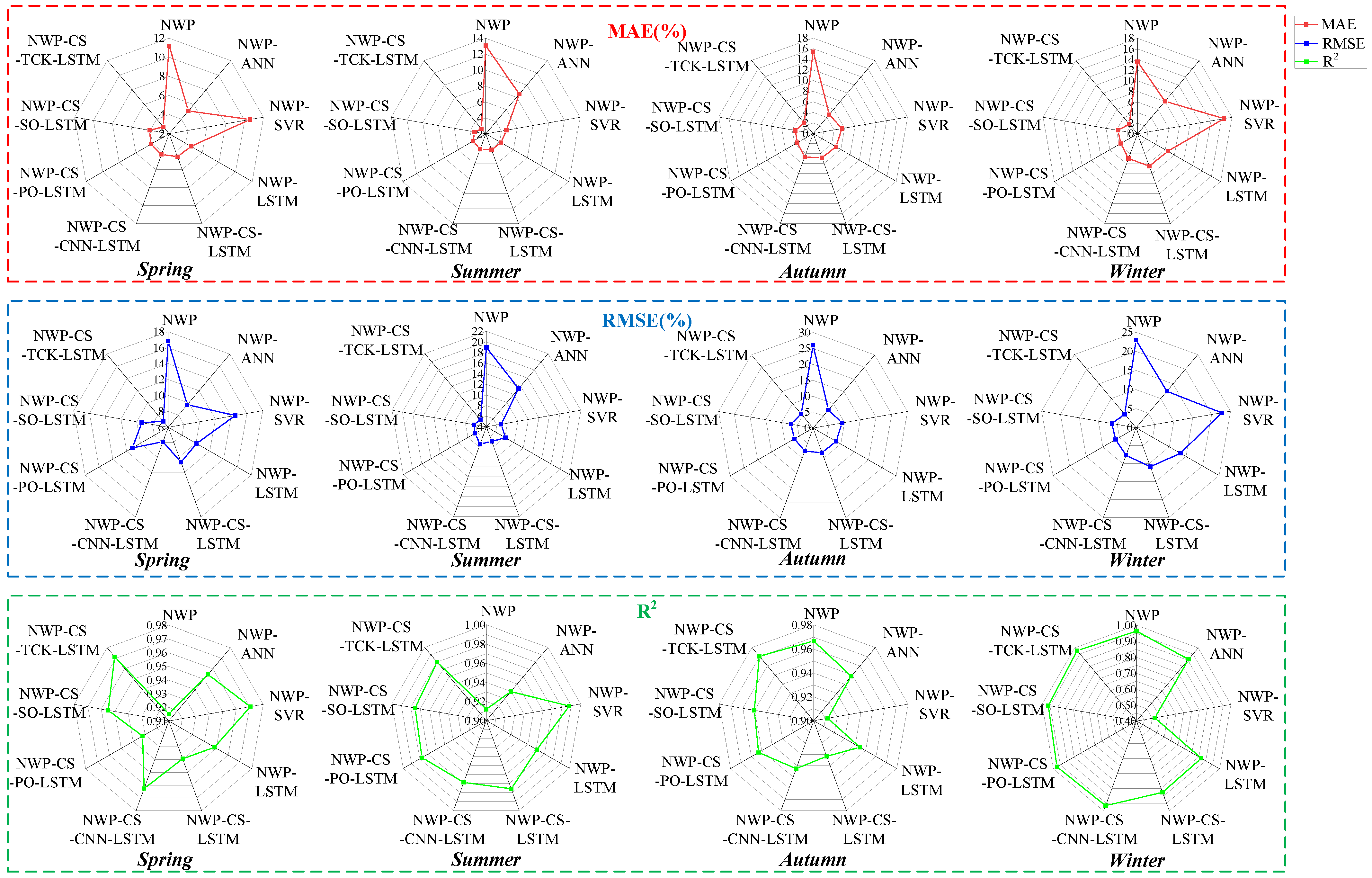
The solar radiation forecasting results using different input variables for the datasets are firstly compared and analysed in this section. The values of the three statistical measures including RMSE, MAE, and R2 are listed in Table 5 for the proposed and the contrast models. To exhibit the error measures more intuitively, the RMSE, MAE, and R values of the nine models for the four datasets are illustrated using radar plots in Figure 15. The experimental results in Table 5 demonstrate the solar irradiance prediction performance of different models under different seasons. By comparing the performance metrics such as MAE, RMSE, and R2, it can be seen that the proposed TCK-CS-LSTM model exhibits optimal prediction performance in all seasons.
Table 5.
Solar irradiance prediction results of different models under different seasons.
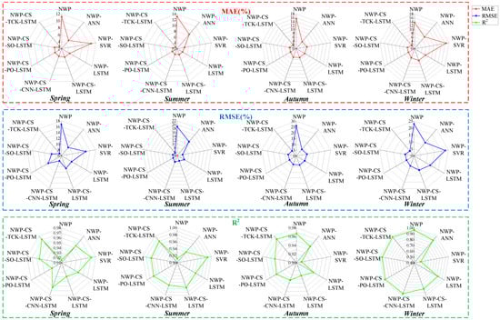
Figure 15.
Solar irradiance prediction performance of different models under different seasons.
- NWP lacks sufficient accuracy in predicting solar radiation; thus, relying only on numerical weather prediction for solar radiation prediction is limiting, and the introduction of machine learning methods is necessary.
- Comparing ANN, SVR, and LSTM models, in general, LSTM has a more balanced performance in different seasons, demonstrating its advantages in dealing with complex nonlinear relationships. In contrast, ANN, although it performs well in some cases, is not as robust as LSTM in some seasons. The SVR model performs well under specific conditions, but its performance fluctuates greatly when dealing with complex weather changes, and its performance is obviously not as stable as that of LSTM. Therefore, LSTM is more adaptable and stable in dealing with diverse weather conditions.
- Comparison results between the partially integrated models (CNN-LSTM and CS-LSTM) and the comprehensive integrated models (PO-CS-LSTM, SO-CS-LSTM, and TCK-CS-LSTM) show that the comprehensive integrated models exhibit superior performance in solar radiation prediction. The partially integrated model significantly improves the prediction accuracy by combining the results of cloud features and clear-sky irradiance through the LSTM model, respectively. However, the comprehensive integrated model is further optimised on this basis by combining the calculated results of cloud features and clear-sky irradiance, which significantly improves the prediction accuracy and stability of the model.
- The comparison between the integrated models shows that the TCK-CS-LSTM model outperforms PO-CS-LSTM and SO-CS-LSTM in all the metrics, indicating that the cloud features extracted by using the texture convolution kernel provide more accurate prediction results than those extracted based on Prewitt and Sobel operators. TCK-CS-LSTM significantly improves the accuracy and stability of cloud feature extraction by introducing the texture convolution kernel, thus demonstrating the optimal prediction performance under complex weather conditions. The texture convolution kernel significantly improves the accuracy and stability of cloud feature extraction and thus demonstrates the optimal prediction performance under complex weather conditions. TCK-CS-LSTM provides the most accurate and reliable solar radiation prediction compared to other models.
5.2. Comparison of Prediction Results with Different Convolution Kernels
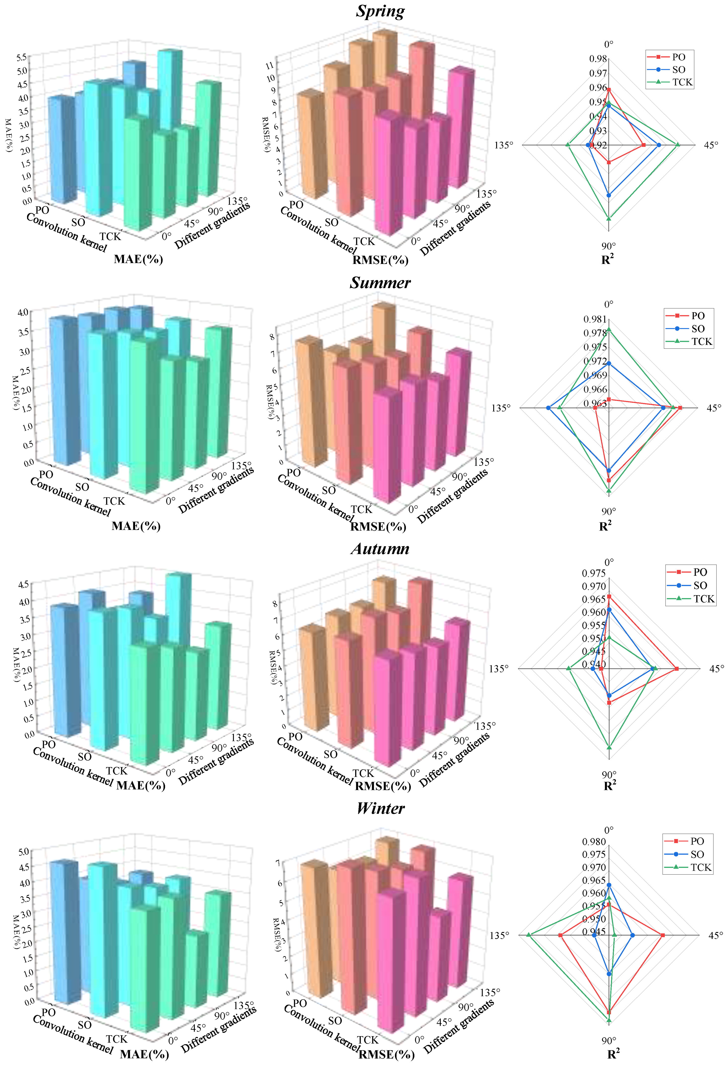
The experimental results in Table 6 and Figure 16 demonstrate the effect of cloud features extracted from four gradient orientations with different convolutional kernels on the solar irradiance prediction accuracy in different seasons. By comparing the performance metrics of MAE, RMSE, and R2, TCK performs much better in all seasons and metrics. In contrast, the Prewitt and Sobel operators perform with less overall accuracy than TCK in MAE and RMSE, although with some stability. This suggests that TCK is able to better extract the cloud texture features, thus providing higher prediction accuracy and stability. Further analysing the effect of cloud mass features extracted by TCK on the prediction results under different gradient orientations, the performance of 90° orientation is particularly outstanding. For example, in spring and winter, the MAE of the 90° direction is as low as 2.95% and 2.41%, respectively, which is more accurate than the results of other directions. The corresponding RMSE and R2 values also indicate that the convolution kernel in the 90° gradient direction is more capable of capturing cloud details and complex features.
Table 6.
Predictions of four gradient directions with different convolution kernels under different seasons.
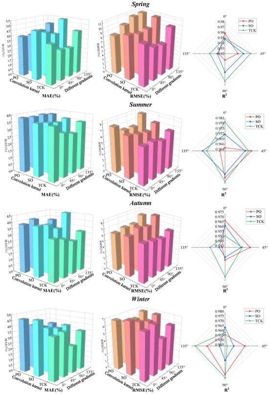
Figure 16.
Comparison of four gradient direction predictions with different convolution kernels under different seasons.
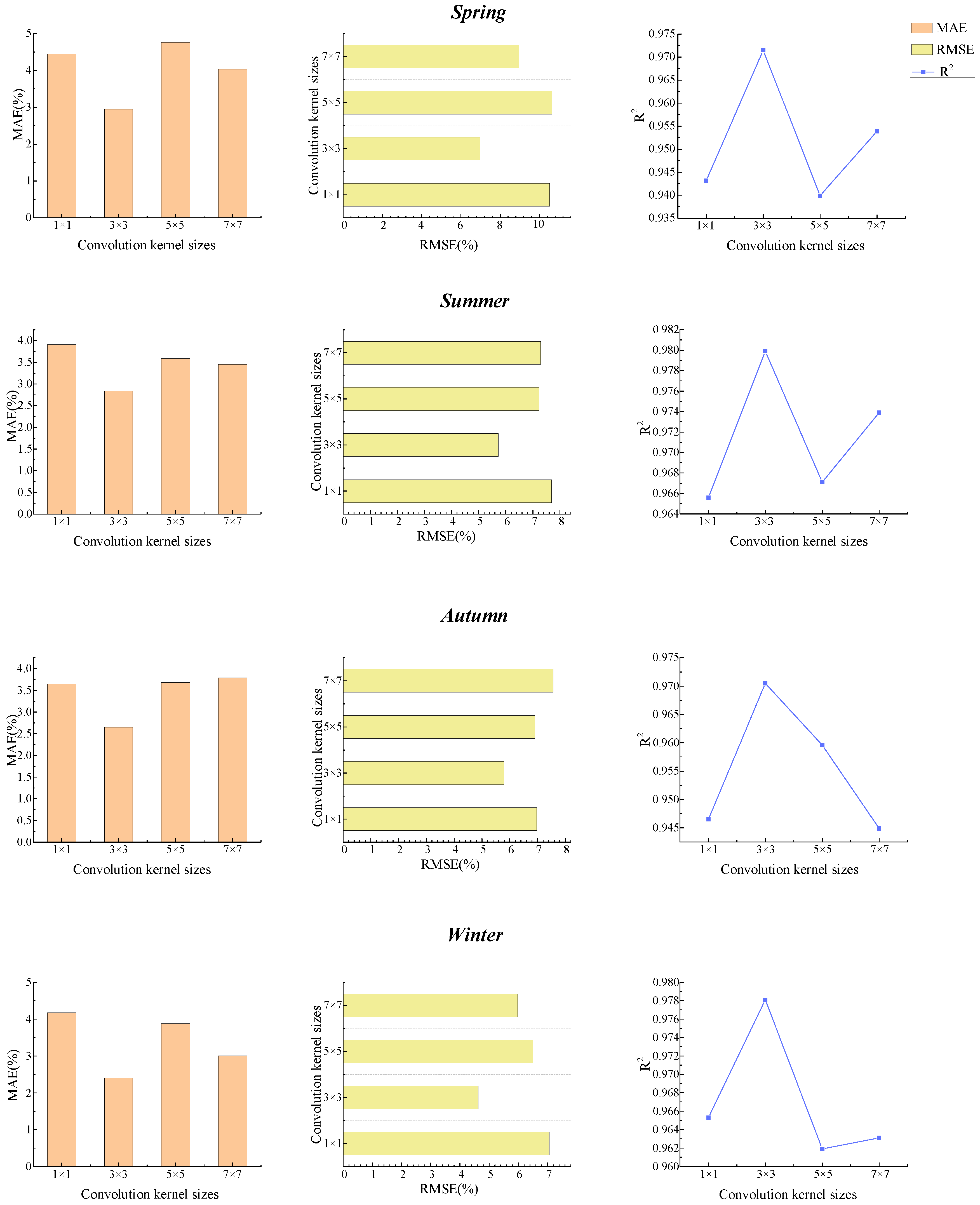
Table 7 and Figure 17 compare the TCK of different sizes, and the 3 × 3 convolutional kernel has the best overall performance, outperforming the other sizes both in terms of prediction error (MAE and RMSE) and model fit (R2). In contrast, the 1 × 1 convolutional kernel is too small to effectively capture complex cloud features, resulting in lower prediction accuracy. 5 × 5 and 7 × 7 convolutional kernels are able to capture more information about image features, but the larger sizes may introduce more noise or redundant information, which in turn reduces the prediction performance of the model.
Table 7.
TCK prediction results for different sizes.
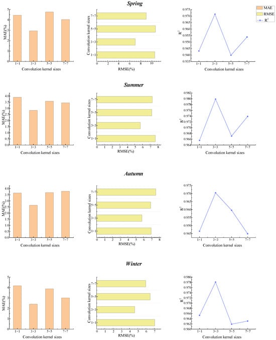
Figure 17.
Comparison of TCK prediction results for different sizes.
5.3. Predicted Results Under Different Weather Conditions
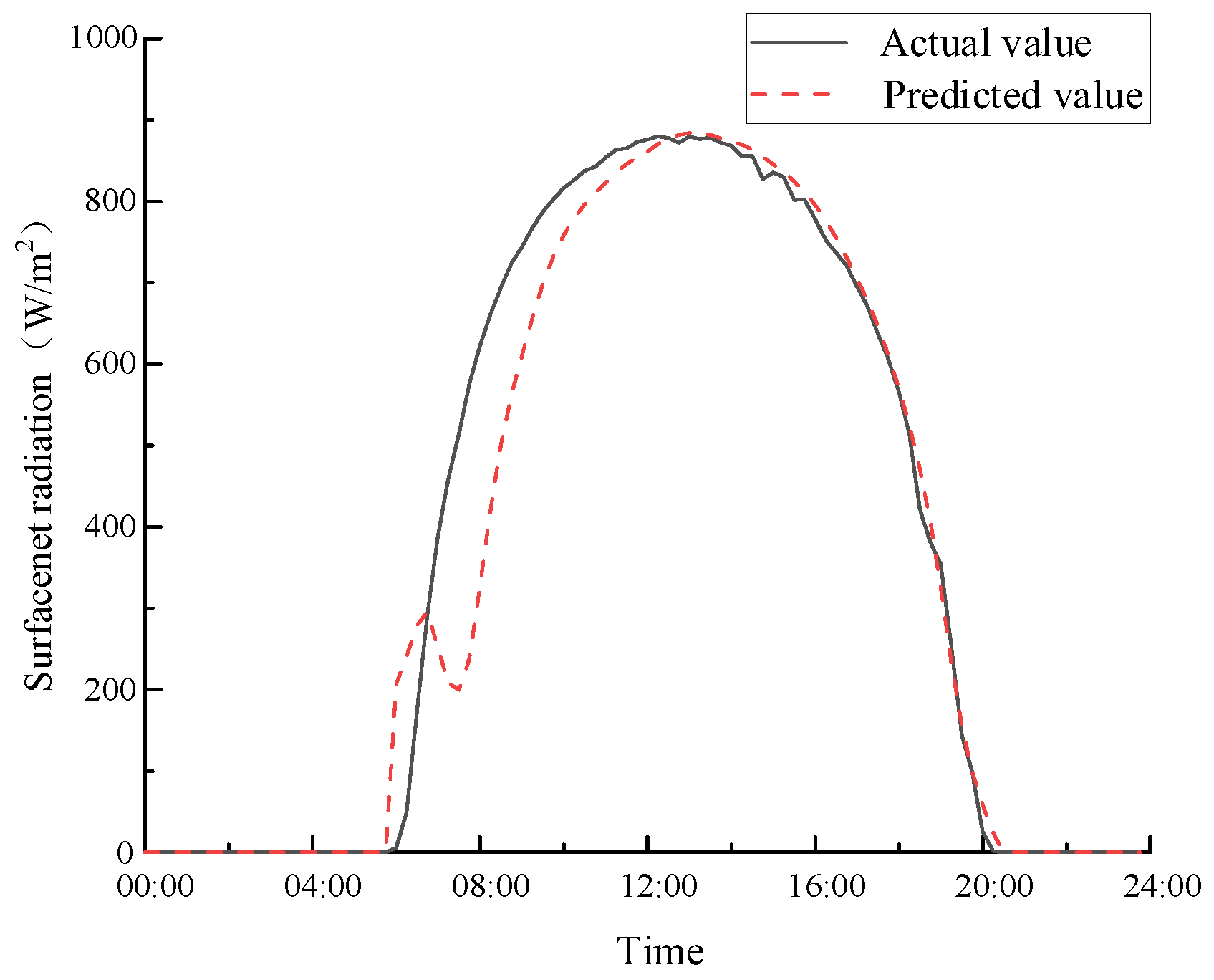
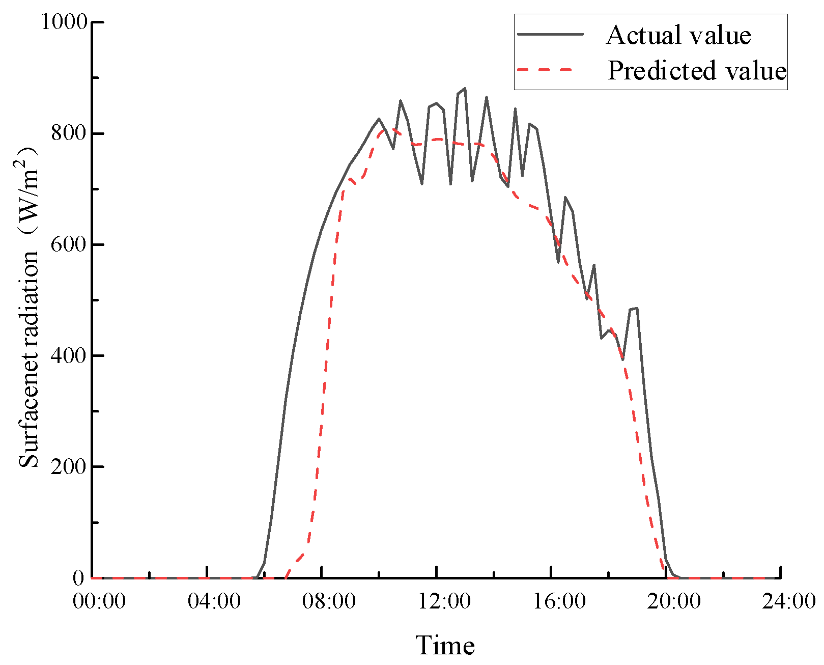
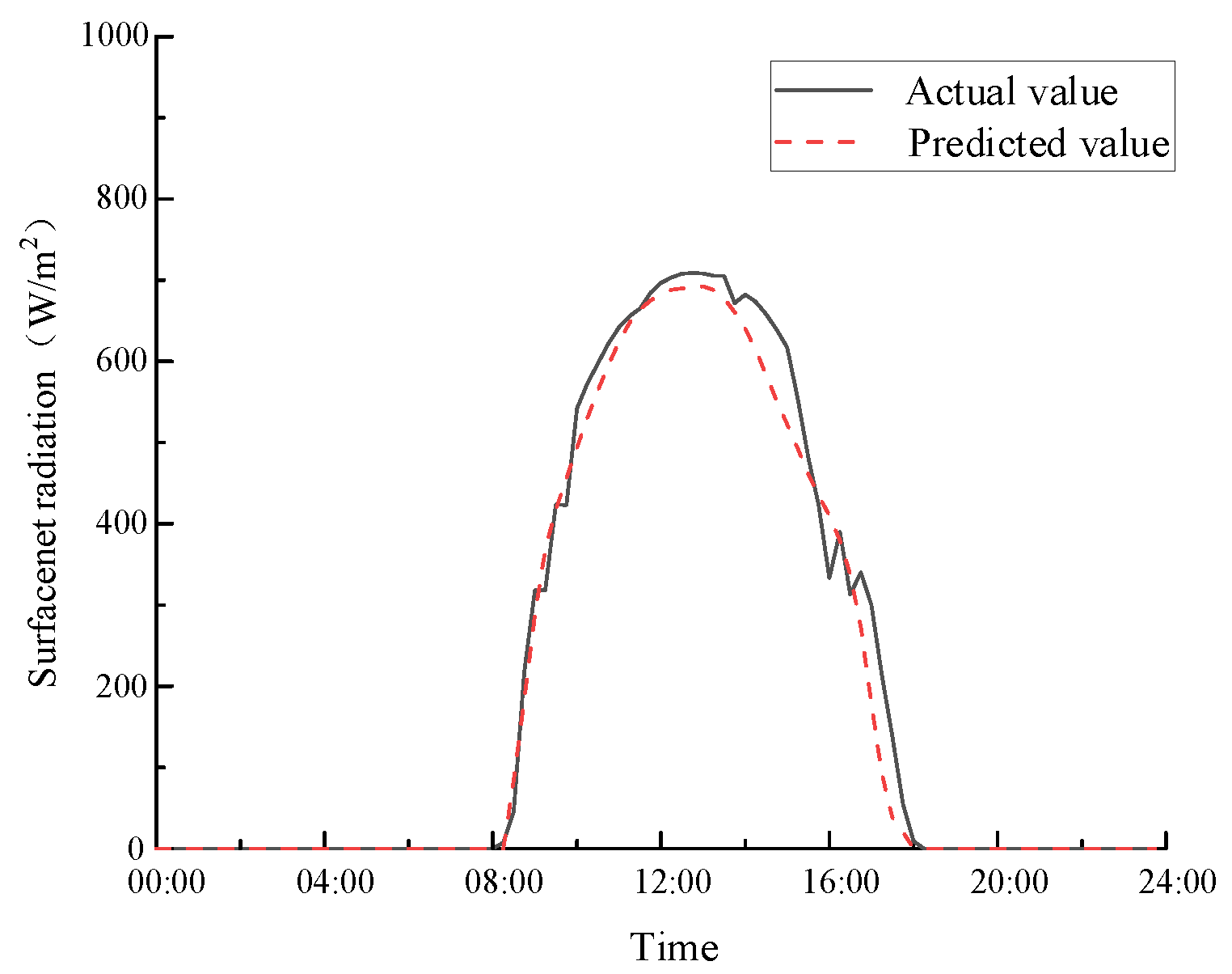
The validity of the prediction under different weather is verified using the TCK-CS-LSTM model with the textured convolution kernel of size 3 × 3 and 90° gradient direction. Figure 18, Figure 19 and Figure 20 below show the prediction results under sunny and cloudy skies, respectively, from which it can be seen that the model is able to make accurate predictions under different weather conditions.
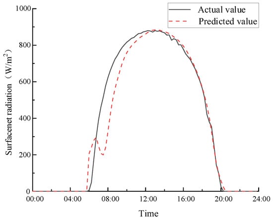
Figure 18.
Predicted results under clear weather.
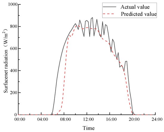
Figure 19.
Predicted results under cloudy weather.
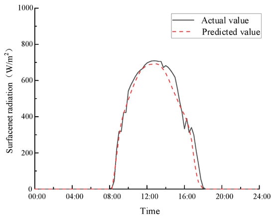
Figure 20.
Predicted results under overcast weather.
6. Conclusions
This study proposes a textural convolution kernel based on a grey-level co-occurrence matrix for extracting the textural features of clouds, constructing and evaluating the performance of an integrated LSTM model based on satellite cloud images and the clear sky model for solar irradiance prediction. According to experimental tests, the main conclusions of this study can be summarised as follows:
- The ultra-short-term prediction accuracy of solar irradiance is improved by introducing textural features of clouds and theoretical irradiance in the clear sky.
- The texture features can better show the shielding effect of clouds on solar radiation and perform better in predicting solar irradiance. Compared with the common Prewitt operator and Sobel operator convolution kernels, the texture convolution kernel proposed in this study has more advantages in displaying the texture features of clouds and predicting the solar irradiance.
- Textural features in the 90° gradient direction are particularly effective, offering the highest prediction accuracy. Additionally, the 3 × 3 convolution kernel size proves to be optimal, providing richer textural details and further improving prediction performance.
Overall, the model proposed in this study shows excellent performance in solar irradiance prediction, providing a more accurate and reliable method compared to traditional methods. As future work, we plan to make an adaptive power prediction model for different photovoltaic panels to convert the predicted solar irradiance into PV power. The research will increase the deployment of PV so as to contribute to achieving a net-zero energy system.
Author Contributions
Conceptualization, L.W. and Y.H.; methodology, L.W.; software, Q.Z.; validation, L.W. and Q.Z.; formal analysis, Q.Z.; investigation, Y.H.; resources, Y.H.; data curation, X.L.; writing—original draft preparation, L.W.; writing—review and editing, X.L.; visualisation, X.L.; supervision, L.W.; project administration, L.W.; funding acquisition, L.W. All authors have read and agreed to the published version of the manuscript.
Funding
This work was supported by the China Scholarship Council (No. 202008110119).
Institutional Review Board Statement
Not applicable.
Informed Consent Statement
Not applicable.
Data Availability Statement
Data are contained within the article.
Conflicts of Interest
The authors declare no conflicts of interest.
References
- Zhang, Q.; Wang, L.; Hao, Y.; Wang, B.; Che, J.; Guo, H. Ultra-short-term Solar Irradiance Prediction of Distributed Photovoltaic Power Stations Based on Satellite Cloud Images and Clear Sky Model. High. Voltage Eng. 2022, 48, 3271–3281. [Google Scholar]
- Eseye, A.T.; Lehtonen, M.; Tukia, T.; Uimonen, S.; Millar, R. Adaptive Predictor Subset Selection Strategy for Enhanced Forecasting of Distributed PV Power Generation. IEEE Access 2019, 7, 90652–90665. [Google Scholar] [CrossRef]
- Nour, A.M.; Hatata, A.Y.; Helal, A.A.; El-Saadawi, M.M. Review on Voltage-Violation Mitigation Techniques of Distribution Networks with Distributed Rooftop PV Systems. IET Gener. Transm. Distrib. 2020, 14, 349–361. [Google Scholar] [CrossRef]
- Zhang, L.; Wang, X.; Wu, H. Ultra-Short-Term Prediction of PV Power Based on FCM and LSTM. Electr. Supply 2023, 40, 10–17. [Google Scholar]
- Ahmed, S.I.; Bhuiyan, K.A.; Rahman, I.; Salehfar, H.; Selvaraj, D.F. Reliability of Regression Based Hybrid Machine Learning Models for the Prediction of Solar Photovoltaics Power Generation. Energy Rep. 2024, 12, 5009–5023. [Google Scholar] [CrossRef]
- Shaohua, H.; Xin, F.; Xiuru, W.; Chenyu, Z.; Fuju, Z.; Jiaming, W. Distributed Photovoltaic Power Output Prediction Based on Satellite Cloud Map Video Frames. Front. Energy Res. 2023, 11, 1247304. [Google Scholar] [CrossRef]
- Ismael, S.M.; Aleem, S.H.A.; Abdelaziz, A.Y.; Zobaa, A.F. State-of-the-Art of Hosting Capacity in Modern Power Systems with Distributed Generation. Renew. Energy 2019, 130, 1002–1020. [Google Scholar] [CrossRef]
- Lu, H.; Chai, Y.; Hao, J.; Chen, X.; Guo, L.; Liu, Y. Network Simplification-Based Cluster Coordinated Optimization Method for Distributed Pvs with Inadequate Measurement. IEEE Access 2020, 8, 65283–65293. [Google Scholar] [CrossRef]
- Zang, H.; Cheng, L.; Ding, T.; Cheung, K.W.; Wang, M.; Wei, Z.; Sun, G. Application of Functional Deep Belief Network for Estimating Daily Global Solar Radiation: A case study in China. Energy 2020, 191, 116502. [Google Scholar] [CrossRef]
- Kabir, E.; Kumar, P.; Kumar, S.; Adelodun, A.A.; Kim, K.H. Solar Energy: Potential and Future Prospects. Renew. Sustain. Energy Rev. 2018, 82, 894–900. [Google Scholar] [CrossRef]
- Yang, D. Choice of Clear-Sky Model in Solar Forecasting. J. Renew. Sustain. Energy 2020, 12, 026101. [Google Scholar] [CrossRef]
- Yao, W.; Xu, C.; Zhao, J.; Wang, X.; Wang, Y.; Li, X.; Cao, J. The Modified ASHRAE Model Based on the Mechanism of Multi-Parameter Coupling. Energy Convers Manag. 2020, 209, 112642. [Google Scholar] [CrossRef]
- Razzak, A.; Uddin, Z.; Iqbal, M.J.; Alam, K. Calculation of Urban Solar Radiation Based on Simulation and Fitting of ASHRAE Model Constants. Arab. J. Geosci. 2022, 15, 451. [Google Scholar] [CrossRef]
- Álvarez, O.H.; Montaño, T.E. The Global Solar Radiation in The Southern Region of Ecuador. Open Access Libr. J. 2019, 6, 1–19. [Google Scholar] [CrossRef]
- Zhong, X.; Kleissl, J. Clear Sky Irradiances Using REST2 and MODIS. Sol. Energy 2015, 116, 144–164. [Google Scholar] [CrossRef]
- Zhang, Y.; Wang, Y. The Prediction of Irradiation Degree of Photovoltaic Power Station Based on Weather Clustering. Sci. Technol. Eng. 2021, 21, 1030–1036. [Google Scholar]
- Linares-Rodriguez, A.; Ruiz-Arias, J.A.; Pozo-Vazquez, D.; Tovar-Pescador, J. An Artificial Neural Network Ensemble Model for Estimating Global Solar Radiation from Meteosat Satellite Images. Energy 2013, 61, 636–645. [Google Scholar] [CrossRef]
- Chen, R.; Gao, S.; Zhao, Y.; Li, D.; Lin, S. A Hybrid Model Based on the Photovoltaic Conversion Model and Artificial Neural Network Model for Short-Term Photovoltaic Power Forecasting. Front. Energy Res. 2024, 12, 1446422. [Google Scholar] [CrossRef]
- Wei, L.; Xv, S.; Li, B. Short-Term Wind Power Prediction Using an Improved Grey Wolf Optimization Algorithm with Back-Propagation Neural Network. Clean. Energy 2022, 6, 288–296. [Google Scholar] [CrossRef]
- Peng, T.; Zhang, C.; Zhou, J.; Nazir, M.S. An Integrated Framework of Bi-Directional Long-Short Term Memory (Bilstm) Based on Sine Cosine Algorithm for Hourly Solar Radiation Forecasting. Energy 2021, 221, 119887. [Google Scholar] [CrossRef]
- Farah, S.; Humaira, N.; Aneela, Z.; Steffen, E. Short-Term Multi-Hour Ahead Country-Wide Wind Power Prediction for Germany Using Gated Recurrent Unit Deep Learning. Renew. Sustain. Energy Rev. 2022, 167, 112700. [Google Scholar] [CrossRef]
- Qu, J.; Qian, Z.; Pei, Y. Day-Ahead Hourly Photovoltaic Power Forecasting Using Attention-Based CNN-LSTM Neural Network Embedded with Multiple Relevant and Target Variables Prediction Pattern. Energy 2021, 232, 120996. [Google Scholar] [CrossRef]
- Kaba, K.; Sarıgül, M.; Avcı, M.; Kandırmaz, H.M. Estimation of Daily Global Solar Radiation Using Deep Learning Model. Energy 2018, 162, 126–135. [Google Scholar] [CrossRef]
- Si, Z.; Yang, M.; Yu, Y.; Ding, T. Photovoltaic Power Forecast Based on Satellite Images Considering Effects of Solar Position. Appl. Energy 2021, 302, 117514. [Google Scholar] [CrossRef]
- Pedro, H.T.C.; Coimbra, C.F.M.; Lauret, P. Adaptive Image Features for Intra-Hour Solar Forecasts. J. Renew. Sustain. Energy 2019, 11, 036101. [Google Scholar] [CrossRef]
- Zhen, Z.; Pang, S.; Wang, F.; Li, K.; Li, Z.; Ren, H.; Shafie-Khah, M.; Catalao, J.P.S. Pattern Classification and PSO Optimal Weights Based Sky Images Cloud Motion Speed Calculation Method for Solar PV Power Forecasting. IEEE Trans. Ind. Appl. 2019, 55, 3331–3342. [Google Scholar] [CrossRef]
- Caldas, M.; Alonso-Suarez, R. Very Short-Term Solar Irradiance Forecast Using All-Sky Imaging and Real-Time Irradiance Measurements. Renew. Energy 2019, 143, 1643–1658. [Google Scholar] [CrossRef]
- Kim, B.; Suh, D. A Hybrid Spatio-Temporal Prediction Model for Solar Photovoltaic Generation Using Numerical Weather Data and Satellite Images. Rem. Sens. 2020, 12, 3706. [Google Scholar] [CrossRef]
- Prasad, A.A.; Kay, M. Prediction of Solar Power Using Near-Real Time Satellite Data. Energies 2021, 14, 5865. [Google Scholar] [CrossRef]
- Cheng, H.-Y. Cloud Tracking Using Clusters of Feature Points for Accurate Solar Irradiance Nowcasting. Renew. Energy 2017, 104, 281–289. [Google Scholar] [CrossRef]
- Chu, Y.; Coimbra, C. Short-Term Probabilistic Forecasts For Direct Normal Irradiance. Renew. Energy 2017, 101, 526–536. [Google Scholar] [CrossRef]
- Humeau-Heurtier, A. Texture Feature Extraction Methods: A survey. IEEE Access 2019, 7, 8975–9000. [Google Scholar] [CrossRef]
- Wang, F.; Zhang, Z.; Chai, H.; Yu, Y.; Lu, X.; Wang, T.; Lin, Y. Deep Learning Based Irradiance Mapping Model for Solar PV Power Forecasting Using Sky Image. In Proceedings of the 2019 IEEE Industry Applications Society Annual Meeting, Baltimore, MD, USA, 29 September–2019 October 2019; pp. 1–9. [Google Scholar]
- Zhao, X.; Wei, H.; Wang, H.; Zhu, T.; Zhang, K. 3D-CNN-Based Feature Extraction of Ground-Based Cloud Images for Direct Normal Irradiance Prediction. Sol. Energy 2019, 181, 510–518. [Google Scholar] [CrossRef]
- Qin, J.; Jiang, H.; Lu, N.; Yao, L.; Zhou, C. Enhancing Solar PV Output Forecast by Integrating Ground and Satellite Observations with Deep Learning. Renew. Sustain. Energy Rev. 2022, 167, 112680. [Google Scholar] [CrossRef]
- Chen, G.; Jiang, Z.; Kamruzzaman, M. Radar Remote Sensing Image Retrieval Algorithm Based on Improved Sobel Operator. J. Vis. Commun. Image Represent. 2020, 71, 102720. [Google Scholar] [CrossRef]
- Barburiceanu, S.; Terebes, R.; Meza, S. 3D Texture Feature Extraction and Classification Using GLCM and LBP-Based Descriptors. Appl. Sci. 2021, 11, 2332. [Google Scholar] [CrossRef]
- Zulpe, N.; Pawar, V. GLCM Textural Features for Brain Tumor Classification. Int. J. Comput. Sci. 2012, 9, 354. [Google Scholar]
- Jafarpour, S.; Sedghi, Z.; Amirani, M.C. A Robust Brain MRI Classification with GLCM Features. Int. J. Comput. App. 2012, 37, 1–5. [Google Scholar]
- Tassi, A.; Vizzari, M. Object-Oriented LULC Classification in Google Earth Engine Combining SNIC, GLCM, and Machine Learning Algorithms. Rem. Sens. 2020, 12, 3776. [Google Scholar] [CrossRef]
- Jiang, J.; Cui, Z.; Xu, C.; Yang, J. Gaussian-induced convolution for graphs. In Proceedings of the AAAI Conference Artificial Intelligence, Honolulu, HI, USA, 27 January–1 February 2019; Volume 33, pp. 4007–4014. [Google Scholar]
- Gao, M.; Jiang, J.; Zou, G.; John, V.; Liu, Z. Convolutional neural network face recognition algorithm based on Prewitt operator. Comput. Eng. Softw. 2019, 7, 43110–43136. [Google Scholar]
- Hu, X.; Shi, W.; Zhou, Y.; Tang, H.; Duan, S. Quantized and adaptive memristor based CNN (QA-mCNN) for image processing. Sciece China. Inf. Sci. 2022, 65, 119104. [Google Scholar]
- Bariqi, A.; Grafika, J.; Wisnu, J. Improvement CNN performance by edge detection preprocessing for vehicle classification problem. In Proceedings of the 2018 International Symposium on Micro-NanoMechatronics and Human Science, Nagoya, Japan, 9–12 December 2018; pp. 134–140. [Google Scholar]
- Sinthura, S.S.; Prathyusha, Y.; Harini, K.; Pranusha, Y.; Poojitha, B. Bone fracture detection system using CNN algorithm. In Proceedings of the 2019 International Conference on Intelligent Computing and Control Systems (ICCS), Madurai, India, 15–17 May 2019; pp. 545–549. [Google Scholar]
- Garg, M.; Dhiman, G. A novel content-based image retrieval approach for classification using GLCM features and texture fused LBP variants. Neural Comput. Appl. 2021, 33, 1311–1328. [Google Scholar] [CrossRef]
- Kari, T.; Lei, K.; Ma, X.; Wu, X.; Yu, K. Photovoltaic Power Prediction Based on LSTM-Attention and CNN-BiGRU Error Correction. Acta Energiae Solaris Sin. 2024, 45, 85–93. [Google Scholar]
- Zhang, F. Research of Image Enhancement and Image Denoising. Master’s Thesis, Chongqing University, Chongqing, China, 2014. [Google Scholar]


Disclaimer/Publisher’s Note: The statements, opinions and data contained in all publications are solely those of the individual author(s) and contributor(s) and not of MDPI and/or the editor(s). MDPI and/or the editor(s) disclaim responsibility for any injury to people or property resulting from any ideas, methods, instructions or products referred to in the content. |
© 2025 by the authors. Licensee MDPI, Basel, Switzerland. This article is an open access article distributed under the terms and conditions of the Creative Commons Attribution (CC BY) license (https://creativecommons.org/licenses/by/4.0/).