


Public Transport Planning Using Modified Ant Colony Optimization


Abstract
1. Introduction
2. Methodology
2.1. Ant Colony Optimization
| Ant Colony Optimization | |||||
| 1. | Input: | cost matrix C | |||
| number of iteration N | |||||
| number of ants M | |||||
| number of nodes (stops) n | |||||
| 2. | For to N | ||||
| 3. | For to M | ||||
| 4. | Repeat until k-ant has completed a route | ||||
| 5. | Select the nodes n to be visited next | ||||
| 6. | given by C | ||||
| 7. | Calculate the cost for the route | ||||
| 8. | |||||
| 9. | End | ||||
2.2. Determination of the Objective Function
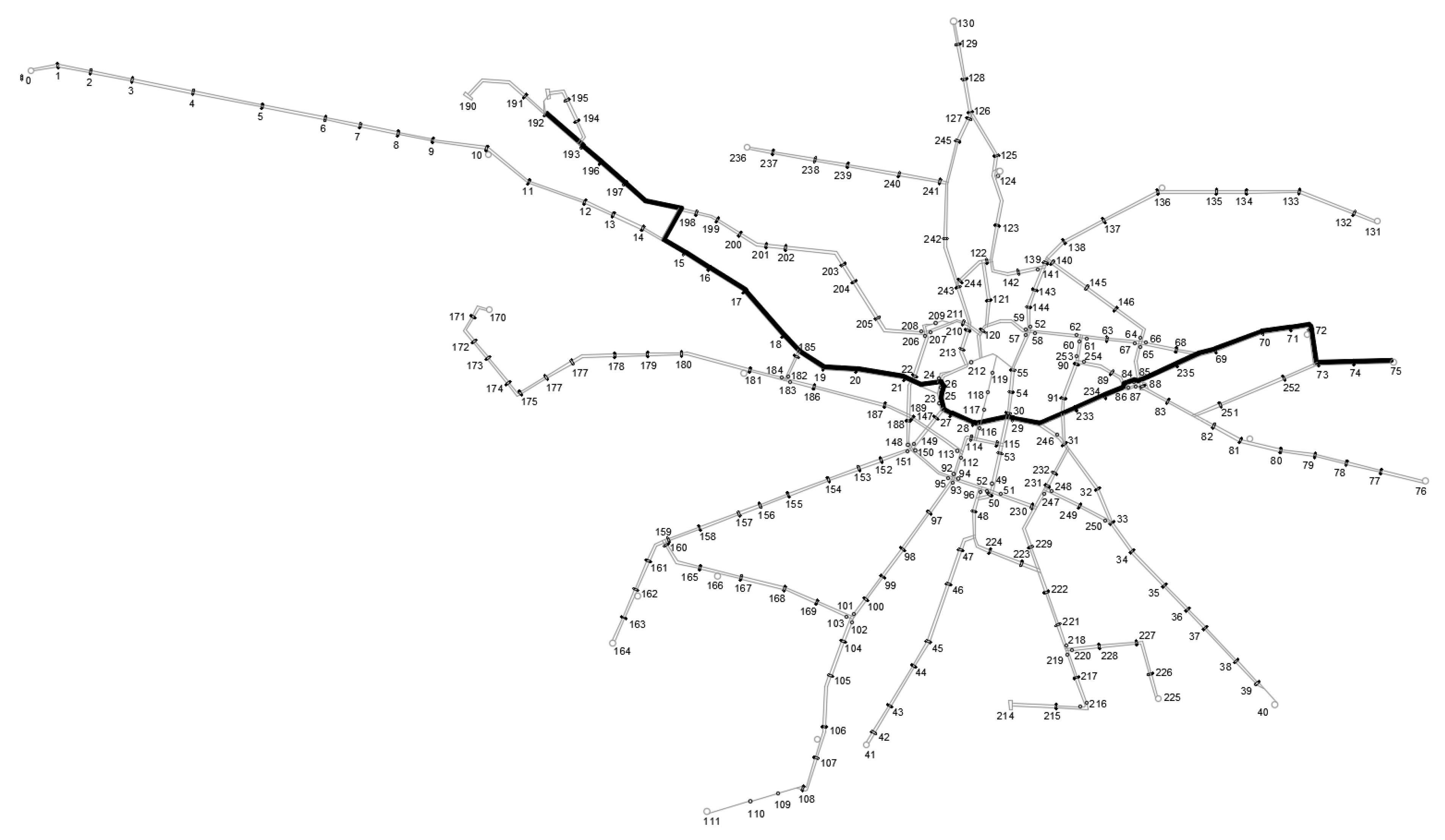
3. Case Study
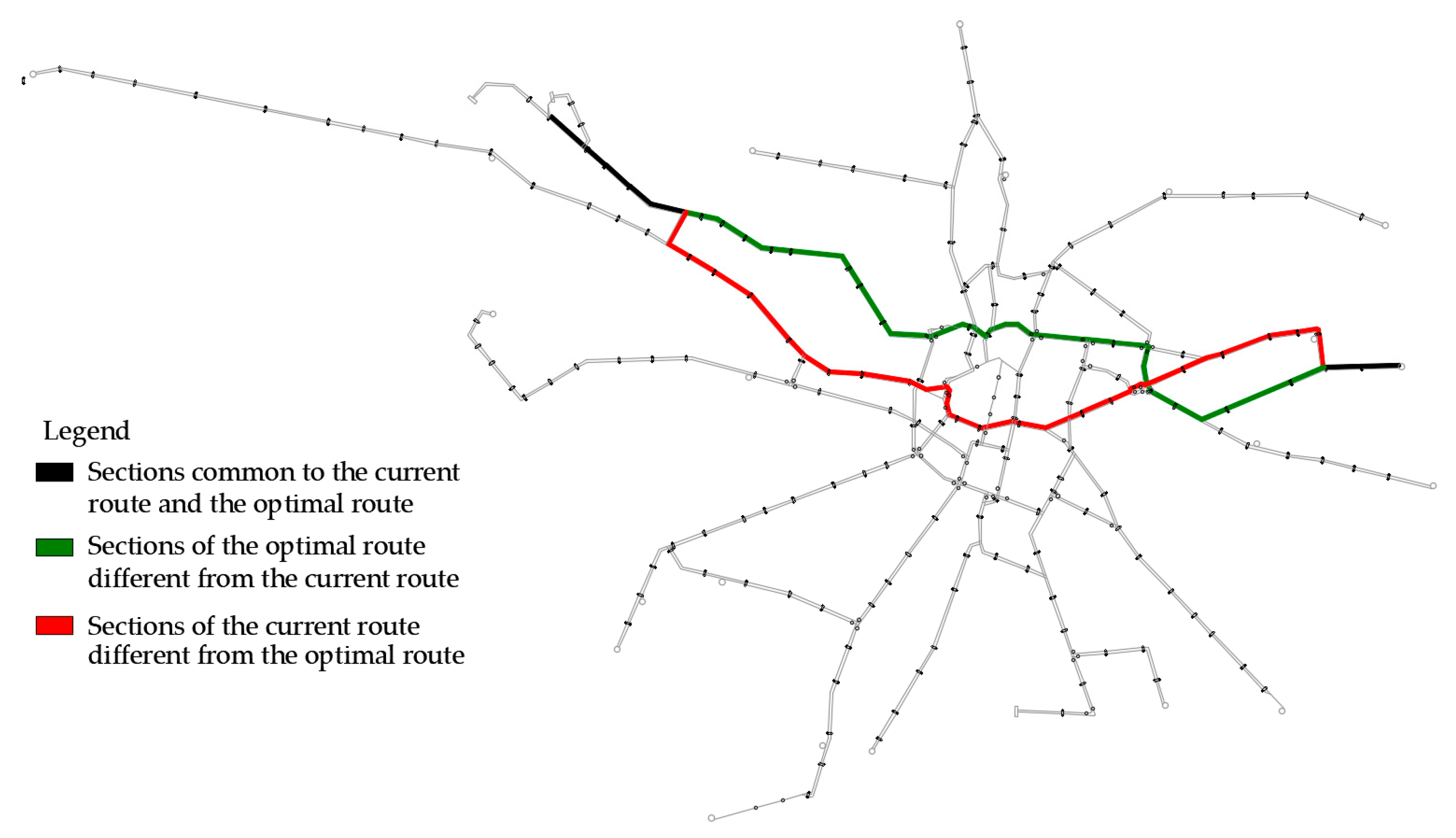
4. Results
5. Discussion
6. Conclusions
Author Contributions
Funding
Institutional Review Board Statement
Informed Consent Statement
Data Availability Statement
Conflicts of Interest
References
- Cascetta, E. Transportation Systems Engineering: Theory and Methods; Springer Science & Business Media: Berlin/Heidelberg, Germany, 2013; Volume 49. [Google Scholar] [CrossRef]
- Zhang, H.; Lu, G.; Lei, Y.; Zhang, G.; Irene, I. A hybrid framework for synchronized passenger and train traffic simulation in an urban rail transit network. Int. J. Rail Transp. 2022, 11, 912–941. [Google Scholar] [CrossRef]
- Alt, B.; Weidmann, U. A stochastic multiple area approach for public transport network design. Public Transp. 2011, 3, 65–87. [Google Scholar] [CrossRef]
- Kowalska, F. Zanieczyszczenie powietrza istotnym zagrożeniem dla zdrowia mieszkańców polskich miast. Refleksje. Pismo Nauk. Stud. I Doktorantów WNPiD UAM 2020, 21, 71–84. [Google Scholar] [CrossRef]
- Siyu, J.; Longjuan, T.; Zhe, L.; Haowei, W.; Ling, H.; Wei, Z.; Qingging, W.; Ruiyun, L.; Zhen, D. The changing health effects of air pollution exposure for respiratory diseases: A multicity study during 2017–2022. Environ. Health 2024, 23, 36. [Google Scholar] [CrossRef]
- Yashendra, S.; Pratik, A.; Vidhi, V.; Siddharth, G. The Impact of Air Pollution on Neurological and Psychiatric Health. Arch. Med. Res. 2024, 55, 103063. [Google Scholar] [CrossRef]
- Orth, H.; Nash, A.; Weidmann, U. Level-Based Approach to Public Transport Network Planning. Transp. Res. Rec. 2015, 2537, 1–12. [Google Scholar] [CrossRef]
- Shao, Z.; Zhang, L.; Han, C.; Meng, L. Measurement and Prediction of Urban Land Traffic Accessibility and Economic Contact Based on GIS: A Case Study of Land Transportation in Shandong Province, China. Int. J. Environ. Res. Public Health 2022, 19, 14867. [Google Scholar] [CrossRef]
- Karoń, G.; Żochowska, R. Problems of Quality of Public Transportation Systems in Smart Cities—Smoothness and Disruptions in Urban Traffic. In Modelling of the Interaction of the Different Vehicles and Various Transport Modes; Springer: Cham, Switzerland, 2020; pp. 383–414. [Google Scholar] [CrossRef]
- Bozzo, R.; Canepa, M.; Carnevali, V.; Genova, R.; Priano, G. Method for analysis and comparison in planning urban surface transport systems. Sustain. City 2012, 155, 931–942. [Google Scholar] [CrossRef]
- Wu, P.; Li, Y.; Li, C. Invulnerability of the Urban Agglomeration Integrated Passenger Transport Network under Emergency Events. Int. J. Environ. Res. Public Health 2023, 20, 450. [Google Scholar] [CrossRef]
- He, X.; Cao, Z.; Zhang, S.; Liang, S.; Zhang, Y.; Ji, T.; Shi, Q. Coordination Investigation of the Economic, Social and Environmental Benefits of Urban Public Transport Infrastructure in 13 Cities, Jiangsu Province, China. Int. J. Environ. Res. Public Health 2020, 17, 6809. [Google Scholar] [CrossRef]
- Kruszyna, M. Investment challenges pertaining to the achievement of the goals of the Mobility Policy based on the analysis of the results of traffic surveys in Wroclaw. Arch. Civ. Eng. 2021, 67, 505–523. [Google Scholar] [CrossRef]
- Kruszyna, M.; Makuch, J. Mobility Nodes as an Extension of the Idea of Transfer Nodes—Solutions for Smaller Rail Stations with an Example from Poland. Sustainability 2023, 15, 2106. [Google Scholar] [CrossRef]
- Owais, M.; Ahmed, A.S.; Moussa, G.S.; Khalil, A.A. Design scheme of multiple-subway lines for minimizing passengers transfers in mega-cities transit networks. Int. J. Rail Transp. 2021, 9, 540–563. [Google Scholar] [CrossRef]
- Owais, M.; Ahmed, A.S.; Moussa, G.S.; Khalil, A.A. Integrating underground line design with existing public transportation systems to increase transit network connectivity: Case study in Greater Cairo. Expert Syst. Appl. 2021, 167, 114183. [Google Scholar] [CrossRef]
- Rutkowska, D.; Piliński, M.; Rutkowski, L. Sieci Neuronowe, Algorytmy Genetyczne i Systemy Rozmyte; Wydawnictwo Naukowe PWN: Warszawa, Poland, 1997. [Google Scholar]
- Carosi, S.; Frangioni, A.; Galli, L.; Girardi, L.; Vallese, G. A matheuristic for integrated timetabling and vehicle scheduling. Transp. Res. Part B 2019, 127, 99–124. [Google Scholar] [CrossRef]
- Schöbel, A. An eigenmodel for iterative line planning, timetabling and vehicle scheduling in public transportation. Transp. Res. Part C 2017, 74, 348–365. [Google Scholar] [CrossRef]
- Ceylan, H.; Ozcan, T. Optimization of headways and departure times in urban bus networks: A case study of Çorlu, Turkey. Adv. Civ. Eng. 2018, 2018, 7094504. [Google Scholar] [CrossRef]
- Pattnaik, S.B.; Mohan, S.; Tom, V.M. Urban Bus Transit Route Network Design Using Genetic Algorithm. J. Transp. Eng. 1998, 124, 368–375. [Google Scholar] [CrossRef]
- Chakroborty, P. Genetic Algorithms for Optimal Urban Transit Network Design. Comput.-Aided Civ. Infrastruct. Eng. 2003, 18, 184–200. [Google Scholar] [CrossRef]
- Owais, M.; Osman, M.K. Complete hierarchical multi-objective genetic algorithm for transit network design problem. Expert Syst. Appl. 2018, 114, 143–154. [Google Scholar] [CrossRef]
- Owais, M.; Osman, M.K.; Moussa, G. Multi-Objective Transit Route Network Design as Set Covering Problem. IEEE Trans. Intell. Transp. Syst. 2016, 17, 670–679. [Google Scholar] [CrossRef]
- Blum, C. Ant colony optimization: Introduction and recent trends. Phys. Life Rev. 2005, 2, 353–373. [Google Scholar] [CrossRef]
- Stützle, T.; Hoos, H. The max-min ant system and local search for combinatorial optimization problems. In Meta-Heuristics: Advances and Trends in Local Search Paradigms for Optimization; Springer: Boston, MA, USA, 1999; pp. 313–329. [Google Scholar] [CrossRef]
- Dorigo, M.; Gambardella, L.M. Ant colonies for the travelling salesman problem. Biosystems 1997, 43, 73–81. [Google Scholar] [CrossRef] [PubMed]
- Yousefikhoshbakht, M.; Didehvar, F.; Rahmati, F.; Ahmed, Z.H. Fixed fleet open vehicle routing problem: Mathematical model and a modified ant colony optimization. Bull. Pol. Acad. Sci. Tech. Sci. 2024, 72, 148253. [Google Scholar] [CrossRef]
- Bell, J.E.; McMullen, P.R. Ant colony optimization techniques for the vehicle routing problem. Adv. Eng. Inform. 2004, 18, 41–48. [Google Scholar] [CrossRef]
- Pang, M.; Wang, X.; Ma, L. Transit route planning for megacities based on demand density of complex networks. Promet-Traffic Transp. 2022, 34, 13–23. [Google Scholar] [CrossRef]
- Yang, Z.; Yu, B. A Parallel Ant Colony Algorithm for Bus Network Optimization. Comput.-Aided Civ. Infrastruct. Eng. 2007, 22, 44–55. [Google Scholar] [CrossRef]
- Katona, G.; Juhász, J.; Lénárt, B. Travel habit based multimodal route planning. Transp. Res. Procedia 2017, 27, 301–308. [Google Scholar] [CrossRef]
- Sahana, S.K.; Jain, A.; Mahanti, P.K. Ant Colony Optimization for Train Scheduling: An Analysis. Int. J. Intell. Syst. Appl. 2014, 2, 29–36. [Google Scholar] [CrossRef]
- Mishra, A.; Kumar, N.; Kharb, S. Priority Based Train Scheduling Method Using ACO in Indian Railway Perspective. IOP Conf. Ser. Mater. Sci. Eng. 2020, 998, 12016. [Google Scholar] [CrossRef]
- Hasany, M.; Shafahi, Y. Ant colony optimisation for finding the optimal railroad path. Transport 2017, 170, 218–230. [Google Scholar] [CrossRef]
- Kumar, A.; Kumar, R.; Aggarwal, A.; Bedi, J. A meta-heuristic-based energy efficient route modelling for EVs integrating start/stop and recapturing energy effect. Sustain. Cities Soc. 2023, 91, 104420. [Google Scholar] [CrossRef]
- Li, Z.; Huang, J. How to Mitigate Traffic Congestion Based on Improved Ant Colony Algorithm: A Case Study of a Congested Old Area of a Metropolis. Sustainability 2019, 11, 1140. [Google Scholar] [CrossRef]
- Bin, Y.; Zhong-Zhen, Y.; Baozhen, Y. An improved ant colony optimization for vehicle routing problem. Eur. J. Oper. Res. 2009, 196, 171–176. [Google Scholar] [CrossRef]
- Yongqiang, L.; Qing, C.; Huagang, X. An Improved Ant Colony Algorithm for the Time-Dependent Vehicle Routing Problem. In Proceedings of the 2010 International Conference on Logistics Engineering and Intelligent Transportation Systems, Wuhan, China, 26–28 November 2010; pp. 1–4. [Google Scholar] [CrossRef]
- Zhang, M.; Ren, H.; Zhou, Y. Research on Global Ship Path Planning Method Based on Improved Ant Colony Algorithm. IEEE Open J. Intell. Transp. Syst. 2023, 4, 143–152. [Google Scholar] [CrossRef]
- Zhang, W.; Gong, X.; Han, G.; Zhao, Y. An Improved Ant Colony Algorithm for Path Planning in One Scenic Area With Many Spots. IEEE Access 2017, 5, 13260–13269. [Google Scholar] [CrossRef]
- Wei, Y.; Jiang, N.; Li, Z.; Zheng, D.; Chen, M.; Zhang, M. An Improved Ant Colony Algorithm for Urban Bus Network Optimization Based on Existing Bus Routes. Int. J. Geo-Inf. 2022, 11, 317. [Google Scholar] [CrossRef]
- Kruszyna, M. NOAH as an Innovative Tool for Modeling the Use of Suburban Railways. Sustainability 2023, 15, 193. [Google Scholar] [CrossRef]
- Korzeń, M.; Kruszyna, M. Modified Ant Colony Optimization as a Means for Evaluating the Variants of the City Railway Underground Section. Int. J. Environ. Res. Public Health 2023, 20, 4960. [Google Scholar] [CrossRef]
- Korzeń, M.; Gisterek, I. Applying Ant Colony Optimization to Reduce Tram Journey Times. Sensors 2024, 24, 6226. [Google Scholar] [CrossRef]

| Current Route | Optimal Route | |
|---|---|---|
| Number of stops | 26 | 26 |
| Effort [-] | 55.9265 | 50.1512 |
| Length [m] | 12,717 | 12,092 |
| Scheduled time [s] | 2400 (40 min) | 2520 (42 min) |
| Real-time (average) [s] | 2684 (44.73 min) | 2505 (41.75 min) |
Disclaimer/Publisher’s Note: The statements, opinions and data contained in all publications are solely those of the individual author(s) and contributor(s) and not of MDPI and/or the editor(s). MDPI and/or the editor(s) disclaim responsibility for any injury to people or property resulting from any ideas, methods, instructions or products referred to in the content. |
© 2025 by the authors. Licensee MDPI, Basel, Switzerland. This article is an open access article distributed under the terms and conditions of the Creative Commons Attribution (CC BY) license (https://creativecommons.org/licenses/by/4.0/).
Share and Cite
Korzeń, M.; Kruszyna, M. Public Transport Planning Using Modified Ant Colony Optimization. Sustainability 2025, 17, 2468. https://doi.org/10.3390/su17062468
Korzeń M, Kruszyna M. Public Transport Planning Using Modified Ant Colony Optimization. Sustainability. 2025; 17(6):2468. https://doi.org/10.3390/su17062468
Chicago/Turabian StyleKorzeń, Mariusz, and Maciej Kruszyna. 2025. "Public Transport Planning Using Modified Ant Colony Optimization" Sustainability 17, no. 6: 2468. https://doi.org/10.3390/su17062468
APA StyleKorzeń, M., & Kruszyna, M. (2025). Public Transport Planning Using Modified Ant Colony Optimization. Sustainability, 17(6), 2468. https://doi.org/10.3390/su17062468