Modeling of Water Inflow Zones in a Swedish Open-Pit Mine with ModelMuse and MODFLOW

Abstract

The Aitik mine is Sweden’s largest open-pit sulfide mine and Europe’s most important producer of gold, silver, and copper. However, the mine faces problems related to water inflow, particularly in the northern zone and western hanging wall sections of the pit, resulting from various mining activities, including blasting, loading, and hauling. The presence of fracture zones within the pit further exacerbates the issue, as continuous mining operations have aggravated the thickness of these fractures, potentially increasing the volume of water inflow. Consequently, this could lead to various geotechnical issues such as slope collapse, and increase the possibility of acid mine drainage formation. This research develops a numerical model using ModelMuse as the graphical user interface and MODFLOW to simulate groundwater flow in the mining pit under different scenarios, by considering the absence, presence, and varying thickness of fracture zones to address the issue. By analyzing these scenarios, the model estimates the volume of water inflow into the pit under steady-state conditions. The results indicate that the presence of a fracture zone plays a crucial role in controlling water inflows by significantly influencing the inflow budget—by 90% for the north shear inflow (NSI) and by 20% for the western hanging wall inflow (WHWI) at deeper depths of the pit. Variations in the fracture zone thickness result in a 15% increase in water inflow at deeper depths of the pit. These findings provide valuable insights for improving mine water management strategies and informing sustainable mine closure planning to mitigate long-term environmental risks.

1. Introduction

One of the main problems in open-pit mining operations is managing the presence of water. With the increasing depth of the mining operation, water flows into the pit through seepage from the upper floor along a specific and complex geological profile. This has a negative impact on mining activity, such as increased pore water pressure resulting in slope failure, the presence of excessive surface water causing longer hauling times, and even sudden water inrush [1]. An uncontrolled water inflow from the ditch also increases the likelihood of acid mine drainage, which adds significant effort to the environmental remediation process during mine closure [2,3,4,5]. However, these problems can be mitigated by generating a robust and sustainable mine water management system through a thorough understanding of the groundwater system in the mining area.

There are several approaches to understanding the characteristics of groundwater flow systems in mining cases, and one of them is through numerical modeling [6,7,8]. These numerical models are often used as predictive tools and cornerstones for designing a robust mine water management system [9,10]. However, one needs to acknowledge the complexity of the hydrogeological setting and consider all possible features that may affect the groundwater flow system through rigorous parameterization [11,12]. Therefore, it is only natural to consider multiple scenarios to represent the most reasonable outcomes and to employ them as critical “thinking tools”.

This study represents the first attempt to simulate steady-state groundwater flow with a focus on the fracture zone in the Aitik mine, as no prior groundwater model exists for this area. The primary objective is to enhance the understanding of how the fracture zone influences groundwater flow behavior in the Aitik mine region, especially, the uncontrolled water inflow into the open pit. ModelMuse [13] was utilized to define the conceptual idea of the model, perform parameterization, and solve the groundwater equation by MODFLOW [14]. The model setup is based on topographical data from the Advanced Spaceborne Thermal Emission and Reflection Radiometer (ASTER) Global Digital Elevation Model (GDEM), high-resolution geological information from fieldwork, and old reports provided by TU Bergakademie Freiberg and Boliden AB from 2015 to 2017. Observation wells collected during an independent measurement campaign in 2017 were used as simulation constraints.

2. Study Area

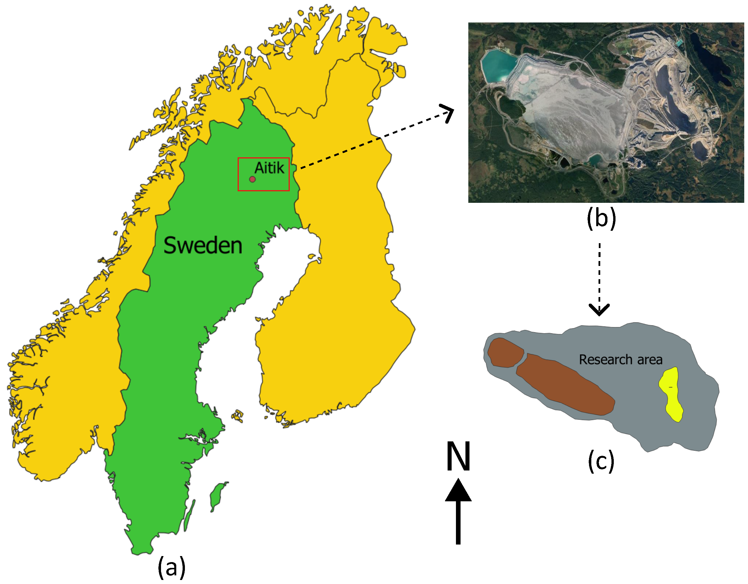
2.1. Geographical Location and Short History

Aitik is the largest open-pit mine in northern Europe, located in Sweden, southeast of Gällivare. Its original Swedish name is Aitikgruvan Gällivare, as shown in Figure 1. The open pit of Aitik is almost 3 km long, 930 m wide, and 450 m deep. The study area lies between a north latitude of 67°1′34.36″ to 67°6′34.88″ and an east latitude of 20°45′49.02″ to 20°59′56.17″.

This area is characterized by a thick glacial moraine profile covering the bedrock, creating a topography of swamps and moraine ridges. Due to these conditions, outcrops are very scarce [15]. It took several decades to discover the valuable mineralization in Aitik from both geophysical and geochemical perspectives. The first boulders containing chalcopyrite were found in 1930 in the Aitik area by Boliden AB, and it was believed that exploitation was not economically viable at that time. This was the case until 1964, when Boliden AB conducted a feasibility study for an open-pit mine to evaluate its economic value. Finally, by 1968, Boliden AB began producing ore at a rate of approximately 2 million tons per year [16].

2.2. Geological Setting

The mineralization in the Aitik area is strongly associated with early orogenic activity. The deposit is situated around 200 km north of the Archaean–Proterozoic paleo boundary in the Fennoscandian Shield, near the volcanic arc environment, as evidenced by the subduction zone of oceanic crust beneath the Archaean craton around 1.9 Ga [17]. These source intrusions led to the formation of the so-called Haparanda suite. Subsequently, the area underwent 160 Ma of modification through strong deformation, including an overprinting mineralizing event of iron oxide–copper–gold (IOCG) [18,19]. The area surrounding Aitik consists of Palaeoproterozoic (ca. 1.9–1.8 Ga) amphibolite facies, intermediate volcanic rocks, and clastic sedimentary rocks, which are intruded by plutonic rocks varying in composition from gabbro to granite [20].

The mining area of Aitik is divided into the footwall ore zone and the hanging wall area, each with distinct structural boundaries and copper grades due to thrusting. The footwall primarily consists of feldspar–biotite–amphibole gneiss and porphyritic quartz monzodiorite, with less than 0.3% Cu containment. Meanwhile, the ore zone comprises garnet-bearing biotite schist and gneiss toward the footwall and muscovite (sericite) toward the hanging wall [21]. The hanging wall itself mainly consists of unmineralized feldspar–biotite–amphibole gneiss, with a thrust contact bounding it from the ore zone. The hanging wall contact of the ore body is sharp and structurally controlled [22].

2.3. Hydrological Setting

The topographical profile of the Aitik mining area before the mining activities (pre-mining) shows that most of the area consisted of bogs with scarce bedrock outcrops. This fact is also confirmed by the presence of residual swamps and small ponds near the mining area, which are surrounded by slightly elevated terrain of pine forest. Although some bedrock outcrops are believed to exist, they are generally covered by a thin layer of alluvial clay or sandy till, depending on the location.

Most of the area is covered by an alluvial profile consisting of a 10–20 m mixture of moraine, fluvioglacial, and peat. However, some areas have additional alluvium coverage due to mining activities. This condition is supported by the fact that waste rock storage facilities (WRSFs) are located in proximity to the mining pit, where mixtures of tailings and potentially acidic formation (PAF) waste rock are stockpiled [23]. Weathered bedrock in contact with the alluvial profile indicates the presence of fracture zones, which result in higher local permeability and, consequently, higher hydraulic conductivity. For instance, the presence of a point of interest regarding the fissure system in the NSI and WHWI zones is noted. The unweathered bedrocks have lower storage and drainable porosity compared to weathered bedrock. Hence, the groundwater capacities vary widely within the region.

The general climatic conditions of the Aitik mining area are characterized by a boreal or subarctic climate with cool summers. The annual precipitation, based on average weather recordings, is approximately 600 mm across the entire Aitik area, with the maximum daily precipitation potentially reaching 30–40 mm during rare heavy rainfall days [23]. A large amount of precipitation is lost in the form of surface runoff; accordingly, groundwater recharge is derived from local sources, totaling around 200 mm/year [24]. During the cold season, bog areas are frozen for 5–6 months, leading to the existence of a low permeability peat layer. Some studies also suggest that the potential existence of permafrost throughout the mining area should be considered [25,26].

Pit dewatering has been actively conducted since 1998 to manage excess water accumulation in the mining pit, with an average pumping rate of approximately 6000 m³/day. However, between 2007 and 2017, the pumping rate increased significantly, reaching a peak of nearly 15,000 m³/day due to an extensive mining expansion campaign during this period. Consequently, the pumping rate is incorporated as a key parameter in our groundwater flow simulations to ensure realistic boundary conditions, as shown in

Table 1. Calculation parameters for the water flow in the Aitik open-pit mine.

Research Area	75 km2
Open-pit length	3 km
Open-pit width	930 m
Open-pit depth	450 m
Average annual precipitation	600 mm [23]
Pit pumping rate	10,000–15,000 m3/day

.

The area surrounding the mine features rivers and distinctive topographical profiles that act as receiving streams, including Leipojoki Creek, the Vassara River, the Lina River, the Ängesån River, and the Kalix River. Additionally, an artificial clarification pond and Sakajärvi Lake are located in the area, along with some small unnamed lakes and ponds on the southern side of the Aitik site.

The inflow zones in the pit area of the Aitik mine are distributed across different levels, predominantly along the hanging wall, and to some extent in the footwall, particularly in the northern section of the pit wall. Field observations suggest there are two major inflow zones between the eastern footwall and the western hanging wall; these two zones are the NSI and WHWI zones, as shown in Figure 2 by point A and point B, respectively. It is believed that both inflow zones are coupled to the fracture zone. In the worst-case scenario, the source of the inflow water supposedly comes from Sakajärvi Lake, as there is no connection between the ditch water near the pit hole and the water flowing out from this fissure system, based on its milieu parameters, as shown in Figure 3.

The WHWI zone is characterized by upper and lower uncontrolled inflows, each with a distinct water source based on its milieu parameters and tracer test results. The upper uncontrolled inflows are most likely related to the ditch water (depicted in Figure 4), while the lower inflows are associated with the seepage water from the TMF, which flows through quaternary pathways above the bedrock, as shown in Figure 5. Hence, both inflows are decoupled from each other.

3. Research Workflow

The typical groundwater modeling workflow [28] is followed in this study and it is depicted in Figure 6.

Initially, a conceptual model representing hydrogeological conditions in the Aitik mine is created based on field reports, geological surveys, and relevant literature. This model identifies key hydrogeological features, such as fracture zones, permeable layers, and groundwater inflow or outflow aspects, which are incorporated as boundary conditions. The groundwater flow simulation is conducted using MODFLOW, with ModelMuse serving as the graphical user interface for model construction, parameterization, and visualization. Afterward, the simulation and observation results are compared, followed by calibration and sensitivity analyses.

3.1. Conceptual Model

The main components of model conceptualization include sources and sinks of water, the distribution of hydraulic properties, and physical boundaries within the research area. The primary goal of this process is to reduce calibration efforts while enhancing both the accuracy and precision of the model.

To the east of the Aitik mining site, the surface water boundary is defined by Sakajärvi Lake, followed by a physical no-flow boundary. This lake is located approximately 1 km from the Aitik site, with an elevation difference of about 35 m. In particular, the physical no-flow boundary extends roughly 2 and 2.5 km from the mining site.

To the west, the clarification pond and the TMF separate the WRSF from the swampy landscape farther west of the Aitik mining site. Topographic maps indicate the presence of some small lakes in this region; however, since they are located far from the area of interest, they are considered negligible, and a physical no-flow boundary is assigned. The clarification pond is located near the TMF, with water from the TMF diverted to a settling pond via a spillway [29]. Around 20% of the water from the clarification pond is discharged into the Lina River [30]. Both the clarification pond and the TMF are defined as notable inner boundary conditions, influencing the water seepage and leakage in specific areas.

To the north, the surface water boundaries include the Lina River, the Vassara River, and the Leipojoki Creek, which are enclosed between Sakajärvi Lake and the clarification pond. These rivers and creeks account for the majority of surface water runoff. Thus, they are subsequently taken up as boundary conditions in the model. The farthest point is located at the Lina River, approximately 2 km from the Aitik mining site. A transitional surface water altitude of 20–25 m exists between the Vassara and Lina rivers, as inferred from the elevation model. Likewise, some parts of Leipojoki Creek are included as a surface water boundary due to its steep gradient, as indicated by its topographic profile.

To the south, there is evidence of small lakes within the swampy area near the southern access road connecting the mining pit facility and the clarification pond facility, which passes by the TMF. This contour is assigned as a specified head boundary condition (BC), consequently supplying water due to its higher altitude. Additionally, there are unnamed small lakes located about 3 km south of the pit in the boggy landscape. Given these boundaries, the modeled area encompasses nearly 75 km².

Due to the complex aquifer setting of the Aitik mine, the conceptual model includes the following four layers: the alluvial layer, transition layer, weathered bedrock, and unweathered bedrock, respectively (see Figure 7). The alluvial layer, predominantly composed of moraine, sandy moraine, and tailings, is situated between the clarification pond and the pit hole. It covers the bedrock by 20 to 40 m. Furthermore, there is a distinct separation in the tailings heap located between the pit hole and the TMF, where environmental waste rock and PAF waste rock are segregated from each other. In addition, the peat profile typically characterizes the alluvial cover in the boggy area on the southern part of the pit hole and has low permeability due to its lithology. The transition layer acts as the interface between alluvial clay and weathered bedrock, consisting of a mixture of more compact moraine and tailings. The weathered bedrock layer is dominated by a bedrock profile, with certain fractured areas representing major inflow zones: NSI and WHWI. Finally, unweathered bedrock forms the deepest layer with very low permeability. General assumptions were made regarding the thickness of the weathered and unweathered bedrock.

In this particular case, three major scenarios are introduced to investigate different possible setups at the specific inflow zones shown in

Table 2. Fracture zone variability on each considered scenario.

Scenario	Fracture Zone	Thickness (m)
1	no	-
2	yes	50
3	yes	100

. The initial thickness of the fracture zone is based on an assumed value to characterize the fissure system within the weathered bedrock. By systematically increasing the thickness of the fracture zone, we simulate the degrees of rock fissure development resulting from the weathering process. This directly influences the hydraulic properties of the bedrock, particularly its permeability and groundwater flow dynamics [31,32].

Governing Equation

This research focuses on solving groundwater simulation based on the steady-state groundwater flow equation derived from Darcy’s Law and the conservation of mass equation [33].

Darcy’s Law is an empirical idea that describes the flow of fluid through a porous medium and its proportional relationship with other influencing factors, such as the cross-sectional area of the medium and the hydraulic head gradient [34]. In this circumstance, Darcy’s Law is applied to simulate the flow of groundwater through complex aquifer systems, such that we have the following:

$$Q=-KA\left({\displaystyle \frac{\Delta h}{\Delta L}}\right)$$

(1)

with Q denoting the volumetric flow rate (or equivalent) to discharge, K denotes the hydraulic conductivity, A denotes the flow area perpendicular to L, and ${\displaystyle \frac{\Delta h}{\Delta L}}$ denotes the hydraulic gradient with respect to hydraulic head (h) and flow path length (L). The hydraulic head is defined as the elevation of the groundwater rise.

To derive the steady-state groundwater flow equation, one must first consider the law of conservation of mass, which states that the rate of fluid entering a volume space is equal to the rate of fluid leaving the volume space, i.e., within saturated porous media, such that we have the following:

$$inflow-outflow=netrateofinflow=0$$

(2)

Consider three components that enter the volume space, namely, $\rho {\upsilon }_x$, $\rho {\upsilon }_y$, and $\rho {\upsilon }_z$, where $\rho$ denotes the density of water and ${\upsilon }_x$, ${\upsilon }_y$, and ${\upsilon }_z$ denote the perceptible velocity of groundwater flow parallel to the x, y, and z axes, respectively. Applying the Taylor series expansion to the rate at which groundwater is flowing out of the volume space and neglecting the higher-order terms, one can compute Equation (2), yielding the following:

$$\begin{array}{cc}\hfill =& \left[\rho {\upsilon }_x+\rho {\upsilon }_y+\rho {\upsilon }_z\right]-\left[\rho {\upsilon }_x+{\displaystyle \frac{\partial }{\partial x}}(\rho {\upsilon }_x)+\rho {\upsilon }_y+{\displaystyle \frac{\partial }{\partial y}}(\rho {\upsilon }_y)+\rho {\upsilon }_z+{\displaystyle \frac{\partial }{\partial z}}(\rho {\upsilon }_z)\right]\hfill \\ \hfill =& -{\displaystyle \frac{\partial }{\partial x}}\left(\rho {\upsilon }_x\right)-{\displaystyle \frac{\partial }{\partial y}}\left(\rho {\upsilon }_y\right)-{\displaystyle \frac{\partial }{\partial z}}\left(\rho {\upsilon }_z\right)=0\hfill \end{array}$$

(3)

If the density of water is assumed to be constant, i.e., the fluid is incompressible, the partial derivative term of density and the density term outside of the derivative can be neglected for the x-direction, such that we have the following:

$$-{\displaystyle \frac{\partial }{\partial x}}\left(\rho {\upsilon }_x\right)=-\left[\rho {\displaystyle \frac{\partial {\upsilon }_x}{\partial x}}+\cancel{{\upsilon }_x{\displaystyle \frac{\partial \rho }{\partial x}}}\right]=\cancel{-\rho {\displaystyle \frac{\partial {\upsilon }_x}{\partial x}}}=-{\displaystyle \frac{\partial {\upsilon }_x}{\partial x}}$$

(4)

The same fashion for y and z directions, such that we have the following:

$$-{\displaystyle \frac{\partial {\upsilon }_x}{\partial x}}-{\displaystyle \frac{\partial {\upsilon }_y}{\partial y}}-{\displaystyle \frac{\partial {\upsilon }_z}{\partial z}}=0$$

(5)

Rearranging Darcy’s Law Equation (1) to ${\displaystyle \frac{Q}{A}}$, which is equivalent to groundwater velocity, and substituting it in Equation (6), yields the steady-state groundwater flow equation:

$$\begin{array}{|c|}\hline {\displaystyle \frac{\partial }{\partial x}}\left(K_x{\displaystyle \frac{\partial h}{\partial x}}\right)+{\displaystyle \frac{\partial }{\partial y}}\left(K_y{\displaystyle \frac{\partial h}{\partial y}}\right)+{\displaystyle \frac{\partial }{\partial z}}\left(K_z{\displaystyle \frac{\partial h}{\partial z}}\right)=0\\ \hline\end{array}$$

(6)

with $K_x$, $K_y$, and $K_z$ denoting the hydraulic conductivities along the x, y, and z axes, respectively.

3.2. Model Design

3.2.1. Elevation Data and Grid System

To obtain elevation information for the Aitik mining site, DEM data from the ASTER GDEM were utilized and downloaded from the NASA database, namely, ASTGTM2_N67E020 and ASTGTM2_N67E021. The most important aspect of defining the grid cell size in numerical modeling is to achieve a reasonably good resolution model without having processing time problems related to computational performance [35,36]. To ensure adequate resolution under these circumstances, the cell size was set to 75 m² with a refined grid cell size of 35 m² at NSI and WHWI areas. A grid smoothing criterion of 1.5 was applied to ensure a smooth transition between high-resolution and lower-resolution cells. The final grid consists of 223 columns and 152 rows. Eventually, the active area was delineated to cover all relevant hydrogeological features within the research area.

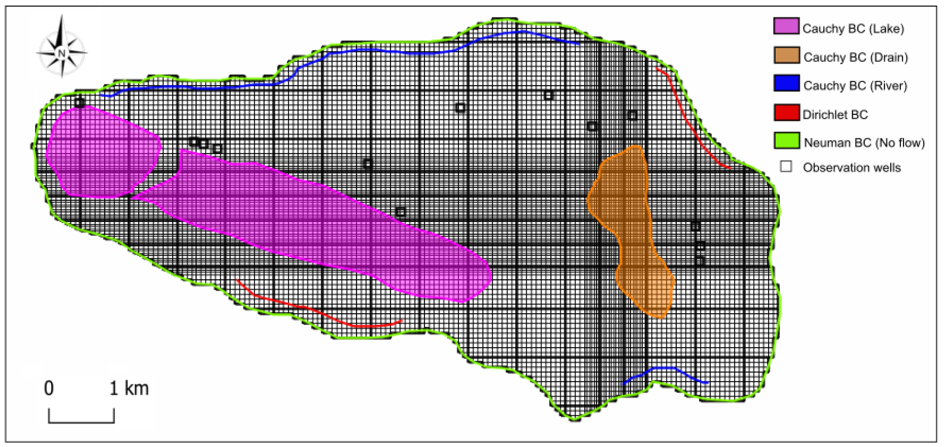
3.2.2. Boundary Conditions

Several boundary conditions were considered to represent the possible hydrological features impacting the research area, as shown in Figure 8. To represent a constant head, a Dirichlet boundary condition (BC) was assigned to Sakajärvi Lake and several unnamed small lakes located in the northeast and southwest of the model domain, with head values fixed between 250 and 270 m and 360 and 380 m, respectively, providing an inexhaustible supply of water or effluent, with unlimited storage capacity, depending on the elevation.

Cauchy BCs were assigned to represent nearby rivers, i.e., the Lina and Vassara Rivers in the northern area, the clarification pond and TMF in the western area, and the pit hole and a small stream in the southeast area of the model domain. For this BC, groundwater can either enter or leave the system as a function of the head. However, this is not the case for the pit hole, as it works solely as a drain. The assigned stages of the river and pond were set based on DEM elevation data, with the bottom elevation varying between 10 and 25 m.

In addition, the Neuman BC was used to distinguish between active and non-active cells, as well as to accommodate precipitation in the research area. An annual precipitation rate of 600 mm was initially set across the model domain [23].

Finally, 13 observation wells were incorporated into the study as simulation constraints. Their locations are also shown in Figure 8.

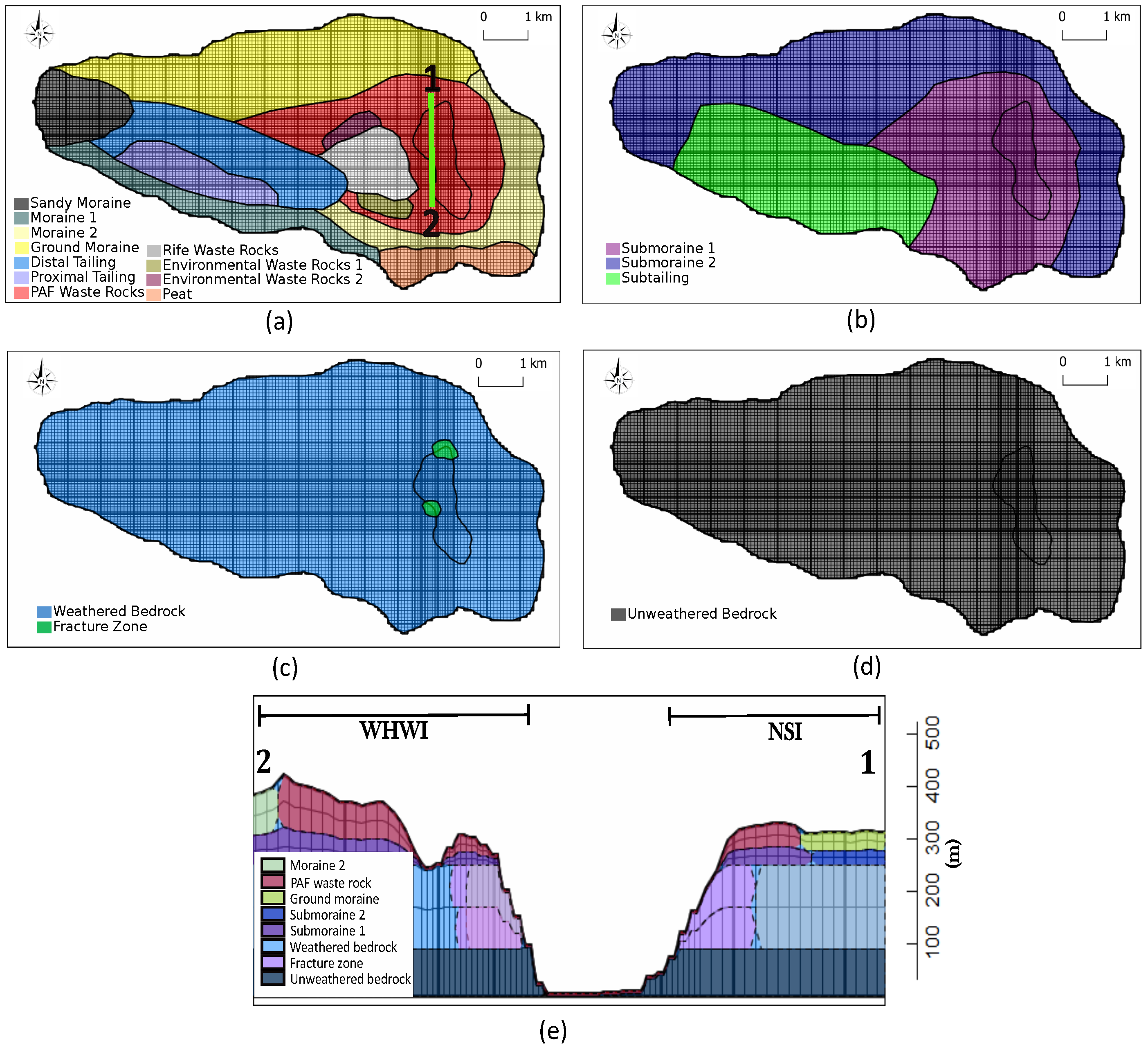
3.2.3. Hydrogeological Unit

Different zones were introduced to represent various hydrogeological units throughout the model domain, along with initial hydraulic conductivity values based on typical values derived from the literature [37], as shown in

Table 3. Hydraulic conductivities of different hydrogeological units assigned in the model before and after calibration.

Hydrogeological Unit	Zone (Parameter Number)	${\mathit{K}}_{\mathit{x}}$ [m/s]
		Before	After
Distal tailings	1	$2.43\times {10}^{-5}$	$2.73\times {10}^{-5}$
Environmental waste rocks 1	2	$1.86\times {10}^{-5}$	$2.54\times {10}^{-5}$
Environmental waste rocks 2	3	$2.08\times {10}^{-5}$	$3.42\times {10}^{-5}$
Ground moraine	4	$5.78\times {10}^{-6}$	$4.19\times {10}^{-6}$
Moraine 1	5	$8.10\times {10}^{-6}$	$8.10\times {10}^{-6}$
Moraine 2	6	$1.04\times {10}^{-5}$	$1.74\times {10}^{-5}$
PAF waste rocks	7	$1.27\times {10}^{-5}$	$9.56\times {10}^{-6}$
Peat	8	$1.16\times {10}^{-6}$	$1.16\times {10}^{-6}$
Proximal tailings	9	$1.85\times {10}^{-5}$	$1.85\times {10}^{-5}$
Rife waste rocks	10	$1.50\times {10}^{-5}$	$2.13\times {10}^{-5}$
Sandy moraine	11	$2.31\times {10}^{-5}$	$2.31\times {10}^{-5}$
Sub-moraine 1	12	$5.79\times {10}^{-7}$	$6.43\times {10}^{-7}$
Sub-moraine 2	13	$6.94\times {10}^{-7}$	$8.83\times {10}^{-7}$
Subtailings	14	$2.31\times {10}^{-7}$	$1.12\times {10}^{-7}$
Weathered bedrock	15	$1.16\times {10}^{-8}$	$7.89\times {10}^{-9}$
Unweathered bedrock	16	$5.79\times {10}^{-9}$	$1.31\times {10}^{-10}$

. Hydraulic conductivity is a measure of a medium’s ability to transmit fluid through its pore spaces and fractures over time. Thus, it varies depending on the permeability and lithological properties of the medium. The assigned hydraulic conductivity was assumed to be anisotropic, such that we have the following:

$$K_x=K_y=10K_z$$

(7)

This means that the vertical hydraulic conductivity ($K_z$) is one-tenth of the lateral hydraulic conductivity, i.e., $K_x$ and $K_y$. The distribution of the hydraulic conductivities is shown in Figure 9. The fracture zone was not assigned an absolute value but rather a relative hydraulic conductivity, which is three orders of magnitude higher than the assigned lateral hydraulic conductivity.

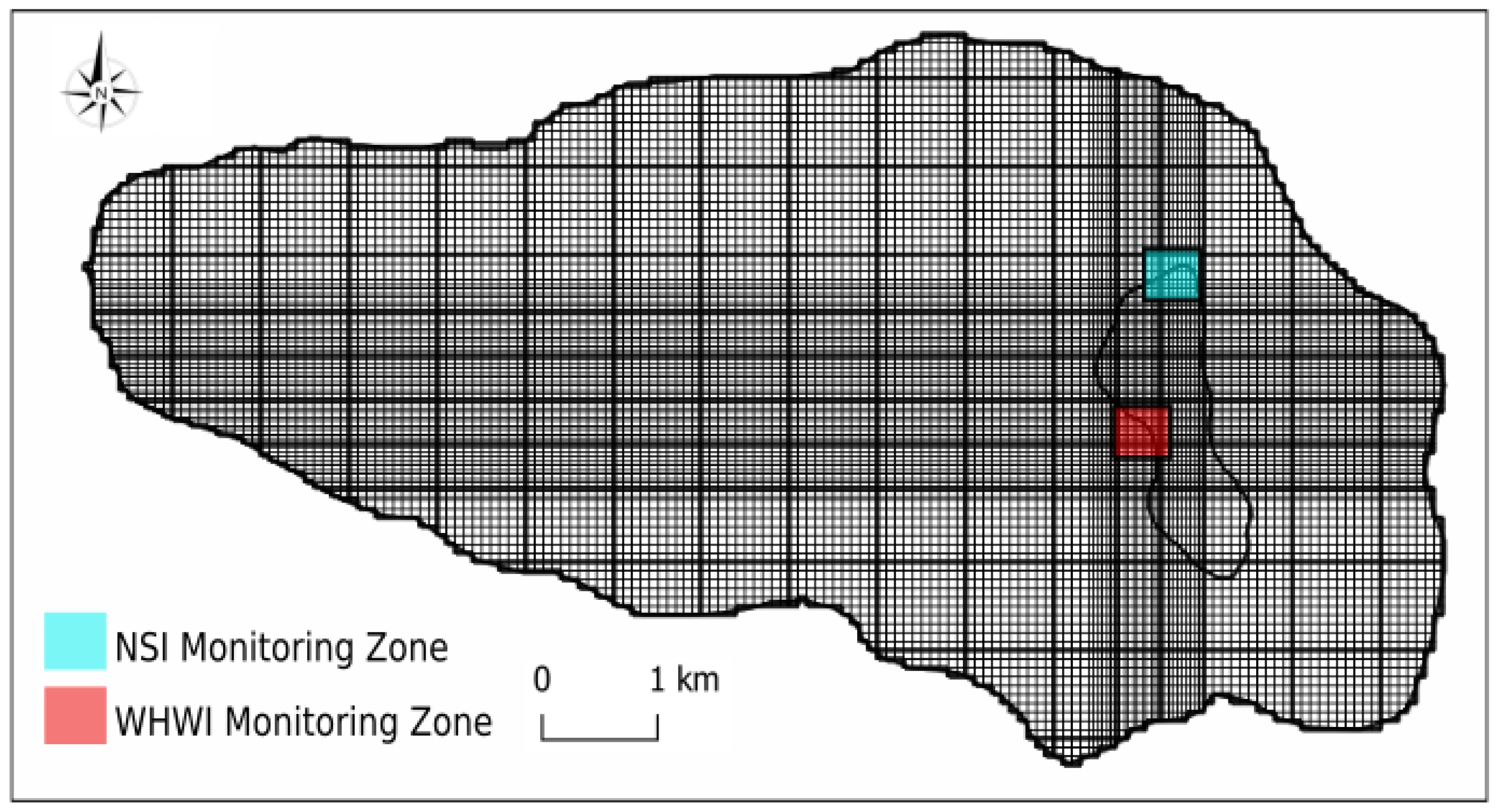
3.2.4. Monitoring Zone

Monitoring zones were adjusted by ZONEBUDGET, a separate post-processing module for MODFLOW, which is used to compute the sub-regional water budget in the model [38]. By using ZONEBUDGET, one can inspect and compare the magnitudes of the lateral and vertical flows between zones for each variation.

In this study, four zones are defined in order to study the flow behaviors on both NSI and WHWI at two different depths, as shown in Figure 10. The upper depth criterion covers the alluvial layer to the transition layer, while the lower criterion covers the weathered bedrock layer to the unweathered bedrock layer.

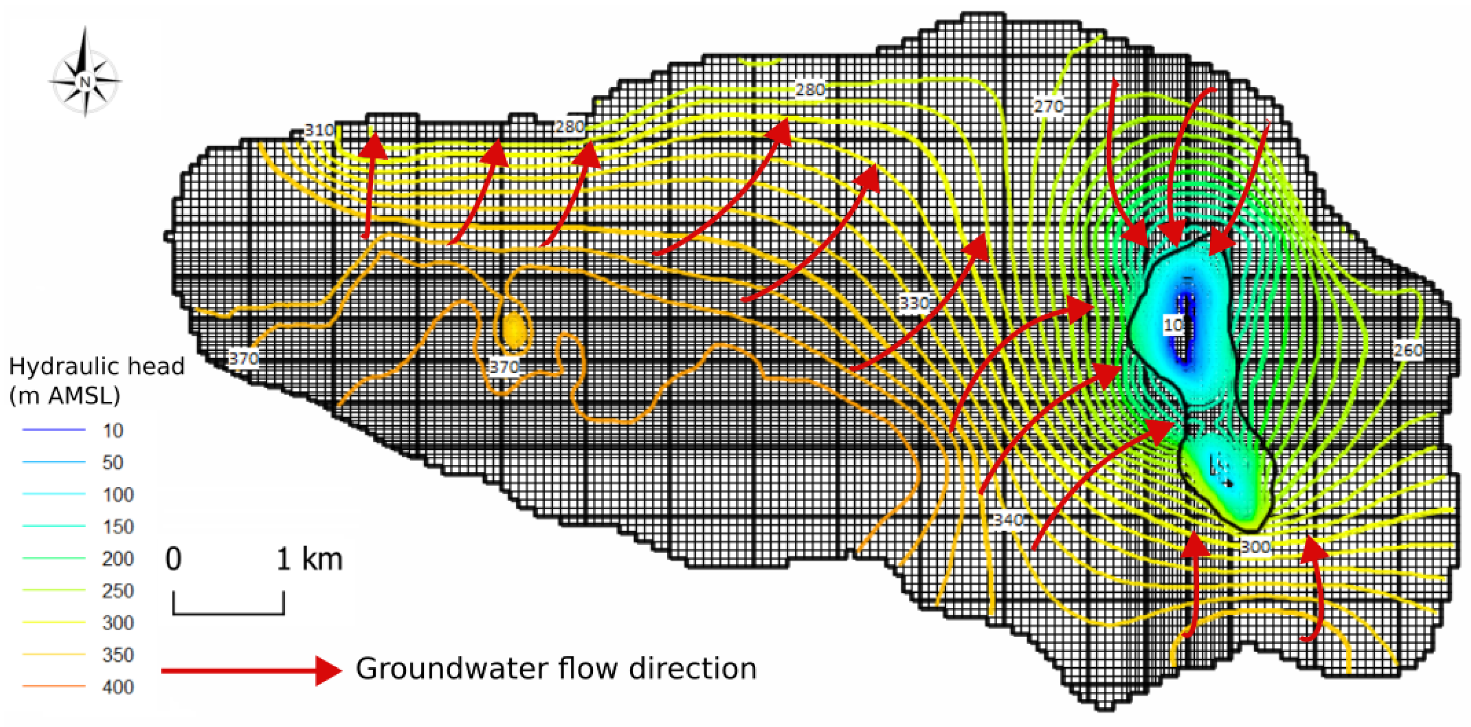
4. Results and Discussion

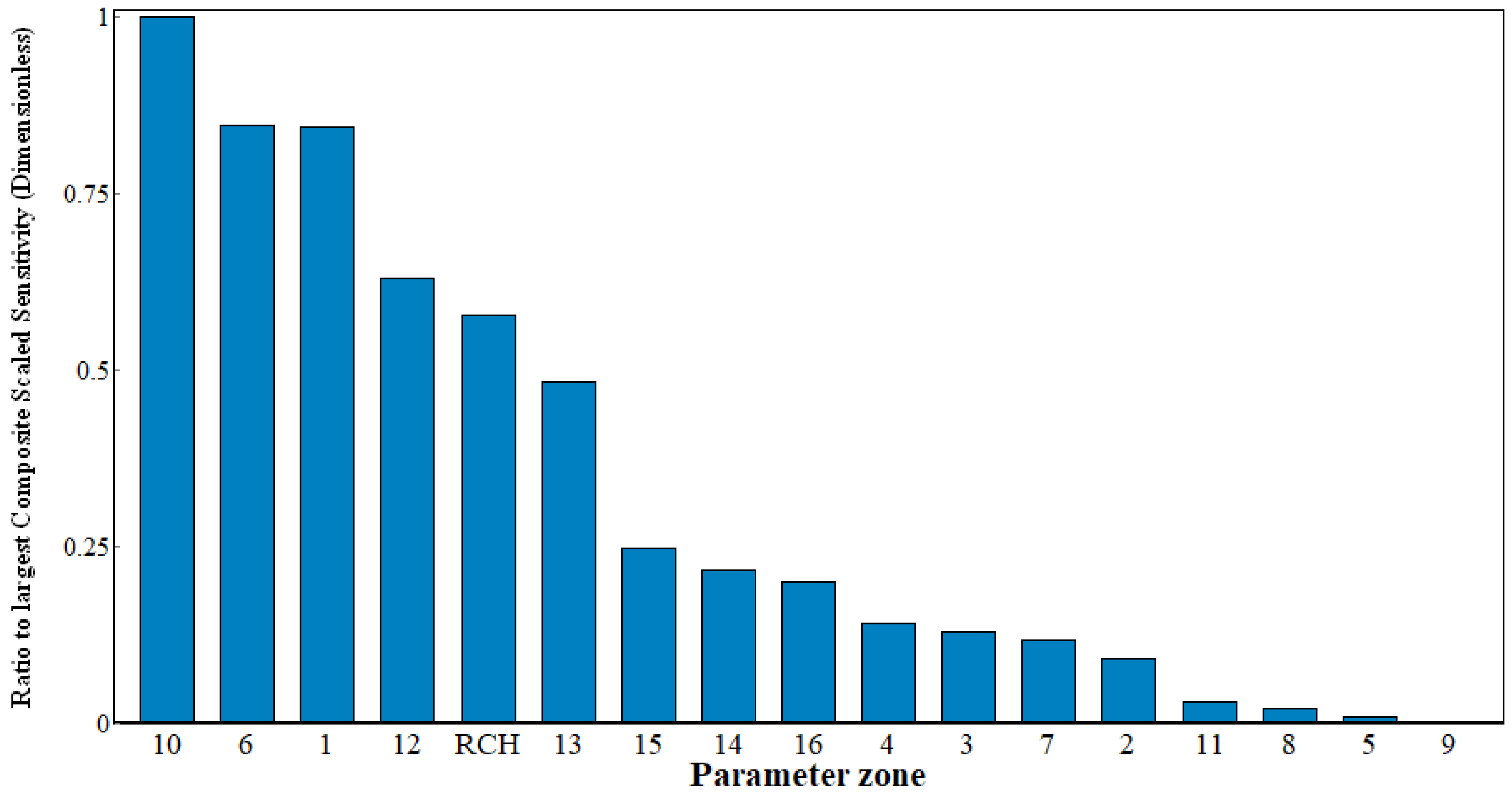
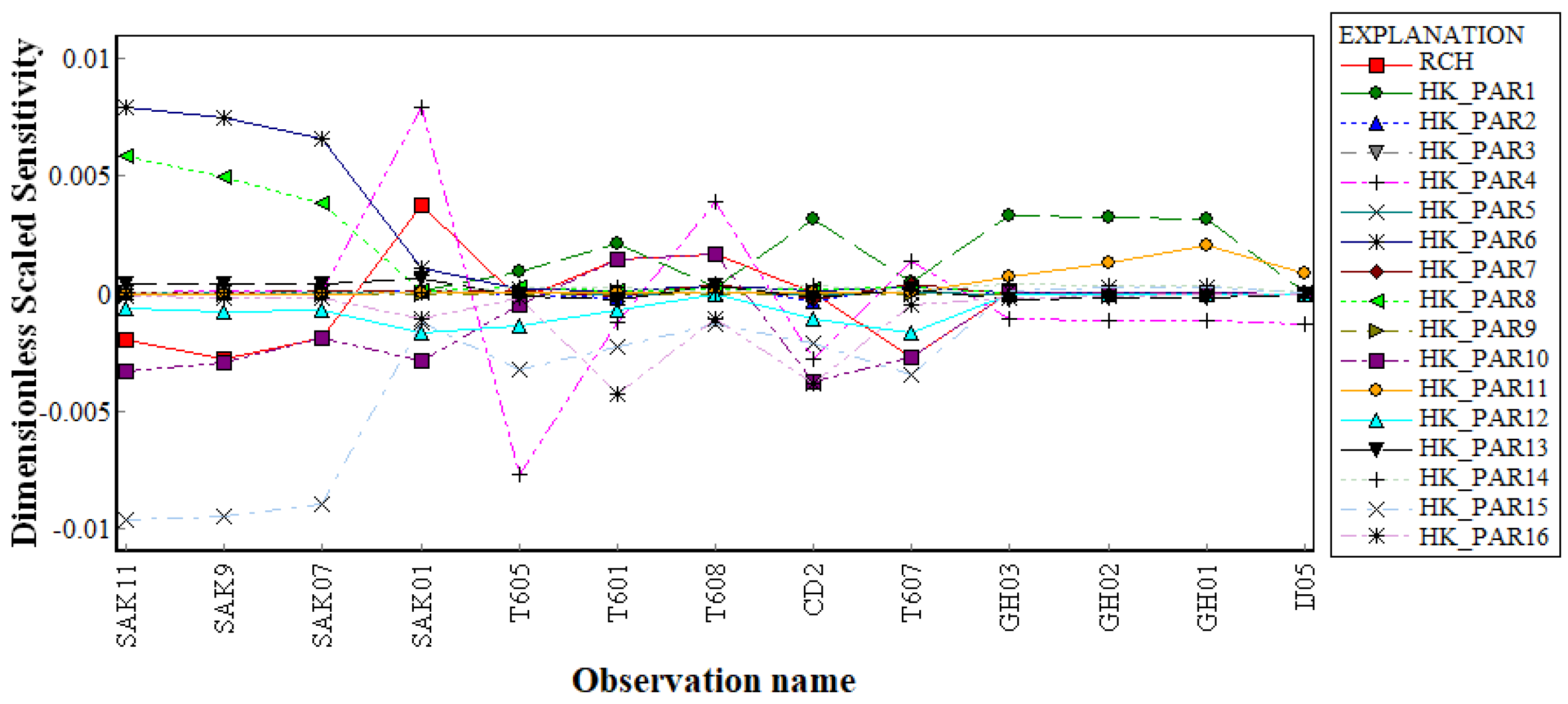
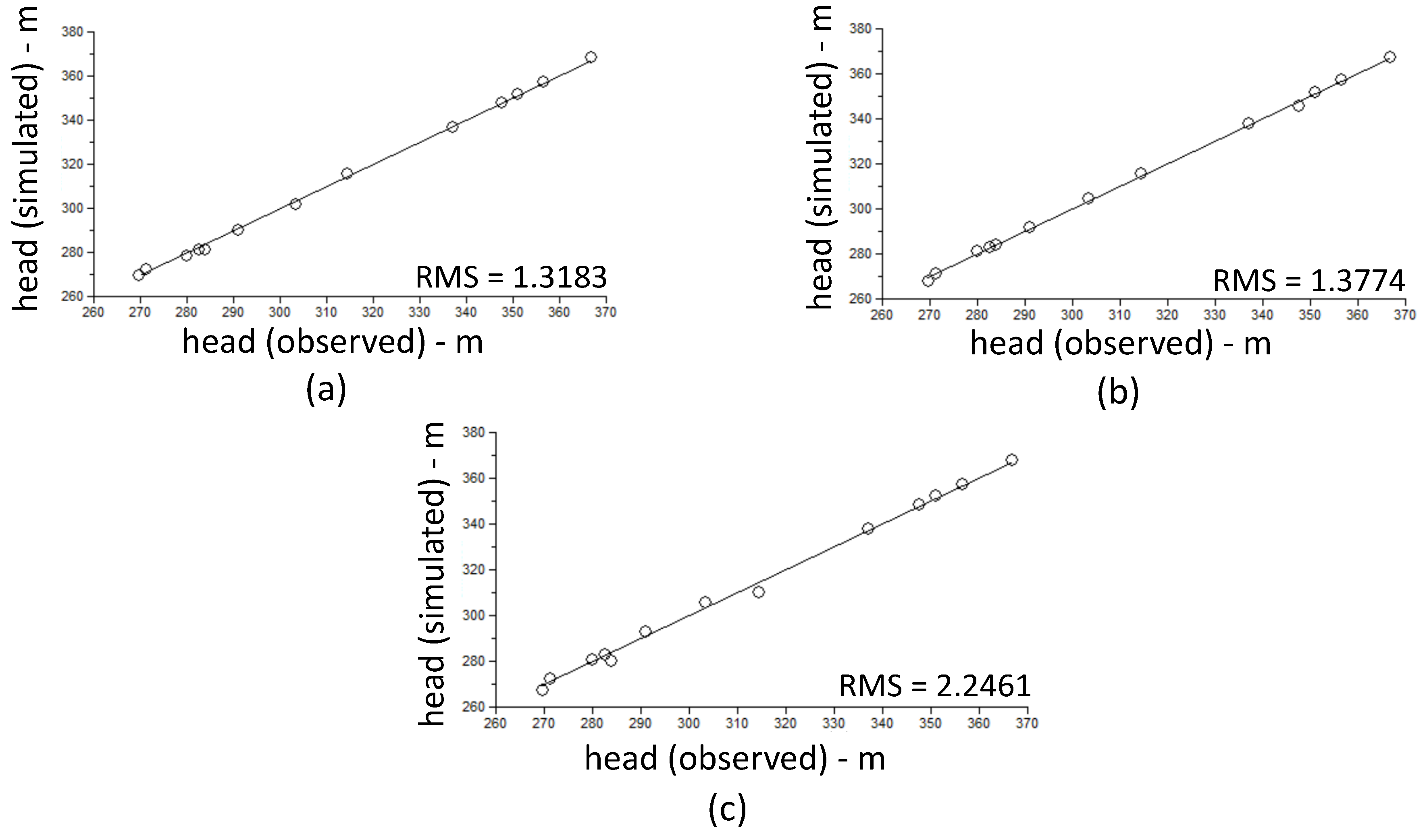
4.1. Calibration and Sensitivity Analysis

The main goal of the calibration step is to compare the level of hydraulic heads on the simulation with the observation, applying hydraulic conductivity as its calibration parameter. The process was done semi-automatically by utilizing UCODE_2014 through ModelMate.

ModelMate is a graphical user interface designed to facilitate the use of model-analysis programs with models [39]. The calibration process involves the following three main steps: forward simulation, sensitivity checking, and parameter estimation.

In the forward simulation, a graph between the simulated head and the observed head was generated to show their correlation. This was measured by an error metric called root mean square (RMS), which calculates the average of the squared differences between observed and simulated heads, such that we have the following:

$$RMS=\sqrt{{\displaystyle \frac{1}{n}}{\displaystyle \sum _{i=1}^n}{\left(ob{s}_i-si{m}_i\right)}^2}$$

(8)

n is the number of observations and $obs$ and $sim$ represent observed and simulated head values, respectively.

Sensitivity checking involves evaluating the significance of parameters with respect to the simulation results. Parameters with small sensitivities, such as those associated with zones 5, 8, 9, 11 (as shown in Figure 11), were set to non-adjustable. On the other hand, Figure 12 shows that the most influential observations in the parameter calculations are SAK11, SAK9, and SAK07. However, since the sum number of observations was insufficient to reliably determine critical values, adequate parameter estimation could not be achieved. Therefore, the parameter estimations were conducted within an 85% confidence interval. Accordingly, the annual precipitation value was reduced to 440 mm to satisfy the calibration requirement. The final adjusted parameters can be seen in Table 3.

The graphs comparing the observed and simulated heads for each scenario using RMS error were produced, with values of 1.3183, 1.3774, and 2.2461, respectively, as shown in Figure 13. A lower value indicates better model performance. Therefore, the first and second scenarios are better than the third scenario in terms of accuracy.

4.2. Evaluation of Different Scenarios

The groundwater balance results for each scenario, as shown in

Table 4. General groundwater balance of the study area in each scenario.

Input in m3day−1		Output in m3day−1
Scenario 1
Constant head	3593	Constant head	5543
River and Lake	13,302	Drains	10,153
Recharge	10,557	River and Lake	11,739
Total	27,452	Total	27,436
Total In - Total Out	16
Discrepancy	0.06
Scenario 2
Constant head	3673	Constant head	5441
River and Lake	13,472	Drains	12,073
Recharge	10,557	River and Lake	10,188
Total	27,702	Total	27,671
Total In - Total Out	31
Discrepancy	0.11
Scenario 3
Constant head	3669	Constant head	5432
River and Lake	13,498	Drains	12,393
Recharge	10,557	River and Lake	9899
Total	27,724	Total	27,689
Total In - Total Out	35
Discrepancy	0.13

, provide an overview of the water budget in the covered area. While these results do not show any notable findings in the overall input and output, there is a slight increase in the output budget on the pit hole (drains) when the fracture zone is employed in the model, inclining by almost 2000 m³/day. Conversely, this increase is offset by a similar decrease in the output through rivers and lakes. However, further examination is necessary to confirm the significance of the fracture zone’s presence.

Another final outcome of the simulation is represented by the groundwater contour lines across the model domain. Since the contour patterns are similar across all three scenarios, only the contour lines of the second scenario are shown here (Figure 14). The equipotential lines represent the hydraulic head contours, with colors in the green–red–blue spectrum indicating decreasing hydraulic head values.

The simulated results indicate a general trend of horizontal groundwater flow moving from the southwest to the northeast within the model domain. Additionally, some groundwater also flows from the southeast, where unnamed small lakes are located.

In the NSI area, the contour lines show a decline toward the pit hole, indicating that groundwater clearly flows northward toward the pit hole, which acts as a sink. In this particular area, tighter equipotential line spacing is observed, which signifies a higher groundwater flow rate. This follows Darcy’s Law, where the flow rate is inversely proportional to the distance between two hydraulic head points and directly proportional to the hydraulic head gradient. The increased groundwater flow rate in the NSI area toward the pit hole is not only due to the lower elevation but also because the hydrogeological unit near the Lina River (ground moraine) has lower hydraulic conductivity compared to the hydrogeological unit surrounding the pit hole.

Similarly, the equipotential lines in the WHWI area also exhibit tighter spacing, indicating a relatively higher groundwater flow rate compared to other areas, such as the Lina River or the clarification pond. This higher flow rate is also influenced by the soil lithology of this region, where waste rock (rife and environmental waste rock) dominates instead of moraine, as the WRSF is located at this specific site.

This also suggests that the runoff catchment from the TMF area toward the pit hole is a highly favorable pathway for groundwater accumulation. Moreover, the presence of the TMF as a river boundary condition enhances groundwater flow due to percolation through the riverbed, resulting in a higher hydraulic head in this area. This could be further verified by analyzing the water budget of the entire model.

However, due to this head-dependent boundary condition, the equipotential lines in the TMF area appear slightly perturbed. This is expected, as the flux across the river boundary depends on the hydraulic head difference between adjacent cells, i.e., water can either leave or enter the boundary depending on the head gradient. If the gradient is negative, water leaves the boundary, and if it is positive, water enters the boundary.

Further investigation was conducted by examining the monitoring zone budgets presented in

Table 5. Groundwater budget of monitoring zones in each scenario.

Scenario	Monitoring Zone	Input in m3day−1		Output in m3day−1
1	Upper NSI	Lateral flow	251	Vertical flow	63
		Recharge	125	Lateral flow	107
				Toward pit hole	206
	Lower NSI	Vertical flow	63	Lateral flow	123
		Lateral flow	613	Toward pit hole	553
	Upper WHWI	Lateral flow	364	Vertical flow	93
		Recharge	151	Lateral flow	74
				Toward pit hole	348
	Lower WHWI	Vertical flow	93	Lateral flow	308
		Lateral flow	423	Toward pit hole	208
2	Upper NSI	Lateral flow	265	Vertical flow	257
		Recharge	125	Lateral flow	28
				Toward pit hole	105
	Lower NSI	Vertical flow	257	Lateral flow	111
		Lateral flow	1231	Toward pit hole	1377
	Upper WHWI	Lateral flow	499	Vertical flow	413
		Recharge	151	Lateral flow	36
				Toward pit hole	201
	Lower WHWI	Vertical flow	413	Lateral flow	503
		Lateral flow	523	Toward pit hole	433
3	Upper NSI	Lateral flow	274	Vertical flow	289
		Recharge	125	Lateral flow	39
				Toward pit hole	71
	Lower NSI	Vertical flow	289	Lateral flow	176
		Lateral flow	1429	Toward pit hole	1542
	Upper WHWI	Lateral flow	512	Vertical flow	496
		Recharge	151	Lateral flow	35
				Toward pit hole	132
	Lower WHWI	Vertical flow	496	Lateral flow	579
		Lateral flow	612	Toward pit hole	529

. By implementing the fracture zone, i.e., between the first and second scenarios, the lateral inflow in the lower monitoring zone increased twofold in the NSI case. The results provide a better representation of the lower uncontrolled inflow, as it predominantly originates from deep lateral percolation rather than vertical percolation. Consequently, a decoupling system between the upper and lower inflow was roughly established. On the other hand, this effect was not observed in the WHWI case, where the lateral inflow at lower depths increased insignificantly, from 423 m³/day to 523 m³/day. Thus, the decoupling system between the upper and lower inflow was not satisfied in the WHWI case.

Although the thickness of the assigned fracture zone was doubled for both cases in the third scenario, the budget did not vary remarkably since it increased the lateral flow of the lower NSI monitoring zone by only 200 m³/day (approximately 15% compared to the second scenario). In the case of WHWI, it increased the lateral flow by 100 m³/day (around 19% compared to the second scenario). Hence, the thickness of the fracture zone is not considered a sensitive parameter in this case.

5. Conclusions

This study examines different aspects of complex groundwater flow processes in an open-pit mining environment through thorough hydrogeological assessments and numerical simulations. It provides insights into the general hydrogeological setting and the major inflow dynamics at the Aitik open-pit mine. The results show that inflow in the NSI case is mainly driven by the presence of fracture zones; however, the WHWI behaves differently, despite both areas exhibiting the same geological properties.

From a mine sustainability and closure planning point of view, this research stresses the importance of understanding groundwater flow behavior at the Aitik mine to assess potential environmental impacts and slope stability issues due to uncontrolled water influx into the pit. For instance, understanding the volume of water inflow into the pit allows for the design of a plausible dewatering system, ensuring the selection of suitable pumps with appropriate pumping capacities to prevent open-pit flooding and avoid possible acid mine drainage formation. Additionally, identifying “hot zones” associated with fracture zones enables the development of an optimized pushback plan and the implementation of mitigation strategies to manage excess water influx if mining operations extend toward these zones.

Further investigation into the WHWI is necessary to understand why its inflow behavior is not similar to that of the NSI. By examining further influencing factors, such as old channel structures or permafrost, one could help refine steady-state simulation and improve the overall understanding of groundwater flow mechanisms. These improvements could serve as the basis for future research focusing on robust transient models and generating more dynamic groundwater flow predictions, ultimately contributing to more accurate and sustainable mine water management practices.

References

1. Wu, Q.; Dong, S.; Li, B.; Zhou, W. Mine water inrush. In Encyclopedia of Sustainability Science and Technology; Springer: New York City, NY, USA, 2018. [Google Scholar]
2. Skousen, J.G.; Ziemkiewicz, P.F.; McDonald, L.M. Acid mine drainage formation, control and treatment: Approaches and strategies. Extr. Ind. Soc. 2019, 6, 241–249. [Google Scholar] [CrossRef]
3. Sakellari, C.; Roumpos, C.; Louloudis, G.; Vasileiou, E. A Review about the Sustainability of Pit Lakes as a Rehabilitation Factor after Mine Closure. Mater. Proc. 2021, 5, 52. [Google Scholar] [CrossRef]
4. Cacciuttolo, C.; Atencio, E. In-Pit Disposal of Mine Tailings for a Sustainable Mine Closure: A Responsible Alternative to Develop Long-Term Green Mining Solutions. Sustainability 2023, 15, 6481. [Google Scholar] [CrossRef]
5. Lemos, M.; Valente, T.; Reis, P.M.; Fonseca, R.; Delbem, I.; Ventura, J.; Magalhães, M. Mineralogical and Geochemical Characterization of Gold Mining Tailings and Their Potential to Generate Acid Mine Drainage (Minas Gerais, Brazil). Minerals 2021, 11, 39. [Google Scholar] [CrossRef]
6. Atkinson, L.; Keeping, P.; Wright, J.; Liu, H. The challenges of dewatering at the Victor Diamond Mine in northern Ontario, Canada. Mine Water Environ. 2010, 29, 99–107. [Google Scholar] [CrossRef]
7. Rapantova, N.; Grmela, A.; Vojtek, D.; Halir, J.; Michalek, B. Ground water flow modelling applications in mining hydrogeology. Mine Water Environ. 2007, 26, 264–270. [Google Scholar] [CrossRef]
8. Surinaidu, L.; Gurunadha Rao, V.; Srinivasa Rao, N.; Srinu, S. Hydrogeological and groundwater modeling studies to estimate the groundwater inflows into the coal Mines at different mine development stages using MODFLOW, Andhra Pradesh, India. Water Resour. Ind. 2014, 7–8, 49–65. [Google Scholar] [CrossRef]
9. Bozic, M.; Nikolic, G.; Milosev, D.; Rudic, Z.; Tomovic, S. Assessment of groundwater management using modflow and benefit–cost analysis. Irrig. Drain. 2014, 63, 550–557. [Google Scholar] [CrossRef]
10. Myers, T. Groundwater management and coal bed methane development in the Powder River Basin of Montana. J. Hydrol. 2009, 368, 178–193. [Google Scholar] [CrossRef]
11. Brown, K.; Trott, S. Groundwater flow models in open pit mining: Can we do better? Mine Water Environ. 2014, 33, 187–190. [Google Scholar] [CrossRef]
12. Leaf, A.T.; Fienen, M.N. Modflow-setup: Robust automation of groundwater model construction. Front. Earth Sci. 2022, 10, 903965. [Google Scholar] [CrossRef]
13. Winston, R.B. ModelMuse: A Graphical User Interface for MODFLOW-2005 and PHAST; US Geological Survey: Reston, VA, USA, 2009.
14. McDonald, M.G.; Harbaugh, A.W. The history of MODFLOW. Ground Water 2003, 41, 280. [Google Scholar] [CrossRef] [PubMed]
15. Malmqvist, D.; Parasnis, D.S. Aitik: Geophysical documentation of a third-generation copper deposit in north Sweden. Geoexploration 1972, 10, 149–200. [Google Scholar] [CrossRef]
16. Zweifel, H. Aitik—geological documentation of a disseminated copper deposit. Sver. Geol. Unders. C 1976, 720, 79. [Google Scholar]
17. Wanhainen, C.; Billström, K.; Martinsson, O.; Stein, H.; Nordin, R. 160 Ma of magmatic/hydrothermal and metamorphic activity in the Gällivare area: Re–Os dating of molybdenite and U–Pb dating of titanite from the Aitik Cu–Au–Ag deposit, northern Sweden. Miner. Depos. 2005, 40, 435–447. [Google Scholar] [CrossRef]
18. Öhlander, B.; Mellqvist, C.; Skiöld, T. Sm–Nd isotope evidence of a collisional event in the Precambrian of northern Sweden. Precambrian Res. 1999, 93, 105–117. [Google Scholar] [CrossRef]
19. Wanhainen, C.; Billström, K.; Martinsson, O. Age, petrology and geochemistry of the porphyritic Aitik intrusion, and its relation to the disseminated Aitik Cu-Au-Ag deposit, northern Sweden. Gff 2006, 128, 273–286. [Google Scholar] [CrossRef]
20. Witschard, F. Bedrock Berggrundskartan 28K Gällivare. 1:50,000. Geol. Surv. Swed. Ai 1996, 98–101. [Google Scholar]
21. Wanhainen, C.; Broman, C.; Martinsson, O.; Magnor, B. Modification of a Palaeoproterozoic porphyry-like system: Integration of structural, geochemical, petrographic, and fluid inclusion data from the Aitik Cu–Au–Ag deposit, northern Sweden. Ore Geol. Rev. 2012, 48, 306–331. [Google Scholar] [CrossRef]
22. Drake, B. Aitik copper mine. Geologi 1992, 2, 19–23. [Google Scholar]
23. Martin, A.; Fraser, C.; Dunbar, D.; Mueller, S.; Eriksson, N. Pit Lake Modelling at the Aitik Mine(Northern Sweden): Importance of Site-Specific Model Inputs and Implications for Closure Planning. Mine Water Circ. Econ. 2017, 1, 154–160. [Google Scholar]
24. Fraile del Río, J. Hydrogeological Model of Aitik Mine Using Leapforg Geo Software. Master’s Thesis, Luleå Tekniska Universitet, Luleå, Sweden, 2015. [Google Scholar]
25. Åkerman, H.J.; Johansson, M. Thawing permafrost and thicker active layers in sub-arctic Sweden. Permafr. Periglac. Process. 2008, 19, 279–292. [Google Scholar] [CrossRef]
26. Johansson, M.; Akerman, H.; Jonasson, C.; Christensen, T.R.; Callaghan, T.V. Increasing permafrost temperatures in subarctic Sweden. In Ninth International Conference on Permafrost; Institute of Northern Engineering, University of Alaska Fairbanks: Fairbanks, Alaska, 2008; Volume 1, pp. 851–856. [Google Scholar]
27. Hoth, N.; Hagedorn, D.; Simon, A. Aitik Water Project-Project Report TU Freiberg. Projectnumber 031002084, 2018. [Google Scholar]
28. Anderson, M.P.; Woessner, W.W.; Hunt, R.J. Applied Groundwater Modeling: Simulation of Flow and Advective Transport; Academic Press: Cambridge, MA, USA, 2015. [Google Scholar]
29. Eriksson, N.; Mueller, S.; Forsgren, A.; Sjöblom, A.; Martin, A.; OKane, M.; Eary, L.; Aronsson, A. Developing closure plans using performance based closure objectives: Aitik Mine (Northern Sweden). Mine Water Circ. Econ. 2017, 2, 822–829. [Google Scholar]
30. Lindvall, M. Strategies for Remediation of Very Large Deposits of Mine Waste: The Aitik mine, Northern Sweden. Ph.D. Thesis, Luleå Tekniska Universitet, Luleå, Sweden, 2005. [Google Scholar]
31. Worthington, S.R.; Davies, G.J.; Alexander, E.C. Enhancement of bedrock permeability by weathering. Earth-Sci. Rev. 2016, 160, 188–202. [Google Scholar] [CrossRef]
32. Hussain, Y.; Campos, J.E.G.; Borges, W.R.; Uagoda, R.E.S.; Hamza, O.; Havenith, H.B. Hydrogeophysical Characterization of Fractured Aquifers for Groundwater Exploration in the Federal District of Brazil. Appl. Sci. 2022, 12, 2509. [Google Scholar] [CrossRef]
33. Istok, J.D. Groundwater Modeling by the Finite Element Method; Wiley Online Library: Hoboken, NJ, USA, 1989; Volume 13. [Google Scholar]
34. Şen, Z. Practical and Applied Hydrogeology; Elsevier: Amsterdam, The Netherlands, 2014. [Google Scholar]
35. Hughes, J.D.; White, J.T. Use of general purpose graphics processing units with MODFLOW. Groundwater 2013, 51, 833–846. [Google Scholar] [CrossRef] [PubMed]
36. Brunner, P.; Simmons, C.T.; Cook, P.G.; Therrien, R. Modeling surface water-groundwater interaction with MODFLOW: Some considerations. Groundwater 2010, 48, 174–180. [Google Scholar] [CrossRef] [PubMed]
37. Domenico, P.A.; Schwartz, F.W. Physical and Chemical Hydrogeology; John Wiley & Sons: Hoboken, NJ, USA, 1997. [Google Scholar]
38. Harbaugh, A.W. A Computer Program for Calculating Subregional Water Budgets Using Results from the US Geological Survey Modular Three-Dimensional Finite-Difference Ground-Water Flow Model; US Geological Survey: Reston, VA, USA, 1990; Volume 90.
39. Banta, E.R. ModelMate—A graphical user interface for model analysis. In US Geological Survey Techniques and Methods; U.S. Geological Survey: Reston, VA, USA, 2011; 31p. [Google Scholar]
Figure 1. (a) Location of the Aitik mine in Sweden; (b) satellite bird view of the Aitik mine; (c) depiction of the active research area along with the clarification pond, the Tailing Mining Facility (TMF), and the open pit.
Sustainability 17 02466 g001
Figure 2. Map of two major inflows related to the NSI (red box A) and WHWI (red box B) with the shear zone represented by the blue line. Red bubbles indicate the water inflow locations, with the size of each bubble corresponding to the inflow intensity. The arrow indicates the north direction. Modified from [24].
Sustainability 17 02466 g002
Figure 3. Field parameters from the northern ditch, clarification pond (red box), surface well samples (yellow box), in-pit well samples (blue box), and the northern shear inflow area (green box) during the sampling campaign in 2017. Modified from [27].
Sustainability 17 02466 g003
Figure 4. Field parameters from the western ditch (red box) and the upper part of the western hanging wall’s inflow area (green box) during the sampling campaign in 2017. Modified from [27].
Sustainability 17 02466 g004
Figure 5. Field parameters from the western ditch (red box) and the lower part of the western hanging wall’s inflow area (green box) during the sampling campaign in 2017. Modified from [27].
Sustainability 17 02466 g005
Figure 6. Groundwater modeling workflow for this study.
Sustainability 17 02466 g006
Figure 7. Stratigraphical conceptualization of the Aitik mining site covering WHWI and NSI from a cross-sectional point of view (the thickness is not drawn to scale).
Sustainability 17 02466 g007
Figure 8. Assigned boundary conditions in the model.
Sustainability 17 02466 g008
Figure 9. (a) Hydrogeological unit zone array assigned to the alluvial layer. (b) Hydrogeological unit zone array assigned to the transition layer. (c) Hydrogeological unit zone array assigned to the weathered bedrock layer. (d) Hydrogeological unit zone array assigned to the unweathered layer. bedrock (e) Cross-sectional view of the hydrogeological unit between points 1 and 2 as shown in (a) from the ModelMuse interface.
Sustainability 17 02466 g009
Figure 10. Assigned monitoring zones.
Sustainability 17 02466 g010
Figure 11. Parameter importance to observations, based on the ratio to the largest composite scaled sensitivity.
Sustainability 17 02466 g011
Figure 12. Observation importance based on the dimensionless scaled sensitivity of the model parameters.
Sustainability 17 02466 g012
Figure 13. Simulated head versus observed head in meters above mean sea level (AMSL) for (a) Scenario 1; (b) Scenario 2; and and (c) Scenario 3, along with their respective RMS errors.
Sustainability 17 02466 g013
Figure 14. Simulated hydraulic head (groundwater) contour lines of the study area. Modified with red arrows to depict groundwater flow direction.
Sustainability 17 02466 g014