Spatial Effects and Driving Factors of Consumption Upgrades on Municipal Solid Waste Eco-Efficiency, Considering Emission Outputs

Abstract

To achieve the goal of building zero-waste cities, managing greenhouse gas (GHG) emissions generated from municipal solid waste (MSW) treatment is a critical step toward carbon neutrality. Waste produced by consumption activities constitutes an essential component of MSW management. Using the Super Slacks-Based Measure Data Envelopment Analysis (SSBM-DEA) model and the Spatial Durbin Model (SDM), this study investigates the spatial impacts of consumption upgrading (CU) on municipal waste management across 30 provinces in China, with a particular focus on GHGs as undesirable outputs. In this study, we construct a framework from the dimensions of consumption level, consumption structure, and green consumption. Additionally, other socioeconomic factors influencing waste management are explored. The results indicate a convergence trend in the uneven distribution of consumption upgrading, with the gaps between regions gradually narrowing. Consumption upgrading significantly enhances the eco-efficiency of local waste management and exhibits notable spatial spillover effects, positively influencing the eco-efficiency of neighboring regions. Furthermore, the promotion effect of consumption upgrading on the central and western regions, compared with the eastern region, is more pronounced. This indicates that the technological catch-up resulting from consumption upgrading, supported by policies, can further enhance the eco-efficiency of MSW. This study also provides insights for other regions transitioning from scale expansion to high-quality development in waste management.

1. Introduction

Municipal solid waste (MSW) management presents a significant challenge in the process of urbanization, as emissions of CO₂, organic pollutants, and hazardous substances pose serious threats to the environment and public health [1]. In 2020, the total amount of solid waste generated globally was estimated at 2.24 billion tons. Given the rapid population growth and the continuous advancement of urbanization, forecasts indicate that, by 2050, annual waste generation will increase significantly by 73% compared with the levels in 2020, with the total amount expected to climb to 3.88 billion tons. In China, MSW generation in 2022 was 311.49 megatons (Mt), an increase of 110% compared with 148.413 Mt in 2006 [2]. Addressing the greenhouse gas (GHG) emissions generated by these entities constitutes a critical domain beyond the energy sector. Currently, waste incineration represents a primary and environmentally benign approach to municipal solid waste disposal [3]. Many countries have implemented MSW management initiatives that effectively manage and reduce waste emissions. The implementation of waste management projects based on green technology has a positive impact in terms of overall emissions reduction, enhancing the capacity handling of existing sites, and predicting a decrease in emission intensity [4]. For instance, the comprehensive urban domestic waste management policy and regulatory framework in Colombia, which was applied in the context of Latin American countries, utilized the Wasteaware benchmark indicators [5]. Certain countries have addressed this issue by improving waste treatment facilities and establishing systems for classified waste collection [6]. This study introduces the concept of MSW eco-efficiency to evaluate the efficiency of MSW management.

Globally, 72% of GHGs are linked to household consumption activities [7]. Consumption upgrading (CU), as a key driver of economic growth, not only alters consumer purchasing behaviors and preferences, but also profoundly impacts the quantity, composition, and spatial distribution of MSW [8]. CU, particularly the increasing preference of residents for environmentally friendly products and services, plays a critical role in promoting the transition of MSW management toward eco-efficiency. The disparity in the quantity and composition of consumption exerts a direct influence on the emissions arising from the treatment of MSW, particularly those emissions associated with organic materials [9], plastics, and so on [10]. However, the impact of CU on the eco-efficiency of MSW presents a complex dynamic [11].

On one hand, as consumers increasingly favor green packaging, recyclable products, and sustainable services, the volume of MSW decreases, and the proportion of recyclable resources in the waste stream increases. Green consumption facilitated by green innovation, such as the utilization of green energy [12] and environmentally friendly products [13], contributes to the reduction of consumption-based carbon emissions. This not only alleviates environmental pressure, but also promotes resource recycling, significantly enhancing eco-efficiency. On the other hand, CU also leads to diversified consumption patterns and accelerated product turnover, introducing new challenges to waste management [14]. These challenges include increased processing complexity, higher costs for waste sorting and collection, and the need for upgrading waste treatment facilities. These emerging trends require MSW management systems to allocate more resources, invest in technological innovation, and enhance infrastructure development. The economic costs encompassing collection, transportation, and disposal account for approximately 61% in Beijing [15]. Furthermore, optimized green vehicle routing [16], enhanced waste collection efficiency, and increased recycling rates will augment the energy and environmental benefits of MSW [17]. In the short-term, such demands may negatively impact eco-efficiency, particularly when resource allocation and treatment capacities fail to keep pace with these evolving requirements.

Consumption structure upgrading refers to the phenomenon where consumers, after meeting their basic living needs, increasingly demand higher-level and more diversified goods and services. In China, the proportion of essential expenditures, such as food and other survival-oriented items, in household consumption has steadily declined, while the share of development, experiential, and service-oriented spending has increased [18]. Empirical studies have shown that the structural upgrading of household consumption promotes the green transformation of household consumption [14].

The enhancement of consumption levels reflects both quantitative growth and a greater focus on quality and service optimization [19]. This elevation drives technological innovation, product upgrades, brand development, and market segmentation, revitalizing the consumer market. The Chinese government strategically emphasizes consumption, highlighting its foundational role in economic development in the “14th Five-Year Plan Proposals”. It also underscores the need to adapt to consumer trends, foster new consumption forms, promote new models and formats, and expand both urban and rural markets. Collaborative efforts by the government, enterprises, and consumers are gradually establishing a market mechanism and cultural environment conducive to green consumption.

The primary objective of this study is to establish the MSW eco-efficiency and to investigate the spatial effects and impacts of consumption upgrading on MSW eco-efficiency across thirty provinces in China. By analyzing the potential interregional influences, the heterogeneous characteristics of eco-efficiency can be explored. Furthermore, the exploration of the effects of influencing factors is expected to yield insights for enhancing MSW eco-efficiency. The subsequent sections of this study are organized as follows: Section 2 reviews literature on MSW eco-efficiency and CU; Section 3 introduces the Super Slacks-Based Measure Data Envelopment Analysis (SSBM-DEA) model with undesirable outputs, the entropy and Technique for Order Preference by Similarity to an Ideal Solution (TOPSIS) model, and the Spatial Durbin Model (SDM); Section 4 delineates the variables and data; Section 5 presents the empirical results; and Section 6 concludes with policy recommendations.

2. Literature Review

2.1. MSW Eco-Efficiency

The concept of “eco-efficiency” was introduced by the World Business Council for Sustainable Development in the early 1990s as a means to promote the transition from unsustainable to sustainable development. “Eco-efficiency” refers to a metric for achieving sustainable development by utilizing resources more effectively, reducing environmental pollution and waste emissions, while simultaneously creating economic value. It emphasizes maximizing economic output with minimal resource consumption and environmental impact. The environmental impacts of MSW primarily encompass gaseous emissions, water discharges, and soil contamination, while open-air landfills also pose threats to human health [20]. Currently, the principal methods for waste disposal encompass landfilling, incineration, composting, and anaerobic digestion (AD). Landfilling is an economically feasible disposal option; however, the methane it generates has a greenhouse effect that is 28 to 36 times more potent than that of carbon dioxide (CO₂), making it the primary gas emitted from landfills [21]. Incineration has emerged as the most direct method for diverting MSW from landfills and is a major waste disposal approach in China [22]. It has also become an alternative strategy for reducing fossil fuel consumption. AD not only recovers energy from the organic fraction of MSW, but also recycles nutrients [23]. Landfill gas collection following incineration for energy recovery and AD represents a primary waste-to-energy (WtE) technology [24]. Composting, on the other hand, is solely applicable to waste with high organic content (such as kitchen waste and garden waste), and it relies on rigorous waste segregation [25].

The measurement of MSW eco-efficiency is jointly determined by resource utilization, environmental impact, and treatment technology, demonstrating a high degree of integration and multidimensionality. Currently, the assessment of MSW eco-efficiency primarily relies on comprehensive indicator systems. The core indicators encompass: environmental impact intensity (GHGs and solid waste generation rate), treatment technology levels (MSW generation and sorting efficiency, classification and collection rate, harmless treatment rate), and the effectiveness of management strategies (policy implementation strength, public participation level, and personal subjective life satisfaction) [26,27,28,29,30,31].

Numerous studies have adopted the classical data envelopment analysis (DEA) approach to investigate the eco-efficiency of economic activities or resource utilization. For instance, some studies have incorporated varying environmental requirements sequentially into DEA to evaluate eco-efficiency by balancing operational and environmental concerns [32]. The DEA model has been widely used to assess both the cost and environmental dimensions of efficiency in the MSW sector [33]. With the advancement of research, scholars have applied various methods to address the limitations of the classical DEA model in measuring eco-efficiency. For example, mixed super-efficiency DEA was employed to measure the eco-efficiency of industrial sectors in China, separating input variables and undesirable output variables into radial and non-radial components to analyze inefficiencies [34]. lo Storto used the generalized directional distance function (GDDF) combined with a DEA model to measure the eco-efficiency of 94 cities in Puglia, Italy, providing MSW services between 2019 and 2021 [31]. In the assessment of eco-efficiency in MSW management, the DEA model and its integration with other models have been extensively utilized. Examples include the generalized directional distance function (GDDF) integrated with DEA [31], stochastic semi-parametric data methodologies [35], and meta-frontier DEA approaches [33]. Among these studies, most treat recycled waste as desirable outputs while integrating unsorted waste into undesirable outputs [36,37]. Alternatively, separately collected waste is considered as desirable outputs, with non-recyclable landfilled waste designated as undesirable outputs [31]. Notably, environmental impacts in the process of MSW management are not accounted for in this framework.

2.2. Consumption Upgrading

The environmental impacts of consumption have been widely studied. Low-carbon green transitions and CU are mutually reinforcing Granger causality factors, with CU significantly promoting low-carbon green transitions [38]. Research has also identified a positive spatial spillover relationship between digital inclusive finance and carbon emissions, where the upgrading of consumption structures enhances the carbon reduction effects of digital finance [39]. Consumer behavior not only exerts a significant influence on the generation and classification of MSW from a micro perspective [40,41], but also, as a crucial engine of the macroeconomy, the complex and dynamic social consumption patterns influence household waste generation, such as food waste [42]. For instance, a study categorizing Chinese provinces based on economic and consumption levels found that different consumption patterns have a significant impact on MSW generation [43]. Moreover, rapid expansion in plastic manufacturing and consumption has created a harmful cycle of pollution and GHG, particularly in households opting for open dumping and burning. However, Petrescu et al. argue that an increase in consumer expenditure generates a decrease in the quantity of municipal waste [40]. The utility theory of consumption emphasizes that, as consumer income levels and preferences evolve, CU manifests as increased demand for higher-quality and more efficient products and services. However, the environmental impacts, especially the influence of CU on MSW eco-efficiency, such as carbon emissions, remain inconclusive [44].

CU, as one of the main manifestations of economic growth, plays a crucial role in the sustained and stable development of the economy and society through the growth of its scale and the adjustment of its structure. The measurement of CU in research mainly includes the upgrading of consumption level and consumption structure [45]. In China, consumer behavior is gradually shifting from survival consumption toward a trend of development and enjoyment consumption. The trend of CU is also manifested in the change of consumption patterns [46]. Furthermore, CU is also measured using an evaluation indicator system that takes into account multiple aspects [47]. With the shift towards more environmentally conscious purchasing behaviors, green consumption occupies a pivotal position in evaluating CU [48]. Unfortunately, no research on CU has taken green consumption into account.

Studies on new economic geography suggest that geographically based sample data tend to exhibit not mutual independence, but rather spatial dependency and spatial agglomeration is closely associated with increasing returns to scale. Within the context of CU, central cities drive local technological transformation and optimize regional innovation, thereby promoting the development of consumption economies in peripheral cities. Both technology inflows and product renewal are more readily absorbed and converted into productivity. Meanwhile, significant regional heterogeneity is observed in the process of CU [46]. Numerous studies have focused on the spatial and temporal variations in eco-efficiency. Zhou and Kong employed an improved three-stage DEA method based on slack measures, treating carbon emissions and three types of industrial waste as undesirable outputs, to evaluate the environmental performance of 30 Chinese provinces from 2004 to 2016 [49]. As CU deepens, MSW is gradually shifting toward technological efficiency and resource sustainability.

In summary, the impact of CU on MSW eco-efficiency remains ambiguous. First, although various methods have been proposed to measure MSW eco-efficiency, most focus on the effects of waste classification while neglecting the impact of carbon emissions within MSW management systems. This study incorporates GHGs as undesirable outputs into the evaluation of MSW eco-efficiency using the SSBM-DEA model. Second, most studies examine MSW eco-efficiency in isolation, failing to account for potential interactions between regions. By employing the SDM model, this paper captures spatial spillover effects, providing additional insights and drawing several valuable conclusions. Third, while previous literature often uses consumption structure upgrading or consumption level upgrading as isolated indicators of CU, this study integrates green consumption into the evaluation, establishing a comprehensive system for assessing CU.

2.3. Hypotheses

The core–periphery theory elucidates the imbalance and dynamism of interregional economic development, emphasizing the interdependence and interaction between core and peripheral regions. With the continuous advancement of consumption upgrading, the proliferation of the green living concept, and innovations in environmental protection technologies, the demand for refined and efficient waste management within and between cities has been escalating [43]. The transformation of consumption patterns has fostered an enhanced awareness of commodity recycling and resource conservation. During this process, the accelerated circulation of substantial waste reduction flows, resource recovery flows, and technological innovation flows has not only spearheaded new trends in ecological waste treatment in large cities, but also driven technological upgrades and model innovations in waste management among surrounding small and medium-sized cities. Research on new economic geography suggests a close correlation between spatial agglomeration and increasing returns to scale [50]. In terms of CU, central cities drive local technological transformation and optimization of regional innovation, stimulating the development of the consumer economy in peripheral cities. Both inflowing technologies and upgraded products are readily absorbed and converted into productivity. This promotes the transition of urban solid waste management towards technological conservation and resource sustainability. The core–periphery structure fosters technological complementarity among multiple central and peripheral cities, breaking geographical distance barriers and enhancing the MSW eco-efficiency [51].

The spillover effect of CU on the MSW eco-efficiency can manifest as either positive or negative externalities. On one hand, when the level of MSW management in a particular region is enhanced, exemplified by the adoption of advanced treatment technologies and the implementation of stringent sorting and recycling systems, it may catalyze improvements in waste management practices in neighboring areas, thereby mitigating environmental pollution and fostering a positive demonstrative effect. Conversely, CU, through its influence on industrial scale and structural effects, may propagate negative environmental externalities across cities via inter-city industrial linkages, leading to increased resource consumption and pollutant emissions [38]. If MSW management in a region is inadequate, characterized by illegal dumping, improper disposal, and so forth, this may result in the dissemination of pollutants to surrounding areas, exacerbating environmental pollution and giving rise to a negative spatial spillover effect [52].

Based on empirical analysis, conceptual development, and model formulation, this study posits the following hypotheses concerning the impact of CU on MSW eco-efficiency.

H1. 

CU exhibits significant regional variations. These variations can influence MSW eco-efficiency differently, with some regions benefitting more from consumption patterns that promote waste reduction and recycling than others.

H2. 

MSW eco-efficiency demonstrates robust spatial autocorrelation features. The influence of consumption upgrading on MSW eco-efficiency manifests strong spatial spillover effects, suggesting that improvements in one area can positively or negatively affect neighboring regions.

H3. 

The influence of consumption upgrading on MSW eco-efficiency exhibits significant spatial heterogeneity.

3. Methodology

3.1. Calculation of GHGs from MSW Treatment

In China, various waste management and treatment approaches encompass landfills, incineration processes, and composting techniques. Referring to previous studies [53,54,55], to quantify GHG emissions resulting from MSW disposal in the country, we employed the bottom-up inventory methodology as advocated by the Intergovernmental Panel on Climate Change [56]. Furthermore,

Table A1. Composition of domestic waste in different areas of China.

Region	Food Waste	Paper	Plastic	Textiles	Wood	Rubber and Leather	Metal	Glass	Others
Northern China	50.76	11.57	11.77	4.18	4.29	1.6	2.75	3.92	0.92
Northeast China	58.87	7.24	11.14	2.69	5.94	5.5	1.08	3	6.31
Eastern China	64.5	8.65	12.45	2.3	1.77	0.8	0.65	2.92	2.02
Central China	49.42	3.12	8.61	4.04	4.75	1.5	0.76	0.81	8.3
Southern China	51.18	11.81	13.49	3.71	2.03	0.9	0.74	1.86	5.85
Southwest China	52.22	9.98	12.61	2.81	2.5	4.1	1.16	1.62	7.11
Northwest China	51.93	6.85	9.41	2.72	1.75	1.6	1.21	2.89	4.25
Data Sources	(Bian [12]; Cai [57]; Gu [13]; Lou [56])

in Appendix A provides a detailed breakdown of the components of MSW across diverse regions of China.

3.1.1. GHG Emissions from Landfills

A sanitary landfill constitutes a fundamental approach to waste disposal. The default methodology recommended by the Intergovernmental Panel on Climate Change (IPCC) was utilized to CH₄ emissions eman landfills:

$$E_{landf-C{H}_4}={\sum }_i{MSW}_{lf}\times {MSW}_i\times MCF\times {DOC}_i\times {DOC}_f\times F\times {\displaystyle \frac{16}{12}}\times \left(1-R\right)\times \left(1-O\right)$$

(1)

where $E_{landf-C{H}_4}$ signifies the ${CH}_4$ emissions emanating from landfills, totaling 10,000 tons. ${MSW}_{lf}$ represents the total quantity of MSW landfilled. ${MSW}_{lf}$ denotes the proportion of waste comprising the $i$-th component. $MCF$ stands for the ${CH}_4$ correction factor, which varies based on the type of landfill management. ${DOC}_i$ refers to the degradable organic carbon content of the $i$-th component, expressed in kilograms of carbon per kilogram of waste. ${DOC}_f$ signifies the fraction of DOC that is decomposable. F represents the proportion of ${CH}_4$ in the landfill gas. The term 16/12 accounts for the molecular weight ratio of ${CH}_4$ to carbon. $R$ denotes the amount of ${CH}_4$ that is recovered. Finally, O represents the oxidation factor.

Due to variations in landfill size and management practices, the input values for MCF, OX, and R deviate from the default values recommended by the IPCC, incorporating expert judgment as well. Specifically, the values for ${DOC}_i$ values were from the previous study [57]. ${DOC}_f$ is 0.5, $MCF$ is 0.96, and F is 0.5. R is 0.24 and O is 0.1, as per reference [58].

3.1.2. GHG Emissions from Incineration

Incineration boasts a robust processing capacity and does not restrict the type of waste that can be processed. The primary GHGs emitted during incineration are CO₂ and N₂O. The calculation formulas for these emissions are outlined as follows [56]:

$$E_{inc-{CO}_2}={\sum }_i{MSW}_{inc}\times {MSW}_i\times {dm}_i\times {CF}_i\times {FCF}_i\times {OF}_i\times {\displaystyle \frac{44}{12}}$$

(2)

$$E_{inc-N_{2}O}={\sum }_i{MSW}_{inc}\times {EF}_1$$

(3)

where $E_{inc-{CO}_2}$ and $E_{inc-N_{2}O}$ denote the emissions of ${CO}_2$ and $N_{2}O$, respectively. ${MSW}_{inc}$ represents the total quantity of municipal solid waste processed through incineration. The variable ${dm}_i$ stands for the dry matter content of the i-th component in the incineration process. ${dm}_i$ signifies the proportion of carbon within the dry matter of the i-th component. ${FCF}_i$ represents the fraction of mineral carbon in the total carbon content of the i-th component. ${OF}_i$ is the oxidation factor, assigned a value of 1. ${EF}_1$ is the emission factor for $N_{2}O$, set at 50 g of $N_{2}O$ per ton of waste processed. The values of other emission factors are detailed in

Table A2. Emission factors for different waste components during incineration.

Emission Factors	Paper	Wood	Textiles	Food Waste	Plastic	Rubber and Leather	Others
dmi	0.9	0.85	0.8	0.4	1	0.84	0.9
CFi	0.46	0.5	0.5	0.38	0.75	0.67	0.03
FCFi	0.01	0.01	0.2	0.01	1	0.2	1
Data Sources	[56]

located in Appendix A.

3.1.3. GHG Emissions from Composts

Composting entails the process of waste treatment through two fermentation stages: primary and secondary, both of which utilize aerobic conditions. During this process, the primary GHGs emitted are ${CH}_4$ and $N_{2}O$.

$$E_{comp-{CH}_4}={\sum }_i{MSW}_{comp}\times {EF}_2$$

(4)

$$E_{comp-N_{2}O}={\sum }_i{MSW}_{comp}\times {EF}_3$$

(5)

where $E_{comp-{CH}_4}$ and ${\mathrm{E}}_{comp-N_{2}O}$ are, respectively, the ${CH}_4$ and $N_{2}O$ emissions of MSW compost; ${MSW}_{comp}$ is the amount of processed MSW compost; ${EF}_2$ is the ${CH}_4$ emission factor for the composting process, with a default value of 4 g/kg MSW; and ${EF}_3$ is the $N_{2}O$ emission factor for the composting process, with a default value of 0.3 g/kg MSW.

3.2. SSBM-DEA Efficiency Model with Undesirable Output

DEA is a commonly utilized nonparametric approach for assessing technical efficiency, particularly in the context of eco-efficiency evaluations. The traditional DEA method employs a radial and angular measurement technique, which enhances the performance of inefficient decision-making units (DMUs) by proportionally adjusting all input or output factors either up or down. The SBM-DEA model does not presume radial improvements in inputs or outputs; instead, it permits non-proportional changes by simultaneously adjusting multiple input and output indicators. Furthermore, the weights are automatically optimized by the model, thereby providing greater flexibility in reflecting the multidimensional optimization requirements in actual production processes [59]. The SSBM-DEA model, however, is a methodological framework that essentially integrates the concept of super-efficiency with the SBM model. Its core principle lies in the removal of existing efficient evaluation units from the set and the subsequent re-evaluation based on this adjustment [60]. Therefore, it permits the efficiency score of effective DMUs to surpass the threshold of 1, thereby providing a more accurate measurement for DMUs with an SBM score above 1 [20]. This SSBM-DEA efficiency model is specifically designed to effectively differentiate between multiple efficient decision units.

The SSBM model measures all relaxation variables and includes all sources of inefficiency [61]. Under the assumption of variable return to scale, the SSBM-DEA model with unexpected outputs evaluates the eco-efficiency of the MSW system. The settings of the model are as follows [62]:

$${\rho }^{\mathrm{*}}=min{\displaystyle \frac{1+\frac{1}{m}{\sum }_{i=1}^m\frac{s_i^{-}}{x_{io}}}{1-\frac{1}{s_1+s_2}\left({\sum }_{r=1}^{s_1}\frac{s_r^{+}}{y_{io}^g}+{\sum }_{t=1}^{s_2}\frac{s_t^{b-}}{y_{to}^b}\right)}}$$

$$s.t.\left\{\begin{array}{c}{\sum }_{j=1,j\ne 0}^n{x}_{ij}{\lambda }_j-s_i^{-}\le x_{io}\\ {\sum }_{j=1,j\ne 0}^n{y}_{rj}{\lambda }_j-s_r^{+}\ge x_{io}\\ {\sum }_{j=1,j\ne 0}^n{y}_{tj}{\lambda }_j-s_t^{b-}\le x_{io}\\ 1-{\displaystyle \frac{1}{s_1+s_2}}\left({\sum }_{r=1}^{s_1}{\displaystyle \frac{s_r^{+}}{y_{io}^g}}+{\sum }_{t=1}^{s_2}{\displaystyle \frac{s_t^{b-}}{y_{to}^b}}\right)>0\\ s^{-},s^{+},\lambda \ge 0;\end{array}\right.$$

(6)

where i = 1, 2, …, m; r = 1, 2, …, s; and j = 1, 2, …, n (j ≠ o). There are n DMU_j (j = 1, 2, …, n); There are m inputs for each DMU, x_i = (i = 1, 2, …, s_m), the desirable output is y^g (r = 1, 2, …, s₁), and the undesirable output is y^b (r = 1, 2, …, s₂). ${\mathrm{s}}_{\mathrm{i}}^{-}$, ${\mathrm{s}}_{\mathrm{r}}^{+}$, and ${\mathrm{s}}_{\mathrm{t}}^{\mathrm{b}-}$ are the slack variables of input, desirable output, and undesirable output. $\mathsf{\lambda }$ is the weight; ${\rho }^{\mathrm{*}}$ is the eco-efficiency of DMU: the higher the efficiency value, the higher the level of sustainable development. An efficiency value greater than 1 indicates that the eco-efficiency of the year is in the optimal state.

3.3. Measurement of CU

The Entropy-TOPSIS model is a multi-attribute decision analysis method used to evaluate and select optimal decision schemes. This model combines the entropy method with the TOPSIS approach to address multi-attribute decision problems characterized by ambiguity and uncertainty. The entropy method, as an objective weighting approach, effectively eliminates the influence of subjective judgment on evaluation results. The smaller the information entropy of an indicator, the greater the variation in its values, indicating that the indicator provides more information and plays a more significant role in the comprehensive evaluation. Consequently, its weight in the model increases accordingly. With reference to Jiang (2022), this paper establishes the following indicator system for consumption upgrading using the entropy weight method [63].

First, calculate the proportion of indicator values: $P_{ij}=x_{ij}^{\prime }/\sum _{i=1}^n{x}_{ij}^{\prime }$. Then calculate the information entropy value: $E_j=-{\displaystyle \raisebox{1ex}{$1$}\!\left/ \!\raisebox{-1ex}{$ln n$}\right.}\sum _{i=1}^n(P_{ij}\ast ln{P}_{ij})$. Finally, determine the weights of each indicator: $W_j=(1-E_j)/{\sum }_{j=1}^m(1-E_j$).

Based on the weights determined by the entropy method, this study utilizes the TOPSIS model to calculate the comprehensive evaluation score of household CU. First, construct a weighted decision matrix: $\mathrm{R}={\left({\mathrm{r}}_{\mathrm{i}\mathrm{j}}\right)}_{\mathrm{m}\mathrm{n}}={\left({\mathrm{W}}_{\mathrm{j}}{\mathrm{x}}_{\mathrm{i}\mathrm{j}}^{\prime }\right)}_{\mathrm{m}\mathrm{n}}$. Then, determine the positive and negative ideal values: $R^{+}=max(r_{1j},r_{2j}\cdots r_{ij}),R^{-}=min(r_{1j},r_{2j}\cdots r_{ij})$. Next, use the Euclidean distance to calculate the distance between the evaluation objects and the positive/negative ideal solutions: $D_j$:$D_i^{+}=\sqrt{\sum _{j=1}^n{(r_{ij}-R_j^{+})}^2},D_i^{-}=\sqrt{\sum _{j=1}^n{(r_{ij}-R_j^{-})}^2}$. Finally, calculate the relative closeness to the negative ideal solution: $C_i$:$C_i={\displaystyle \frac{D_i^{-}}{{D_i^{+}+D}_i^{-}}}$. The higher the score, the better the evaluation of CU.

3.4. Gini Coefficient Decomposition Method

The Gini coefficient, developed by the Italian statistician and sociologist Corrado Gini based on the Lorenz curve, serves as a measure to evaluate income distribution [64]. This paper introduces the Gini coefficient to examine the inequality in consumption upgrading among regions. The Gini coefficient is decomposed into three components: the within-region inequality contribution $G_W$, the between-region net inequality contribution $G_{nb}$, and the transvariability density contribution $G_t$ among regions. The relationship among these components is expressed as: $G=e+G_{nb}+G_t$. The specific formula is outlined below:

$$G={\sum }_{j=1}^k{\sum }_{h=1}^k{\sum }_{j=1}^{n_j}{\sum }_{r=1}^{n_k}\left|y_{ji}-y_{hr}\right|/2n^2\overline{y}$$

(7)

$$G_W={\sum }_{j=1}^k{G}_{jj}{p}_j{s}_j$$

(8)

$$G_{nb}={\sum }_{j=1}^k{{\sum }_{h=1}^{j-1}{G}_{jh}(p_j+s_j)D}_{jh}$$

(9)

$$G_t={\sum }_{j=1}^k{{\sum }_{h=1}^{j-1}{G}_{jh}(p_j{s}_j+{p_{h}s}_j)(1-D}_{jh})$$

(10)

Among them, $p_j=n_{j}y$, $s_j=n_{j}y/ny$, where y_ji(y_hr) represents the comprehensive index level of consumption upgrading for province; $\overline{y}$ denotes the average value of the comprehensive consumption upgrading index; $n$ and $k$ respectively represent the number of provinces and regions; n_j(n_h) is the number of provinces within subgroup j(h), $j=\mathrm{1,2},\cdots ,k$; and $i$ and $r$ represent different provinces within subgroup j(h). Additionally, $D_{jh}$ represents the mutual influence between indicators in region $j$ and $h$;$d_{jh}$ denotes the difference in consumption upgrading levels between these two regions, which is the expected value of the sum of all sample values satisfying the condition $y_{jh}-y_{ji}>0$. Similarly, $p_{jh}$ represents the expected value of the sum of all sample values satisfying the condition ${\mathrm{y}}_{\mathrm{h}\mathrm{r}}-{\mathrm{y}}_{\mathrm{j}\mathrm{i}}>0$ between $j$ and $h$. The definitions of ${\mathrm{D}}_{\mathrm{j}\mathrm{h}}{,\mathrm{d}}_{\mathrm{j}\mathrm{h}}$, and ${\mathrm{p}}_{\mathrm{j}\mathrm{h}}$ are given as follows:

$$D_{jh}=(d_{jh}-p_{jh})/(d_{jh}+p_{jh})$$

(11)

$$d_{jh}={\int }_0^{\infty }d{F}_j\left(y\right){\int }_0^y\left(y-x\right)d{F}_h\left(x\right)$$

(12)

$$p_{jh}={\int }_0^{\infty }d{F}_h\left(y\right){\int }_0^y(y-x)d{F}_j\left(x\right)$$

(13)

In this context, $F_j\left(F_h\right)$ represents the cumulative distribution function for the region j(h).

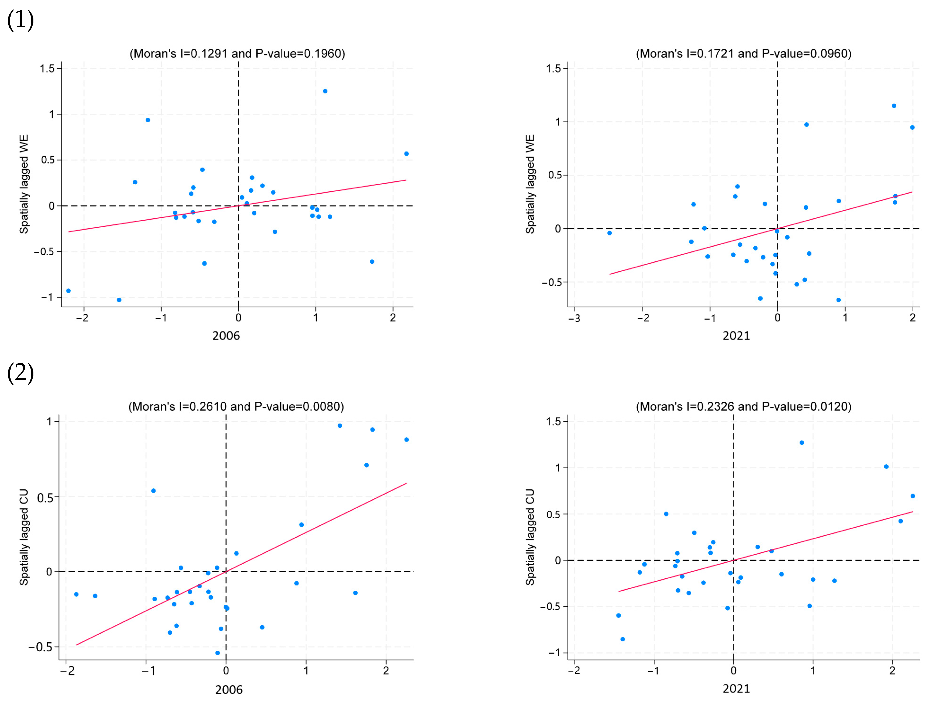
3.5. Spatial Autocorrelation Analysis

During the construction of the spatial econometric model, it is first necessary to test whether the research variables exhibit spatial effects. Moran’s I index is a statistical measure used to assess the degree of spatial clustering among panel members [65]. It can describe the spatial correlation of various phenomena and effectively reflect the similarity of attribute values between spatially adjacent or neighboring units. The value of this index typically ranges between −1 and 1, where values greater than 0 indicate a positive correlation, suggesting that similar observations tend to cluster; values less than 0 indicate negative correlation, implying that dissimilar observations tend to cluster; and values close to 0 suggest no significant spatial clustering trend. This study uses Moran’s I index to determine whether the MSW eco-efficiency exhibits spatial correlation. The general expression for Moran’s I index is as follows:

$$I={\sum }_{i=1}^n{\sum }_{j=1}^n{W}_{ij}\left(x_i-\overline{x}\right)\left(x_j-\overline{x}\right)/S^2{\sum }_{i=1}^n{\sum }_{j=1}^n{w}_{ij}$$

(14)

where $\left(\sum _{i=1}^n{\left(x_i-\overline{x}\right)}^2\right)/n$ represents the sample variance and $w_{ij}$ denotes the elements in the spatial weight matrix. In this study, based on Harke et al. (2022) [66], a spatial distance matrix based on the inverse square of the distance between provinces is used to examine the spatial correlation and heterogeneity of the MSW eco-efficiency. It can be expressed as:

$$w_{ij}\left\{\begin{array}{c}1/d_{ij}^2, i\ne j\\ 0, i=i\end{array}\right.$$

(15)

The value of Moran’s I ranges between −1 and 1. A Moran’s I value greater than 0 indicates a positive spatial correlation for the MSW eco-efficiency, implying high–high clustering or low–low clustering.

3.6. Spatial Econometric Model

Commonly utilized spatial econometric models encompass the spatial lag model (SLM) and the spatial error model (SEM). The former is primarily employed to address issues of spatial dependence, whereas the latter takes into account spatial error correlations. The SDM, building upon the SLM and the SEM, incorporates fixed effects for both time and space, and focuses on the spatial correlation between independent and dependent variables [67]. Incorporating both exogenous and endogenous spatial dependence allows for a comprehensive consideration of the spatial correlation between dependent and independent variables. The specific model formulation is as follows:

$$Y_{it}=\alpha +\rho W{Y}_{ij}+X_{it}\beta +\theta W{X}_{it}+{\mu }_i+{\phi }_t+{\epsilon }_{it}$$

(16)

where $Y_{it}$ is the dependent variable; $X_{it}$ is a vector of independent variables; $\rho$ denotes the spatial autoregressive coefficient; $W$ represents the spatial weight matrix; $\beta$ represents the coefficients of the influencing factors; $\theta$ is the coefficient vector for the spatial lag term; ${\mu }_i$ denotes individual fixed effects, ${\phi }_t$ represents time fixed effects, and ${\epsilon }_{it}$ is the random error term. The parameter $\rho$ is used to measure the interactive characteristics of MSW eco-efficiency. If $\rho >0$, it indicates the existence of a “race to the top” effect in terms of high-quality economic development among cities; conversely, if $\rho <0$, it suggests a “beggar-thy-neighbor” effect in the MSW eco-efficiency among cities.

When spatial spillover effects are present, independent variables not only influence changes in the dependent variable within the same region, but also affect neighboring regions, reflecting spatial interaction. The empirical results of the SDM do not fully capture the spatial relationship between independent and dependent variables. The regression coefficients differ from those obtained through ordinary least squares (OLS) estimation. Le Sage and Pace proposed the partial differential method to decompose the impact of independent variables on dependent variables into direct and indirect effects, and to test for potential spatial spillover effects [68]. The SDM can be rewritten as: $Y={(I-\rho W)}^{-1}+{\left(I-\rho W\right)}^{-1}\left(\beta X+\theta WX\right)+{(I-\rho W)}^{-1}\epsilon$. The partial differential equation matrix form for the k-th explanatory variable in the dependent variable is as follows:

$$\left[\begin{array}{ccc}{\displaystyle \frac{\partial y}{\partial x_{1k}}}& \cdots & {\displaystyle \frac{\partial y}{\partial x_{nk}}}\end{array}\right]=\left[\begin{array}{ccc}{\displaystyle \frac{\partial y_1}{\partial x_{1k}}}& \cdots & {\displaystyle \frac{\partial y_1}{\partial x_{nk}}}\\ ⋮& \ddots & ⋮\\ {\displaystyle \frac{\partial y_n}{\partial x_{1k}}}& \dots & {\displaystyle \frac{\partial y_n}{\partial x_{nk}}}\end{array}\right]={(I-\rho W)}^{-1}\left[\begin{array}{cc}\begin{array}{cc}{\beta }_k& W_{12}{\theta }_k\end{array}& \begin{array}{cc}\cdots & W_{1n}{\theta }_k\end{array}\\ \begin{array}{cc}{W}_{21}{\theta }_k& {\beta }_k\end{array}& \begin{array}{cc}\cdots & W_{2n}{\theta }_k\end{array}\\ \begin{array}{cc}\begin{array}{c}⋮\\ W_{n1}{\theta }_k\end{array}& \begin{array}{c}⋮\\ W_{n2}{\theta }_k\end{array}\end{array}& \begin{array}{cc}\begin{array}{c}\ddots \\ \cdots \end{array}& \begin{array}{c}⋮\\ {\beta }_k\end{array}\end{array}\end{array}\right]$$

(17)

The direct effect corresponds to the average of the diagonal elements in the matrix, representing the direct impact of the explanatory variable on its own dependent variable. The indirect effect corresponds to the average of the off-diagonal elements in the matrix, indicating the influence of the explanatory variable on the dependent variables in surrounding areas. The total effect, which is the sum of the direct and indirect effects, represents the average impact of the local explanatory variable on the dependent variables in all regions. In this paper, we conduct an SDM analysis using panel data, with the aim of investigating the impact of consumption upgrading on MSW eco-efficiency:

$${WE}_{it}={\alpha }_0+\rho W{WE}_{it}+{\delta }_1{CU}_{it}+{\beta }_{1}W{CU}_{it}+{\delta }_2{X}_{it}+{\beta }_{2}W{X}_{it}+{\mu }_i+{\eta }_t+{\epsilon }_{it}$$

(18)

In this model, $t$ represents the study period and $i$ denotes the observed sample. ${WE}_{it}$ presents the technical change in eco-efficiency for region $i$ at time t. $W{WE}_{it}$ is the spatial lag term. The parameters $\rho$ and $\gamma$ represent the influence of adjacent technical changes on the eco-efficiency of region $i$. $W{CU}_{it}$ reflects the effect of adjacent MSWeco-efficiency. $X_{it}$ represents the matrix of control variables, ${\mu }_i$ captures time-fixed effects, and ${\epsilon }_{it}$ is the random error term.

4. Sample Description and Data

4.1. Sample

The empirical application in this study draws its sample from 30 regions across China, including provinces, autonomous regions, and municipalities directly under the central government. The research period spans 2006 to 2021, focusing on areas with population densities ranging from 1250 to 5210 individuals per square kilometer. According to the China National Statistical Yearbook, the nationwide generation of MSW increased from 148.413 million tons in 2006 to 248.692 million tons in 2021, representing a growth rate of 168% [69]. China’s MSW disposal structure is currently transitioning from landfill-based to incineration-based treatment. In 2021, the daily waste treatment capacity reached 1,057,064 tons, with 68.01% incinerated and 24.74% landfilled [70].

Carbon emissions from MSW treatment have risen annually, peaking at 54.3154 million tons in 2018, before declining after 2020 due to the COVID-19 pandemic. Simultaneously, MSW management costs have escalated. In China, urban household waste collection fees are primarily funded by the government and levied on residents through property fees and other channels. From 2011 to 2020, local governments faced a rising deficit between revenues and expenditures [71]. To enhance MSW management performance, local authorities have formulated policies, improved waste disposal facilities, increased investments in recycling technologies, and implemented significant governance changes over the past decade. These factors collectively make China’s MSW a compelling case for investigation.

4.2. Data

The original data for each indicator were sourced from the China Statistical Yearbook, the National Bureau of Statistics website, the Global Statistical Data Analysis Platform, the China Environmental Statistics Yearbook, the China Urban Statistical Yearbook, the China Science and Technology Statistical Yearbook, the China Financial Yearbook, the China Labor Statistical Yearbook, the China Household Survey Yearbook, and the China Urban and Rural Construction Statistical Yearbook. Missing data were supplemented using either the mean imputation method or the exponential smoothing method. Considering that earlier data may have more missing values, errors, or inconsistencies in statistical standards, this study utilized panel data from 30 provinces in China from 2006 to 2021 for empirical analysis.

Table 1. Descriptive statistical results of variables.

Variables	Unit	Mean	Minimum	Maximum	Standard Deviation
Garbage Collection (GC)	10,000 tons	627.74	50.9	3347.3	486.94
Workforce (WME)	10,000 people	7.95	0.80	21.70	3.95
Waste Treatment Investment (INV)	100 million RMB	71.18	0.01	973.04	121.49
Solid Waste Treatment Capacity (WTC)	100 tons per day	187.35	4.00	1767.36	187.96
Waste Treatment (WT)	10,000 tons	592.27	59.15	3345.77	480.74
Greenhouse Gas Emissions (GHGs)	10,000 tons	142.54	9.72	803.26	108.78
Waste Eco-efficiency (WE)	/	0.41	0.11	1.16	0.20
Consumption Updating (CU)	/	−1.54	−3.53	−0.08	0.68
Educational Year (EY)	/	2.19	1.89	2.55	0.11
Dependency Ratio (DR)	/	0.38	0.19	0.58	0.07
Dependence on Foreign Trade (FT)	/	−1.34	−4.51	0.89	0.98
Pollution Control (PC)	/	2.80	0.04	20.35	2.56
ER		0.21	0.08	0.54	0.10
Infrastructure Level (INF)	/	3.57	2.12	4.46	0.41
Economic Level (GDP)	/	4.54	3.76	5.26	0.28
Population Density (PD)	/	0.46	−2.96	−0.55	0.46
Industrial Agglomeration (IA)	/	−2.39	−4.75	−1.12	0.55
Regional innovation index (RI)	/	1.44	0.82	1.53	0.09

provides descriptive statistics for all variables. The dataset consists of two parts: the first part is used for calculating MSW eco-efficiency and technological changes via the SSBM-DEA model, while the second part is prepared for the SDM to analyze the impact of policies on technological progress. Moreover, all monetary data were deflated using price indices, and all variables were transformed using natural logarithms.

4.2.1. Variables for the Super SBM-DEA Model

Existing studies often measure eco-efficiency by increasing desirable outputs while decreasing undesirable outputs and conserving resources. However, due to differences in resource endowments, market environments, and technological barriers, technical heterogeneity exists among different DMUs. This study constructs a SSBM-DEA model to estimate the MSW eco-efficiency and incorporates GHGs as undesirable outputs into the model.

(1)

Input Variables

Referring to the indicators proposed by Zhang et al. [72] and Puertas et al. [73], and considering data availability, this study selects the following input indicators:

• Solid Waste Generation: MSW primarily includes residential waste, street cleaning waste, and institutional waste. This study uses the volume of solid waste collected and transported to represent MSW generation. The collection volume includes waste transported via sealed vehicles (or containers), reflecting the current state of waste collection in a region;
• Labor Input: Many scholars, based on the Cobb-Douglas production function, consider labor as a fundamental input indicator. This study uses the number of employees in urban units within the water conservation, environmental, and public facility management sectors as a proxy for labor input;
• Capital Input: Solid waste treatment investment is used as a representative of capital input. Specifically, this study considers investments in urban household waste treatment as a measure of eco-efficiency input proposed by Du et al. [74];
• Harmless Treatment Capacity: The capacity for harmless treatment of solid waste reflects the performance of waste treatment infrastructure [75]. Therefore, this study also includes the harmless treatment capacity of solid waste as an input variable.

(2)

Output Variables

Based on the principles of minimization and harmlessness in urban household waste management, the study selects solid waste treatment volume as the desirable output variable and greenhouse gas emissions as the undesirable output variable.

• Solid Waste Treatment Volume: The volume of harmlessly treated household waste reflects the current state of harmless treatment. This study uses the harmless treatment volume of MSW to represent the waste treatment situation in different regions.
• Greenhouse Gas Emissions: From an environmental perspective, GHGs are an important indicator for evaluating waste treatment efficiency. This study uses the calculated GHGs as the undesirable output to measure the eco-efficiency of MSW [12].

4.2.2. Variables for the Consumption Upgrade Evaluation System

This study uses the entropy method to determine the weight of the consumption upgrade indicators. Building on previous research [76], the perspective of consumption sustainability is added, and the consumption upgrade is measured from three aspects: consumption level upgrade, consumption structure upgrade, and green consumption upgrade. The specific indicators selected are shown in

Table A4. Descriptive statistics of the variables.

Variable	Mean	Standard Deviation	Max	Min	Variable	Mean	Standard Deviation	Variable	Mean
Consumer Price Index	1.90	2.66	24.81	1.00	Mobile Phone Penetration Rate	85.89	33.18	189.50	17.40
Innovation Product Supply	2.79	3.28	27.18	0.17	Per Capita Postal and Telecommunication Volume	3297.26	3299.39	17,583.00	581.28
Digital Consumption Environment	0.36	0.27	1.07	0.02	Digital Consumption Level	0.15	0.16	0.80	0.01
Logistics Conditions	0.26	0.22	2.23	0.00	Proportion of Clean Energy Consumption	0.15	0.06	0.79	0.07
Per Capita Consumption Level	66,680.46	77,228.04	395,894.39	4823.25	Wastewater Emissions	25.12	7.28	66.61	7.99
Regional Consumption Capacity	1.82	1.21	7.26	0.19	Air Emissions	88.27	95.89	647.06	0.11
Final Consumption Rate	51.17	8.35	80.00	32.08	Green Travel	11.91	3.24	26.55	5.73
Income Scale	19,904.72	12,381.46	78,026.60	2715.85	Waste Treatment	85.05	19.38	100.00	17.80
Unemployment Rate	3.39	0.66	5.10	1.20	Green Cover	38.52	4.44	55.10	23.45
Higher Education Enrollment Rate	8.39	5.19	26.86	0.36	Road Sweeping Area	22,413.82	20,476.06	132,135.00	1367.00
Labor Force Proportion	0.62	0.07	0.81	0.42	Per Capita Park Green Area	12.03	3.15	21.05	5.49
Average Consumption Propensity	1.02	0.25	2.52	0.60	Sewage Treatment	0.84	0.16	1.00	0.20
Clothing Consumption Proportion	0.09	0.03	0.16	0.04	Environmental Investment	0.01	0.01	0.03	0.00
Housing Consumption Proportion	0.16	0.07	0.41	0.07	Industrial Solid Waste Utilization	6097.56	4909.13	25,230.00	113.00
Education and Culture Consumption Proportion	0.12	0.02	0.17	0.07	Forest Area	33.65	17.99	66.80	4.00
Daily Goods and Services Consumption Proportion	0.06	0.01	0.09	0.04	Financial Situation	28,550.78	29,357.20	195,680.62	729.83
Transport and Communication Consumption Proportion	0.13	0.02	0.21	0.09	Government Support	0.23	0.10	0.64	0.08
Medical Care Expenditure Proportion	0.08	0.02	0.14	0.04	Urbanization Level	56.37	13.70	89.60	27.46
Other Goods and Services Consumption Proportion	0.03	0.01	0.06	0.02	Social Security Fiscal Expenditure	0.13	0.04	0.31	0.02
Engel’s Coefficient	0.58	0.03	0.67	0.49	Medical Insurance Participation Rate	0.54	0.33	1.34	0.07
Natural Gas Penetration Rate	0.92	0.09	1.14	0.57	Medical Services	4.79	1.51	8.34	1.60

in Appendix A.

4.2.3. Control Variables for the SDA Model

To select potential exogenous variables influencing the eco-efficiency scores of MSW management, three criteria were considered: the characteristics of solid waste management in China, the availability of information for the assessed provinces, and existing literature. The following variables were taken into account:

Education Level (EY). Sociodemographic factors exert multifaceted influences on the generation of MSW. Individuals with higher levels of education are more likely to engage in waste sorting and recycling behaviors [77]. In this study, a weighted approach based on educational attainment duration is adopted to calculate the average years of education per capita.

Demographic shifts have emerged as a significant factor influencing current consumption levels and constraining economic development. The aging of the population structure tends to decrease overall household consumption levels. An increase in the proportion of elderly individuals within households leads to a decline in total household consumption while elevating expenditure on family development. Conversely, an increase in the proportion of young children in households promotes the optimization and upgrading of household consumption, enhancing both subsistence and development-oriented consumption, which in turn affects the generation of solid waste [78]. In this study, the dependency ratio (DR), defined as the proportion of non-working population to the total population, is employed as a variable representing demographic structure.

The degree of dependence on foreign trade reflects a country’s economic reliance on international commerce. The environmental impact of foreign trade manifests not only in the transfer of environmental pollution among countries with different endowments and income levels, but also in changes to the structure of exported products [79]. In this study, the ratio of imports and exports to GDP is utilized to measure the degree of foreign trade dependence (FT).

Pollution control (PC) represents the regulatory measures implemented by governments to limit pollutant emissions. It reflects the relative relationship between investments in industrial pollution control and the development of the secondary industry (primarily industrial) within a specific economic system [80]. In this paper, pollution control is represented by the ratio of industrial pollution investment to the output value of the secondary industry.

Economic Level (GDP). Existing research indicates that the level of regional economic development is a crucial factor influencing environmental quality. Studies have shown that economic growth has promoted the generation of municipal solid waste, such that, at the current stage, development levels have not yet achieved a decoupling effect on the production of municipal solid waste, and instead exhibit an expanding nexus state [81]. In this study, the natural logarithm of the gross domestic product (GDP) of the municipal district in the current year is used to measure the local level of economic development.

Industrial Agglomeration (IA). Underdeveloped regions often neglect environmental issues in pursuit of regional economic development, thereby becoming pollution havens for developed regions. Most studies use location quotient or the ratio of the value-added of the secondary industry to the region’s gross domestic product (GDP), divided by the ratio of the national value-added of the secondary industry to the national GDP, to calculate industrial agglomeration [38,82,83]. However, these methods only consider the situation in manufacturing or certain industries. In this paper, the level of industrial agglomeration is measured by the ratio of urban employed personnel to urban area.

The level of infrastructure (INF) serves as the foundation for the normal operation of cities, acting as the carrier for household consumption and solid waste management, and constitutes the cornerstone of urban development. The level of infrastructure has emerged as a significant factor influencing ecological management efficiency. In this paper, we select the per-capita road area as a metric to assess the level of regional infrastructure.

Human activities generate waste and contribute to environmental pollution. An increase in population leads to a cumulative increase in the production of solid waste [84]. In this paper, we use the number of people per unit area within a region as an indicator of population density (PD) to measure the population effect on waste management.

The enhancement of regional innovation capability can significantly promote the innovation and application of waste management technologies, thereby optimizing waste processing procedures, increasing resource recovery and utilization rates, and reducing the risk of environmental pollution [85]. In this paper, the China Regional Innovation and Entrepreneurship Index (RI) is selected as a proxy indicator for regional innovation capability [86].

5. Results and Discussions

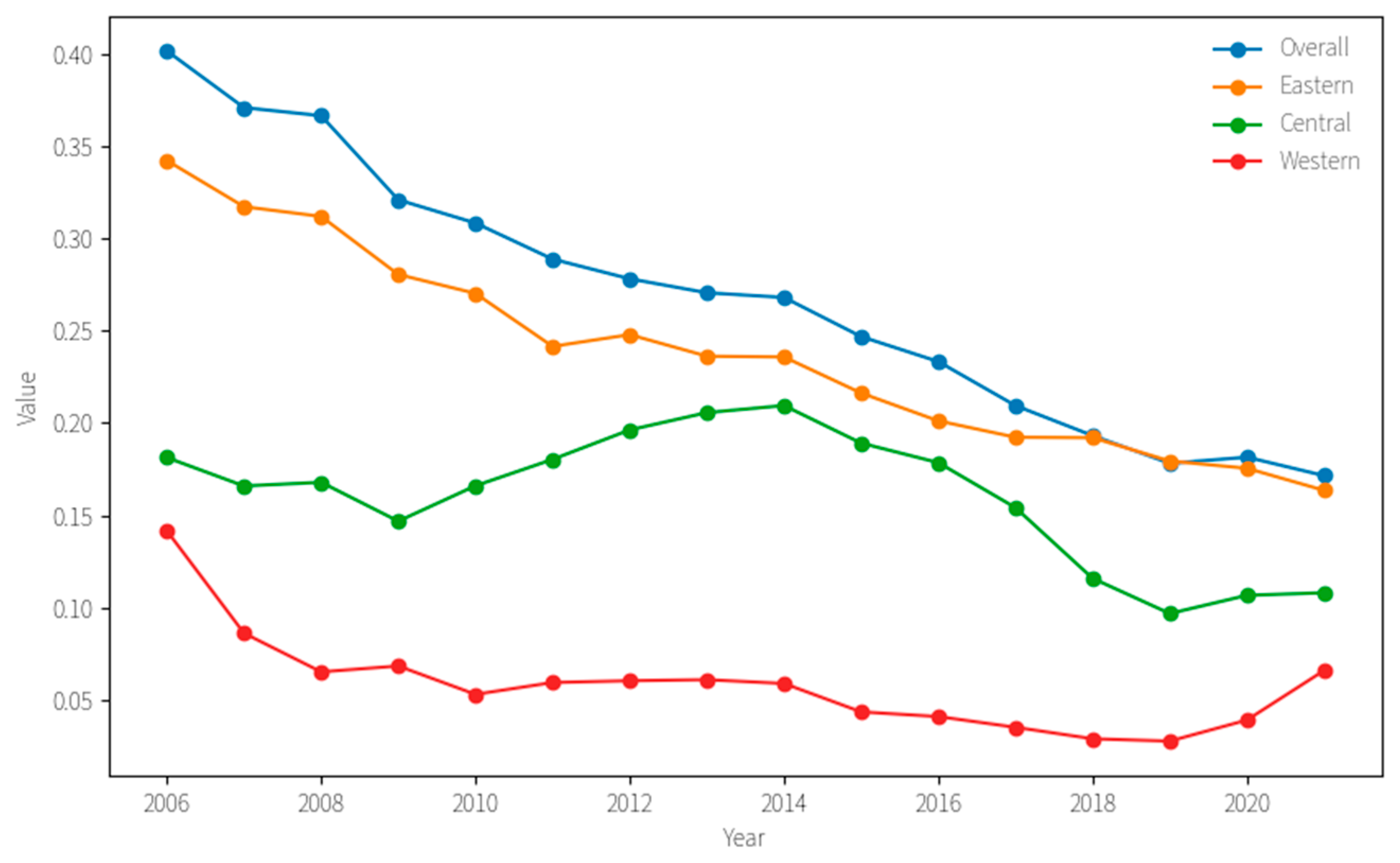
5.1. Regional Differences in CU in China

In order to explore the regional differences in CU in China, the 30 provinces of China are divided into eastern, central, and western regions. The Dagum Gini coefficient is used to calculate and decompose CU. Figure 1 presents the Gini coefficient results at the national and regional levels from 2006 to 2021.

According to the calculation results, the Gini coefficients of CU in all regions of China during the observation period were below 0.4. With the exception of the central region, the overall, eastern, and western regions exhibited a similar trend in the evolution of their Gini coefficients, showing a downward trajectory. This indicates that the issue of unequal distribution of CU across regions is converging, with the CU gap narrowing over time. Specifically, the national Gini coefficient showed a downward trend during the study period, dropping from 0.40 to 0.17, a decrease of 0.23.

From a regional perspective, the eastern region had the highest average Gini coefficient of 0.24, indicating the greatest degree of regional differentiation. The western region, on the other hand, had the lowest average of 0.06, showing the least degree of differentiation. The central region experienced a brief increase in the Gini coefficient between 2009 and 2014, followed by a decline.

A subgroup decomposition of the Dagum Gini coefficient for the CU indicator can further reveal the regional differences and dynamic changes in the CU of Chinese residents. Through this decomposition, the regional disparity of CU can be broken down into intra-regional disparities, inter-regional disparities, and super-change density. The decomposition helps in identifying the sources of these regional disparities and the evolving trends in their contribution rates (see

Table 2. Decomposition results of Gini coefficient.

Year	Overall	Intra-Regional Difference			Inter-Regional Difference			Contribution Rate
		Eastern	Central	Western	Eastern and Central	Eastern and Western	Central and Western	Intra-Regional	Inter-Regional	Super-Variation Density
2006	0.40	0.34	0.18	0.14	0.47	0.56	0.22	26.70	69.05	4.25
2007	0.37	0.32	0.17	0.09	0.46	0.51	0.16	25.95	70.45	3.60
2008	0.37	0.31	0.17	0.07	0.47	0.50	0.15	25.61	70.66	3.73
2009	0.32	0.28	0.15	0.07	0.45	0.45	0.13	25.57	70.53	3.90
2010	0.31	0.27	0.17	0.05	0.40	0.42	0.13	25.59	69.33	5.08
2011	0.29	0.24	0.18	0.06	0.37	0.40	0.14	24.97	68.00	7.03
2012	0.28	0.25	0.20	0.06	0.34	0.38	0.16	26.50	64.52	8.98
2013	0.27	0.24	0.21	0.06	0.33	0.36	0.16	26.36	63.57	10.07
2014	0.27	0.24	0.21	0.06	0.32	0.36	0.17	26.57	62.76	10.67
2015	0.25	0.22	0.19	0.04	0.30	0.34	0.15	25.90	63.89	10.21
2016	0.23	0.20	0.18	0.04	0.28	0.32	0.15	25.43	64.47	10.09
2017	0.21	0.19	0.15	0.04	0.26	0.28	0.12	25.98	64.32	9.70
2018	0.19	0.19	0.12	0.03	0.24	0.27	0.10	26.25	66.60	7.15
2019	0.18	0.18	0.10	0.03	0.22	0.26	0.08	25.89	67.91	6.20
2020	0.18	0.18	0.11	0.04	0.22	0.26	0.10	25.81	66.20	7.99
2021	0.17	0.16	0.11	0.07	0.17	0.25	0.14	26.71	64.65	8.64

). According to the decomposition results, the structure of the sources of regional differences in various consumption expenditure indicators is quite similar, with inter-regional differences being the primary source of disparity. Throughout the study period, the contribution of inter-regional differences to the regional disparity of CU indicators consistently exceeded that of intra-regional differences and super-change density, with contributions always surpassing 50%, albeit fluctuating downward. Among the regions, the largest inter-regional differences were found between the eastern and western regions, with an average contribution value of 0.37. The smallest inter-regional differences were between the central and western regions, with an average contribution value of 0.14. The contribution rate of super-change density was the smallest, showing an overall upward-then-downward trend, fluctuating between 3.60% and 10.67%.

5.2. MSW Eco-Efficiency Spatio-Temporal Pattern

Using the global Moran’s I index and based on the spatial geographic weight matrix, the global spatial correlation of MSW eco-efficiency and CU from 2006 to 2011 was examined. The specific results are shown in

Table 3. Global spatial correlation test results.

Year	WE		CU
	I	p	I	p
2006	0.13	0.03	0.62	0.00
2007	0.17	0.03	0.30	0.00
2008	0.02	0.13	0.31	0.00
2009	0.02	0.11	0.30	0.00
2010	0.14	0.06	0.31	0.00
2011	0.04	0.16	0.29	0.00
2012	0.18	0.04	0.27	0.00
2013	0.17	0.05	0.25	0.00
2014	−0.05	0.85	0.22	0.01
2015	−0.05	0.91	0.23	0.01
2016	0.16	0.04	0.22	0.01
2017	0.17	0.06	0.23	0.01
2018	0.10	0.06	0.24	0.00
2019	0.11	0.10	0.27	0.00
2020	0.28	0.00	0.23	0.01
2021	0.28	0.00	0.23	0.01

, where the first column under each variable represents the global Moran’s I value and the second column indicates the corresponding p-value.

Overall, during the study period, the global Moran’s I index for MSW eco-efficiency was positive in most years and passed the test at the 10% confidence level. This indicates a significant positive spatial correlation of eco-efficiency overall, showing characteristics of spatial aggregation. The eco-efficiency of adjacent provinces exhibited a significant correlation, with a positive feedback effect between provinces. In 2008, 2009, 2011, 2014, and 2015, the Moran’s I values were not significant, and negative values were observed in 2014 and 2015. This suggests that the spatial correlation of eco-efficiency was not prominent during these years. From the perspective of Moran’s I values, there was a general upward trend throughout the study period, indicating that the spatial correlation of eco-efficiency gradually strengthened and consistently exhibited a positive correlation.

CU was significant at the 1% confidence level throughout the study period, with a mean value of 0.28. This indicates a high level of spatial positive correlation in CU, showing a clear trend of positive spatial aggregation. Between 2006 and 2011, the Moran’s I values first decreased, then increased, and then decreased again, with turning points in 2015 and 2020. This suggests that CU exhibited alternating patterns of strong and weak positive spatial correlation.

To further examine the spatial autocorrelation of MSW eco-efficiency and CU in China and better reveal their spatial distribution, this study further calculated the local Moran’s I index. The local spatial autocorrelation index was employed to analyze spatial clustering and its temporal variations. They were divided into four quadrants: the first quadrant represented high–high (H–H) clustering, indicating high technical efficiency of DMUs; the third quadrant, low–low (L-L) clustering; the second quadrant, low–high (LH) clustering, where DMUs with lower TC were surrounded by those with higher TC; and the fourth quadrant, the opposite situation (H-L). A positive slope signified positive spatial correlation, whereas a negative slope indicated the opposite [87]. Due to space limitations, scatter plots of Moran’s I indices for MSW eco-efficiency (1) and CU (2) for the years 2006 and 2021 are presented in Figure 2. The Moran’s I index values for MSW eco-efficiency are clustered in the first and third quadrants, indicating a clear spatial aggregation. Compared with 2006, the overall trend of the Moran’s I indexes in 2021 shifted from dispersion to concentration. Similarly, the CU observations were also clustered in the third quadrant, with the overall trend becoming more concentrated. The spatial dependence type in the third quadrant was L-L, which suggested that cities with lower MSW eco-efficiency exhibited geographical clustering. In contrast, cities in the first quadrant showed H-H spatial dependence.

5.3. Analysis of the Impact of CU on MSW Eco-Efficiency

This study conducts an SDM by distinguishing between time-lag effects, spatial-lag effects, and spatiotemporal-lag effects. After exploring the significant spatial dependence of MSW eco-efficiency during the study period, this section further investigates the appropriate spatial panel regression model. To obtain objective results, we first conducted several tests to select the appropriate model. We used the Lagrange multiplier (LM) and robust Lagrange multiplier (Robust LM) to test the conventional panel data model without spatial interaction effects, and examined the spatial correlation of the model’s regression residuals in order to determine the basic form of the spatial panel regression model.

Table 4. Spatial econometric model testing.

Test		WE	p
LM test	LM-error	7.09	0.01
	Robust LM-error	14.73	0.00
	LM-lag	1.94	0.16
	Robust LM-lag	9.57	0.00
LR test	LR-SDM/SAR	37.22	0.00
	LR-SDM/SEM	42.28	0.00
Wald test	Wald-SDM/SAR	38.17	0.00
	Wald-SDM/SEM	43.07	0.00
Spatial-temporal fixed effects test	Lrtest-id-both	67.82	0.00
	Lrtest-time-both	739.13	0.00

reports the test results for the selection of spatial econometric models. First, except for LM-Lag, the results of the Robust LM-Lag, LM-Error, and Robust LM-Error tests all passed the 1% significance level, indicating that a spatial econometric model can be selected for empirical analysis. Secondly, the LR likelihood ratio test shows that the test statistics passed the 1% significance level, suggesting that the SDM model cannot degenerate into the SAR or SEM models. The Wald test statistics are also significant at the 1% level, indicating that the SDM is more suitable for empirical analysis than the SAR model or the SEM. Next, tests for individual and time effects were conducted. According to the joint significance test results, both the double-fixed time effect test and the double-fixed individual effect test were significant at the 1% level, rejecting the null hypothesis. This implies that the double-fixed effect SDM should be chosen. Additionally, the Hausman statistic for MSW eco-efficiency was 92.88, which passed the 1% significance level test, thus rejecting the null hypothesis and selecting the fixed effects model.

The regression results of the impact of CU on the MSW eco-efficiency are shown in

Table 5. Benchmark regression results.

	(1)	(2)	(3)	(4)	(5)	(6)
	Ind	Time	Both	Wx-Ind	Wx-Time	Wx-Both
CU	0.359 ***	0.321 ***	0.332 ***	−0.118	0.429 ***	0.349 **
	(−6.490)	(−6.850)	(−6.360)	(−1.11)	(−3.310)	(−2.650)
EY	−0.114	2.101 ***	0.134	0.268	1.092	0.145
	(−0.30)	(−8.210)	(−0.360)	(−0.480)	(−1.580)	(−0.170)
FT	−0.0728 *	−0.122 ***	−0.0637 *	−0.078	0.100	−0.224 **
	(−2.29)	(−4.77)	(−2.14)	(−1.250)	−1.300	(−2.820)
ER	0.017	0.022	0.004	0.0512 *	−0.069	−0.032
	(−1.200)	(−1.250)	(−0.320)	(−2.160)	(−1.62)	(−0.99)
DR	−0.208	0.266 *	−0.184	0.041	0.435	0.806 *
	(−1.55)	(−2.230)	(−1.42)	(−0.210)	(−1.440)	(−2.390)
INF	0.073	−0.996 ***	0.175 *	1.209 ***	0.122	−0.217
	(−0.970)	(−21.000)	(−2.370)	(−6.530)	(−0.760)	(−0.940)
GDP	0.413	0.139	−0.677	1.093 *	−1.327 **	3.954 ***
	(−1.120)	(−0.910)	(−1.780)	(−2.540)	(−3.280)	(−4.580)
PD	0.020	−0.155 **	0.033	0.333 *	−0.032	0.629 ***
	(−0.390)	(−2.79)	(−0.670)	(−2.360)	(−0.21)	(−4.400)
IA	0.055	0.019	−0.027	−0.312 **	−0.315 *	−0.871 ***
	(−1.180)	(−0.420)	(−0.60)	(−2.61)	(−2.04)	(−5.41)
RI	0.048	−0.144	0.027	0.141	0.245	0.046
	(−0.390)	(−0.790)	(−0.230)	(−0.580)	(−0.580)	(−0.170)
rho	0.406 ***	0.101	0.0664 *
	(−6.840)	(−1.310)	(−0.910)
sigma2	0.0250 ***	0.0557 ***	0.0215 ***
	(−15.320)	(−15.480)	(−15.480)
Individual fixed	Yes	No	Yes
Time fixed	No	Yes	Yes
R2	0.118	0.506	0.064
N	480	480	480

Notes: Asterisks indicate the significance level, and the number of asterisks indicates the significance level size. ***, **, and * indicate statistical significance at 1%, 5%, and 10%, respectively. The significance of all the tables below is consistent with this.

. Columns (1), (2), and (3) represent the results with individual fixed effects, time fixed effects, and dual fixed effects, respectively. The regression coefficient of 0.33 and the spatial lag term of 0.35 are both positive and pass the significance test at the 1% confidence level. This indicates that the transformation of eco-efficiency can significantly improve the MSW eco-efficiency within the region, and there is a significant spatial correlation effect. Neighboring cities exhibit a “demonstration effect”, meaning that the improvement in eco-efficiency in one city positively influences the levels of its neighboring cities. This is similar to the findings of Zhao et al. [52], reinforcing the premise that regional synergies and collaborative environmental strategies can amplify the efficacy of waste management practices.

It is imperative to consider the underlying mechanisms that facilitate this spatial correlation. Potential factors may include the diffusion of innovative waste management technologies, shared environmental policies, and inter-city collaborations aimed at sustainability. Additionally, the role of socio-economic factors and public awareness in driving eco-efficiency improvements warrants exploration.

Given the existence of spatial lag terms in the SDM and the inclusion of global spatial effects in the model specification, the estimation results cannot directly reflect the marginal effects of individual variables. To precisely capture the spatial spillover effects of various variables, further decomposition of the spatial effects is required. This enables an in-depth exploration of the spatial interactions of CU and other influencing factors. The decomposition of spatial effects for the MSW eco-efficiency is presented in

Table 6. Analysis of the spatial effect decomposition.

	Direct	Indirect	Total		Direct	Indirect	Total
CU	0.336 ***	0.395 **	0.730 ***	INF	0.173 *	−0.217	−0.044
	−0.052	−0.145	−0.132		−0.069	−0.244	−0.254
EY	0.096	0.119	0.215	GDP	−0.710 *	−4.159 ***	−4.869 ***
	−0.323	−1.044	−1.133		−0.349	−0.875	−0.955
FT	−0.0637 *	−0.250 ***	−0.313 ***	PD	0.031	0.678 ***	0.709 ***
	−0.031	−0.074	−0.072		−0.044	−0.136	−0.147
ER	0.005	−0.027	−0.022	IA	−0.032	−0.961 ***	−0.993 ***
	−0.015	−0.033	−0.038		−0.035	−0.156	−0.164
DR	−0.206	0.843 *	0.636	RI	0.025	0.054	0.079
	−0.149	−0.375	−0.410		−0.121	−0.313	−0.261
rho	0.0664 *			sigma2	0.0215 ***
	−0.073				−0.001
Fixed effect	Yes	Yes	Yes	R2	0.064	R2	0.064

Notes: Asterisks indicate the significance level, and the number of asterisks indicates the significance level size. ***, **, and * indicate statistical significance at 1%, 5%, and 10%, respectively. The significance of all the tables below is consistent with this.

.

Both the direct and indirect effects of CU on the MSW eco-efficiency are significantly positive at the 1% level. This demonstrates that CU not only significantly enhances local MSW eco-efficiency, but also generates substantial spatial spillover effects through the flow of resources, technologies, and knowledge, thereby improving waste management efficiency in neighboring regions. The advancement in the level of CU fosters higher-level consumption patterns, which, in turn, transforms industrial structures. On the one hand, changes in demand reduce solid waste generation and improve treatment efficiency, thereby objectively enhancing the MSW eco-efficiency. On the other hand, the cross-regional flow of innovative resources and industrial clustering accelerates, creating spatial spillover effects on surrounding regions. The spatial spillover effects suggest that neighboring regions can benefit from shared technologies, policies, and infrastructure investments. For instance, the central and western regions can leverage their latecomer advantages in technology. Establishing regional waste management networks, promoting knowledge exchange, and coordinating policies could amplify these benefits.

While CU promotes higher-level consumption patterns, it may also lead to increased waste generation, particularly from the disposal of new products and packaging. But reducing the generation of MSW with a high carbon content at its source is the fundamental solution to reducing emissions [54]. This could strain existing waste management systems and offset some of the gains in eco-efficiency. Addressing these challenges requires proactive measures, such as promoting circular economy practices, encouraging product design for durability and recyclability, and implementing extended producer responsibility (EPR) policies [88].

For CU, the direct effect is 0.34, indicating that a 1% increase in the level of CU improves the local MSW eco-efficiency by 0.34%. The indirect effect is 0.40, suggesting that it leads to a 0.40% improvement in the MSW eco-efficiency in neighboring areas. The indirect effect is slightly higher than the direct effect, which highlights the significant role of spatial spillover effects caused by the flow of various elements associated with CU in enhancing the MSW eco-efficiency of other regions. This suggests that the spatial spillover effects driven by the flow of resources, knowledge, and technologies associated with CU play a critical role in amplifying eco-efficiency gains across regions. The slightly higher indirect effect highlights the interconnectedness of urban systems and the potential for collaborative regional strategies to achieve broader environmental benefits.

From the perspective of influencing factors, infrastructure shows a significant positive effect in the regression results, but is not significant in the indirect and total effects. Previous research has reached a consensus on this point. For example, Shigemi et al. revealed the location-based advantages and regional technological differences in waste treatment activities [89]. This aligns with real-world economic and social conditions, as improvements in infrastructure significantly enhance local MSW equipment and technology, but do not have a notable impact on neighboring areas. However, the lack of significance in indirect and total effects suggests that infrastructure advancements primarily benefit the immediate region without substantially impacting neighboring areas. This underscores the localized nature of infrastructure-driven improvements and the need for targeted investments in underdeveloped regions to ensure equitable progress.

In contrast, trade dependency, industrial agglomeration, and economic development levels exert a significant negative effect on the MSW eco-efficiency. This indicates that trade activities, industrial clustering, and economic growth place substantial pressure on waste management departments, increasing the difficulty of environmentally sound waste treatment, decreasing pollution, and ultimately decreasing eco-efficiency. These factors likely lead to higher waste generation and resource consumption, ultimately lowering eco-efficiency. This finding calls for a reevaluation of economic and industrial policies to integrate sustainability goals, such as promoting circular economy practices and reducing waste generation at the source.

Interestingly, population density and dependency ratios demonstrate a significant positive influence on MSW eco-efficiency in terms of indirect effects. This suggests that higher population density and dependency ratios may foster greater efficiency in waste management practices, possibly due to economies of scale or increased public awareness and participation in waste reduction initiatives. These findings highlight the potential for leveraging demographic factors to enhance eco-efficiency, particularly in densely populated urban areas.

The results emphasize the dual importance of local initiatives and regional collaboration in improving MSW eco-efficiency. While infrastructure development and localized CU efforts are crucial, the spatial spillover effects of CU and the influence of demographic factors offer additional pathways for enhancing waste management practices. Conversely, the negative impacts of trade dependency, industrial agglomeration, and economic growth underscore the need for integrated policies that balance economic development with environmental sustainability. Future research could explore the mechanisms driving these spatial spillover effects and the role of policy interventions in mitigating the adverse impacts of economic activities on waste management systems

5.4. Robustness Tests

(1)

Replacing the Spatial Weight Matrix

To further ensure the robustness of the model results, this study replaced the spatial geographic matrix with a spatial adjacency matrix, spatial economic distance matrix, and spatial economic–geographic weighted distance matrix to verify the reliability of the SDM.

Table 7. Regression results of the CU composite index with the replacement of the spatial weight matrix.

	(1)	(2)	(3)	(4)	(5)	(6)
CU	0.410 ***	0.365 ***	0.421 ***	0.048	−0.161	−0.030
	−0.054	−0.059	−0.060	−0.103	−0.129	−0.120
EY	0.100	−0.461	−0.258	−0.291	0.740	1.055
	−0.388	−0.396	−0.393	−0.855	−0.928	−0.846
FT	−0.0996 ***	−0.122 ***	−0.123 ***	0.029	0.152 *	0.155 *
	−0.030	−0.031	−0.030	−0.053	−0.076	−0.071
ER	−0.001	0.001	−0.003	−0.037	−0.051	−0.0782 *
	−0.014	−0.014	−0.014	−0.029	−0.034	−0.032
DR	0.022	0.089	0.092	−0.269	0.828 **	0.911 ***
	−0.136	−0.137	−0.137	−0.259	−0.311	−0.275
INF	0.017	−0.017	−0.017	−0.430 *	0.299	−0.116
	−0.079	−0.079	−0.077	−0.203	−0.226	−0.218
GDP	−0.409	−1.292 ***	−1.204 **	−2.361 **	1.074	−1.477
	−0.395	−0.385	−0.381	−0.760	−0.999	−0.846
PD	0.090	0.147 **	0.119 *	0.341 **	−0.244 **	−0.156 *
	−0.049	−0.051	−0.050	−0.122	−0.078	−0.077
IA	−0.018	−0.113 *	−0.078	−0.013	−0.119	−0.176 *
	−0.045	−0.052	−0.049	−0.119	−0.076	−0.074
RI	−0.038	0.029	0.003	0.238	0.304	0.205
	−0.108	−0.098	−0.096	−0.182	−0.207	−0.195
rho	0.277 ***	0.076	0.129 *
	−0.057	−0.069	−0.066
sigma2	0.0227 ***	0.0242 ***	0.0239 ***
	−0.001	−0.002	−0.002
Fixed effect	Yes	Yes	Yes
N	480	480	480
R2	0.043	0.089	0.023

Notes: Asterisks indicate the significance level, and the number of asterisks indicates the significance level size. ***, **, and * indicate statistical significance at 1%, 5%, and 10%, respectively. The significance of all the tables below is consistent with this.

present the regression results of CU indicators on the MSW eco-efficiency after replacing the spatial weight matrix. Columns (1) and (4) represent the spatial adjacency matrix, columns (2) and (5) represent the spatial economic distance matrix, and columns (3) and (6) represent the spatial economic-geographic weighted distance matrix.

According to

Table 8. Robustness test under time-lag effect.

	(1)	(2)	(3)	(4)
	Lagged One Period	Lagged One Period	Lagged Two Period	Lagged Two Period
WE_1	0.677 ***	0.671 ***	0.624 ***	0.613 ***
	−0.040	−0.028	−0.072	−0.046
WE_2			0.061	0.061
			−0.061	−0.042
CU	0.055		0.040
	−0.050		−0.051
Control variables	Yes	Yes	Yes	Yes
Individual Fixed	Yes	Yes	Yes	Yes
Time Fixed	Yes	Yes	Yes	Yes
rho	0.155 ***	0.016 ***	0.161 ***	0.024 ***
	−0.034	−0.064	−0.034	−0.064
sigma2	0.012 ***	0.011 ***	0.012 ***	0.011 ***
	−0.002	−0.001	−0.002	−0.001

Notes: Asterisks indicate the significance level, and the number of asterisks indicates the significance level size. *** indicates statistical significance at 1%. The significance in all the tables below is consistent with this.

, even after replacing the weight matrix, the impact of CU remains significant and passes the 1% significance level test, showing a positive effect. This indicates that CU in the region has a positive and significant effect on improving the eco-efficiency of local MSW. Except for the spatial economic distance matrix, spatial lag effects are observed in all cases, and the regression results remain valid.

(2)

Time Lag Effect

To further verify the stability of the model, a multi-period lag regression was applied to the SDM. As shown in

Table 9. Regional heterogeneity test.

WE	Eastern Region	Central Region	Western Region	Delete Municipalities
CU	−0.135	0.289 ***	0.214 **	0.428 ***
	(−1.48)	(3.77)	(2.59)	(8.51)
CVs	Yes	Yes	Yes	Yes
WX	Yes	Yes	Yes	Yes
rho	−0.337 ***	0.252 **	−0.237 *	0.375 ***
	(0.78)	(3.11)	(−2.22)	(5.86)
sigma2	0.0134 ***	0.0059 ***	0.0191 ***	0.0174 ***
	(9.71)	(8.44)	(8.42)	(14.42)
Fixed effect	Yes	Yes	Yes	Yes
N	192	144	144	416
R2	0.0273	0.317	0.512	0.0255

Notes: Asterisks indicate the significance level, and the number of asterisks indicates the significance level size. ***, **, and * indicate statistical significance at 1%, 5%, and 10%, respectively. The significance in all the tables below is consistent with this.

, the MSW eco-efficiency with a one-period lag was significantly positive at the 1% level, indicating that the development of eco-efficiency in the previous period had a significant promoting effect on its development in the subsequent period. However, the eco-efficiency with a two-period lag was not significant. Across the regression results from one-period to two-period lags, the regression coefficients of CU variables were not significant at the 10% significance level. This finding partially suggests that the model demonstrated good stability. The spatial autocorrelation coefficient (rho) for lagged periods was significant at the 1% level, indicating that the local eco-efficiency of waste management exerted a significant spatial effect on the waste management in other regions.

5.5. Heterogeneity Tests

The aforementioned results indicate that CU exhibited a significant promotional effect on the MSW eco-efficiency. However, regarding cities of varying sizes, a consistent conclusion regarding the impact of CU on MSW eco-efficiency cannot be drawn. Based on administrative regional divisions, this study categorized 30 regions in China into eastern, central, and western areas, and conducted a test for regional heterogeneity among them. Next, owing to the unique administrative status and economic significance of municipalities directly under the central government, this study excluded four such municipalities (specifically, Beijing, Tianjin, Shanghai, and Chongqing) and similarly conducted a test for regional heterogeneity.

Table 10. Endogeneity test.

	Ind	Time	Both	Wx-Ind	Wx-Time	Wx-Both
CU_lag1	0.234 ***	0.244 ***	0.220 ***	−0.0190	0.536 ***	0.406 **
	(4.50)	(5.25)	(4.40)	(−0.19)	(4.07)	(3.23)
EY_lag1	−0.570	2.113 ***	−0.376	1.392 **	0.806	1.138
	(−1.61)	(8.33)	(−1.05)	(2.63)	(1.17)	(1.37)
FT_lag1	−0.0539	−0.103 ***	−0.0420	−0.142 *	0.106	−0.213 **
	(−1.78)	(−4.01)	(−1.45)	(−2.33)	(1.37)	(−2.77)
ER_lag1	0.0167	0.0404 *	0.00677	0.0555 *	−0.0638	−0.0146
	(1.25)	(2.35)	(0.52)	(2.30)	(−1.51)	(−0.49)
DR_lag1	−0.370 **	0.157	−0.388 **	0.0784	0.183	0.407
	(−2.95)	(1.33)	(−3.17)	(0.42)	(0.61)	(1.28)
INF_lag1	0.0986	−1.010 ***	0.164 *	−0.979 ***	0.326 *	−0.321
	(1.36)	(−21.63)	(2.30)	(−5.57)	(2.06)	(−1.45)
GDP_lag1	0.765 *	0.136	−0.164	0.101	−1.760 ***	−3.922 ***
	(2.24)	(0.88)	(−0.45)	(0.25)	(−4.24)	(−4.77)
PD_lag1	−0.0410	−0.156 **	−0.0165	0.646 ***	0.0572	0.883 ***
	(−0.87)	(−2.86)	(−0.36)	(4.91)	(0.38)	(6.43)
IA_lag1	0.0860 *	0.0311	0.0234	−0.434 ***	−0.274	−0.820 ***
	(1.99)	(0.72)	(0.55)	(−3.63)	(−1.78)	(−5.36)
RI_lag1	0.0347	−0.246	−0.0143	0.0969	0.850	0.222
	(0.30)	(−1.36)	(−0.13)	(0.42)	(1.91)	(0.81)
rho	0.479 ***	0.207 **	0.247 ***
	(8.13)	(2.68)	(3.50)
R2	0.0622	0.533	0.0486
Log_L	228.1229	228.6259	261.8842

Notes: Asterisks indicate the significance level, and the number of asterisks indicates the significance level size. ***, **, and * indicate statistical significance at 1%, 5%, and 10%, respectively. The significance in all the tables below is consistent with this.

reports the heterogeneous impact of CU on the MSW eco-efficiency. This study finds that enhancements in CU significantly improve eco-efficiency in both western and central regions, whereas the impact on the eastern region does not pass the significance test. In addition, after excluding the municipalities directly under the central government, CU still significantly promotes the improvement of MSW eco-efficiency.

This is primarily attributable to the significantly lower population and economic density in the western and central regions compared with the eastern region, which allows for an enhancement in CU to facilitate the management efficiency of MSW through industrial structural adjustment and leveraging technological catch-up advantages, thereby effectively reducing pollutant emissions per unit area. Conversely, the eastern region is constrained by diminishing marginal effects of pollution control, rigid industrial structures, and inertial consumption patterns, resulting in inadequate manifestation of the ecological benefits associated with CU. Therefore, enhancing the MSW eco-efficiency in the eastern region under current management conditions would require substantial economic and environmental costs.

5.6. Endogeneity Tests

Endogeneity testing is crucial for ensuring the reliability of research findings in academic papers. Drawing on relevant literature, this study employed lagged terms of all explanatory variables to examine potential endogeneity issues [90]. Specifically, further advancements in CU can enhance the MSW eco-efficiency in China. For the central and western regions, it is crucial to strengthen the synergy between green consumption and industrial upgrading. Meanwhile, the eastern region needs to explore new pathways for technological innovation and in-depth adjustments to the consumption structure. In summary, the main regression results presented in this paper demonstrate strong robustness and reliability.

6. Conclusions

This paper employs the entropy-weighted TOPSIS method to quantify CU by selecting relevant data from 30 provinces across China, spanning the period from 2006 to 2021, and applies the Dagum Gini coefficient to evaluate the spatial disparities in CU. By introducing the undesirable SSBM-DEA model, this study constructs a metric for MSW eco-efficiency, thereby facilitating an in-depth exploration of its spatiotemporal evolutionary traits. Additionally, this paper empirically investigates the driving factors that influence the impact of CU on MSW eco-efficiency, utilizing the SDM. The key conclusions drawn from this analysis are as follows:

Firstly, the spatial disparity in CU exhibits an overall declining trend, indicating that the issue of uneven distribution is converging and the spatial gap is narrowing. Among these, the eastern region demonstrates the highest degree of regional differentiation, whereas the western region exhibits the lowest. The contribution of inter-regional disparities to the regional disparities in CU indicators consistently surpasses that of intra-regional disparities and super-density variations. Notably, the central and western regions contributed the least, with an average contribution value of merely 0.14. Secondly, from an overall perspective, both CU and MSW eco-efficiency exhibit significant positive spatial autocorrelation, demonstrating a characteristic of positive spatial agglomeration. Over time, the general trend of Moran’s I index shifts from dispersion toward concentration. Thirdly, the enhancement in CU can significantly improve the MSW eco-efficiency and indicates a notable “demonstration effect” among neighboring cities. An analysis of the effects reveals that both the direct and indirect impacts are significantly positive. Furthermore, the indirect effect slightly outweighs the direct effect, highlighting the crucial role played by spatial spillover effects driven by factors such as the flow of resources, knowledge, and technology in amplifying eco-efficiency benefits. Lastly, population density and dependency ratio exhibited significant indirect impacts, whereas infrastructure demonstrated a notable direct influence, indicating substantial contributions to enhancing MSW eco-efficiency in the region. Conversely, trade activities, industrial agglomeration, and economic growth impose considerable pressures on waste management sectors.

The promotion of consumption upgrading significantly enhances the MSW eco-efficiency, yet there exist notable spatial disparities among cities in this regard. It is imperative to grasp the underlying laws governing the improvement of ecological efficiency and optimize the strategic layout of waste management. Full advantage should be taken of the leading position of eastern regions, particularly the pilot cities for waste management, in technological innovation and management models (such as waste source classification policies). This involves strengthening inter-city exchanges of experience, knowledge sharing, and technical cooperation to establish a cross-regional collaborative promotion mechanism. Governments should augment their investments in infrastructure development, focusing on the implementation of source separation collection systems, mechanical–biological treatment, and aerobic pretreatment of municipal solid waste prior to landfill, thereby achieving the “reduction, harmlessness, and resource recovery” of waste. Additionally, models such as build–operate–transfer (BOT) can be adopted to attract social capital participation in waste-to-energy projects, specifically waste incineration for power generation. Furthermore, policymakers must strategically facilitate supply-side structural reforms, with concerted efforts on both the supply and demand sides to promote the qualitative improvement and upgrading of consumption. They should leverage consumer psychological mechanisms to influence green consumption and educate the public about the concept and benefits of circular economy.

In summary, while this study provides some effective recommendations, it also exhibits certain limitations. Firstly, the generation, transportation, treatment, and utilization of solid waste constitute a highly complex process that varies across regions. Due to data constraints, this study only included waste generation and treatment data from yearbooks. Future research should integrate dynamic monitoring data and statistical survey data, such as those pertaining to transportation by municipal vehicles and energy recovery and utilization post-treatment, to explore waste management more comprehensively. Alternatively, analyzing waste management models in specific cities could yield more targeted insights. Furthermore, the impact of consumption on the eco-efficiency of municipal solid waste is dynamic and long-term. Future research should delve deeper into the dynamic effects of regional consumption on the eco-efficiency of municipal solid waste.

References

1. Mahadevan, V.; Subbaiyan, N.; Kannappan Panchamoorthy, G.; Jayaseelan, A.; Palaniappan, S.K.; Siengchin, S. Hydrothermal Liquefaction of Confused Waste to Bio-Oil: A Study on Elemental and Energy Recovery. Energy Convers. Manag. 2025, 325, 119353. [Google Scholar] [CrossRef]
2. MOHURDC (Ministry of Housing and Urban-Rural Development of China). Available online: https://www.mohurd.gov.cn/gongkai/fdzdgknr/sjfb/tjxx/index.html (accessed on 11 January 2025).
3. Zhang, X.; Liu, B.; Zhang, N. Forecasting the Mitigation Potential of Greenhouse Gas Emissions in Shenzhen through Municipal Solid Waste Treatment: A Combined Weight Forecasting Model. Atmosphere 2024, 15, 507. [Google Scholar] [CrossRef]
4. Bhave, P.P.; Jain, V.; Dhawad, C. Life Cycle Assessment Approach to Attain Sustainability in the Waste Management Sector: A Case Study. J. Environ. Eng. 2025, 151, 05024008. [Google Scholar] [CrossRef]
5. Giraldo-Almario, I.; Rueda-Saa, G.; Uribe-Ceballos, J.R. Wasteaware Adaptation to the Context of a Latin American Country: Evaluation of the Municipal Solid Waste Management in Cali, Colombia. J. Mater. Cycles Waste Manag. 2024, 26, 908–922. [Google Scholar] [CrossRef]
6. Muñiz Sierra, H.; Díaz-Somoano, M.; Šyc, M.; Shtukaturova, A.; González La Fuente, J.M.; Baizán, P.D.; Megido, L. A Comparison of the Comprehensive Municipal Solid Waste Management Systems of the Region of Prague and the Principality of Asturias. the Influence of Collection Systems and Municipality Size on the Waste Collection and the Recycling Rates. J. Mater. Cycles Waste Manag. 2023, 25, 1672–1687. [Google Scholar] [CrossRef]
7. Hertwich, E.G.; Peters, G.P. Carbon Footprint of Nations: A Global, Trade-Linked Analysis. Environ. Sci. Technol. 2009, 43, 6414–6420. [Google Scholar] [CrossRef]
8. Nguyen, X.C.; Nguyen, T.T.H.; La, D.D.; Kumar, G.; Rene, E.R.; Nguyen, D.D.; Chang, S.W.; Chung, W.J.; Nguyen, X.H.; Nguyen, V.K. Development of Machine Learning—Based Models to Forecast Solid Waste Generation in Residential Areas: A Case Study from Vietnam. Resour. Conserv. Recycl. 2021, 167, 105381. [Google Scholar] [CrossRef]
9. Farooq, A.; Alam, P.; Rather, N.A.; Islam, S.U. Characterization and Analysis of Municipal Solid Waste Generated in the Semi-Urban Region of Thanamandi, Jammu and Kashmir (J&K), India: A Basis for Developing a Suitable Waste Management Approach. In Environmental Science and Pollution Research; Springer: Berlin/Heidelberg, Germany, 2024. [Google Scholar] [CrossRef]
10. Massahi, T.; Sharafi, M.; Ahmadi, B.; Parnoon, K.; Hossini, H. Microplastic Pollution in Compost Derived from Mixed Municipal Waste in Kermanshah City: Abundance, Characteristics, and Ecological Risk Evaluation. Water Air Soil Pollut. 2024, 235, 545. [Google Scholar] [CrossRef]
11. Zhang, J.; Shi, D.; Ma, L.; Wu, Y.; Liu, S.; Li, J. The Role of Household Energy Consumption Behavior in Environmental Policy Outcomes—The Case of Driving Restriction Policy in Zhengzhou. Energy Policy 2024, 188, 114096. [Google Scholar] [CrossRef]
12. Bian, R.; Zhang, T.; Zhao, F.; Chen, J.; Liang, C.; Li, W.; Sun, Y.; Chai, X.; Fang, X.; Yuan, L. Greenhouse Gas Emissions from Waste Sectors in China During 2006–2019: Implications for Carbon Mitigation. Process Saf. Environ. Prot. 2022, 161, 488–497. [Google Scholar] [CrossRef]
13. Gu, W. Research on Strategy Optimization of Sustainable Development towards Green Consumption of Eco-Friendly Materials. J. King Saud Univ. Sci. 2024, 36, 103190. [Google Scholar] [CrossRef]
14. Shang, M.; Shen, X.; Guo, D. Analysis of Green Transformation and Driving Factors of Household Consumption Patterns in China from the Perspective of Carbon Emissions. Sustainability 2024, 16, 924. [Google Scholar] [CrossRef]
15. Jiang, Y.; Leng, B.; Xi, J. Assessing the Social Cost of Municipal Solid Waste Management in Beijing: A Systematic Life Cycle Analysis. Waste Manag. 2024, 173, 62–74. [Google Scholar] [CrossRef] [PubMed]
16. Li, T.; Deng, S.; Lu, C.; Wang, Y.; Liao, H. Optimization of Green Vehicle Paths Considering the Impact of Carbon Emissions: A Case Study of Municipal Solid Waste Collection and Transportation. Sustainability 2023, 15, 16128. [Google Scholar] [CrossRef]
17. Cudjoe, D.; Zhu, B.; Nketiah, E.; Wang, H.; Chen, W.; Qianqian, Y. The Potential Energy and Environmental Benefits of Global Recyclable Resources. Sci. Total Environ. 2021, 798, 149258. [Google Scholar] [CrossRef]
18. Yu, B.; Wei, Y.-M.; Gomi, K.; Matsuoka, Y. Future Scenarios for Energy Consumption and Carbon Emissions Due to Demographic Transitions in Chinese Households. Nat. Energy 2018, 3, 109–118. [Google Scholar] [CrossRef]
19. Li, Y.; Li, Y.; Chen, T.; Hu, Y.-Y. Research on the Impact of Upgrading of Consumption Structure on Energy Intensity under the Background of Urban and Rural Dual Economy. IOP Conf. Ser. Mater. Sci. Eng. 2020, 793, 012058. [Google Scholar] [CrossRef]
20. Gutberlet, J.; Baeder, A.M. Informal Recycling and Occupational Health in Santo André, Brazil. Int. J. Environ. Health Res. 2008, 18, 1–15. [Google Scholar] [CrossRef]
21. Mahar, R.B.; Sahito, A.R.; Yue, D.; Khan, K. Modeling and Simulation of Landfill Gas Production from Pretreated MSW Landfill Simulator. Front. Environ. Sci. Eng. 2016, 10, 159–167. [Google Scholar] [CrossRef]
22. Chen, X.; Li, J.; Liu, Q.; Luo, H.; Li, B.; Cheng, J.; Huang, Y. Emission Characteristics and Impact Factors of Air Pollutants from Municipal Solid Waste Incineration in Shanghai, China. J. Environ. Manag. 2022, 310, 114732. [Google Scholar] [CrossRef]
23. Istrate, I.-R.; Iribarren, D.; Gálvez-Martos, J.-L.; Dufour, J. Review of Life-Cycle Environmental Consequences of Waste-to-Energy Solutions on the Municipal Solid Waste Management System. Resour. Conserv. Recycl. 2020, 157, 104778. [Google Scholar] [CrossRef]
24. Mayer, F.; Bhandari, R.; Gäth, S. Critical Review on Life Cycle Assessment of Conventional and Innovative Waste-to-Energy Technologies. Sci. Total Environ. 2019, 672, 708–721. [Google Scholar] [CrossRef] [PubMed]
25. Zhao, W.; Yu, H.; Liang, S.; Zhang, W.; Yang, Z. Resource Impacts of Municipal Solid Waste Treatment Systems in Chinese Cities Based on Hybrid Life Cycle Assessment. Resour. Conserv. Recycl. 2018, 130, 215–225. [Google Scholar] [CrossRef]
26. De Jaeger, S.; Eyckmans, J.; Rogge, N.; Van Puyenbroeck, T. Wasteful Waste-Reducing Policies? The Impact of Waste Reduction Policy Instruments on Collection and Processing Costs of Municipal Solid Waste. Waste Manag. 2011, 31, 1429–1440. [Google Scholar] [CrossRef]
27. De Jaeger, S.; Rogge, N. Waste Pricing Policies and Cost-Efficiency in Municipal Waste Services: The Case of Flanders. Waste Manag. Res. 2013, 31, 751–758. [Google Scholar] [CrossRef]
28. Llanquileo-Melgarejo, P.; Molinos-Senante, M.; Romano, G.; Carosi, L. Evaluation of the Impact of Separative Collection and Recycling of Municipal Solid Waste on Performance: An Empirical Application for Chile. Sustainability 2021, 13, 2022. [Google Scholar] [CrossRef]
29. Chu, X.; Jin, Y.; Wang, X.; Wang, X.; Song, X. The Evolution of the Spatial-Temporal Differences of Municipal Solid Waste Carbon Emission Efficiency in China. Energies 2022, 15, 3987. [Google Scholar] [CrossRef]
30. Chen, C.-C. A Performance Evaluation of MSW Management Practice in Taiwan. Resour. Conserv. Recycl. 2010, 54, 1353–1361. [Google Scholar] [CrossRef]
31. lo Storto, C. Measuring the Eco-Efficiency of Municipal Solid Waste Service: A Fuzzy DEA Model for Handling Missing Data. Util. Policy 2024, 86, 101706. [Google Scholar] [CrossRef]
32. Lee, P.; Park, Y.-J. Eco-Efficiency Evaluation Considering Environmental Stringency. Sustainability 2017, 9, 661. [Google Scholar] [CrossRef]
33. Jin, B.; Li, W.; Li, G.; Wang, Q. Does Upgrading Household Consumption Affect the Eco-Efficiency of China’s Solid Waste Management as Measured by Emissions? Util. Policy 2024, 89, 101767. [Google Scholar] [CrossRef]
34. Wang, X.; Ding, H.; Liu, L. Eco-Efficiency Measurement of Industrial Sectors in China: A Hybrid Super-Efficiency DEA Analysis. J. Clean. Prod. 2019, 229, 53–64. [Google Scholar] [CrossRef]
35. Molinos-Senante, M.; Maziotis, A.; Sala-Garrido, R.; Mocholi-Arce, M. The Eco-Efficiency of Municipalities in the Recycling of Solid Waste: A Stochastic Semi-Parametric Envelopment of Data Approach. Waste Manag. Res. 2023, 41, 1036–1045. [Google Scholar] [CrossRef] [PubMed]
36. Delgado-Antequera, L.; Gémar, G.; Molinos-Senante, M.; Gómez, T.; Caballero, R.; Sala-Garrido, R. Eco-Efficiency Assessment of Municipal Solid Waste Services: Influence of Exogenous Variables. Waste Manag. 2021, 130, 136–146. [Google Scholar] [CrossRef]
37. Romano, G.; Molinos-Senante, M.; Carosi, L.; Llanquileo-Melgarejo, P.; Sala-Garrido, R.; Mocholi-Arce, M. Assessing the Dynamic Eco-Efficiency of Italian Municipalities by Accounting for the Ownership of the Entrusted Waste Utilities. Util. Policy 2021, 73, 101311. [Google Scholar] [CrossRef]
38. Xing, X.; Ye, A. Consumption Upgrading and Industrial Structural Change: A General Equilibrium Analysis and Empirical Test with Low-Carbon Green Transition Constraints. Sustainability 2022, 14, 13645. [Google Scholar] [CrossRef]
39. Le, X.; Shao, X.; Gao, K. The Relationship between Urbanization and Consumption Upgrading of Rural Residents under the Sustainable Development: An Empirical Study Based on Mediation Effect and Threshold Effect. Sustainability 2023, 15, 8426. [Google Scholar] [CrossRef]
40. Petrescu, I.-E.; Lombardi, M.; Lădaru, G.-R.; Munteanu, R.A.; Istudor, M.; Tărășilă, G.A. Influence of the Total Consumption of Households on Municipal Waste Quantity in Romania. Sustainability 2022, 14, 8828. [Google Scholar] [CrossRef]
41. Wang, S.; Wang, J.; Yang, S.; Li, J.; Zhou, K. From Intention to Behavior: Comprehending Residents’ Waste Sorting Intention and Behavior Formation Process. Waste Manag. 2020, 113, 41–50. [Google Scholar] [CrossRef]
42. Izquierdo-Horna, L.; Kahhat, R.; Vázquez-Rowe, I. Unveiling the Energy Consumption-Food Waste Nexus in Households: A Focus on Key Predictors of Food Waste Generation. J. Mater. Cycles Waste Manag. 2024, 26, 2099–2114. [Google Scholar] [CrossRef]
43. Liu, J.; Li, Q.; Gu, W.; Wang, C. The Impact of Consumption Patterns on the Generation of Municipal Solid Waste in China: Evidences from Provincial Data. IJERPH 2019, 16, 1717. [Google Scholar] [CrossRef] [PubMed]
44. Chen, Y.; Yang, W.; Hu, Y. Internet Development, Consumption Upgrading and Carbon Emissions—An Empirical Study from China. Int. J. Environ. Res. Public Health 2023, 20, 265. [Google Scholar] [CrossRef] [PubMed]
45. Wang, L.; Zhang, R.; Geng, W. Mechanisms and Effects of the Upgrading of Consumption Structure on Household Carbon Emissions —Evidence from the Yangtze River Economic Belt. J. Environ. Manag. 2025, 374, 124050. [Google Scholar] [CrossRef] [PubMed]
46. Zhang, Y.; Zhang, Q. Income Disparity, Consumption Patterns, and Trends of International Consumption Center City Construction, Based on a Test of China’s Consumer Market. Sustainability 2023, 15, 2862. [Google Scholar] [CrossRef]
47. Agriculture | Free Full-Text | Mechanism and Empirical Test of the Impact of Consumption Upgrading on Agricultural Green Total Factor Productivity in China. Available online: https://www.mdpi.com/2077-0472/13/1/151 (accessed on 27 October 2023).
48. Sun, Y.; Liu, N.; Zhao, M. Factors and Mechanisms Affecting Green Consumption in China: A Multilevel Analysis. J. Clean. Prod. 2019, 209, 481–493. [Google Scholar] [CrossRef]
49. Zhou, Y.; Kong, Y.; Zhang, T. The Spatial and Temporal Evolution of Provincial Eco-Efficiency in China Based on SBM Modified Three-Stage Data Envelopment Analysis. Environ. Sci. Pollut. Res. 2020, 27, 8557–8569. [Google Scholar] [CrossRef]
50. Rauscher, M.; Barbier, E.B. Biodiversity and Geography. Resour. Energy Econ. 2010, 32, 241–260. [Google Scholar] [CrossRef]
51. Vahidzadeh, R.; Bertanza, G.; Sbaffoni, S.; Vaccari, M. Regional Industrial Symbiosis: A Review Based on Social Network Analysis. J. Clean. Prod. 2021, 280, 124054. [Google Scholar] [CrossRef]
52. Zhao, L.; Zou, J.; Zhang, Z. Does China’s Municipal Solid Waste Source Separation Program Work? Evidence from the Spatial-Two-Stage-Least Squares Models. Sustainability 2020, 12, 1664. [Google Scholar] [CrossRef]
53. Li, B.; Li, D.; Hu, J.; Zhu, X.; Wang, H.; Jeon, C.; Kim, G.-M.; Zeng, Y. Carbon Emission of Municipal Solid Waste Under Different Classification Methods in the Context of Carbon Neutrality: A Case Study of Yunnan Province, China. Fuel 2024, 372, 132167. [Google Scholar] [CrossRef]
54. Liu, Y.; Wang, J. Spatiotemporal Patterns and Drivers of Carbon Emissions from Municipal Solid Waste Treatment in China. Waste Manag. 2023, 168, 1–13. [Google Scholar] [CrossRef] [PubMed]
55. Wang, Z.; Geng, L. Carbon Emissions Calculation from Municipal Solid Waste and the Influencing Factors Analysis in China. J. Clean. Prod. 2015, 104, 177–184. [Google Scholar] [CrossRef]
56. IPCC. Available online: https://www.ipcc-nggip.iges.or.jp/public/2006gl/index.html (accessed on 24 February 2024).
57. Cai, B.; Lou, Z.; Wang, J.; Geng, Y.; Sarkis, J.; Liu, J.; Gao, Q. CH4 Mitigation Potentials from China Landfills and Related Environmental Co-Benefits. Sci. Adv. 2018, 4, eaar8400. [Google Scholar] [CrossRef] [PubMed]
58. Bian, R.; Chen, J.; Zhang, T.; Gao, C.; Niu, Y.; Sun, Y.; Zhan, M.; Zhao, F.; Zhang, G. Influence of the Classification of Municipal Solid Wastes on the Reduction of Greenhouse Gas Emissions: A Case Study of Qingdao City, China. J. Clean. Prod. 2022, 376, 134275. [Google Scholar] [CrossRef]
59. Tone, K.; Chang, T.-S.; Wu, C.-H. Handling Negative Data in Slacks-Based Measure Data Envelopment Analysis Models. Eur. J. Oper. Res. 2020, 282, 926–935. [Google Scholar] [CrossRef]
60. Zhong, K.; Wang, Y.; Pei, J.; Tang, S.; Han, Z. Super Efficiency SBM-DEA and Neural Network for Performance Evaluation. Inf. Process. Manag. 2021, 58, 102728. [Google Scholar] [CrossRef]
61. Tone, K. A Slacks-Based Measure of Super-Efficiency in Data Envelopment Analysis. Eur. J. Oper. Res. 2002, 143, 32–41. [Google Scholar] [CrossRef]
62. Jiang, T.; Zhang, Y.; Jin, Q. Sustainability Efficiency Assessment of Listed Companies in China: A Super-Efficiency SBM-DEA Model Considering Undesirable Output. Environ. Sci. Pollut. Res. 2021, 28, 47588–47604. [Google Scholar] [CrossRef]
63. Jiang, G. How Does Agro-Tourism Integration Influence the Rebound Effect of China’s Agricultural Eco-Efficiency? An Economic Development Perspective. Front. Environ. Sci. 2022, 10, 921103. [Google Scholar] [CrossRef]
64. Ceriani, L.; Verme, P. The Origins of the Gini Index: Extracts from Variabilità e Mutabilità (1912) by Corrado Gini. J. Econ. Inequal. 2012, 10, 421–443. [Google Scholar] [CrossRef]
65. Yongheng, D.; Shan, X.; Fei, L.; Jinglin, T.; Liyue, G.; Xiaoying, L.; Tingxiao, W.; Hongrui, W. GIS-Based Assessment of Spatial and Temporal Disparities of Urban Health Index in Shenzhen, China. Front. Public Health 2024, 12, 1429143. [Google Scholar] [CrossRef] [PubMed]
66. Harke, F.H.; Merk, M.S.; Otto, P. Estimation of Asymmetric Spatial Autoregressive Dependence on Irregular Lattices. Symmetry 2022, 14, 1474. [Google Scholar] [CrossRef]
67. Yu, Z.; Yan, T.; Liu, X.; Bao, A. Urban Land Expansion, Fiscal Decentralization and Haze Pollution: Evidence from 281 Prefecture-Level Cities in China. J. Environ. Manag. 2022, 323, 116198. [Google Scholar] [CrossRef] [PubMed]
68. Lesage, J.P.; Pace, R.K. Introduction to Spatial Econometrics; CRC Press: Boca Raton, FL, USA, 2009. [Google Scholar]
69. China National Statistical Yearbook. Available online: https://www.stats.gov.cn/sj/ndsj/ (accessed on 4 February 2025).
70. Zhang, C.; Dong, H.; Geng, Y.; Song, X.; Zhang, T.; Zhuang, M. Carbon Neutrality Prediction of Municipal Solid Waste Treatment Sector Under the Shared Socioeconomic Pathways. Resour. Conserv. Recycl. 2022, 186, 106528. [Google Scholar] [CrossRef]
71. Liu, J.; Zheng, L. Structure Characteristics and Development Sustainability of Municipal Solid Waste Treatment in China. Ecol. Indic. 2023, 152, 110391. [Google Scholar] [CrossRef]
72. Zhang, Y.; Wang, L.; Tang, Z.; Zhang, K.; Wang, T. Spatial Effects of Urban Expansion on Air Pollution and Eco-Efficiency: Evidence from Multisource Remote Sensing and Statistical Data in China. J. Clean. Prod. 2022, 367, 132973. [Google Scholar] [CrossRef]
73. Puertas, R.; Guaita-Martinez, J.M.; Carracedo, P.; Ribeiro-Soriano, D. Analysis of European Environmental Policies: Improving Decision Making through Eco-Efficiency. Technol. Soc. 2022, 70, 102053. [Google Scholar] [CrossRef]
74. Du, K.; Ouyang, X.; Sun, Y. Does International Trade Contribute to Eco-Efficiency Performance Improvement? Evidence from the Emerging and Developing Economies. Energy Effic. 2022, 15, 60. [Google Scholar] [CrossRef]
75. Chen, X.; Xing, L.; Zhou, J.; Wang, K.; Lu, J.; Han, X. Spatial and Temporal Evolution and Driving Factors of County Solid Waste Harmless Disposal Capacity in China. Front. Environ. Sci. 2023, 10, 1056054. [Google Scholar] [CrossRef]
76. Lombardi, G.V.; Gastaldi, M.; Rapposelli, A.; Romano, G. Assessing Efficiency of Urban Waste Services and the Role of Tariff in a Circular Economy Perspective: An Empirical Application for Italian Municipalities. J. Clean. Prod. 2021, 323, 129097. [Google Scholar] [CrossRef]
77. Nemat, B.; Razzaghi, M.; Bolton, K.; Rousta, K. The Role of Food Packaging Design in Consumer Recycling Behavior—A Literature Review. Sustainability 2019, 11, 4350. [Google Scholar] [CrossRef]
78. Xu, L.; Lin, T.; Xu, Y.; Xiao, L.; Ye, Z.; Cui, S. Path Analysis of Factors Influencing Household Solid Waste Generation: A Case Study of Xiamen Island, China. J. Mater. Cycles Waste Manag. 2016, 18, 377–384. [Google Scholar] [CrossRef]
79. Zhang, J.; Gong, E.; Zhao, C. Research on the Relation between Foreign Trade and Green Economic Efficiency in Subdeveloped Region: Based on Data from Central China. Sustainability 2022, 14, 3167. [Google Scholar] [CrossRef]
80. Yan, G.; Zheng, Y.; Tang, Q.; Ning, M.; Lei, Y. Incorporating VOC Emission Control in China’s Hazardous Waste Regulatory System. Environ. Sci. Technol. 2021, 55, 15569–15571. [Google Scholar] [CrossRef]
81. Ma, Y.; Jia, L.; Hou, Y.; Wu, X. The Impact of Economic Growth and Tiered Medical Policy on the Medical Waste Generation: An Empirical Analysis Based on the Environmental Kuznets Curve Model. Front. Environ. Sci. 2022, 10, 824435. [Google Scholar] [CrossRef]
82. Jia, Z.; Chen, Q.; Na, H.; Yang, Y.; Zhao, J. Impacts of Industrial Agglomeration on Industrial Pollutant Emissions: Evidence Found in the Lanzhou–Xining Urban Agglomeration in Western China. Front. Public Health 2023, 10, 1109139. [Google Scholar] [CrossRef]
83. Qin, Y.; Zhang, H.; Zhao, H.; Li, D.; Duan, Y.; Han, Z. Research on the Spatial Correlation and Drivers of Industrial Agglomeration and Pollution Discharge in the Yellow River Basin. Front. Environ. Sci. 2022, 10, 1004343. [Google Scholar] [CrossRef]
84. Zambrano-Monserrate, M.A.; Ruano, M.A.; Ormeño-Candelario, V. Determinants of Municipal Solid Waste: A Global Analysis by Countries’ Income Level. Environ. Sci. Pollut. Res. 2021, 28, 62421–62430. [Google Scholar] [CrossRef]
85. Du, J.; Liu, Y.; Diao, W. Assessing Regional Differences in Green Innovation Efficiency of Industrial Enterprises in China. Int. J. Environ. Res. Public Health 2019, 16, 940. [Google Scholar] [CrossRef]
86. Dai, R.; Zhu, Z.; Zhang, X. Index of Regional Innovation and Entrepreneurship in China (IRIEC). 2021. Available online: https://cer.gsm.pku.edu.cn/info/1037/1059.htm (accessed on 1 March 2025).
87. Xie, B.-C.; Jiang, J.; Chen, X.-P. Policy, Technical Change, and Environmental Efficiency: Evidence of China’s Power System from Dynamic and Spatial Perspective. J. Environ. Manag. 2022, 323, 116232. [Google Scholar] [CrossRef]
88. Yi, Y.; Liu, S.; Fu, C.; Li, Y. A Joint Optimal Emissions Tax and Solid Waste Tax for Extended Producer Responsibility. J. Clean. Prod. 2021, 314, 128007. [Google Scholar] [CrossRef]
89. Kagawa, S.; Nakamura, S.; Inamura, H.; Yamada, M. Measuring Spatial Repercussion Effects of Regional Waste Management. Resour. Conserv. Recycl. 2007, 51, 141–174. [Google Scholar] [CrossRef]
90. Xu, X.; Xu, Y.; Xu, H.; Wang, C.; Jia, R. Does the Expansion of Highways Contribute to Urban Haze Pollution? Evidence from Chinese Cities. J. Clean. Prod. 2021, 314, 128018. [Google Scholar] [CrossRef]
Figure 1. Change trend of Gini coefficient of CU in China from 2006 to 2021.
Sustainability 17 02356 g001
Figure 2. Moran’s I index of MSW and CU in 2006 and 2021.
Sustainability 17 02356 g002