Prediction and Influencing Factors of Precipitation in the Songliao River Basin, China: Insights from CMIP6

Abstract

The Songliao River Basin (SLRB) is a key agricultural region in China, and understanding precipitation variations can provide crucial support for water resource management and sustainable development. This study used CN05.1 observational data and the Coupled Model Intercomparison Project Phase 6 (CMIP6) data to simulate and evaluate the precipitation characteristics within the SLRB. The optimal model ensemble was selected for future precipitation predictions. We analyzed the historical precipitation characteristics within the SLRB and projected future precipitation variations under SSP126, SSP245, and SSP585, while exploring the driving factors influencing precipitation. The results indicated that EC-Earth3-Veg (0.507) and BCC-CSM2-MR (0.493) from MME2 effectively capture precipitation variations, with MME2 corrected data more closely matching actual precipitation characteristics. From 1971 to 2014, precipitation showed an insignificant increasing trend, with most precipitation concentrated between May and September. Precipitation in the basin decreased from southeast to northwest. From 2026 to 2100, the increasing trend in precipitation became significant. The trend of precipitation growth over time was as follows: SSP126 < SSP245 < SSP585. Future precipitation distribution resembled the historical period, but the area of semiarid regions gradually decreased while the area of humid regions gradually increased, particularly under SSP585. The long-term increase in precipitation will become more pronounced, with a significant expansion of high-precipitation areas. In low-latitude, high-longitude areas, more precipitation events were expected to occur, while the impact of altitude was relatively weaker. From SSP126 to SSP585, the response of precipitation changes to temperature changes within the SLRB shifts from negative to positive. Under SSP585, this response becomes more pronounced, with average precipitation increasing by 4.87% for every 1 °C rise in temperature.

1. Introduction

Global climate change has become a major challenge for humanity in the 21st century, having profound impacts on ecological, economic, and social development [1,2,3]. With the continuous rise in global temperatures, precipitation patterns have changed significantly, and the frequency and intensity of precipitation events are gradually increasing [4,5]. These changes not only have significant implications for water resource management but also may trigger a series of natural disasters, such as floods [6], soil erosion [7,8], and landslides [9], which pose severe threats to life and property and result in substantial losses to the socio-economic and ecological environment. According to a report by the Global Water Monitor Consortium, in 2024, natural disasters related to the water cycle caused at least 8700 deaths, displaced 40 million people, and resulted in economic losses exceeding US$550 billion [10]. Therefore, in-depth research into the changes in precipitation, mechanisms, and future projections holds important scientific value and practical significance.

The Coupled Model Intercomparison Project (CMIP) is an international collaboration aimed at enhancing the understanding of the climate system through the comparison and evaluation of climate models, thus providing data support and a theoretical foundation for climate science research [11,12,13]. Since its inception, the CMIP series has gone through several phases, including CMIP1, CMIP2, CMIP3, CMIP5, and the current CMIP6. Compared to previous phases, CMIP6’s primary advantage lies in the introduction of Shared Socioeconomic Pathways (SSPs), allowing for diverse future scenario analysis, improved data standardization, and enhanced model resolution [14]. This enables more accurate simulations of extreme weather events and regional climate changes. Currently, CMIP6 is widely applied in the field of precipitation forecasting [15,16]. Du et al. [17] utilized CMIP5 and CMIP6 data to simulate and predict global land precipitation. The results indicated that CMIP6 models performed better in simulating historical precipitation compared to CMIP5, and they showed a significant increasing trend in future global land precipitation. On a global scale, the effectiveness of CMIP6 models varies notably when simulating different geographical regions. Li et al. [18] emphasized the importance of selecting appropriate models for integration in climate change research on both global and regional scales, as this is a key factor in climate change forecasting. As a result, many scholars have extensively applied CMIP6 to precipitation forecasts on a regional scale. The regions studied include, but are not limited to, Europe [19], North America [20], Africa [21], Central Asia [22], and Southeast Asia [23]. Meanwhile, CMIP6 has provided relatively reliable simulation results for precipitation in China, demonstrating its applicability in capturing the precipitation characteristics in the region [24]. Over recent years, many experts have been using CMIP6 data to assess and predict precipitation in China and its regions. Overall, the forecast indicates an upward trend in precipitation across China in the future [25,26]. Regionally, researchers have studied precipitation in areas such as the Tibetan Plateau [27], the Yangtze River Basin [28,29], and the Yellow River Basin [30] based on CMIP6 data, deriving many valuable conclusions. These studies offer insights for addressing future climate issues in China.

Although CMIP6 has been widely applied in precipitation projection, uncertainties in model simulation and prediction still exist. Using a single model for precipitation forecasting can lead to significant uncertainties and biases [31]. Therefore, integrating results from multiple models can provide more reliable precipitation forecasts and climate change assessments, which is crucial for climate research and policy-making [32,33]. There are several approaches for dealing with multi-model ensembles, such as arithmetic averaging [28], weighted averaging [34], median [35], Bayesian mode averaging [36], and machine learning methods [37]. Furthermore, bias correction is an important step in processing model outputs. The Delta downscaling method corrects based on historical observational data, allowing it to retain local climate characteristics while being relatively simple and easy to implement. This method has been widely applied in various regions and has yielded promising results [38,39].

Due to the complexity and diversity of precipitation patterns, precipitation varied significantly across different regions. The causes of these varying precipitation characteristics have been widely discussed. Analyzing factors such as geographic location [40], global warming [41,42], circulation patterns [43], urbanization [44], land use changes [45,46], and aerosol changes [47] have become the main focus in studying the drivers of precipitation. The influence of these factors leads to continuous changes in precipitation characteristics, making it a key topic in climate research.

Precipitation in the SLRB has a profound impact on the region’s ecological environment, agricultural production, water resource management, and economic development. In the face of climate change, studying and monitoring precipitation changes and their effects in this basin has become increasingly important. Currently, some researchers are conducting research on climate change issues in the SLRB [48,49,50], but more diversified studies on future precipitation changes in the basin are still needed. The construction methods for multi-model ensemble data are diverse. This paper proposes a comprehensive evaluation of precipitation characteristics in the basin from four aspects. Based on the evaluation results, dominant models were selected to create a multi-model ensemble, providing different perspectives for precipitation forecasting. The SLRB is vast, making it necessary to conduct research in a segmented manner. Previous studies have primarily divided the basin based on administrative boundaries [51] and topographical features [52]. In this paper, sub-basins were introduced as a scale for division, allowing for a more detailed presentation of the future changes in precipitation and the driving mechanisms in the SLRB from the perspective of sub-basins.

The purpose of this paper is to address the following research questions: (RQ1) What were the characteristics of historical precipitation in the SLRB? (RQ2) How effective were the CMIP6 data in simulating precipitation in the SLRB, and how can the accuracy of these simulations be improved to better reflect actual precipitation changes? (RQ3) How is the future precipitation trend in the basin expected to change, and what are the differences in precipitation changes under various future scenarios? (RQ4) What were the driving factors influencing precipitation variability in the SLRB? Therefore, this paper conducts research based on these questions. The structure and content of the research were divided into the following four parts: (1) Analyzing the temporal and spatial characteristics of precipitation in the SLRB from 1971 to 2014 based on CN05.1 observational data; (2) evaluating and scoring the performance of 22 global climate models from CMIP6 in simulating precipitation in the SLRB using nine indicators determined from four aspects: mean values, temporal characteristics, change trends, and spatial characteristics. Based on the scoring rankings, each model was assigned a weight, and the optimal models were selected to form a multi-model ensemble and bias correction. The bias-corrected optimal ensemble data were then used to study future precipitation; (3) predicting precipitation for the years 2026–2100, analyzing the temporal and spatial characteristics and pattern changes of future precipitation, as well as the differences in precipitation changes under various scenarios; (4) exploring the driving mechanisms affecting basin precipitation from the perspectives of geographical location (longitude, latitude, and altitude) and global warming (temperature increase factors). This research provided a reference for effectively addressing the challenges posed by future climate change and ensures the sustainable development of the SLRB.

2. Literature Review

This section aimed to review the analysis process of precipitation in the SLRB and the application of CMIP6 in precipitation prediction-related research, in order to identify the main findings of existing studies and provide a theoretical foundation for this research.

Wang et al. [53] analyzed the spatiotemporal distribution characteristics of precipitation processes in major river basins across China from 1961 to 2016. Their findings revealed that the SLRB experienced a significantly higher number of annual average precipitation days per process and a notably longer average duration per process. Additionally, the probability of heavy precipitation events was relatively high, leading to more frequent basin-wide floods. Xi et al. [48] indicated that precipitation in the SLRB was in a strong phase, characterized by a high frequency and intensity of extreme precipitation events, with increasing uncertainty in precipitation patterns. In recent years, rainstorms have become the primary meteorological disaster in the SLRB. Ji et al. [54] analyzed the characteristics of rainstorms in the SLRB and found an upward trend in the number of heavy rainfall days. Moreover, the spatial distribution of rainstorms in the basin showed a pattern of higher amounts in the southeast and lower amounts in the northwest. These findings highlight the importance of addressing precipitation issues in the SLRB, making it essential to study future changes in precipitation within the region.

Currently, CMIP6 GCMs have been widely applied in precipitation prediction and have achieved promising results. On a global regional scale, Wang et al. [55] found that CMIP6 climate models have improved the simulation performance of precipitation over the Florida Peninsula. Similarly, the study by Gobie et al. [56] demonstrated that most CMIP6 models can better reproduce the rainy season precipitation in Ethiopia, particularly capturing northern spring and summer precipitation effectively. In terms of future projections, Almazroui et al. [57] used CMIP6 models to estimate precipitation in South Asian countries and found that under future scenarios, the annual average precipitation in South Asia during the 21st century is projected to increase, with significant differences in the projected changes in annual average precipitation between countries. Nashwan et al. [58] predicted future precipitation in Egypt based on CMIP6 multi-model ensemble data, and the results showed that regional precipitation, extreme precipitation, and dry spell durations are expected to increase, potentially leading to more frequent floods and drought disasters in the future. The application of CMIP6 in precipitation prediction is not limited to global and regional scales but is also widely used in predicting precipitation in China. Zuo et al. [59] evaluated and projected historical and future precipitation in the Tarim River Basin of China, finding that compared to CMIP5, CMIP6 better captured precipitation variability. Under high-emission scenarios, the Tarim River Basin is projected to experience a more pronounced wetting trend in the future. Huo et al. [60] used CMIP6 models to analyze and predict precipitation in the Haihe River Basin of China. Their results showed that multi-model ensemble data and the BCC-CSM2-MR model perform well in simulating monthly precipitation and extreme precipitation events. In the future, both precipitation and extreme precipitation are expected to increase, making the region more prone to precipitation-related disasters.

Shifting the perspective to the SLRB in Northeast China, some scholars have used CMIP6 models to predict precipitation in this region or its sub-basins. Xie et al. [52] found that under the trend of global climate warming, extreme precipitation in Northeast China is expected to increase in the future. Additionally, Xiao et al. [61] used CMIP6 data to predict climate change in the Second Songhua River Basin, a sub-basin of the SLRB. The results indicated that future precipitation in the Second Songhua River Basin will continue to show an increasing trend with uneven spatial distribution. Overall, the assessment and prediction of precipitation in the SLRB still require further research. To ensure the sustainable development of the SLRB in the future, more attention needs to be given to regional precipitation issues.

3. Study Area, Data, and Methods

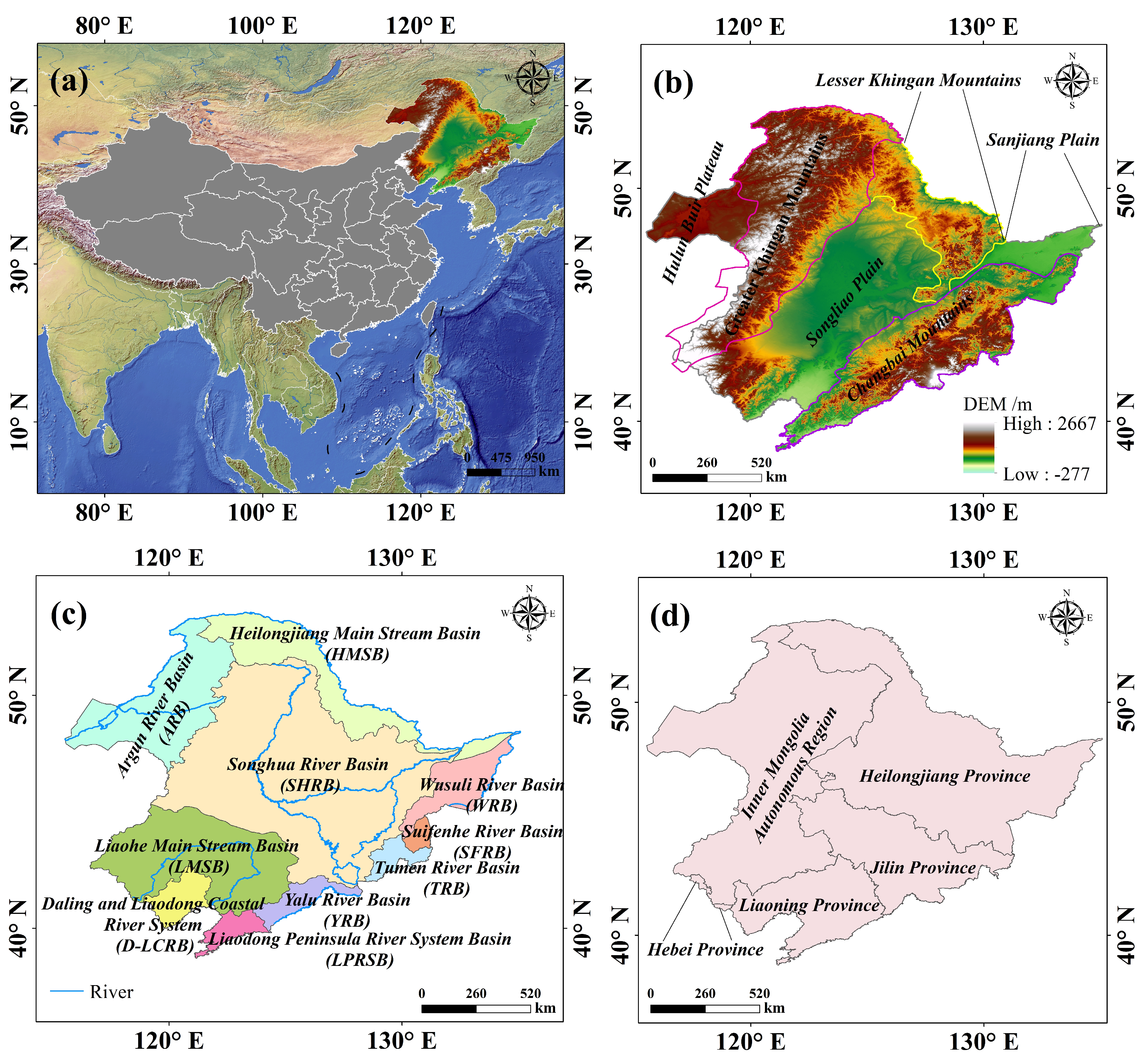
3.1. Description of Songliao River Basin

The Songliao River Basin (SLRB) is located in Northeast China and is one of the seven major river basins. The SLRB is surrounded by mountains on three sides: the Lesser Khingan Mountains in the north, the Greater Khingan Mountains in the west, and the Changbai Mountains in the east, while the southern part is adjacent to the Bohai Sea and the Yellow Sea. The basin contains numerous rivers, including the Heilongjiang River, Argun River, Songhua River, Wusuli River, Suifen River, Tumen River, Liao River, Yalu River, and other rivers flowing into the sea. The basin features diverse landforms such as plains, mountains, and hills, and its climate is mainly temperate continental monsoon, with some regions characterized by a cold temperate climate [62,63]. The geographic features of the SLRB are shown in Figure 1.

3.2. Data

3.2.1. Observation Data

The historical daily precipitation observation data utilized the CN05.1 gridded observational dataset. This dataset utilized observational data from over 2400 meteorological stations across China and established a gridded dataset with a spatial resolution of 0.25° × 0.25° using interpolation methods [64]. The data can be accessed at the Climate Change Research Center (https://ccrc.iap.ac.cn/index.php/resource, accessed on 15 June 2024). Based on the CN05.1 dataset, this paper selected precipitation data for the SLRB as the study area, with the study period spanning from 1971 to 2014. Additionally, the historical daily average temperature data used as influencing factors also originated from the CN05.1 dataset.

3.2.2. Simulation and Prediction Data

This paper used daily precipitation data provided by the Coupled Model Intercomparison Project Phase 6 Global Climate Models (CMIP6 GCMs) for historical simulation evaluation and future prediction of precipitation. The data were accessible through the Earth System Grid Federation (https://esgf-node.llnl.gov/search/cmip6, accessed on 18 June 2024). We selected historical simulation experiment data and future projection experiment data under the Shared Socioeconomic Pathways (SSPs) provided by the Scenario Model Intercomparison Project (ScenarioMIP) from 22 models within CMIP6. For future SSPs projections, the study focused on low (SSP126), medium (SSP245), and high (SSP585) scenarios. The chosen models are listed in

Table 1. The description of selected CMIP6 GCMs.

Model	Institution ID	Country	Resolution (Longitude × Latitude)
ACCESS-CM2	CSIRO	Australia	1.875° × 1.25°
ACCESS-ESM1-5	CSIRO	Australia	1.875° × 1.25°
BCC-CSM2-MR	BCC	China	1.125° × 1.125°
CanESM5	CCCMA	Canada	2.813° × 2.813°
CESM2-WACCM	NCAR	USA	1.25° × 0.938°
CMCC-CM2-SR5	CMCC	Italy	1.25° × 0.938°
CMCC-ESM2	CMCC	Italy	1.25° × 0.938°
EC-Earth3	EC-Earth-Consortium	Europe	0.703° × 0.703°
EC-Earth3-Veg	EC-Earth-Consortium	Europe	0.703° × 0.703°
EC-Earth3-Veg-LR	EC-Earth-Consortium	Europe	1.125° × 1.125°
FGOALS-g3	CAS	China	2° × 2.25°
IITM-ESM	CCCR-IITM	India	1.875° × 1.915°
INM-CM4-8	INM	Russia	2° × 1.5°
INM-CM5-0	INM	Russia	2° × 1.5°
IPSL-CM6A-LR	IPSL	France	2.5° × 1.259°
MIROC6	MIROC	Japan	1.406° × 1.406°
MPI-ESM1-2-HR	MPI-M	Germany	0.938° × 0.938°
MPI-ESM1-2-LR	MPI-M	Germany	1.875° × 1.875°
MRI-ESM2-0	MRI	Japan	1.125° × 1.125°
NorESM2-LM	NCC	Norway	2.5° × 1.875°
NorESM2-MM	NCC	Norway	1.25° × 0.938°
TaiESM1	AS-RCEC	China	1.25° × 0.938°

. The scope of CMIP6 GCMs applications and the historical period are consistent with CN05.1. The future period selected is 2026–2100. To study the changes in precipitation closely across different future periods, the future timeframes are divided into near-term (2026–2050), mid-term (2051–2075), and long-term (2076–2100), relative to the historical base period (1990–2014). Similarly, the daily average temperature data used for simulation and prediction as influencing factors were also provided by CMIP6 GCMs.

3.2.3. Geographical Factors Data

The geographical factors studied in this paper include latitude, longitude, and altitude. The latitude and longitude data were obtained from the grid point data and can be extracted using geographical information processing software. The data for altitude were acquired from the Shuttle Radar Topography Mission (SRTM) at a spatial resolution of 90 m and were available on the Geospatial Data Cloud (https://www.gscloud.cn/, accessed on 5 February 2024). When using altitude as a geographical influencing factor, the resolution must be unified to maintain consistency in the study. Therefore, the altitude data were interpolated to match the resolution of the CN05.1 dataset.

3.3. Methods

3.3.1. CMIP6 GCMs Data Processing

From Table 1, it is known that the selected GCMs have varying resolutions. To ensure the accuracy of the study, we applied bilinear interpolation to adjust the models to match the observational data, interpolating to a resolution of 0.25°. Bilinear interpolation [65] is an algorithm used for two-dimensional data interpolation, commonly applied in fields such as image processing and geographic information systems. The interpolated data provided a more detailed representation, enhancing its practicality and usability. Using geographic information processing software for mask extraction, the study area covered the SLRB, comprising a total of 2278 grid points.

3.3.2. Comprehensive Evaluation of CMIP6 GCMs

The paper evaluates how effectively various models can simulate precipitation within the SLRB from multiple aspects, including mean precipitation, spatiotemporal characteristics, and variation trends. The specific evaluation metrics are shown in

Table 2. The description of evaluation indicators.

Evaluation Feature	Specific Indicator
Mean	Mean annual precipitation (mean)
Time feature	Inter-annual variability skill (IVS)
	Pearson correlation coefficient for intra-annual monthly precipitation (CCt)
Trend variation	Significance statistic of Mann–Kendall trend test (Z)
	Slope statistic of Mann–Kendall trend test (slope)
Spatial feature	Pearson correlation coefficient for spatial characteristics (CCs)
	Normalized root-mean-square error (NRMSE)
	Taylor skill score Ⅰ (TSS1)
	Taylor skill score Ⅱ (TSS2)

. Based on nine indicators, an improved ranking score method was used for comprehensive evaluation, making the results more intuitive. The improved ranking score method [66] distinguishes between relative error indicators and non-relative error indicators, effectively differentiating indicators with different evaluation scales and calculating them separately. Each model’s score for each indicator ranges from 0 to 1, with higher scores indicating better simulation. The calculation is as follows:

$$R{S}_i=\left\{\begin{array}{c} {\displaystyle \frac{T_i-T_{min}}{T_{max}-T_{min}}}, T is non-relative error indicator\\ 1-{\displaystyle \frac{T_i-T_{min}}{T_{max}-T_{min}}}, T is relative error indicator\end{array}\right.$$

(1)

In the formula, RS_i represents the score of the i-th model, Ti is the calculated value of the evaluation indicator for the i-th model, and T_max and T_min are the corresponding maximum and minimum values. To more intuitively quantify the differences between simulated means (mean), trend variations (Z-value and slope), and real values, absolute errors are used in evaluation. The non-relative error indicators include CC_t, CC_s, TSS₁, and TSS₂ [67]; the closer these indicators are to 1, the better the simulation performance. The relative error indicators include mean, IVS [68], NRMSE [69], Z-value, and slope [70]; the closer these indicators are to 0, the better the simulation performance. For cases with two evaluation indicators representing the same descriptive method, such as Z and slope in trend analysis, as well as TSS₁ and TSS₂ in Taylor evaluation metrics, a weight of 0.5 is assigned to each. Other evaluation indicators are assigned a weight of 1.

3.3.3. Weighted Multi-Model Ensemble Average

Based on the improved ranking score method, different weights were calculated according to the comprehensive scores, and these weights were assigned to the respective models to obtain the multi-model ensemble data. The calculation is as follows:

$$W_i={\displaystyle \frac{R{S}_i}{{{\displaystyle \sum }}_{i=1}^{n}R{S}_i}}$$

(2)

$$P_{MM{E}_n}={{\displaystyle \sum }}_{i=1}^n{W}_i\times P_i$$

(3)

In the formula, RS_i is the score of the i-th model, W_i is the weight of the i-th model, P_i is the precipitation amount from the i-th model, and P_MMEn is the precipitation amount after the multi-model ensemble.

3.3.4. Bias Correction

To improve the accuracy of the simulation, the Delta downscaling method was used to bias-correct the precipitation (temperature) data derived from the multi-model ensemble mean. The Delta downscaling method involves obtaining a change factor by comparing the differences between historical model data and observational data, assuming that this change factor remains constant in the future to adjust future model data. This method is widely used, and studies have shown that it performs well in bias correction. The calculation is as follows:

$$P_{cor}=\overline{P_{obs,res}}\times {\displaystyle \frac{P_{gcm}}{\overline{P_{gcm,res}}}}$$

(4)

$$T_{cor}=\overline{T_{obs,res}}+(T_{gcm}-\overline{T_{gcm,res})}$$

(5)

In the formula, $\overline{P_{obs,res}}$ ($\overline{T_{obs,res}}$) is the long-term average precipitation (temperature) from observational data over the reference period, $\overline{P_{gcm,res}}$ ($\overline{T_{gcm,res}}$) is the long-term average precipitation (temperature) simulated by the models over the reference period, P_gcm (T_gcm) is the precipitation (temperature) series simulated by the models for the validation or future period, and P_cor (T_cor) is the bias-corrected precipitation (temperature) series. The reference period is 1971–2000, the validation period is 2001–2014, and the future period is 2026–2100.

3.3.5. Characteristic Analysis of Precipitation

Linear trend analysis [71] is a statistical method used to identify and quantify trends in data over time, describing the relationship between variables through the use of linear regression models. It can effectively identify and quantify the temporal changes in precipitation data, providing a clear trend line to aid in understanding long-term variations in precipitation. The cumulative anomaly method [72] can be used to analyze the changes in meteorological elements relative to long-term averages by calculating the deviation (anomaly) between observed values and long-term averages and accumulating these deviations. This study employed linear trend analysis and cumulative anomaly methods to investigate the historical precipitation processes in the SLRB. Similarly, the trends of future precipitation change under different scenarios were analyzed to identify the temporal evolution patterns of precipitation. By comparing historical precipitation with future projections, the spatiotemporal variations in future precipitation (near-term, mid-term, and long-term) were demonstrated. Using geographic information processing software, the spatial patterns and trend analyses of historical and future annual precipitation were visualized, with isohyets drawn to illustrate changes in dry and wet patterns. This provided a better understanding of the spatial variations in precipitation. Pearson correlation analysis [73] is a statistical method used to measure the strength and direction of the linear relationship between two continuous variables. It was applied to explore the influence of geographic factors (latitude, longitude, and altitude) on precipitation, revealing how precipitation varies with geographic indicators. Besides, a linear regression function was established between the changes in future precipitation relative to the historical baseline and the changes in future mean temperature relative to the historical baseline, with the slope representing the response rate, to quantify the impact of temperature change on precipitation within the SLRB [74].

4. Results

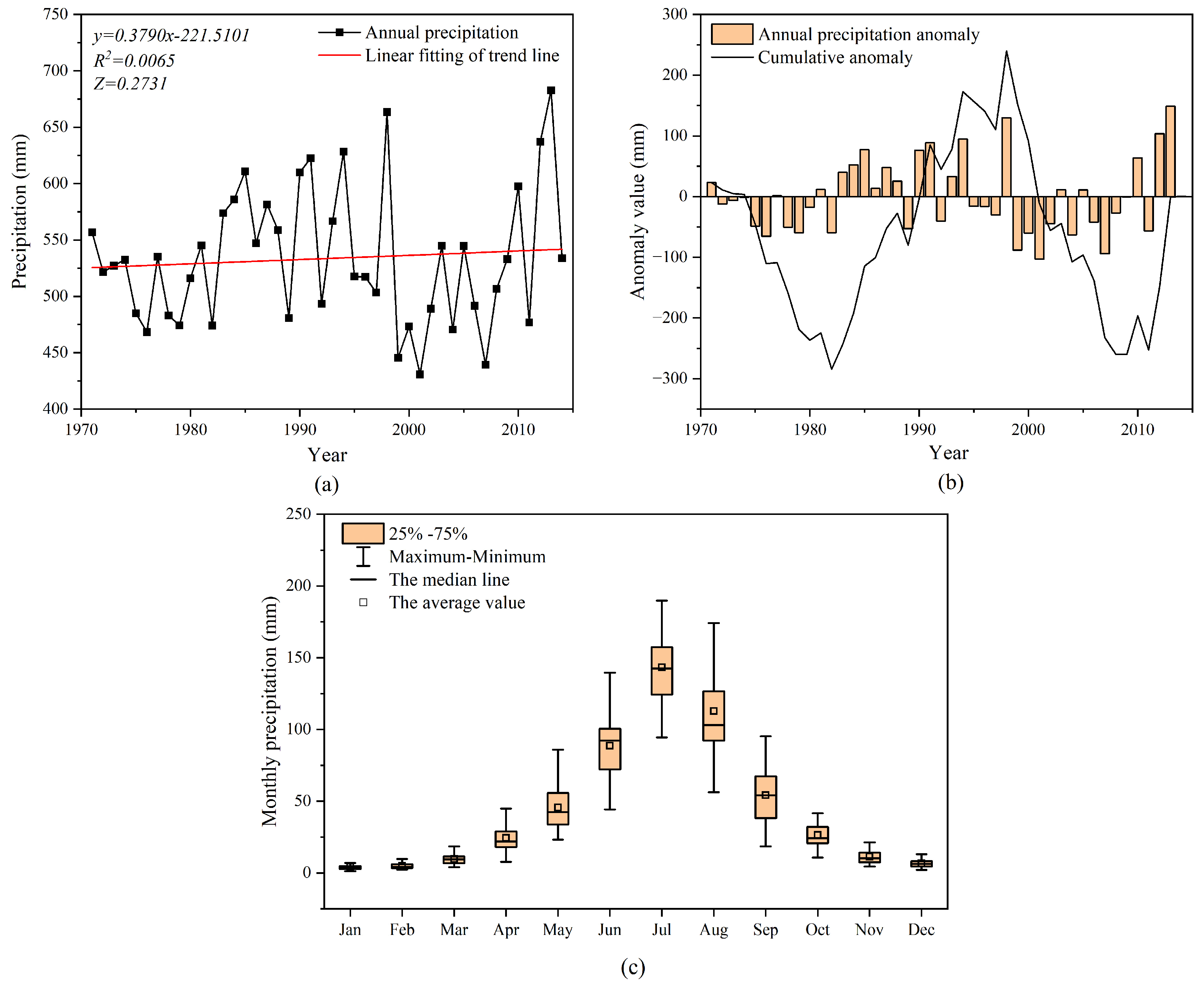
4.1. Climatological Characteristics of Observed Precipitation

Figure 2 analyzed the temporal variation in precipitation from annual and monthly perspectives for 1971–2014. The Mann–Kendall test yielded a Z-value of 0.2731, indicating that the overall precipitation exhibited a non-significant increasing trend. Similarly, the results of linear trend fitting also reflected this trend, with a precipitation tendency rate of 3.79 mm/10a (Figure 2a). From the cumulative anomaly curve in Figure 2b, it can be observed that the curve generally shows a “W” shape, indicating that the annual precipitation changes in the basin during 1971–2014 can be divided into four stages: “decrease (1971–1982)—increase (1983–1998)—decrease (1999–2009)—increase (2010–2014)”. Abrupt changes were identified in 1982, 1998, and 2009. The monthly precipitation distribution exhibited distinct characteristics, with precipitation increasing from January to a peak and then decreasing toward December (Figure 2c). Precipitation was mainly concentrated between May and September, with a specific amount of 444.97 mm, accounting for 83.4% of the total annual precipitation. July experienced the highest precipitation, with an average monthly precipitation of 143.37 mm. In contrast, January, February, and December had very low precipitation, with average monthly precipitation below 10 mm.

Figure 3 analyzes the spatial characteristics of precipitation in the SLRB from 1971 to 2014 in terms of distribution patterns and trend changes. The annual precipitation showed an overall increasing pattern from northwest to southeast (Figure 3a). Based on the isohyets, the multi-year average precipitation in the southeastern region exceeded 800 mm, classifying it as a humid area, with a maximum of 1071.41 mm. In contrast, the multi-year average precipitation in the northwestern region was generally below 400 mm, making it a semiarid area, with a minimum of 261.82 mm. Additionally, some areas in the southwestern part of the SLRB also received less than 400 mm of precipitation, similarly classified as semiarid zones. From 1971 to 2014, most areas exhibited an increasing precipitation trend. Notably, the southeastern part of the SHRB (sub-basin) showed a significant upward trend (p < 0.05), with a change rate ranging from 31.11 mm/10a to 47.43 mm/10a. In contrast, areas with decreasing precipitation trends were mainly concentrated in the southwestern part of the SLRB, where the largest decrease reached 13.17 mm per decade (Figure 3b).

4.2. Evaluation of CMIP6 GCMs on the Precipitation in the Songliao River Basin

4.2.1. Evaluation Based on Spatiotemporal Characteristics

From the temporal scale perspective, the evaluation indicators mainly included annual precipitation mean, inter-annual variability, changes in monthly precipitation within the year, and trends over time. The statistical values of these indicators are shown in

Table 3. Evaluate the statistics of spatiotemporal scale indicators.

Model	Temporal Scale					Spatial Scale
	Mean	IVS	CCt	Z	Slope	CCs	NRMSE	TSS1	TSS2
CN05.1	533.578	/	/	0.273	0.226	/	/	/	/
ACCESS-CM2	575.855	0.236	0.963	0.860	0.875	0.826	0.112	0.911	0.694
ACCESS-ESM1-5	692.944	0.301	0.981	−1.325	−1.218	0.664	0.251	0.832	0.480
BCC-CSM2-MR	532.972	0.189	0.977	0.435	0.260	0.873	0.083	0.875	0.720
CanESM5	604.875	0.324	0.987	0.010	0.026	0.603	0.193	0.773	0.399
CESM2-WACCM	690.223	0.701	0.993	1.446	1.609	0.839	0.239	0.862	0.671
CMCC-CM2-SR5	793.744	0.602	0.991	1.487	1.507	0.735	0.365	0.868	0.567
CMCC-ESM2	755.731	0.379	0.989	1.972	1.540	0.723	0.319	0.861	0.551
EC-Earth3	610.007	0.182	0.989	2.761	2.411	0.921	0.132	0.918	0.815
EC-Earth3-Veg	632.757	0.145	0.990	0.273	0.335	0.922	0.155	0.922	0.820
EC-Earth3-Veg-LR	599.069	0.102	0.976	0.779	0.601	0.919	0.124	0.905	0.801
FGOALS-g3	487.303	0.534	0.992	1.709	1.091	0.605	0.179	0.773	0.400
IITM-ESM	689.578	0.153	0.946	0.920	0.730	0.81	0.230	0.902	0.670
INM-CM4-8	828.867	0.318	0.988	1.406	1.464	0.716	0.421	0.793	0.502
INM-CM5-0	838.705	0.420	0.987	−1.163	−1.045	0.757	0.421	0.877	0.595
IPSL-CM6A-LR	729.119	0.279	0.976	1.507	1.367	0.816	0.302	0.759	0.569
MIROC6	748.081	0.338	0.974	2.640	2.313	0.729	0.326	0.773	0.500
MPI-ESM1-2-HR	699.741	0.236	0.943	−0.192	−0.149	0.841	0.244	0.897	0.701
MPI-ESM1-2-LR	782.851	0.208	0.934	−0.981	−0.926	0.886	0.339	0.943	0.792
MRI-ESM2-0	641.934	0.285	0.987	−0.152	−0.232	0.794	0.176	0.861	0.623
NorESM2-LM	609.174	0.256	0.989	0.111	0.108	0.874	0.131	0.864	0.711
NorESM2-MM	604.195	0.313	0.993	1.790	1.437	0.872	0.125	0.930	0.764
TaiESM1	747.344	0.203	0.977	−0.678	−0.636	0.844	0.300	0.915	0.718

The bolded statistics simulated the top five models that work best for this indicator.

. Considering the mean, the annual mean precipitation in the SLRB from 1971 to 2014 was 533.578 mm. The simulation range of the CMIP6 GCMs was 487.303 to 838.705 mm. Except for the FGOALS-g3 and BCC-CSM2-MR, the other models overestimated precipitation in the basin. Among the many models, BCC-CSM2-MR had the annual average precipitation closest to the observed data, at 532.972 mm, with a deviation of only −0.606 mm, indicating the best simulation performance. It was followed by ACCESS-CM2, FGOALS-g3, EC-Earth3-Veg-LR, NorESM2-MM, CanESM5, NorESM2-LM, EC-Earth3, and EC-Earth3-Veg, all with deviations within 100 mm. The INM-CM5-0 model performed the worst, with a simulated annual average precipitation of 838.705 mm, overestimating it by more than 300 mm.

Regarding the inter-annual variability, the range of the simulated index was 0.102 to 0.701. The IVS being closer to 0 indicates a superior simulation of inter-annual variability [75]. All selected models had IVS values less than 1, indicating that the CMIP6 GCMs can reasonably replicate the inter-annual variations in the SLRB. Among them, the EC-Earth3-Veg-LR, EC-Earth3-Veg, IITM-ESM, EC-Earth3, and BCC-CSM2-MR models exhibited the best performance in simulation. The analysis of the simulation effect on intra-annual variation focused primarily on the assessment of monthly precipitation scales. The Pearson correlation coefficient (CC_t) showed the correlation between true values and simulated values of monthly average precipitation, with results being quite good as all values exceed 0.9. Compared to other models, CESM2-WACCM and NorESM2-MM had the highest CC_t value of 0.993, making them the two models with the best simulation performance for this evaluation indicator.

From the perspective of precipitation trend changes, precipitation within the SLRB showed an insignificant upward trend from 1971 to 2014 (Z < 1.96), with a change rate of 0.226 mm/a. Regarding the trend changes simulated by the models, most models were able to simulate the upward trend in precipitation during this period, with only six models showing a downward trend: ACCESS-ESM1-5, INM-CM5-0, MPI-ESM1-2-HR, MPI-ESM1-2-LR, MRI-ESM2-0, and TaiESM1. The BCC-CSM2-MR, EC-Earth3-Veg, and NorESM2-LM not only demonstrated the upward trend but also had a slope close to the observed real slope, with deviations within ±0.1 mm/a, demonstrating significant simulation advantages.

From the spatial scale perspective, the evaluation metrics mainly included the correlation coefficient for spatial precipitation (CC_s), normalized root-mean-square error (NRMSE), and Taylor skill scores (TSS₁ and TSS₂), with the statistical values shown in Table 3. The range of CC_s was 0.603~0.922, indicating that most models performed well in simulating the spatial distribution of multi-year precipitation in the SLRB. Among these models, EC-Earth3, EC-Earth3-Veg, and EC-Earth3-Veg-LR had the highest CC_s, demonstrating the best performance in simulating spatial distribution patterns. The range of NRMSE was concentrated between 0.083 and 0.421. The relatively small NRMSE values across all models indicated that the CMIP6 models performed well in simulating precipitation. Among them, BCC-CSM2-MR, ACCESS-CM2, EC-Earth3-Veg-LR, NorESM2-MM, and NorESM2-LM demonstrated the best simulation performance. The TSS₁ and TSS₂ ranged from 0.759 to 0.943 and 0.399 to 0.820, respectively. Although there were differences in TSS values among the models, considering both skill scores comprehensively, the models with better performance in simulating spatial patterns were consistent. These models included EC-Earth3, EC-Earth3-Veg, MPI-ESM1-2-LR, and NorESM2-MM.

To provide a more detailed depiction of how different models simulate spatial precipitation, the relative error of the model simulations was visualized, as presented in Figure 4. There was significant spatial heterogeneity in the deviations between different models and observed precipitation. Many models exhibited a wet bias when simulating spatial precipitation. This was particularly evident in CMCC-CM2-SR5, CMCC-ESM2, INM-CM4-8, INM-CM5-0, and MIROC6, where areas like the WRB, the SFRB, the TRB (in the northeast of the SLRB), the ARB (in the northwest of the SLRB), and the western LMSB (in the southwest of the SLRB) showed wet biases exceeding 90% and reaching up to 153%. In contrast, FGOALS-g3 mostly showed a dry bias in simulating annual precipitation, except for displaying a wet bias in areas such as the SFRB, the TRB, and the Greater Khingan Mountains. ACCESS-CM2, BCC-CSM2-MR, EC-Earth3, EC-Earth3-Veg, EC-Earth3-Veg-LR, MRI-ESM2-0, NorESM2-LM, and NorESM2-MM performed better in simulating the spatial distribution patterns of annual precipitation within the SLRB, with deviations controlled within −20% to 50%, and no instances of overly dry or wet conditions within the basin. Overall, the CMIP6 GCMs tended to significantly overestimate precipitation in the northeastern, southwestern, and northwestern parts of the SLRB, while wet bias weakened in the southeastern part, where some models instead exhibited a dry bias.

4.2.2. Comprehensive Evaluation and Multi-Model Ensemble Average

By comparing evaluation metrics across temporal and spatial scales, differences in the performance of the models were observed. To determine the models best suited for simulating precipitation in the SLRB, a comprehensive score was calculated for all indicators. Figure 5a presents the comprehensive scores of all models for precipitation simulation. It can be seen that EC-Earth3-Veg performs the best in simulating precipitation, followed by BCC-CSM2-MR, EC-Earth3-Veg-LR, NorESM2-LM, NorESM2-MM, EC-Earth3, ACCESS-CM2, MRI-ESM2-0, TaiESM1, and IITM-ESM. These models all scored above the median score of 4.07, which basically satisfied the spatiotemporal characteristics of precipitation in the basin during the observation period.

A single model may be affected by its specific biases and limitations, while a multi-model ensemble can reduce these uncertainties by integrating outputs from different models, thereby capturing the potential uncertainties of climate change more comprehensively. Using an improved ranking score method, composite scores were calculated, and based on the ranking of these scores, weights were assigned to create a multi-model ensemble dataset. MME1 represents the single climate model with the best predictive performance (EC-Earth3-Veg), and so on, up to MME22, which represents the weighted average of all climate models in the ensemble. Figure 5b shows the ranking scores for the effectiveness of precipitation simulations by the multi-model ensemble data. The results in the figure indicated that the simulation performance of MME2 to MME9 was superior to MME1, with MME2 performing the best, achieving a composite score of 6.15, followed by MME4 with a score of 6.07. As weaker models were included, the performance of precipitation simulation became progressively worse. This indicated that selecting certain optimal models to form a multi-model ensemble (MME) for precipitation simulation in the SLRB would yield better results. Therefore, we preliminarily chose MME2, consisting of EC-Earth3-Veg and BCC-CSM2-MR, as the dataset to simulate future precipitation. The weights assigned to the two models were 0.507 and 0.493, respectively.

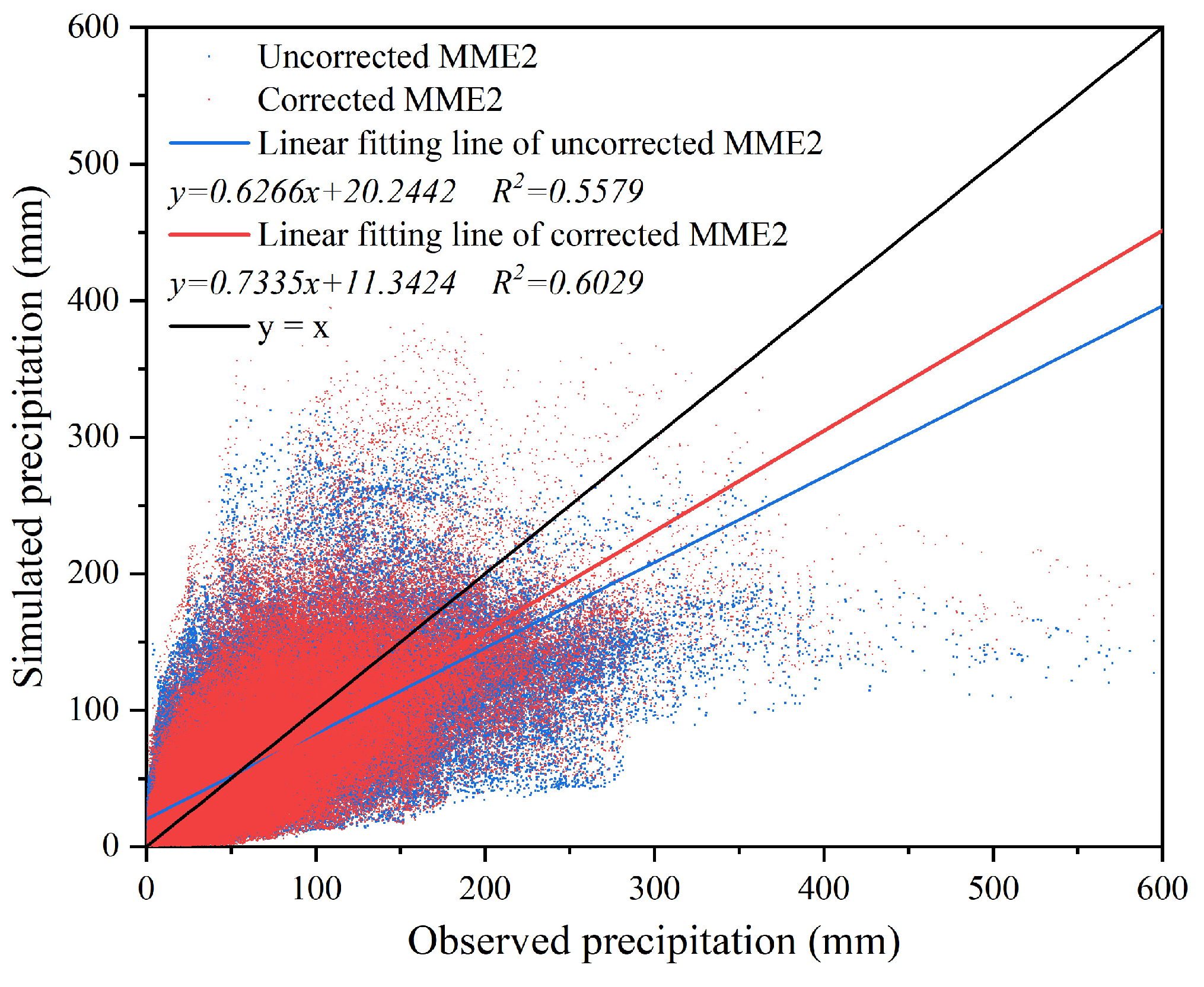
4.2.3. Bias Correction for MME2

To further improve the accuracy of predictions, the Delta downscaling method was applied to MME2 for bias correction. The precipitation data from 1971–2000 were used as the training period to derive correction factors, and 2001–2014 were used as the validation period to assess the effectiveness of the correction. Figure 6 illustrates the changes in performance before and after bias correction during the validation period. As shown in Figure 6, the fit (R²) between the uncorrected MME2 dataset and the observed data was 0.5579, while the corrected data achieved an improved R² of 0.6029. Additionally, the linear regression line after correction was closer to the y = x line, indicating better alignment with the observations.

Figure 7 shows the spatial distribution of annual precipitation bias before and after correction. Before correction, the spatial bias of MME2-simulated precipitation ranged from −16% to 37%, but after correction, this bias was reduced to −11% to 18%. The areas with a significant overestimation of precipitation were effectively alleviated. Additionally, the spatial correlation coefficients of precipitation before and after correction were calculated. The spatial correlation coefficient for the uncorrected MME2 precipitation data during the validation period was 0.918, which improved to 0.979 after bias correction. This indicated that the bias-corrected data can enhance the accuracy of spatial predictions and increase the reliability of the data. Therefore, we used the bias-corrected MME2 data to study future precipitation changes in the SLRB.

4.3. Future Prediction of Precipitation in Songliao River Basin from 2026 to 2100

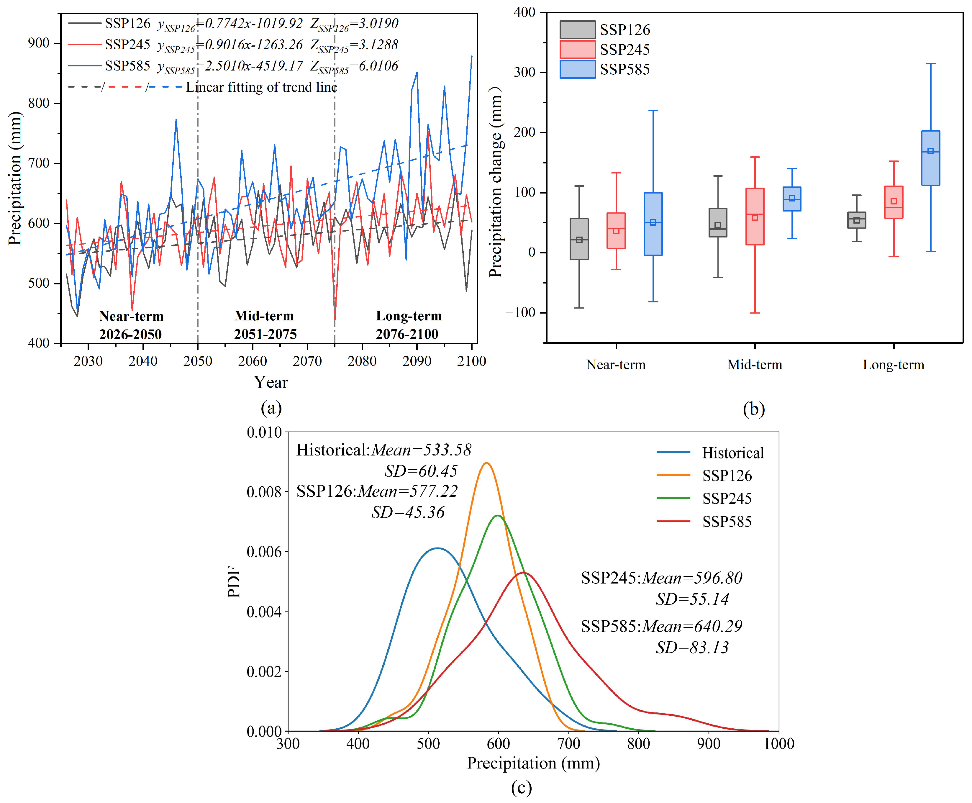
4.3.1. Temporal Evolution of Precipitation

Over time, the evolution of future precipitation in the SLRB was analyzed. Under low-, medium-, and high-emission scenarios, the future precipitation showed a significant upward trend (p < 0.01). The rates of change in basin-wide precipitation during 2026–2100 were 7.742 mm/10a (SSP126), 9.016 mm/10a (SSP245), and 25.01 mm/10a (SSP585) (Figure 8a). It is evident that under the high-emission scenario, future precipitation will increase more dramatically. Figure 8b shows the changes in precipitation under SSPs relative to the base period across different time periods. From the near term to the medium term and then the long term, the magnitude of precipitation increase grows in all scenarios, with the long-term precipitation increase under SSP585 being the most significant. Under SSP126, precipitation changes in the long term are more concentrated compared to the near term and medium term, indicating that precipitation changes under the low-emission scenario remain stable in the long term, showing a relatively steady precipitation pattern. Under SSP245, the box plot for mid-term precipitation is more dispersed compared to near-term and long-term precipitation, indicating greater variability in precipitation during 2051–2075. In contrast to SSP245, under SSP585, mid-term precipitation is more stable, while precipitation variability is greater in the near term and long term. Figure 8c illustrates the probability distribution of precipitation under historical precipitation and SSPs. From the historical period to the future, the probability density curves of annual average precipitation gradually shift to the right, indicating an increase in total precipitation. From the low-emission to high-emission scenario, the probability density curves become flatter, and the standard deviation increases, indicating that precipitation variability will intensify under the high-emission scenario.

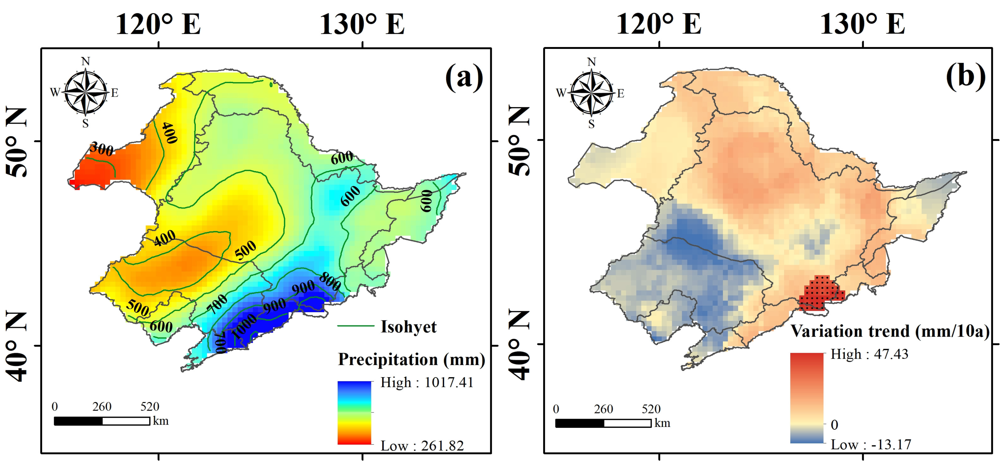
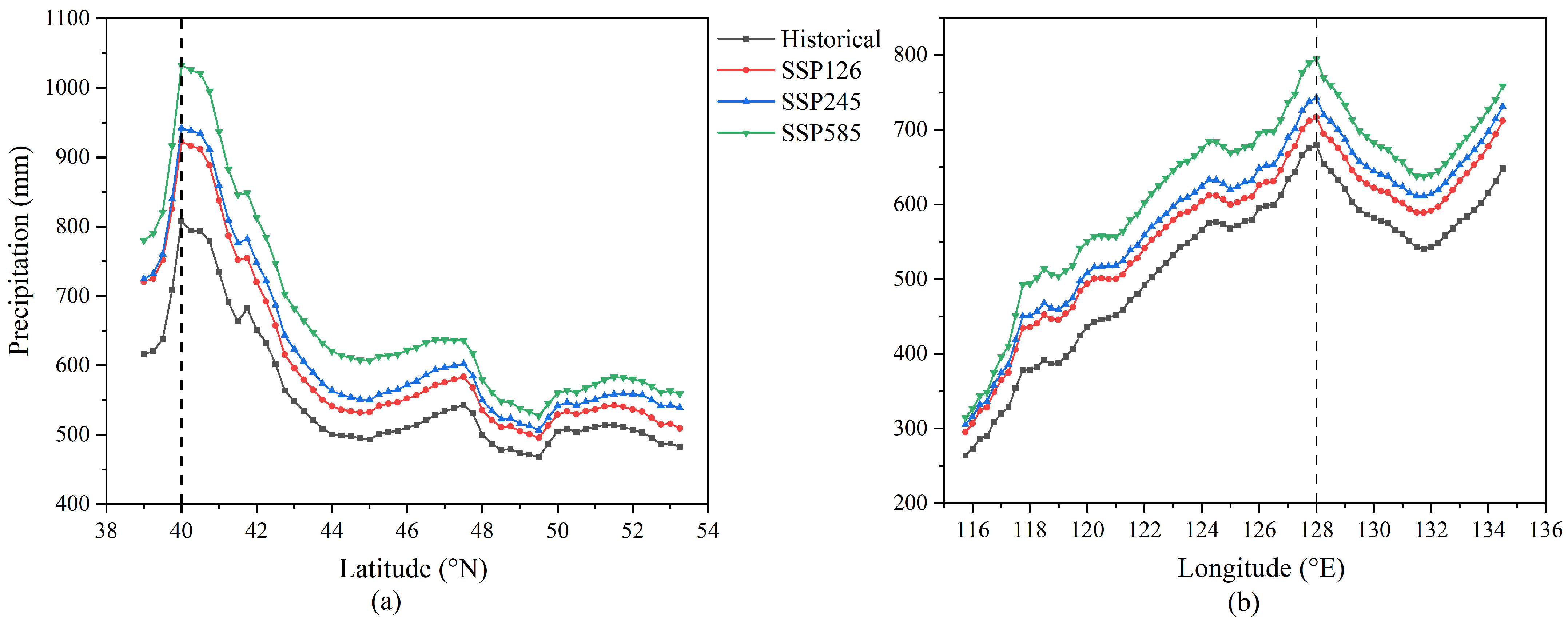
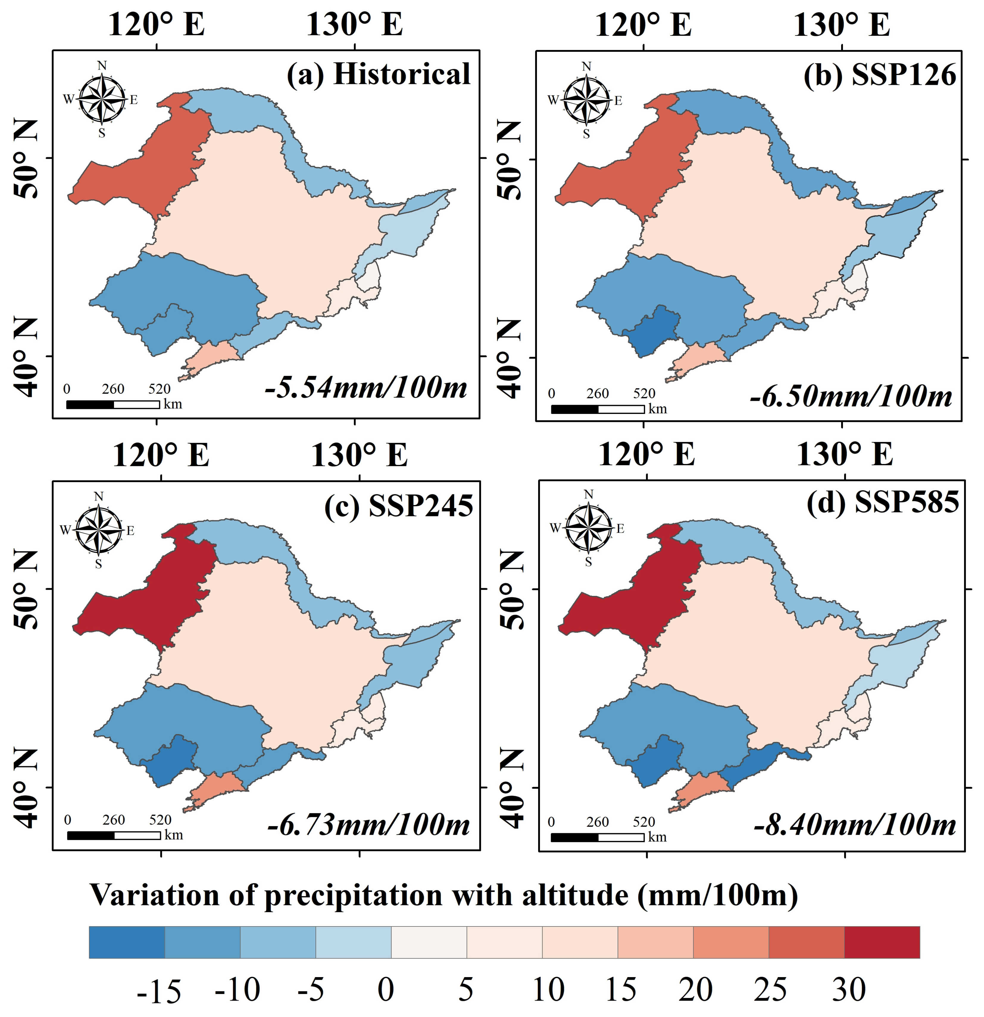
4.3.2. Spatial Change Pattern of Precipitation

Figure 9 shows the spatial pattern and trend distribution for precipitation within the SLRB from 2026 to 2100. In various scenarios, the spatial pattern of precipitation continued to increase from northwest to southeast, and the distribution of isohyets was basically the same (Figure 9a–c). Compared with historical precipitation, future isohyets gradually shift northwestward, with the semiarid area shrinking and the humid area expanding, a phenomenon more evident under the high-emission scenario (Figure 9d). From 2026 to 2100, under SSP126, precipitation showed an increasing trend across the entire basin, with a significant rise in the eastern part of the basin. The overall change rate ranged from 0.82 mm/10a to 30.09 mm/10a, with areas experiencing the most significant increase concentrated in the southeastern part of the SLRB (the YRB and the LPRSB), where the trend change rate exceeded 20 mm/10a. Under SSP245, the precipitation trend showed a slight decrease in the northeastern part of the basin, while the rest of the region exhibited an increasing trend. Significant increases were observed in the northeastern and southwestern parts of the basin, with the overall change rate ranging from −0.60 mm/10a to 26.26 mm/10a. The areas with the largest increase were concentrated in the southern part of the basin. Under SSP585, the entire basin showed a significant increasing trend, with a change rate ranging from 8.46 mm/10a to 59.79 mm/10a. Compared to the other two scenarios, the upward trend was more pronounced. The increasing trend in precipitation decreased from south to north, with the southern part of the SLRB showing a trend change rate exceeding 30 mm/10a. As the climate warms, both the total annual precipitation and precipitation trends show an increasing pattern. Particularly under SSP585, the findings suggest a potential for higher flood risks in the future, with more severe increases in precipitation and extreme rainfall events likely to occur.

Figure 10 presents the spatial precipitation change rates in the SLRB under future scenarios across different periods relative to the base period. Under SSP126, most areas exhibited an increasing trend compared to the base period across all time periods, with only slight decreases (within −10%) in certain parts of the basin. Compared to the near-term period, the mid-term and long-term periods showed greater increases, with a particularly significant increase in the southwestern part. Under SSP245, in the near and medium terms, some areas of the SHRB (sub-basin) still showed a decreasing trend, but the magnitude of the decrease further weakened (within −4%), while the rest of the region exhibited increases ranging from 0% to 28%. In the long term, the entire basin showed a consistent increasing trend, with the magnitude of the increase becoming even greater. The southwestern part of the SLRB experienced the largest increase, ranging from 20% to 40%. Compared to SSP126 and SSP245, the SSP585 showed a larger magnitude of increase, with a greater extent of high-value areas. In the near term, some areas of the SHRB (sub-basin) still showed a decreasing trend (within −3%), but the area of decrease became smaller. Compared to the near and medium terms, the long-term growth was significantly larger, with a noticeable increase in high-value areas. In particular, the southwestern part of the SLRB showed an increase exceeding 40%.

4.4. Factors Influencing Precipitation in the Songliao River Basin

4.4.1. Geographical Factors

Using the Pearson correlation analysis method, the study investigated the influence of geographical factors (latitude, longitude, and altitude) on precipitation in the SLRB. The results are shown in

Table 4. Correlation coefficients between precipitation and latitude, longitude, and altitude.

	Latitude	Longitude	Altitude
Precipitation—historical	−0.746 a	0.838 a	−0.136 a
Precipitation—SSP126	−0.780 a	0.854 a	−0.150 a
Precipitation—SSP245	−0.777 a	0.853 a	−0.150 a
Precipitation—SSP585	−0.819 a	0.811 a	−0.173 a

“^a” stands for passing the 0.01 significance level criterion.

. Precipitation in the basin is closely related to geographical factors. Specifically, latitude had a significant negative correlation with precipitation (p < 0.01), with a correlation coefficient of −0.746 during the historical period, and −0.780 (SSP126), −0.777 (SSP245), and −0.819 (SSP585) under different future scenarios. Longitude, on the other hand, had a significant positive correlation with precipitation (p < 0.01), with a correlation coefficient of 0.838 during the historical period and 0.854 (SSP126), 0.853 (SSP245), and 0.811 (SSP585) under different future scenarios. The correlation analysis results indicated that areas with lower latitudes and higher longitudes tended to experience more precipitation. Figure 11 further analyzes how precipitation varies with latitude and longitude. From the perspective of latitude, the curve exhibits a major peak around 40° N, after which precipitation variability decreases as latitude increases. From the perspective of longitude, the curve also displays a peak near 128°E, followed by a small trough. Regardless of whether it is the historical period or various future scenarios, the curves exhibit similar variation patterns, with precipitation gradually increasing over time.

According to Table 4, comparatively, the correlation coefficient between altitude and precipitation is smaller. During the historical precipitation period, the correlation coefficient was −0.136, while during the future precipitation period, the correlation coefficients under different scenarios were −0.150 (SSP126), −0.150 (SSP245), and −0.173 (SSP585), indicating a significant negative correlation. This suggests that areas at lower altitudes are likely to receive more precipitation. Figure 12 shows the variation in precipitation with altitude in the SLRB and its sub-basins. From historical to future periods, the variation in precipitation with altitude in the entire basin is −5.54 mm/100 m (historical), −6.50 mm/100 m (SSP126), −6.73 mm/100 m (SSP245), and −8.40 mm/100 m (SSP585). However, for sub-basins, the precipitation in some sub-basins increases with altitude (ARB, SHRB, SFRB, TRB, LPRSB), among which ARB and LPRSB exhibit the most significant increases, with expected increases of 32.20 mm/100 m and 23.52 mm/100 m under SSP585. In contrast, the precipitation in other sub-basins decreases with altitude (HMSB, WRB, LMSB, D-LCRB, YRB), with D-LCRB and YRB showing the most notable decreases, with expected reductions of −18.91 mm/100 m and −17.14 mm/100 m under SSP585.

4.4.2. Temperature Rise Factors

Using the MME2, composed of EC-Earth3-Veg and BCC-CSM2-MR, and applying Delta bias correction, the future temperature changes within the SLRB were analyzed. The multi-year average temperature during the historical baseline period was 2.65 °C. From 2026 to 2100, under low-, medium-, and high-emission scenarios, the future multi-year average temperatures are projected to be 4.31 °C, 5.06 °C, and 6.72 °C, respectively. This indicates a significant warming trend in the SLRB in the future. Figure 13 illustrates the relative changes in mean temperature compared to the base period. From 2026 to 2100, the mean temperature in the basin showed an increasing trend, with rates of change of 0.124 °C/10a (SSP126), 0.360 °C/10a (SSP245), and 0.832 °C/10a (SSP585) (Figure 13a). Spatially, under the low-, medium-, and high-emission scenarios, the temperature was projected to increase by 1.66 °C, 2.43 °C, and 4.10 °C, respectively, relative to the base period. Additionally, the northern part of the basin was expected to experience a greater temperature increase compared to the southern part (Figure 13A–C). The temperature differences within the basin were 0.64 °C, 0.89 °C, and 1.41 °C for SSP126, SSP245, and SSP585, respectively. Combining Figure 8a and Figure 13a, it can be observed that both precipitation and temperature in the SLRB show an upward trend in the future. However, the response relationship between future precipitation and temperature needs further investigation.

Figure 14 quantifies the response of future precipitation in the SLRB to temperature changes. Under SSP126, precipitation exhibited a negative response, meaning that precipitation decreases as temperature rises, with a response rate of −0.95%/°C. However, under SSP245 and SSP585, precipitation showed a positive response to temperature, with the response being more sensitive under SSP585, at response rates of 2.40%/°C and 4.87%/°C, respectively (Figure 14a). At the sub-basin level (Figure 14b), D-LCRB, LMSB, and LPRSB showed higher response rates of precipitation to temperature changes. As temperature increases, precipitation growth in these sub-basins became more pronounced, with an average response rate exceeding 8%/°C across scenarios. Compared to SSP126 and SSP245, the response rates under SSP585 were more concentrated across the sub-basins. Notably, in some sub-basins, the response rates under the low-emission scenario were significantly higher than those under the high-emission scenario, such as ARB, D-LCRB, LPRSB, and WRB. This may be attributed to the fact that under the high-emission scenario, the mean temperature increase is disproportionately large relative to precipitation changes.

5. Discussion

5.1. Analysis of CMIP6 GCMs’ Simulation Effect

This study utilized 22 global climate models from CMIP6 to simulate the spatiotemporal variation for precipitation within the SLRB and selected some of the well-performing models’ output data for forecasting. The research conducted a comprehensive assessment based on mean precipitation, spatiotemporal characteristics, and variation trends, using an improved ranking score method. The results indicated that models such as EC-Earth3-Veg, BCC-CSM2-MR, EC-Earth3-Veg-LR, NorESM2-LM, and NorESM2-MM exhibited superior performance in simulating precipitation. It was noteworthy that, aside from NorESM2-LM, the other well-performing models among those selected generally had higher resolutions. For instance, the original resolution of EC-Earth3 and EC-Earth3-Veg can reach 0.703° × 0.703°. In contrast, models with lower resolutions, such as INM-CM4-8, tended to perform poorly in precipitation simulations. Generally, high-resolution models are capable of effectively capturing regional-scale precipitation phenomena, whereas low-resolution models may miss some critical precipitation mechanisms [76]. However, model resolution is not the sole criterion for evaluating simulation performance. For example, although the original resolution of NorESM2-LM is 2.5° × 1.875°, it was still able to effectively capture the precipitation characteristics of the basin. This indicates that the model’s structure, physical processes, initial states of the ocean and land surfaces, as well as biases in boundary conditions are also important factors that cannot be overlooked. In the process of simulating precipitation in the SLRB, most models tended to overestimate actual precipitation amounts. Historical studies have pointed out that one reason for this overestimation was that global climate models often simulate more convective precipitation [77].

Although this study has identified some well-performing models for reproducing precipitation characteristics in the basin, the results from individual models still exhibit significant uncertainty. To reduce uncertainty and bias, a weighted multi-model ensemble average and bias correction were used to further enhance the accuracy of simulated precipitation. The results indicated that the MME2 model output, which included participation from EC-Earth3-Veg and BCC-CSM2-MR, represented the optimal model ensemble. Compared to the multi-model ensemble that included all models, selecting an ensemble of preferred models can avoid the negative impact of less effective models, resulting in more reliable final simulation outcomes. Yang et al. [78] used CMIP6 data to simulate annual precipitation in China and found that selecting well-performing models for the ensemble yielded better results than using the full model ensemble. It is noteworthy that while there are numerous studies utilizing the output data of optimal model ensembles to predict precipitation, there is variability in determining the number of models participating in the optimal ensemble [50,79,80]. Therefore, it is important to emphasize that the number of models in the ensemble should not be a fixed value. Instead, it should be determined through actual research and analysis. The ultimate goal is to identify the optimal ensemble that can best replicate the actual precipitation characteristics to the greatest extent possible. Furthermore, applying the Delta downscaling method to correct the bias in precipitation for the basin was reasonable, as the corrected data have achieved better results in simulating the spatiotemporal characteristics for precipitation.

5.2. Precipitation Characteristics and Potential Influencing Factors

From 1971 to 2014, precipitation in the SLRB showed a non-significant upward trend over time. Future scenario projections indicate that this trend will continue and become more pronounced. With increasing emission intensity and over time, precipitation is expected to increase further under the high-emission scenario, leading to greater long-term variability and more intense precipitation events. The spatial distribution for precipitation showed a pattern of “more in the southeast, less in the northwest”. The future spatial distribution of precipitation is expected to be similar to that of the historical period, but with significantly higher precipitation levels compared to the past. We analyzed the dry–wet pattern changes in the SLRB by studying the spatial shifts of isohyets. The 400 mm and 800 mm isohyets have shifted northwestward, indicating a reduction in semiarid areas and an expansion of humid regions in the future. Under SSP585, average precipitation across the entire basin is expected to increase by 100 mm compared to the historical period, with some areas experiencing an increase of over 200 mm. Numerous studies have shown that geographic factors (latitude, longitude, and altitude) significantly impact precipitation [81,82]. In this paper, the effects of latitude and longitude on precipitation in the SLRB were particularly notable. Areas with lower latitudes and higher longitudes tended to have more abundant precipitation. In contrast, the correlation coefficient quantifying the impact of altitude on precipitation was relatively small, indicating that lower-lying regions were more likely to receive higher amounts of precipitation. The smaller correlation coefficient for altitude’s influence on precipitation may result from the combined effects of numerous complex factors influencing precipitation distribution, such as atmospheric circulation, water vapor transport, wind direction, and differences in regional effects (e.g., windward and leeward slopes). Additionally, since the SLRB covers a broad study area, the overall correlation might appear lower. Consequently, we also conducted analyses in sub-basins and obtained more detailed conclusions. Similarly, the impact of current global warming on precipitation cannot be ignored. From a global perspective, for every 1 °C rise in temperature, the global average precipitation is expected to increase by 1~3% [83]. With climate warming, precipitation events will become more intense [84]. When focusing on average temperature as the main study factor, it is projected that under SSP585, the temperature in the SLRB will rise by 4.1 °C in the future. Research indicated that for every 1 °C rise in temperature, the average precipitation in the basin is expected to increase by 4.87%. Compared to the low-emission scenario, precipitation changes in the high-emission scenario are likely to exhibit a stronger sensitivity to temperature changes.

In response to the overall trend of increasing precipitation in the SLRB in the future, it is essential to implement practical prevention and mitigation measures considering the factors that influence precipitation. For example, one can strengthen the meteorological monitoring and early warning systems, enhance the management of water resources in the basin, reasonably plan the storage and release of reservoirs, and increase the regulation capacity during flood periods. From an ecological perspective, it is important to protect and restore wetlands, forests, and grasslands within the basin, enhancing soil moisture infiltration through vegetation cover and reducing runoff. In urban planning, one can increase the area of parks and green spaces, utilizing the evaporation effect of vegetation to alleviate the urban heat island effect and reduce the risk of urban flooding. By implementing these measures, the SLRB can effectively lower the risk of disasters caused by precipitation, safeguarding both human society and the ecological environment.

5.3. Limitations and Future Prospects

There is indeed room for further improvement in the analysis and study of precipitation in the SLRB. In our current research, we adopted an optimal model ensemble to replace the full model ensemble, combined with Delta downscaling bias correction, which had significantly optimized the performance of the model data in simulating precipitation. Nevertheless, there are still many unexplored avenues to enhance simulation results in the future. For instance, improvements in multi-model ensembles and bias correction techniques, as well as methods for interpolating model data, all have the potential to further enhance the quality of future research. According to the precipitation characteristics of different regions, local conditions (climate conditions, topographic elements) should be considered, and different model combination strategies can be adopted to obtain more accurate precipitation forecast. Additionally, future research on driving factors can also be further expanded. This study primarily focused on the effects of geographic location and temperature warming on precipitation within the SLRB. However, factors such as circulation and human activities cannot be ignored. In the future, more factors can be explored in depth. At the same time, the factors affecting precipitation may not be singular; the combined coupling and coordinating effects of multiple factors on precipitation changes should be considered. Such detailed studies will help reveal the patterns of precipitation changes and provide stronger support for water resource management and ecological protection.

6. Conclusions

Through the study of the simulation and prediction results of precipitation in the SLRB, several conclusions were drawn. From 1971 to 2014, precipitation in the SLRB showed an overall insignificant increasing trend, primarily concentrated between May and September. Abrupt changes in precipitation occurred in 1982, 1998, and 2009. In terms of spatial distribution, precipitation exhibited a pattern of “more in the southeast, less in the northwest”. Except for a decreasing trend in the southwestern part of the SLRB, more areas showed an increasing trend.

The CMIP6 GCMs generally captured the precipitation characteristics of the SLRB, but most models tended to overestimate precipitation variations. A comprehensive evaluation of precipitation during the historical period, based on precipitation means, spatiotemporal characteristics, and variation trends, revealed that EC-Earth3-Veg had the best performance in single models. Furthermore, the MME2 dataset, composed of EC-Earth3-Veg and BCC-CSM2-MR, significantly improved simulation accuracy, outperforming single models and the ensemble of all models. The weights of the two models are 0.507 and 0.493, respectively. After bias correction, the MME2 output further reduced deviations, aligning more closely with the actual precipitation, making it suitable for future precipitation predictions and analyses in the SLRB. Compared to the precipitation conditions from 1971 to 2014, precipitation is projected to show a significant increasing trend during 2026–2100. From SSP126 to SSP585, the rate of precipitation variation increases progressively under the three scenarios. The future spatial distribution of precipitation is expected to generally maintain the historical spatial characteristics, but the isohyets will gradually shift northwestward, with the semiarid area shrinking and the humid area expanding. Under the high-emission scenario, precipitation will become more intense, and the long-term increase in precipitation will be more pronounced.

Precipitation in the SLRB showed a significant negative correlation with latitude, a significant positive correlation with longitude, and a weaker overall negative correlation with altitude. Low-latitude and high-longitude areas within the basin experience more precipitation, with the region near 40° N and 128° E receiving the highest amounts. At the sub-basin level, ARB and LPRSB exhibited the most noticeable increase in precipitation with rising altitude, whereas D-LCRB and YRB experienced a decrease in precipitation as altitude increases. As the mean temperature in the SLRB continues to rise in the future, precipitation change responds positively to temperature change under SSP245 and SSP585, with a higher sensitivity under SSP585, where the response rate reaches 4.87%/°C. The response rate of some sub-basins exceeds 10%/°C.

In conclusion, the findings of this study provide a clear understanding of the characteristics of precipitation changes in the region, their potential impacts, and future precipitation trends. More intense precipitation in the future will not only affect water resource management and agricultural production but also have profound impacts on ecosystems. Future research can explore new methods to improve the accuracy of CMIP6 simulations through continuous updates. Additionally, future studies can expand to investigate the effects of circulation factors and human activities on precipitation in the basin. Moreover, the combined impacts of multiple factors on precipitation should also become a key focus of future research. Strengthening research on climate change in the SLRB will provide more scientific grounds and guidance for sustainable regional development.

References

1. Huang, J.P.; Yu, H.P.; Han, D.L.; Zhang, G.L.; Wei, Y.; Huang, J.P.; An, L.L.; Liu, X.Y.; Ren, Y. Declines in global ecological security under climate change. Ecol. Indic. 2020, 117, 106651. [Google Scholar] [CrossRef]
2. Beard, S.J.; Holt, L.; Tzachor, A.; Kemp, L.; Avin, S.; Torres, P.; Belfield, H. Assessing climate change's contribution to global catastrophic risk. Futures 2021, 127, 102673. [Google Scholar] [CrossRef]
3. Wu, S.H.; Liu, L.L.; Gao, J.B.; Wang, W.T. Integrate Risk From Climate Change in China Under Global Warming of 1.5 and 2.0 °C. Earths Future 2019, 7, 1307–1322. [Google Scholar] [CrossRef]
4. Sun, B.; Xue, R.F.; Li, W.L.; Zhou, S.Y.; Li, H.X.; Zhou, B.T.; Wang, H.J. How does Mei-yu precipitation respond to climate change? Natl. Sci. Rev. 2023, 10, nwad246. [Google Scholar] [CrossRef]
5. Li, W.Y.; He, X.G.; Scaioni, M.; Yao, D.J.; Mi, C.R.; Zhao, J.; Chen, Y.; Zhang, K.H.; Gao, J.; Li, X. Annual precipitation and daily extreme precipitation distribution: Possible trends from 1960 to 2010 in urban areas of China. Geomat. Nat. Hazards Risk 2019, 10, 1694–1711. [Google Scholar] [CrossRef]
6. Jiang, X.L.; Zhang, L.P.; Liang, Z.M.; Fu, X.L.; Wang, J.; Xu, J.X.; Zhang, Y.C.; Zhong, Q. Study of early flood warning based on postprocessed predicted precipitation and Xinanjiang model. Weather Clim. Extrem. 2023, 42, 100611. [Google Scholar] [CrossRef]
7. Wang, L.; Zhang, F.; Fu, S.H.; Shi, X.N.; Chen, Y.; Jagirani, M.D.; Zeng, C. Assessment of soil erosion risk and its response to climate change in the mid-Yarlung Tsangpo River region. Environ. Sci. Pollut. Res. 2020, 27, 607–621. [Google Scholar] [CrossRef]
8. Wang, L.L.; Cherkauer, K.A.; Flanagan, D.C. Impacts of Climate Change on Soil Erosion in the Great Lakes Region. Water 2018, 10, 715. [Google Scholar] [CrossRef]
9. Tang, X.G.; Wang, L.J.; Wang, H.Y.; Yuan, Y.D.; Huang, D.; Zhang, J.C. Predicted Climate Change will Increase Landslide Risk in Hanjiang River Basin, China. J. Earth Sci. 2024, 35, 1334–1354. [Google Scholar] [CrossRef]
10. Dijk, V.A.I.J.M.; Beck, H.E.; Boergens, E.; Jeu, R.A.M.d.; Dorigo, W.A.; Edirisinghe, C.; Forootan, E.; Guo, E.; Güntner, A.; Hou, J.; et al. Global Water Monitor 2024, Summary Report. 2025. Available online: https://knowledge4policy.ec.europa.eu/publication/global-water-monitor-2024-summary-report_en (accessed on 11 February 2025).
11. Touzé-Peiffer, L.; Barberousse, A.; Le Treut, H. The Coupled Model Intercomparison Project: History, uses, and structural effects on climate research. Wiley Interdiscip. Rev.-Clim. Change 2020, 11, e648. [Google Scholar] [CrossRef]
12. Zhou, T.J.; Zou, L.W.; Wu, B.; Jin, C.X.; Song, F.F.; Chen, X.L.; Zhang, L.X. Development of earth/climate system models in China: A review from the Coupled Model Intercomparison Project perspective. J. Meteorol. Res. 2014, 28, 762–779. [Google Scholar] [CrossRef]
13. Eyring, V.; Bony, S.; Meehl, G.A.; Senior, C.A.; Stevens, B.; Stouffer, R.J.; Taylor, K.E. Overview of the Coupled Model Intercomparison Project Phase 6 (CMIP6) experimental design and organization. Geosci. Model Dev. 2016, 9, 1937–1958. [Google Scholar] [CrossRef]
14. Tebaldi, C.; Debeire, K.; Eyring, V.; Fischer, E.; Fyfe, J.; Friedlingstein, P.; Knutti, R.; Lowe, J.; O'Neill, B.; Sanderson, B.; et al. Climate model projections from the Scenario Model Intercomparison Project (ScenarioMIP) of CMIP6. Earth Syst. Dyn. 2021, 12, 253–293. [Google Scholar] [CrossRef]
15. Xin, X.G.; Wu, T.W.; Zheng, M.Z.; Fang, Y.J.; Lu, Y.X.; Zhang, J. Decadal prediction of Northeast Asian winter precipitation with CMIP6 models. Clim. Dyn. 2023, 62, 3245–3259. [Google Scholar] [CrossRef]
16. Song, X.Y.; Xu, M.; Kang, S.C.; Wang, R.J.; Wu, H. Evaluation and projection of changes in temperature and precipitation over Northwest China based on CMIP6 models. Int. J. Climatol. 2024, 44, 5039–5056. [Google Scholar] [CrossRef]
17. Du, Y.; Wang, D.G.; Zhu, J.X.; Wang, D.Y.; Qi, X.X.; Cai, J.H. Comprehensive assessment of CMIP5 and CMIP6 models in simulating and projecting precipitation over the global land. Int. J. Climatol. 2022, 42, 6859–6875. [Google Scholar] [CrossRef]
18. Li, Z.Y.; Liu, T.; Huang, Y.; Peng, J.B.; Ling, Y.A. Evaluation of the CMIP6 Precipitation Simulations Over Global Land. Earths Future 2022, 10, e2021EF002500. [Google Scholar] [CrossRef]
19. Palmer, T.E.; Booth, B.B.B.; McSweeney, C.F. How does the CMIP6 ensemble change the picture for European climate projections? Environ. Res. Lett. 2021, 16, 094042. [Google Scholar] [CrossRef]
20. Lou, D.; Berghuijs, W.R.; Ullah, W.; Zhu, B.Y.; Shi, D.W.; Hu, Y.; Li, C.; Ullah, S.; Zhou, H.; Chai, Y.F.; et al. Uncertainty reduction for precipitation prediction in North America. PLoS ONE 2024, 19, e0301759. [Google Scholar] [CrossRef]
21. Almazroui, M.; Saeed, F.; Saeed, S.; Islam, M.N.; Ismail, M.; Klutse, N.A.B.; Siddiqui, M.H. Projected Change in Temperature and Precipitation Over Africa from CMIP6. Earth Syst. Environ. 2020, 4, 455–475. [Google Scholar] [CrossRef]
22. Hua, L.J.; Zhao, T.B.; Zhong, L.H. Future changes in drought over Central Asia under CMIP6 forcing scenarios. J. Hydrol. Reg. Stud. 2022, 43, 101191. [Google Scholar] [CrossRef]
23. Pimonsree, S.; Kamworapan, S.; Gheewala, S.H.; Thongbhakdi, A.; Prueksakorn, K. Evaluation of CMIP6 GCMs performance to simulate precipitation over Southeast Asia. Atmos. Res. 2023, 282, 106522. [Google Scholar] [CrossRef]
24. Jia, Q.M.; Jia, H.F.; Li, Y.J.; Yin, I.K. Applicability of CMIP5 and CMIP6 Models in China: Reproducibility of Historical Simulation and Uncertainty of Future Projection. J. Clim. 2023, 36, 5809–5824. [Google Scholar] [CrossRef]
25. Lu, K.D.; Arshad, M.; Ma, X.Y.; Ullah, I.; Wang, J.J.; Shao, W. Evaluating observed and future spatiotemporal changes in precipitation and temperature across China based on CMIP6-GCMs. Int. J. Climatol. 2022, 42, 7703–7729. [Google Scholar] [CrossRef]
26. Tian, J.X.; Zhang, Z.X.; Ahmed, Z.; Zhang, L.Y.; Su, B.D.; Tao, H.; Jiang, T. Projections of precipitation over China based on CMIP6 models. Stoch. Environ. Res. Risk Assess. 2021, 35, 831–848. [Google Scholar] [CrossRef]
27. Chen, R.; Duan, K.Q.; Shang, W.; Shi, P.H.; Meng, Y.L.; Zhang, Z.P. Increase in seasonal precipitation over the Tibetan Plateau in the 21st century projected using CMIP6 models. Atmos. Res. 2022, 277, 106306. [Google Scholar] [CrossRef]
28. Pan, H.; Jin, Y.J.; Zhu, X.C. Comparison of Projections of Precipitation over Yangtze River Basin of China by Different Climate Models. Water 2022, 14, 1888. [Google Scholar] [CrossRef]
29. He, A.; Wang, C.; Xu, L.; Wang, P.; Wang, W.; Chen, N.C.; Chen, Z.Q. An evaluation of statistical and deep learning-based correction of monthly precipitation over the Yangtze River basin in China based on CMIP6 GCMs. Environ. Dev. Sustain. 2024. [Google Scholar] [CrossRef]
30. Sun, Z.L.; Liu, Y.L.; Zhang, J.Y.; Chen, H.; Shu, Z.K.; Chen, X.; Jin, J.L.; Guan, T.S.; Liu, C.S.; He, R.M.; et al. Projecting Future Precipitation in the Yellow River Basin Based on CMIP6 Models. J. Appl. Meteorol. Climatol. 2022, 61, 1399–1417. [Google Scholar] [CrossRef]
31. Kulkarni, A.; Raju, P.V.S.; Ashrit, R.; Sagalgile, A.; Singh, B.B.; Prasad, J. Optimization of CMIP6 models for simulation of summer monsoon rainfall over India by analysis of variance. Q. J. R. Meteorol. Soc. 2024, 150, 3274–3289. [Google Scholar] [CrossRef]
32. Ge, F.; Zhu, S.P.; Luo, H.L.; Zhi, X.F.; Wang, H. Future changes in precipitation extremes over Southeast Asia: Insights from CMIP6 multi-model ensemble. Environ. Res. Lett. 2021, 16, 024013. [Google Scholar] [CrossRef]
33. Babaousmail, H.; Hou, R.T.; Ayugi, B.; Ojara, M.; Ngoma, H.; Karim, R.; Rajasekar, A.; Ongoma, V. Evaluation of the Performance of CMIP6 Models in Reproducing Rainfall Patterns over North Africa. Atmosphere 2021, 12, 475. [Google Scholar] [CrossRef]
34. Zhu, C.R.; Yue, Q.; Huang, J.Q. Projections of Mean and Extreme Precipitation Using the CMIP6 Model: A Study of the Yangtze River Basin in China. Water 2023, 15, 3043. [Google Scholar] [CrossRef]
35. Xu, H.W.; Chen, H.P.; Wang, H.J. Future changes in precipitation extremes across China based on CMIP6 models. Int. J. Climatol. 2022, 42, 635–651. [Google Scholar] [CrossRef]
36. Sun, Z.L.; Liu, Y.L.; Chen, H.; Zhang, J.Y.; Jin, J.L.; Bao, Z.X.; Wang, G.Q.; Tang, L.S. Evaluation of future climatology and its uncertainty under SSP scenarios based on a bias processing procedure: A case study of the Lancang-Mekong River Basin. Atmos. Res. 2024, 298, 107134. [Google Scholar] [CrossRef]
37. Yan, Y.L.; Wang, H.; Li, G.P.; Xia, J.; Ge, F.; Zeng, Q.Y.; Ren, X.Y.; Tan, L.Y. Projection of Future Extreme Precipitation in China Based on the CMIP6 from a Machine Learning Perspective. Remote Sens. 2022, 14, 4033. [Google Scholar] [CrossRef]
38. Babiker, W.; Tan, G.R.; Alriah, M.A.A.; Elameen, A.M. Evaluation and Correction Analysis of the Regional Rainfall Simulation by CMIP6 over Sudan. Geogr. Pannonica 2023, 28, 53–70. [Google Scholar] [CrossRef]
39. Oruc, S. Performance of bias corrected monthly CMIP6 climate projections with different reference period data in Turkey. Acta Geophys. 2022, 70, 777–789. [Google Scholar] [CrossRef]
40. Liu, W.C.; Zhang, Q.; Fu, Z.; Chen, X.Y.; Li, H. Analysis and Estimation of Geographical and Topographic Influencing Factors for Precipitation Distribution over Complex Terrains: A Case of the Northeast Slope of the Qinghai-Tibet Plateau. Atmosphere 2018, 9, 349. [Google Scholar] [CrossRef]
41. Zhou, M.Z.; Zhou, G.S.; Lv, X.M.; Zhou, L.; Ji, Y.H. Global warming from 1.5 to 2 °C will lead to increase in precipitation intensity in China. Int. J. Climatol. 2019, 39, 2351–2361. [Google Scholar] [CrossRef]
42. Mishra, A.K. Quantifying the impact of global warming on precipitation patterns in India. Meteorol. Appl. 2019, 26, 153–160. [Google Scholar] [CrossRef]
43. Nojarov, P. Circulation factors affecting precipitation over Bulgaria. Theor. Appl. Climatol. 2017, 127, 87–101. [Google Scholar] [CrossRef]
44. Wei, F.L.; Liu, D.H.; Liang, Z.; Wang, Y.Y.; Shen, J.S.; Wang, H.; Zhang, Y.J.; Wang, Y.X.; Li, S.C. Spatial heterogeneity and impact scales of driving factors of precipitation changes in the Beijing-Tianjin-Hebei region, China. Front. Environ. Sci. 2023, 11, 1161106. [Google Scholar] [CrossRef]
45. Siabi, E.K.; Awafo, E.A.; Kabo-bah, A.T.; Derkyi, N.S.A.; Akpoti, K.; Mortey, E.M.; Yazdanie, M. Assessment of Shared Socioeconomic Pathway (SSP) climate scenarios and its impacts on the Greater Accra region. Urban Clim. 2023, 49, 101432. [Google Scholar] [CrossRef]
46. Wang, X.H.; Cong, P.T.; Jin, Y.H.; Jia, X.C.; Wang, J.S.; Han, Y.X. Assessing the Effects of Land Cover Land Use Change on Precipitation Dynamics in Guangdong-Hong Kong-Macao Greater Bay Area from 2001 to 2019. Remote Sens. 2021, 13, 1135. [Google Scholar] [CrossRef]
47. Wang, C. Anthropogenic aerosols and the distribution of past large-scale precipitation change. Geophys. Res. Lett. 2015, 42, 10876–10884. [Google Scholar] [CrossRef]
48. Xi, Z.; Yang, X.; Liu, Y.; Ji, L.; Rao, W. Characteristics of Extreme Precipitation Change from 1961 to 2017 in Songliao Basin. Res. Soil Water Conserv. 2019, 26, 199. [Google Scholar]
49. Liang, F.; Liu, D.; Wang, W.; Liu, P.; Yu, F. Analysis on the Trend of Variation of Summer Precipitation in Northeast China During the Period from 1961 to 2013. Res. Soil Water Conserv. 2015, 22, 67–73. [Google Scholar]
50. Li, Z.L.; Jiao, X.Z. Evaluation and projections of summer daily precipitation over Northeastern China in an optimal CMIP6 Multimodel Ensemble. Clim. Dyn. 2024, 62, 6235–6251. [Google Scholar] [CrossRef]
51. Gao, X.; Jiang, S.; Wang, S.; Tian, L.; Zhou, M. The division of precipitation change and its regional characteristics in Northeast China during 1961-2014. Chin. J. Ecol. 2016, 35, 1301–1307. [Google Scholar]
52. Xie, Z.J.; Fu, Y.Y.; He, H.S.; Wang, S.Q.; Wang, L.C.; Liu, C. Increases in extreme precipitation expected in Northeast China under continued global warming. Clim. Dyn. 2024, 62, 4943–4965. [Google Scholar] [CrossRef]
53. Wang, L.P.; Wang, W.G.; Zhang, J.Z. Analysis on spatial and temporal distribution characteristics of precipitation processes over main river basin in China. J. Nat. Disasters 2018, 27, 161–173. [Google Scholar]
54. Ji, L.L.; Liu, Z.Q.; Song, S.; Liu, Y.X. Spatiotemporal characteristics and risk assessment of rainstorm in the Songliao River Basin from 1961 to 2020. Meteorol. Disaster Prev. 2024, 31, 1–5. [Google Scholar]
55. Wang, H.; Asefa, T. Enhanced performance of CMIP6 climate models in simulating historical precipitation in the Florida Peninsula. Int. J. Climatol. 2024, 44, 2758–2778. [Google Scholar] [CrossRef]
56. Gobie, B.G.; Assamnew, A.D.; Habtemicheal, B.A.; Woldegiyorgis, T.A. Comparison of GCMs Under CMIP5 and CMIP6 in Reproducing Observed Precipitation in Ethiopia During Rainy Seasons. Earth Syst. Environ. 2024, 8, 265–279. [Google Scholar] [CrossRef]
57. Almazroui, M.; Saeed, S.; Saeed, F.; Islam, M.N.; Ismail, M. Projections of Precipitation and Temperature over the South Asian Countries in CMIP6. Earth Syst. Environ. 2020, 4, 297–320. [Google Scholar] [CrossRef]
58. Nashwan, M.S.; Shahid, S. Future precipitation changes in Egypt under the 1.5 and 2.0°C global warming goals using CMIP6 multimodel ensemble. Atmos. Res. 2022, 265, 105908. [Google Scholar] [CrossRef]
59. Zuo, J.P.; Qian, C.C. Evaluation of historical and future precipitation changes in CMIP6 over the Tarim River Basin. Theor. Appl. Climatol. 2022, 150, 1659–1675. [Google Scholar] [CrossRef]
60. Huo, L.T.; Sha, J.X.; Wang, B.X.; Li, G.Z.; Ma, Q.Q.; Ding, Y.B. Revelation and Projection of Historic and Future Precipitation Characteristics in the Haihe River Basin, China. Water 2023, 15, 3245. [Google Scholar] [CrossRef]
61. Xiao, H.; Zhuo, Y.; Sun, H.; Pang, K.W.; An, Z.J. Evaluation and Projection of Climate Change in the Second Songhua River Basin Using CMIP6 Model Simulations. Atmosphere 2023, 14, 1429. [Google Scholar] [CrossRef]
62. Chang, L.; Li, Y.; Zhang, K.Y.; Zhang, J.L.; Li, Y.F. Temporal and Spatial Variation in Vegetation and Its Influencing Factors in the Songliao River Basin, China. Land 2023, 12, 1692. [Google Scholar] [CrossRef]
63. Hu, C.; Xia, J.; She, D.X.; Xu, C.Y.; Zhang, L.P.; Song, Z.H.; Zhao, L. A modified regional L-moment method for regional extreme precipitation frequency analysis in the Songliao River Basin of China. Atmos. Res. 2019, 230, 104629. [Google Scholar] [CrossRef]
64. Wu, J.; Gao, X.J. A gridded daily observation dataset over China region and comparison with the other datasets. Chin. J. Geophys. 2013, 56, 1102–1111. [Google Scholar]
65. Shukla, K.K.; Attada, R. CMIP6 models informed summer human thermal discomfort conditions in Indian regional hotspot. Sci. Rep. 2023, 13, 1–14. [Google Scholar] [CrossRef] [PubMed]
66. Xue, J.Y.; Shan, H.X.; Liang, J.H.; Dong, C.M. Assessment and Projections of Marine Heatwaves in the Northwest Pacific Based on CMIP6 Models. Remote Sens. 2023, 15, 2957. [Google Scholar] [CrossRef]
67. Taylor, K.E. Summarizing multiple aspects of model performance in a single diagram. J. Geophys. Res. Atmos. 2001, 106, 7183–7192. [Google Scholar] [CrossRef]
68. Chen, W.L.; Jiang, Z.H.; Li, L. Probabilistic Projections of Climate Change over China under the SRES A1B Scenario Using 28 AOGCMs. J. Clim. 2011, 24, 4741–4756. [Google Scholar] [CrossRef]
69. Araghi, A.; Adamowski, J.F. Assessment of 30 gridded precipitation datasets over different climates on a country scale. Earth Sci. Inform. 2024, 17, 1301–1313. [Google Scholar] [CrossRef]
70. Rentachintala, L.; Gangireddy, M.R.M.; Mohapatra, P.K. Trends of extreme flows of the Krishna river at a barrage, India. Int. J. River Basin Manag. 2023, 21, 723–729. [Google Scholar] [CrossRef]
71. Han, Y.; Tian, X.T. Significant increase in humidity since 2003 in Qinghai Province, China: Evidence from annual and seasonal precipitation. Environ. Monit. Assess. 2023, 195, 1–15. [Google Scholar] [CrossRef]
72. Xu, F.; Jia, Y.W.; Niu, C.W.; Liu, J.J.; Hao, C.F. Changes in Annual, Seasonal and Monthly Climate and Its Impacts on Runoff in the Hutuo River Basin, China. Water 2018, 10, 278. [Google Scholar] [CrossRef]
73. Ren, Z.K.; Zhao, H.R.; Shi, K.M.; Yang, G.L. Spatial and Temporal Variations of the Precipitation Structure in Jiangsu Province from 1960 to 2020 and Its Potential Climate-Driving Factors. Water 2023, 15, 4032. [Google Scholar] [CrossRef]
74. Du, J.; Zhou, L.; Yu, X.J.; Ding, Y.B.; Zhang, Y.K.; Wu, L.L.; Ao, T.Q. Understanding precipitation concentration changes, driving factors, and responses to global warming across mainland China. J. Hydrol. 2024, 645, 132164. [Google Scholar] [CrossRef]
75. Tang, B.; Hu, W.T.; Duan, A.M. Assessment of Extreme Precipitation Indices over Indochina and South China in CMIP6 Models. J. Clim. 2021, 34, 7507–7524. [Google Scholar] [CrossRef]
76. Luo, N.; Guo, Y. Impact of Model Resolution on the Simulation of Precipitation Extremes over China. Sustainability 2022, 14, 25. [Google Scholar] [CrossRef]
77. Wang, L.; Zhang, J.Y.; Shu, Z.K.; Wang, Y.; Bao, Z.X.; Liu, C.S.; Zhou, X.; Wang, G.Q. Evaluation of the Ability of CMIP6 Global Climate Models to Simulate Precipitation in the Yellow River Basin, China. Front. Earth Sci. 2021, 9, 751974. [Google Scholar] [CrossRef]
78. Yang, X.L.; Zhou, B.T.; Xu, Y.; Han, Z.Y. CMIP6 Evaluation and Projection of Temperature and Precipitation over China. Adv. Atmos. Sci. 2021, 38, 817–830. [Google Scholar] [CrossRef]
79. He, M.F.; Chen, Y.B.; Sun, H.Z.; Liu, J. Projected Changes in Precipitation Based on the CMIP6 Optimal Multi-Model Ensemble in the Pearl River Basin, China. Remote Sens. 2023, 15, 4608. [Google Scholar] [CrossRef]
80. Liu, J.; Wang, X.F.; Wu, D.Y.; Wang, X. The historical to future linkage of Arctic amplification on extreme precipitation over the Northern Hemisphere using CMIP5 and CMIP6 models. Adv. Clim. Change Res. 2024, 15, 573–583. [Google Scholar] [CrossRef]
81. Qiu, D.X.; Wu, C.X.; Mu, X.M.; Zhao, G.J.; Gao, P. Changes in extreme precipitation in the Wei River Basin of China during 1957-2019 and potential driving factors. Theor. Appl. Climatol. 2022, 149, 915–929. [Google Scholar] [CrossRef]
82. Du, H.; Xia, J.; Yan, Y.; Lu, Y.M.; Li, J.H. Spatiotemporal Variations of Extreme Precipitation in Wuling Mountain Area (China) and Their Connection to Potential Driving Factors. Sustainability 2022, 14, 8312. [Google Scholar] [CrossRef]
83. Ham, Y.-G.; Kim, J.-H.; Min, S.-K.; Kim, D.; Li, T.; Timmermann, A.; Stuecker, M.F. Anthropogenic fingerprints in daily precipitation revealed by deep learning. Nature 2023, 622, 301–307. [Google Scholar] [CrossRef] [PubMed]
84. Asadieh, B.; Krakauer, N.Y. Global trends in extreme precipitation: Climate models versus observations. Hydrol. Earth Syst. Sci. 2015, 19, 877–891. [Google Scholar] [CrossRef]
Figure 1. Geographic characteristics of the SLRB: (a) geographical location; (b) topographic features; (c) sub-basins distribution; (d) administrative divisions.
Sustainability 17 02297 g001
Figure 2. Analysis of temporal characteristics for precipitation within the SLRB from 1971 to 2014: (a) linear trend analysis of annual precipitation, (b) annual precipitation anomalies and cumulative anomalies, (c) box plot of monthly precipitation distribution.
Sustainability 17 02297 g002
Figure 3. Spatial characteristics of precipitation in the SLRB from 1971 to 2014: (a) spatial distribution pattern of annual precipitation, (b) spatial trend changes of annual precipitation. The grids marked by black dots in (b) are those that pass the significance test of 0.05.
Sustainability 17 02297 g003
Figure 4. Relative error of precipitation in the SLRB simulated by CMIP6 GCMs during 1971–2014.
Sustainability 17 02297 g004
Figure 5. The comprehensive score of simulated precipitation in the SLRB during 1971–2014: (a) CMIP6 GCMs, (b) MMEs.
Sustainability 17 02297 g005
Figure 6. Scatterplot of simulated data and observed data before and after correction in the SLRB during the verification period (2001–2014).
Sustainability 17 02297 g006
Figure 7. Relative error of precipitation in the SLRB simulated by MME2 during the verification period (2001–2014): (a) was not corrected, (b) was corrected.
Sustainability 17 02297 g007
Figure 8. (a) Evolution of precipitation in the SLRB under SSPs during 2026–2100; (b) changes in precipitation in the SLRB under SSPs in the near term, medium term, and long term relative to the base period (1990–2014); (c) probability density curve of historical and future precipitation within the SLRB.
Sustainability 17 02297 g008
Figure 9. Spatial pattern and trend distribution of future precipitation in the SLRB: (a,A) SSP126, (b,B) SSP245, (c,C) SSP585. (d) Distribution of isohyets under SSPs. The grids marked by black dots in “A” to “C” are those that pass the significance test of 0.05.
Sustainability 17 02297 g009
Figure 10. The change distribution of future precipitation in the SRLB at different periods relative to the base period (1990–2014): (ac) SSP126, (df) SSP245, (gi) SSP585, (a,d,g) near term, (b,e,h) medium term, (c,f,i) long term.
Sustainability 17 02297 g010
Figure 11. Variation of precipitation in the SLRB with geographical factors: (a) latitude, (b) longitude.
Sustainability 17 02297 g011
Figure 12. Variation in precipitation with altitude in the SLRB and its sub-basins.
Sustainability 17 02297 g012
Figure 13. Spatiotemporal characteristics of mean temperature changes in the SLRB from 2026 to 2100 relative to the base period (1990–2014): (a) temporal characteristics, (A) spatio characteristics for SSP126, (B) spatio characteristics for SSP245, (C) spatio characteristics for SSP585.
Sustainability 17 02297 g013
Figure 14. (a) Scatter plot of precipitation changes versus mean temperature changes in the SLRB under SSPs relative to the base period (shaded areas indicating the 95% confidence interval); (b) the response relationship between precipitation changes and temperature changes within sub-basins of the SLRB under SSPs.
Sustainability 17 02297 g014