1. Introduction
With the intensification of global climate issues, low-carbon development has become a consensus among most countries. In 2021, China proposed the development of power systems with high penetration of renewable energies [
1] in response to the national strategies of “carbon peak” and “carbon neutrality” [
2].
Compared with traditional power systems, power systems with high penetration of renewable energies feature a high proportion of power electronics and high penetration of renewable energy. These characteristics have made operational reliability issues more prominent. In recent years, several large-scale blackout events associated with these features have occurred, such as the 2016 South Australia blackout [
3] and the 2021 Texas blackout in the United States [
4], which severely disrupted the normal functioning of society. Therefore, it is necessary to assess reliability to quantify the operational risks in power systems. Power system reliability refers to the ability of power systems to continuously supply power to users according to specified requirements and quantities [
5]. To date, researchers have conducted modeling and analysis from various perspectives.
For different objects in power systems, studies have established reliability models for specific components as well as system-level reliability models. For example, reliability models of circuit breakers [
6], transformers [
7], transmission lines [
8], and generators [
9,
10] are proposed according to some model-driven and data-driven methods. Additionally, for power system reliability, models for generation systems [
11,
12], transmission systems [
13], and distribution systems [
14] are also developed through analyses of series-parallel systems and optimization methods.
From the perspective of reliability assessment methods, reliability assessment involves three main steps: system state generation, system state analysis, and reliability index calculation. Depending on the principle of system state generation, these methods can be classified into Monte Carlo simulation (MCS) and state enumeration (SE) [
5]. MCS uses sampling to obtain system states. When the sample size is large enough, the reliability evaluation results can approach the actual values. SE exhaustively lists all system states. But for large systems, it is not realistic to obtain all states in engineering. In system state analysis, the minimum load shedding for all given system states is calculated by the optimal power flow model [
5].
Due to the complex model for system reliability, it takes dozens of hours to assess the reliability of a provincial power system in China, which cannot provide timely and useful information for operation. Therefore, numerous methods are proposed to improve computation efficiency. For MCS, the cross-entropy method [
15,
16], important sampling [
17] and Latin hypercube sampling [
18] are proposed to enhance the sampling efficiency. These variance reduction techniques bias the sampling process toward critical regions of the probability space to accelerate convergence while maintaining estimation accuracy. In SE, the root event screening method [
19] and the impact increment method [
20] are developed to represent higher-order system states with lower-order ones, thereby reducing the number of enumerated states. They avoid the computational burden of a large number of high-order states, thereby reducing the computational burden. Additionally, during the analysis of system states, models based on multi-parameter linear programming [
21], load-feasibility regions [
22], and polynomial chaos expansion [
5] have been proposed. These models simplify the analysis process and establish mapping relationships between input variables and the minimum load shedding for each system state, thereby reducing the computational complexity of reliability assessment.
The above research has resulted in indices that quantify the reliability of power systems, but there are also some shortcomings. Firstly, although numerous methods have been developed to improve assessment efficiency, calculating operational reliability remains a complex and time-consuming process. Secondly, current reliability indices, like loss-of-load probability (LOLP) and expected energy not supplied (EENS), ignore many practical situations of the power grid, such as transient processes [
23] and system flexibility [
8], which may lead to the oversight of some potential risks. Lastly, existing studies on weakness identification generally fail to quantify the influence of factors except for component outages on reliability [
24,
25]. However, new energy and load uncertainties, system flexibility, and operational decisions can also affect the level of reliability [
8].
Therefore, it is necessary to use a comprehensive evaluation method to conduct a thorough and integrated analysis of power system reliability in order to gain an overall understanding of the reliability of power systems. However, there are only a few studies on power system reliability evaluation in the existing literature. Refs. [
26,
27] utilize grey fuzzy theory and entropy weighting methods to evaluate the reliability of generators and renewable power plants, respectively. Ref. [
28] employs a combined evaluation model to assess the reliability of distribution systems. However, this model considers only historical statistics and voltage stability, leading to an incomplete set of indices. Moreover, in existing methods that incorporate both subjective and objective indices for comprehensive evaluation, the weighting calculation methods for the indices vary, leading to a lack of a unified standard for calculating the optimal weights.
Therefore, this paper constructs a more comprehensive reliability evaluation index system (REIS) based on statistical data from the power grid company, and uses the hyperentropy parameter of the cloud model to select the optimal combination of subjective and objective weights. A comprehensive evaluation cloud is established based on real data and expert ratings. Finally, the system reliability level is determined using the Wasserstein distance. The contributions of this paper are as follows:
Reliability evaluation index system: This paper constructs a three-hierarchy REIS. The top hierarchy is the comprehensive reliability evaluation index (CREI), representing the overall reliability of power systems. The middle hierarchy involves four primary indices: stability, generation capacity, flexibility, and system reliability statistical. The bottom hierarchy consists of many subjective and objective indices that provide detailed evaluations to support the primary indices. Based on real-time collected information, the level of reliability can be monitored in real time.
Weight calculation of subjective and objective indices: This paper first uses various weighting methods for both subjective and objective indices to calculate the index weights under various combinations. Then, the hyperentropy parameters of these weight cloud models are calculated to quantify the rationality of the combinations. Finally, the optimal combined weighting method is selected as the weights with the minimum super entropy. According to the weight and real-time level of each index, it is possible to more comprehensively identify the weakness in the power grid.
Reliability evaluation methodology: A comprehensive evaluation cloud is constructed based on real data or expert ratings. Then, standard clouds for five levels—best, good, middle, poor, and worse—are calculated. The distance between these clouds is defined using the Wasserstein distance. Then, the standard cloud corresponding to the minimum distance is considered as the final reliability level.
The rest of this paper is organized as follows:
Section 2 analyzes the causes of typical major blackout incidents in recent years.
Section 3 constructs a multi-level REIS and introduces the meaning of each index.
Section 4 proposes the combined weighting framework based on data generation and then constructs a cloud model to evaluate reliability.
Section 5 presents a case study analysis, and
Section 6 provides the conclusions.
3. Reliability Evaluation Index System
As the above analysis illustrates, this paper argues that power system reliability is related to the system’s stability, generation capacity, and flexibility. In addition, as a reference for the reliability evaluation, statistical data on system blackouts and component failures during the statistic period are also incorporated into the REIS. Therefore, this paper establishes the REIS shown in
Table 2, where Q1 and Q2 refer to “quantitative” and “qualitative,” respectively. This section provides details about their definitions and calculations.
3.1. System Stability
Power system stability refers to the ability of power systems to return to normal operating conditions after experiencing a disturbance.
The three lines of defense are measures designed to maintain the stable operation of power systems and prevent large-scale blackouts, including preventive control, emergency control, and recovery control [
35]. The coverage capability refers to the ability of these measures to effectively respond to different outages and abnormal situations.
- 2.
Busbar Short-Circuit Safety Margin C12
The busbar short-circuit safety margin refers to the margin by which power systems can maintain stable operation in the event of a short-circuit fault. It reflects the tolerance ability and safety level when subjected to busbar short-circuit faults.
- 3.
Static Voltage Stability Reserve Coefficient C13
The static voltage stability reserve coefficient refers to the system’s ability to maintain or restore the voltage within the allowable range after a disturbance during the statistical period. It can be calculated by the following formula:
where
N0 is the sample number during the statistical period,
PmaxV,i is the static voltage stability power limit of the section
i, and
Pij is the actual power of the section
i in the
j-th sample.
- 4.
Static Power Angle Stability Reserve Coefficient C14
The static power angle stability reserve coefficient refers to the system’s ability to maintain or restore the power angle within the allowable range after a disturbance during the statistical period. It can be calculated by the following formula:
where
Pmaxδ,i is the static power angle stability power limit of the section
i.
- 5.
System Equivalent Inertia C15
The system equivalent inertia refers to a constant of the rotational inertia during the statistical period. It can be calculated by the following formula:
where
Mj is the number of committed units in the
j-th sample on the generation side, and
Hg,i and
Sg,i are the inertia constant and rated capacity of unit
i, respectively.
3.2. Generation Capacity
The generation capacity of power systems refers to the maximum amount of electrical power that all available units can produce under normal operating conditions.
Short-term renewable energy forecasting accuracy refers to the accuracy of the forecasting renewable energy generation compared to real one during the statistical period. It is an important index for evaluating the forecasting technology of renewable energy and the scheduling ability of power systems. It can be calculated by the following formula:
where
PRES,fj and
PRES,rj represent the forecasting and real renewable energy generation in the
j-th sample, respectively.
- 2.
Renewable Energy Penetration C22
Renewable energy penetration refers to the proportion of renewable energy generation in the total generation of power systems during the statistical period. It is an important index to measure the proportion and significance of renewable energy in power systems. It can be calculated by the following formula:
where
Pg,j represents the generation of all the units in the
j-th sample.
- 3.
Coal Stockpile Warning Days C23
Coal stockpile warning days refers to the number of days the current coal inventory can sustain normal power generation. It can be calculated by the following formula:
where
Scoal represents the current coal stockpile of a power plant, obtained from inventory data;
Qcoal is the calorific value of the coal; and
Pday and
ηTH are the daily generation and efficiency.
- 4.
Inflow Level in Major River Basins C24
The inflow level in major river basins refers to the water volume, flow variations, and water-quality conditions of rivers within major basins during a certain period. It reflects the abundance and development potential of water resources in basins.
3.3. Flexibility
The flexibility of power systems is the ability to quickly and efficiently adapt generation, energy storage, and demand response resources to accommodate load variation and recover from unexpected disturbances.
Flexibility regulation resource capacity refers to the capacity of resources in power systems that can be used to adjust the supply–demand balance and address emergencies, including dispatchable units, energy storage equipment, demand response resources, etc. It can be calculated by the following formula:
where
Ci and
ηi represent the rated capacity and energy conversion efficiency of the
i-th type of flexibility resource, respectively, and
αij and
mj represent the availability factor of the
i-th flexibility resource and the number of flexibility resources in the
j-th sample.
- 2.
Thermal Unit Equivalent Ramp C32
The thermal unit equivalent ramp refers to the ratio of the maximum power adjustment of a thermal unit in a given time to its rated capacity during the statistical period. It reflects the flexibility and response speed of thermal units. It can be calculated by the following formula:
where
Rg,i represents the ramp of the
i-th unit.
- 3.
Hydropower Unit Equivalent Ramp C33
The hydropower unit equivalent ramp is defined and calculated similarly to the thermal unit equivalent ramp.
- 4.
Demand Response Participation Level C34
The demand response participation level is used to measure the ability of participants to effectively execute demand response actions on time according to the schedule plan throughout the entire demand response period.
- 5.
Load Management Execution Capability C35
The load management execution capability refers to the ability of system operators to monitor, control, and adjust the load during the implementation of a load management plan.
3.4. System Reliability Statistics
In addition to the above subjective and objective indices, the impact of blackouts during the statistical period is also an important aspect of reliability evaluation. System reliability statistics refers to the statistical analysis of the reliability parameters of various equipment and the load losses in outages.
The forced outage rate of transmission equipment refers to the proportion of time that the equipment is unavailable due to failure, abnormalities, or maintenance, relative to the total duration of the statistical period. This index reflects the reliability of transmission equipment. It can be calculated by the following formula:
where
ML represents the amount of equipment,
T is the total duration of the statistical period, and
Toutage,j is the outage time of equipment
j.
- 2.
Correct Action Rate of Protection and Stability Control Devices C42
The correct action rate of protection and stability control devices refers to the proportion of time these devices operate correctly during the statistical period. It can be calculated using the following formula:
where
MD represents the number of devices,
FD,j is the number of correct actions taken by the device
j during the statistical period, and
Fj is the total number of faults.
- 3.
Customer Average Interruption Duration C43
The customer average interruption duration refers to the proportion of the average time, during the statistical period, that all customers experience power interruptions due to system faults or planned maintenance outages. It can be calculated using the following formula:
where
Toutage,j represents the outage duration of the customer during the statistical period in the
j-th sample.
- 4.
Average Customer Load Not Supplied C44
The average customer load not supplied refers to the proportion of the load that systems fail to supply due to system faults or planned maintenance outages during the statistical period. It can be calculated using the following formula:
where
Poutage,j and
PT,max represent the load that systems fail to supply during the statistical period and the maximum load, respectively.
Based on these subjective and objective data, the evaluation results for these indices can be obtained to construct the comprehensive evaluation cloud model in
Section 4. The evaluation results range from 0 to 100, with 100 as the highest and 0 as the lowest. The subjective indices are evaluated by expert ranking, while the objective indices are evaluated using a linear interpolation method, as shown in the following equation:
where
Cj,d and
Aj,d represent the calculated result and the scoring result for the
d-th sample of the secondary index
j, respectively. The values of
c1 and
c2 for each index are shown in
Table 2.
Note that in the reliability statistical indicators, the C41, C43, and C44 index evaluation levels are higher, with smaller values. Therefore, the evaluation model for them needs to be adjusted. When Cj,d is less than c1, Aj,d = 100; conversely, when Cj,d is greater than c2, Aj,d = 0, and when Cj,d is between c1 and c2, the linear interpolation model is still used.
4. Cloud Model-Based Comprehensive Reliability Evaluation Model
4.1. Data Generation Based on CGAN
In practice power grids, hardware issues or communication failures can cause sampling devices such as supervisory control and data acquisition and phasor measurement units to produce incomplete data. This leads to inconsistencies in the data scales of various indices in
Section 3. Therefore, it is necessary to generate a large amount of usable data based on the original dataset to support the comprehensive reliability evaluation method.
This paper uses the conditional generative adversarial network (CGAN) [
36] to generate and expand sample data, addressing the issue of insufficient and missing samples obtained by sampling devices in the historical database. CGAN can generate data that align with actual patterns, providing support for subsequent analysis.
In this paper, the CGAN inputs include random noise and conditional information composed of real historical data and theoretically calculated values. The generator produces samples based on these inputs, while the discriminator, which employs a convolutional neural network, evaluates the authenticity of the generated data and whether they satisfy the conditions. To address the issues of gradient vanishing and mode collapse, the loss function uses Wasserstein distance. Through adversarial training between the generator and discriminator, the output results closely resemble real data.
4.2. Combined Weighting Framework Based on Optimal Hyperentropy of Cloud Model
This section calculates the weights of each index based on the large amount of secondary index data. In determining these weights, both the subjective opinions of experts and the objective factors derived from the data affect the accuracy. Therefore, this section adopts a combined weighting method to balance both subjective and objective factors, thereby deriving relatively fair weights.
However, due to the various ways subjective and objective weighting methods are integrated, the weight results vary. Currently, the selection of combination schemes primarily relies on subjective choice, lacking an objective and fair evaluation criterion. Therefore, it is necessary to propose a method for objectively assessing the rationality of these combination schemes. In this paper, the cloud model is used to evaluate the rationality of different combined weighting schemes. Finally, a combined weighting framework for the comprehensive reliability evaluation model is constructed.
The cloud model [
37] is an uncertainty transformation model that converts fuzzy concepts into specific numerical values. A cloud model is composed of several cloud drops with three numerical characteristics: the expectation value (
Ex), entropy (
En), and hyperentropy (
He).
Ex is the central position of the fuzzy concept, representing the most likely value for the concept.
En describes the uncertainty of the concept, i.e., the distribution range of cloud drops around the expectation value. With a larger
En, the uncertainty of the concept is greater, and the distribution of the cloud drops is wider.
He further describes the distribution of entropy, reflecting the degree of fuzziness of the concept, i.e., the density of the cloud drops.
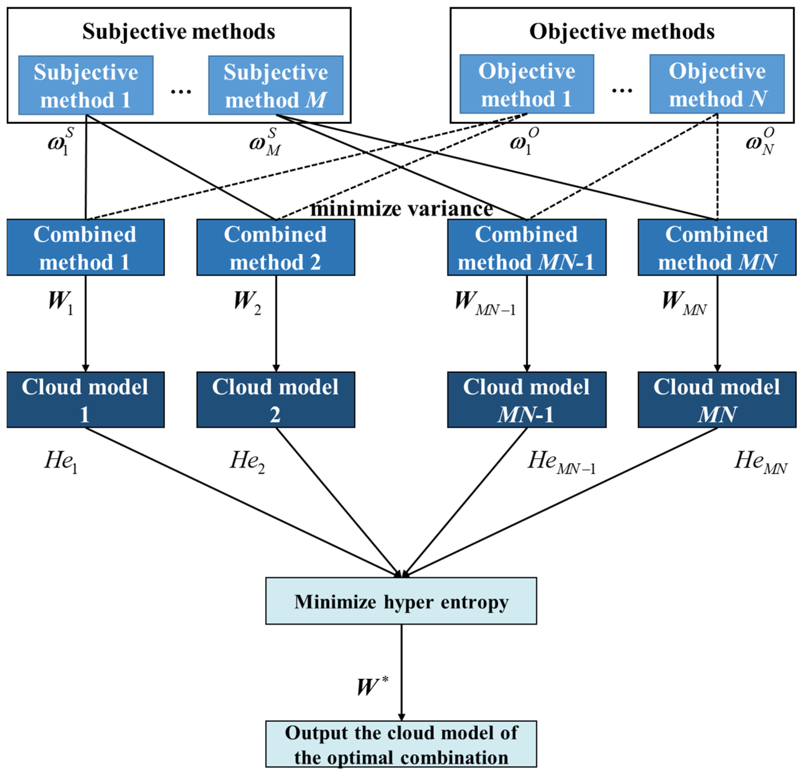
This paper uses the hyperentropy value to describe the rationality of the index weight cloud. The more concentrated the cloud drops are, the smaller the randomness of the membership degree of the rationality of the index weights, indicating that the combined weight is more reasonable. Therefore, the combination scheme with the smallest hyperentropy value is selected as the optimal combination. The combined weighting framework based on the minimum hyperentropy of the cloud model is shown in
Figure 1.
The proposed method is divided into the following steps:
Several different subjective and objective weight methods are applied to calculate the weights. Then, the index weight library is established by Equations (14) and (15).
where
and
represent the weights calculated by the
i-th subjective method and the
j-th objective method, respectively;
m and
n are the number of subjective and objective indices; and
M and
N are the number of subjective and objective weighting methods, respectively.
- 2.
Establish the index combination library and combined weight cloud.
To eliminate the bias of a single weighting method, this paper combines different subjective and objective weights in pairs to obtain MN combination schemes. Each combination’s weight is calculated based on the variance minimization approach.
First, the weights
and
are combined through a weighted linear combination to obtain the composite weight:
where
and
are the coefficients for subjective and objective weights, respectively, which satisfy
.
To obtain the optimal coefficients, the variance minimization is introduced to minimize the deviation of the linear combination of
from the set of weights
:
The optimal values of
and
can be derived by gradient calculation:
The final combined weight , k = 1, 2, …, MN of the subjective weight and the objective weight can be derived from Equation (16).
The weight cloud parameter
of the combined weight
is calculated as shown in Equations (19)–(21).
where
Wk,s is the
s-th element in the combination weight
.
- 3.
Select the optimal rational combined weights.
In the cloud model, the smaller the value of hyperentropy, the better the rationality of the index weights. Therefore, the set of weights with the smallest hyperentropy among all combinations is the optimal combination, denoted as .
4.3. Comprehensive Reliability Evaluation Model Based on Shortest Wasserstein Distance
In this paper, the reliability level of power systems is standardized into five levels. The risk intervals are estimated according to a 100-point scale, as shown in
Table 3. Here,
Cmin and
Cmax denote the lower and upper bounds of these reliability intervals, respectively.
Standard cloud models are established for these five levels, with the following numerical characteristics:
where the subscript
v represents reliability classes I to V and
k denotes a given value of hyperentropy.
A cloud model for the optimal combination is established. Using a bottom-up strategy, the cloud model parameters for all the indices can be calculated. Firstly, the parameters for each secondary index are determined based on the subjective and objective data. The optimal parameters (
Ex2,j,
En2,j,
He2,j) are similar to Equations (19)–(21), where the sample elements are replaced by the combination weights
of the evaluation results of each index
Aj,d. Based on the cloud model of the secondary indices, the cloud model of the CREI is obtained by following equations:
where
,
, and
are the mean expectation, entropy and hyperentropy of the cloud model, respectively.
Similarly, to calculate the cloud model parameters for each primary index, all secondary index data in Equations (25)–(27) can be replaced with the secondary index data under that primary index.
Finally, the developed cloud model is compared with the standard clouds. The Wasserstein distance between the models is calculated, and the standard cloud with the closest distance to the CREI cloud is selected as the evaluation result. In this paper, the distance between two cloud models is calculated by the following steps:
Each cloud drop is characterized by the expectation value
Ex, entropy
En, and hyperentropy
He. For the
v-th standard cloud, the entropy sample
Env,s (
s = 1, 2, …,
S) is generated based on
. Next, the expectation value sample
Exv,s is generated based on
. Similarly, the expectation value sample from the CREI cloud is denoted as
Exop,s. The membership degree of this sample is calculated as follows:
- 2.
Sort the expectations of cloud drops in ascending order, denoted as and , with elements denoted as and .
- 3.
Calculate the distances as follows:
After calculating the distance Dv (v = Ⅰ, …, Ⅴ) between the CREI cloud and the five standard clouds, the one with the smallest distance is selected as the result of the CREI.
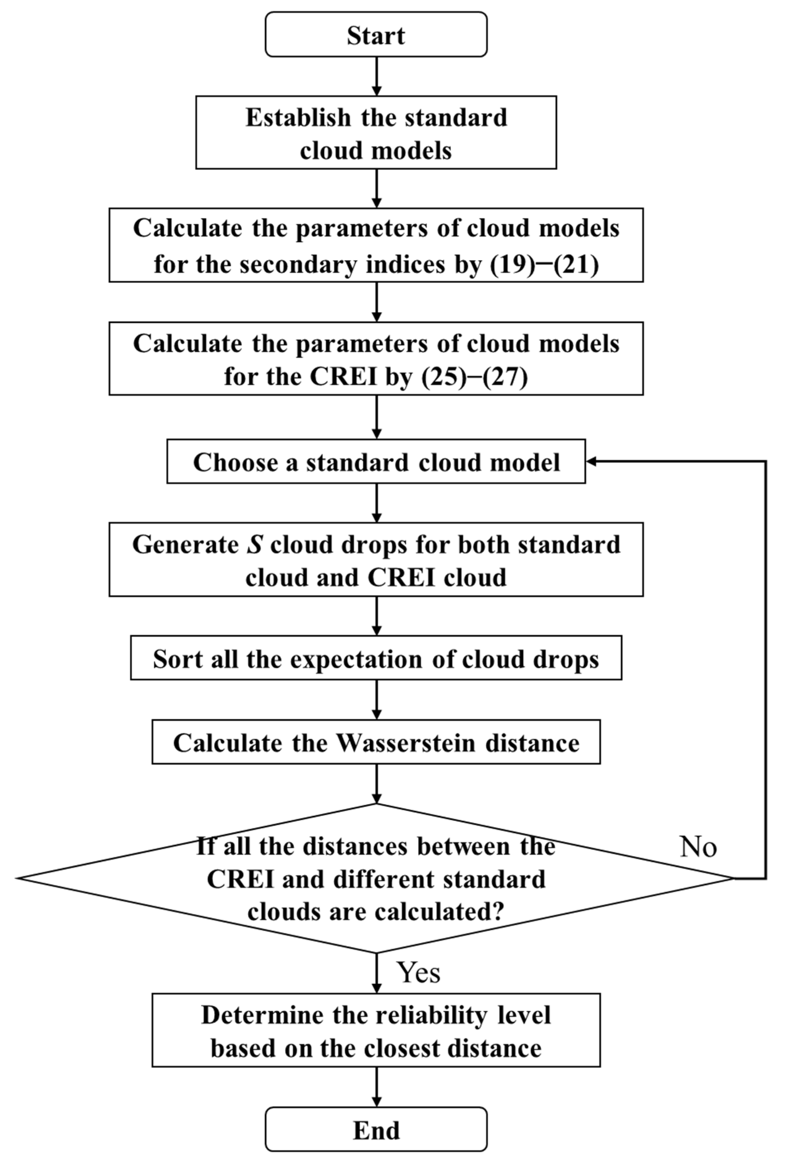
The flowchart of the comprehensive reliability evaluation method based on the cloud model is shown as
Figure 2. Initially, standard cloud models representing the worst, poor, middle, good, and best levels are established to serve as the benchmark for subsequent comparisons. Then, using the Equations (19)–(21), the
Ex,
En, and
He parameters for the cloud models of all the secondary indices are calculated, where the sample elements are replaced by the combination weights
Wk of the evaluation results of each index
Aj,d. Next, the three parameters of the cloud model for the CREI are determined. After obtaining the CREI cloud, the distance
Dv between the CREI and the five standard clouds are calculated as follows. For each comparison, one standard cloud model is chosen, and
S cloud drops are generated to represent its samples. They are then sorted in ascending order of their expected values. The distance is calculated by Equation (29). When all five distances are calculated, choose the smallest distance as the final result. Hence, the evaluation result of the CREI corresponds to the level indicated by the standard cloud associated with the minimum distance
Dv.
5. Case Study
In this paper, power grids of two cities in a province in Southern China are used to verify the proposed method. City A, the capital city of the province, features a more diversified power generation structure and advanced grid infrastructure. City B, an industrial hub of the province, hosts well-developed metallurgical and chemical industries. While power generation in City B is dominated by traditional energy sources, the city has begun to develop new energy sources in recent years.
This paper uses both subjective and objective weighting methods to calculate these secondary indices. Without loss of generality, for subjective indices, the fuzzy analytical hierarchy process (FAHP) [
38], Delphi method [
39], and best–worst method (BWM) [
40] are used. For objective weighting, the entropy weight method (EWM) [
41], variation coefficient method (VCM) [
42], and CRITIC method [
43] are adopted. Subjective data are obtained from experts and professors, while objective data are derived from real-world power grid data of the two cities. In the standard cloud models,
k is defined as
k =
Env/10 [
44].
According to the framework in
Figure 1,
Table 4 lists the hyperentropy values for the nine combination schemes. The combination method with the minimum hyperentropy is a combination of the FAHP and VCM methods. This indicates that the combined weighting method using FAHP and VCM is the most reasonable one for the research object of this paper.
Based on the combined weighting of FAHP and VCM, this paper calculates the weights of all indices in REIS and establishes their corresponding cloud models. The results for City A are summarized in
Table 5. Cloud models for primary indices and the CREI of the two cities are derived. The Wasserstein distances between these indices and the standard clouds are presented in
Table 6 and
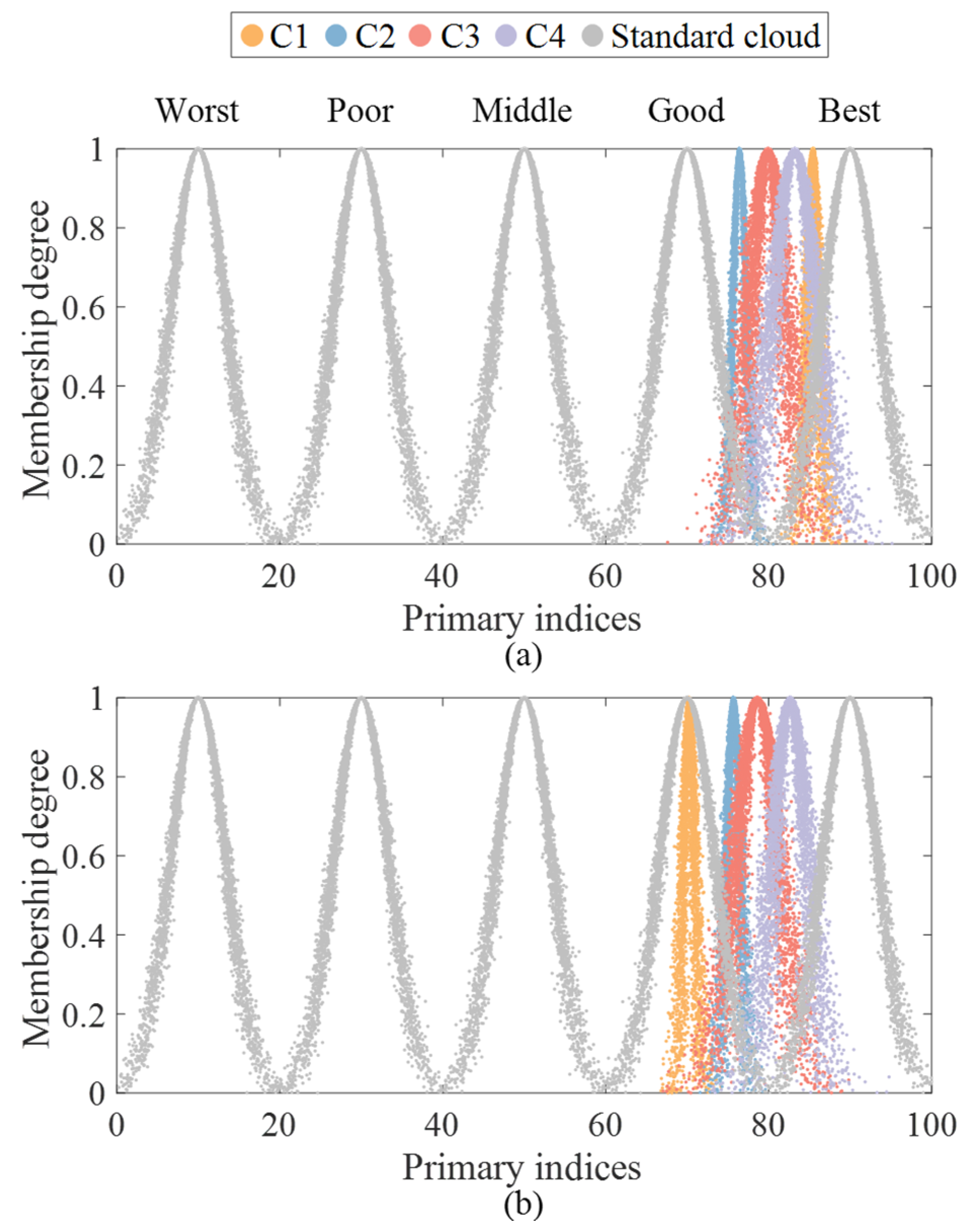
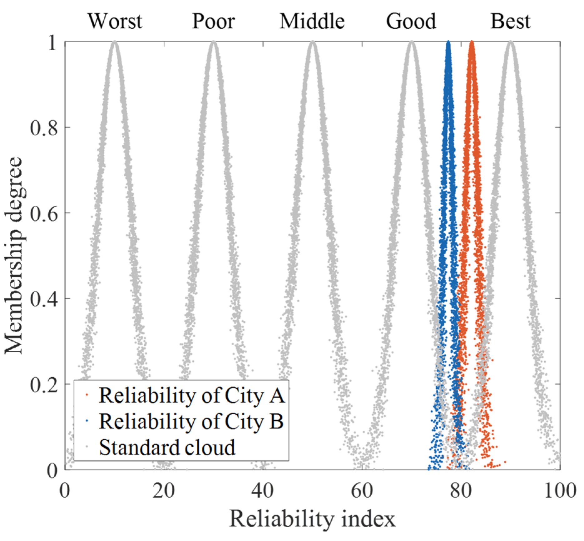
Table 7. The evaluation results of the cloud models for the primary indices and the CREI are illustrated in
Figure 3 and
Figure 4, respectively.
As shown in
Table 5, the CREI of City A is most closely related to reliability statistics
C4. In contrast, the flexibility of power systems contributes the least to reliability, with a weight of only 13.47%. Among all the secondary indices, the static voltage stability reserve coefficient
C13 and the static power angle stability reserve coefficient
C14 have the least impact on the CREI. Conversely, the average customer load not supplied
C44 has a significant impact on the CREI.
In addition, for stability C1, the static voltage stability reserve coefficient C13 ranks the lowest, while the system equivalent inertia C15 achieves the highest rating. Concerning generating capacity C2, renewable energy penetration C22 has the lowest score, whereas the inflow level in major river basins C24 is rated the highest. For flexibility C3, the hydropower unit equivalent ramp C33 is rated the lowest, but both the demand response participation level C34 and the load management execution capability C35 are rated the highest. Regarding the system reliability statistics, the average customer load not supplied C44 has the lowest rating, while the average customer load not supplied C42 is rated the highest.
According to
Table 6, the comprehensive evaluation results shows that City A excels in the stability, flexibility, and reliability statistics indices, all rated as “best.” The generation capacity, however, is rated as “good.” Consequently, the CREI for City A is “best.” Despite these high ratings, the results reveal specific weaknesses in City A’s grid, notably in generation capacity, particularly in renewable energy penetration
C22 and coal stockpile warning days
C23. To further enhance the reliability of the grid, it is recommended to prioritize improvements in generation capacity.
In
Table 7, City B’s grid is evaluated as “best” for both flexibility and reliability statistics, but only “good” for stability and generating capacity. The CREI for City B is also rated “good.” This suggests that while the grid performs well in some aspects, targeted improvements in stability and generating capacity are necessary to elevate the reliability level of City B’s grid.
By comparing the Wasserstein distances in
Table 6 and
Table 7, it can be concluded that City A outperforms City B in stability, flexibility, and reliability statistics. In contrast, City B has a slight advantage in generating capacity. The largest difference between the two cities is in the stability index and the smallest difference is in the generation capacity. Similar conclusions can be drawn from
Figure 3. Moreover, it can be seen from
Figure 4 that the reliability of the City A’s grid is stronger than that of City B. Therefore, the provincial grid company’s needs should prioritize improvements in City B to enhance the reliability of the provincial grid.
Moreover, to validate the accuracy of the proposed method, the reliability of the two cities can also be compared through other methods. Three methods are used: technique for order preference by similarity to ideal solution (TOPSIS) [
45], VIKOR [
46,
47], and grey relational analysis (GRA) [
48]. The evaluation results are listed in
Table 8,
Table 9 and
Table 10.
As the tables show, the reliability level of city A was higher than that of city B in all three methods. It indicates the correctness of the proposed method.
6. Conclusions
This paper establishes a reliability evaluation index system (REIS) and proposes an evaluation method to comprehensively evaluate the reliability of power systems with high penetration of renewable energies. Based on the analyses of some major blackout incidents in recent years, a three-hierarchy REIS is constructed. The top hierarchy is the comprehensive reliability evaluation index (CREI), which serves as an overall measure of system reliability. The middle hierarchy comprises four primary indices: stability, generation capacity, flexibility and system reliability statistics. The bottom hierarchy includes some specific secondary indices for each primary index.
To quantify the overall impact of each index on reliability, this paper proposes a combined weighting framework that selects the optimal combination from a variety of subjective and objective weighting methods according to their hyperentropy in weight cloud models. Five standard clouds, representing the worst, poor, middle, good, and best reliability levels, are constructed to quantify the reliability level of power systems. Based on the evaluation results of the secondary indices, cloud models for primary indices and the CREI are developed. Finally, the reliability level is determined by selecting the standard cloud with the closest Wasserstein distance to the CREI cloud.
The proposed method is particularly suitable for highly informatized power systems with substantial renewable energy integration. Its implementation primarily relies on data from advanced information systems (e.g., supervisory control and data acquisition, and phasor measurement units) and operational strategy records from grid operators, which can ensure adaptability to real-time system dynamics.
This paper illustrates the practicality of the proposed method by two city grids in a province in Southern China. The results indicate that, as an industrial hub of the province, the CREI of City B is on the second level, which is inferior to that of the provincial capital, City A. Therefore, to enhance the overall reliability of the province, the provincial grid company should prioritize improving the system reliability of City B, especially focusing on the stability and generation capacity, to reduce the potential risks.


 ,
, 
