Optimal Scheduling of Networked Microgrids Considering the Temporal Equilibrium Allocation of Annual Carbon Emission Allowance

Abstract

The optimal scheduling of networked microgrids considering the coupled trading of energy and carbon emission allowance (CEA) has been extensively studied. Notably, the scheduling is performed on a daily basis, whereas the CEA is usually checked and determined once a year. The temporal mismatch between the daily scheduling and the yearly CEA should be addressed to realize the dynamic valuation of CEA. In this paper, the optimal scheduling of networked microgrids considering the temporal equilibrium allocation of annual CEA is investigated. Firstly, a CEA decomposition model is developed, which allocates allowance to individual microgrids and further decomposes them temporally using the entropy method. Secondly, a Lyapunov optimization-based low-carbon scheduling model is introduced to manage carbon emissions within each dispatch interval, ensuring annual CEA compliance and daily economic efficiency. Thirdly, a Stackelberg game-based energy–carbon coupling trading model is presented, which considers the uncertainties caused by fluctuations in external electricity and carbon prices to optimize trading prices and strategies of the microgrids. Finally, a test system is used to demonstrate the significant effects of emission reduction and the economic benefits of the proposed methods.

1. Introduction

According to the Intergovernmental Panel on Climate Change (IPCC) report, global carbon emissions must be reduced by 45% from 2010 levels by 2030 to limit global warming to 1.5 °C [1]. Countries around the world are trying to stride toward the goal of carbon emission reduction [2]. To promote carbon emission reduction, the growing demand for clean energy transitions has become increasingly significant [3]. The integration of distributed renewable energies, in turn, has encouraged the development of microgrids, in which the energy is generated and consumed.

Nowadays, it has become a common practice to schedule the microgrid with carbon emission as a concern. Many carbon-oriented scheduling models have been proposed for the microgrid. In reference [4,5], the carbon emissions-related cost was added to the objective function to limit the system’s carbon emissions. In reference [6], a multi-objective optimization model for microgrids was established, which balances carbon emissions and economic benefits. Reference [7] proposed an energy management strategy considering carbon emissions constraint, which aims to limit the total carbon emissions of the microgrid within a given cap.

Moreover, carbon pricing has been recognized as an effective mechanism for realizing the collaborative operation of networked microgrids through financial incentives. Among the different options, the cap-and-trade system (also called carbon emission allowance (CEA) trading) prices the CEA based on the supply-demand equilibrium and reflects the time-varying scarcity of the allowance. Consequently, the cap-and-trade system has become one of the most prominent options for carbon pricing in industry practices. References [8,9] used a ladder-type carbon price model to set different carbon prices for different allowance trading intervals, which charges higher prices for more emissions to limit the carbon emissions. In reference [10], a differentiated dynamic pricing mechanism is considered for joint optimal dispatch of multi-energy microgrids.

Another advantage of the cap-and-trade system is that it is easily integrated within the energy trading structure. Moreover, the potential benefits of coupled trading of energy and CEA have been demonstrated in terms of securing profits and reducing emissions. In this area, many studies have been conducted. Reference [11] proposed a nodal energy–carbon price strategy, integrating carbon emission factors into the energy pricing models for integrated energy systems, aiming to reduce the costs and carbon emissions. Reference [12] proposed a hierarchical electricity and carbon coupling trading mechanism, which can measure carbon emissions, price electricity and carbon emissions at the distribution level, and increase prosumers’ profits.

Despite the aforementioned valuable research studies, a significant issue regarding the coupled trading of energy and CEA remains unaddressed. In accordance with the daily scheduling of the microgrids, it is common to perform the coupled trading of energy and CEA on a daily basis. However, it should be noted that the CEA for each utility is usually checked and determined once a year [13]. Therefore, a single microgrid has two ways to balance its carbon emission and the allowance, i.e., trade the CEA and control the carbon emission in the following days. Under such circumstances, it is hard for the microgrid to determine how much CEA it should buy or sell on a particular day. In other words, the coupled trading of energy and CEA is not only an optimization problem to balance economic benefits and carbon reduction but also a temporal equilibrium problem. Nevertheless, the temporal coupling issue has not been reported before.

To fill the research gap, the optimal scheduling of networked microgrids considering the temporal equilibrium allocation of annual CEA is investigated in this paper. Firstly, a method of allocating the total CEA to each microgrid and then to each day is analyzed. In this field, reference [14] proposes a rolling horizon optimization strategy for initial CEA in the power industry, utilizing a Stackelberg game model to decouple carbon trading from electricity markets, thereby optimizing emission reductions and power generation across multiple regions in China. In reference [15], a reasonable inter-provincial CEA scheme is proposed to obtain a reasonable CEA scheme that considers the contribution of the clean energy output. However, these studies only concerned the spatial allocation of CEA and did not consider the temporal mismatch between the daily scheduling and the yearly CEA, which could lead to annual cumulative carbon emissions exceeding allowance, resulting in penalties. Reference [16] introduced a seasonal carbon trading mechanism model. Although it shortened the time scale, it did not adequately consider uncertainties in renewable energy output and user load. In reference [17], a low carbon economic dispatching model with multi-time-scale allocation of CEA is proposed, redistributing CEA on an annual, monthly, and daily basis. However, it cannot address the impacts of carbon price fluctuations.

Secondly, a Lyapunov optimization-based scheduling model is analyzed. Lyapunov optimization is a powerful method used to solve long-term optimization problems in systems with random dynamics. It decomposes the original problem into a series of short-term subproblems that can be solved sequentially, with the solutions used to determine the optimal scheduling decisions for each time slot [18]. This approach allows for real-time decision-making without requiring prior knowledge of future states. Reference [19] details the application of Lyapunov optimization in a microgrid with distributed storage devices, where an aggregator controls the storage queues to provide ancillary services to a larger grid. However, it did not explicitly consider carbon emissions in the scheduling process, which is a crucial aspect in the context of low-carbon energy systems.

Thirdly, the coupled trading of energy and CEA between the distribution network operator (DNO) and microgrids (MGs) is analyzed. In this area, several studies have introduced various game theory frameworks to characterize multiple entities’ energy–carbon coupling trading behavior. In reference [20], an electricity–carbon integrated P2P market based on multi-leaders multi-followers (MLMF) Stackelberg game is proposed, which can reflect the relationship between prices and prosumers’ operation strategies. Reference [21] proposed an energy–carbon sharing method based on the Stackelberg game for the energy–carbon sharing and trading of the energy service provider and multiple integrated energy systems. In reference [22], a cooperative game model is proposed to maximize the profits of each entity while achieving carbon reduction via electricity and carbon trading. However, the aforementioned studies fail to adequately account for the uncertainties caused by external electricity and carbon price fluctuations.

In comparison, the Cournot model has also been widely used in modeling competition and market interactions, particularly in oligopolistic settings. In the context of energy markets, the Cournot model assumes that each player independently chooses its output quantity to maximize profit, considering the expected output of other players. The model has been applied to scenarios where firms or entities compete in terms of the amount of energy or carbon allowances they trade in the market, as seen in references [23]. The primary advantage of the Cournot model is its relative simplicity and its ability to model non-cooperative behavior when participants have little information about their competitors’ actions. However, unlike the Stackelberg model, where one player (the leader) makes the first move, the Cournot model assumes a simultaneous decision-making process, which may not fully capture the hierarchical structure observed in real-world energy and carbon markets.

Based on the discussion above, the innovative contributions of this paper can be summarized as follows:

(1)

A CEA temporal decomposition model is proposed. It allocates allowance to individual microgrids and further decomposes them temporally using the entropy method, thus providing a basis for daily scheduling.

(2)

A Lyapunov-optimization-based low-carbon scheduling model is proposed. It breaks down the annual CEA targets into each dispatch interval for management, avoiding penalties due to excessive emissions during annual settlement and ensuring both annual CEA compliance and daily economic efficiency.

(3)

A Stackelberg game-based energy–-carbon coupling trading model is presented. Moreover, it fully considers the uncertainty caused by external electricity and carbon price fluctuations, coordinating the electric–carbon coupling trading of the networked microgrids.

The remainder of this paper is organized as follows. Section 2 provides the framework of the carbon emission management and CEA temporal decomposition model. Section 3 presents the Lyapunov optimization-based low-carbon scheduling model. Section 4 establishes the energy–carbon coupling trading model of DNO and MGs, and the genetic algorithm is used to solve it. Section 5 provides case study results. Finally, conclusions are drawn in Section 6.

2. Carbon Emission Allowance Temporal Decomposition Model

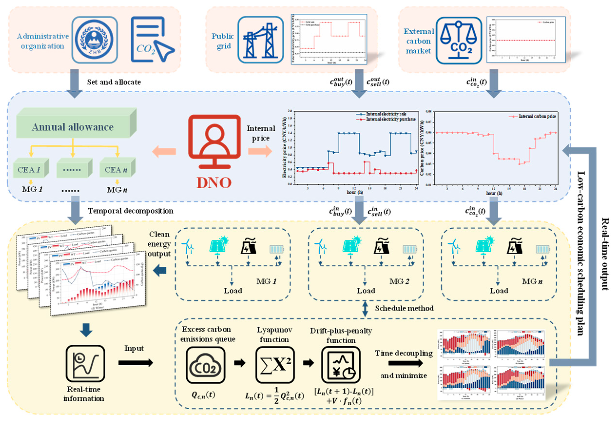
2.1. Framework for Carbon Emission Management

As demonstrated in Figure 1, a carbon emission management framework is proposed to ensure both annual CEA compliance and daily economic efficiency of MGs.

The target users of carbon emission management are DNOs and MGs, which are electricity-dependent and have significant potential for carbon reduction. MGs are equipped with distributed photovoltaic, wind turbine, thermal power generation, energy storage units, and energy management systems (EMSs). An EMS is used to transmit information between DNOs and MGs. Because of the entry barriers of the CEA trading, in practice, some MGs are not eligible to participate in CEA trading [24]. In this paper, the DNO aggregates these MGs to reach the barriers and obtain CEA from the administrative organization.

It can be seen that there is mainly a pricing stage in the upper layer and a scheduling stage in the lower layer. The DNO is a bridge between the public grid and MGs, which purchases and sells electricity externally and meets the load demands of the MGs to balance the relationship between supply and demand. The DNO also allocates CEA obtained from the administrative organization to individual microgrids and trades with the external carbon market to meet the CEA demands of MGs. While developing price strategies, the DNO should consider the external price range to prevent direct electricity transactions between MGs and the public grid. In addition, in the transaction process between the DNO and MGs, it is necessary to take responsibility for the imbalance in supply and demand. If the supply and demand balance is not met, purchasing electricity or CEA from the public grid or external carbon market is necessary.

For the upper and lower optimization models, the optimization result of one layer is the input of another layer. The DNO first formulates the internal price strategy according to external prices and MGs’ demands. The MGs accept the price set by the DNO to formulate a low-carbon economic scheduling plan, which includes the output of equipment and electricity and CEA trading strategies. The optimization process between the DNO and MGs is sequential, which conforms to the game situation of the master–slave architecture. Therefore, this paper adopts the Stackelberg game model to deal with the corresponding two stages.

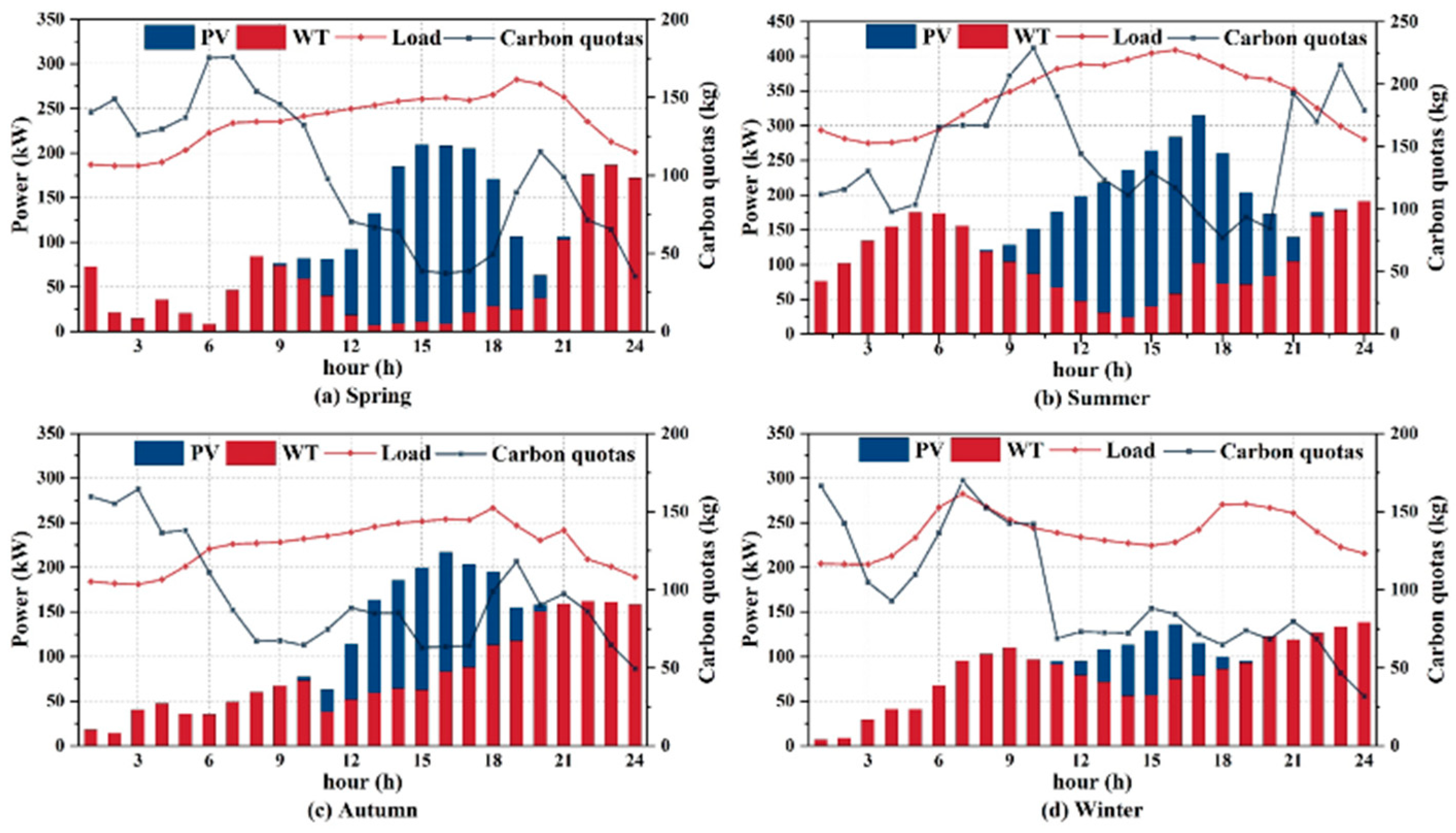
2.2. Temporal Decomposition of Carbon Emission Allowances

After obtaining CEA from the DNO, MGs perform temporal decomposition of the CEA. Three temporal decomposition indicators were established in reference to spatial allocation indicators [25]. The indicators are shown in

Table 1. Temporal decomposition indicators for CEA.

Indicator	Explanation	Attribute
Historical carbon emissions	Ensure sufficient allowances during periods of high carbon emissions	+
Historical clean energy generation	Reduce the use of CEA during periods of abundant clean energy	−
Seasonal adjustment factor	Adjust the usage of CEA according to the seasonal characteristics of the load	+

.

The indicators in Table 1 are established from the MGs’ perspective. This process aims to allocate CEA more reasonably across different periods. The indicators are divided into positive and negative categories, represented by “+” and “−”. The larger the positive indicator, the more allowances are allocated; conversely, the larger the negative indicator, the fewer allowances are allocated.

The entropy method is used to set weight based on the amount of information from the indicators to eliminate the influence of subjective factors. Assuming the value of the n-th indicator of the m-th day is x_mn (m = 1, …, 365; n = 1, …, 3), the steps for assigning weights using the entropy method are as follows.

Firstly, the data are normalized. Historical carbon emissions and seasonal adjustment factors are positive indicators, which means that the larger the value is, the more allowance ought to be assigned. The positive indicator can be standardized as follows:

$$r_{mn}={\displaystyle \frac{x_{mn}-{\min }_m{x}_{mn}}{{\max }_m{x}_{mn}-{\min }_m{x}_{mn}}}$$

(1)

where $r_{mn}$ is the normative value of the n-th indicator of the m-th day; ${\min }_m{x}_{mn}$ and ${\max }_m{x}_{mn}$ are the maximum and minimum values of the n-th indicator, respectively.

The historical clean energy generation is a negative indicator, which means that the larger the value is, the fewer allowances should be assigned. The negative indicator can be standardized as

$$r_{mn}^{\prime }={\displaystyle \frac{{\max }_m{x}_{mn}-x_{mn}}{{\max }_m{x}_{mn}-{\min }_m{x}_{mn}}}$$

(2)

where $r_{mn}^{\prime }$ is the normative value of the n-th indicator of the m-th day. $r_{mn}$ and $r_{mn}^{\prime }$ are the normative values of positive and negative indicators, respectively, collectively referred to $R_{mn}$:

$$R_{mn}=\left\{\begin{array}{l}{r}_{mn}, n=1,3\\ r_{mn}^{\prime }, n=2\end{array}\right.$$

(3)

The ratio of $R_{mn}$ to the sum of 365 days of the n-th indicator ($p_{mn}$) is calculated as follows:

$$p_{mn}={\displaystyle \frac{R_{mn}}{{\displaystyle \sum _{m=1}^{365}}{R}_{mn}}}$$

(4)

Secondly, the entropy value of each indicator can be computed as

$$e_n=-{(\ln 365)}^{-1}\sum _{m=1}^{365}[p_{mn}\ln (p_{mn})]$$

(5)

where $e_n$ is the information entropy of indicator n, if $p_{mn}=0$; $p_{mn}\ln (p_{mn})=0$. Smaller information entropy means that the indicator carries more information, and more useful information can be obtained.

Thirdly, the weight of each indicator can be computed. The weight of the n-th indicator ($w_n$) is

$$w_n={\displaystyle \frac{1-e_n}{{\Sigma }_{n=1}^3(1-e_n)}}$$

(6)

Fourthly, the comprehensive index of the m-th day ($I_m$) is constructed according to $w_n$ as follows:

$$I_m={\displaystyle \sum _n{w}_n{p}_{mn}}$$

(7)

Fifthly, the weight of temporal decomposition for CEA for the m-th day ($v_m$) can be obtained by the following formula:

$$v_m={\displaystyle \frac{I_m}{{\Sigma }_{m=1}^{365}{I}_m}}$$

(8)

Finally, the CEA for the m-th day ($A_{Day,m}$) after temporal decomposition can be obtained as follows:

$$A_{Day,m}=C_{Year}\times {\nu }_m$$

(9)

3. Lyapunov Optimization-Based Low-Carbon Scheduling of the Microgrid

In this section, a Lyapunov optimization-based low-carbon scheduling model is proposed to establish a low-carbon economy scheduling plan. Lyapunov optimization uses a Lyapunov function to control a dynamical system. The proposed model does not require any predicted information about the output of clean energy generation or price and can be implemented easily as an online algorithm.

3.1. Actual Carbon Emissions

The carbon emission in MGs mainly includes thermal power inside and electricity buying from the external [26]. The actual carbon emission model is as follows:

$$E_{e,n}(t)=E_{buy,n}(t)+E_{g,n}(t)$$

(10)

$$E_{buy,n}(t)={\delta }_{buy}\cdot P_{buy,n}(t)$$

(11)

$$E_{g,n}(t)={\delta }_g\cdot P_{g,n}(t)$$

(12)

where $E_{e,n}(t)$ is the actual carbon emissions of MG n in period t. $E_{buy,n}(t)$ and $E_{g,n}(t)$ are the actual carbon emissions of the electricity purchased from the external, thermal power generation of MG n in period t, respectively; ${\delta }_{buy}$, ${\delta }_g$ denote the carbon emission intensity of external grid generation and thermal power generation, respectively; $P_{buy,n}(t)$ is the power purchased from the external of MG n in period t; $P_{g,n}(t)$ is the output of thermal power generation of MG n in period t.

3.2. Lyapunov Optimization-Based Low-Carbon Economic Scheduling Model

Lyapunov optimization was first introduced to optimize the management of queueing systems. It aims to balance system performance and queue congestion [27]. The cumulative excess carbon emissions can be considered as a queue backlog. The goal of Lyapunov optimization in this paper is to maintain a good balance between CO₂ over-emissions and operating costs.

To fit our problem into the Lyapunov optimization framework, a cumulative excess carbon emission queue is defined as

$$Q_{c,n}(t+1)=Q_{c,n}(t)+E_{e,n}(t)-A_{m,n}(t)$$

(13)

where $Q_{c,n}(t+1)$ and $Q_{c,n}(t)$ represent the cumulative CO₂ over-emission of MG n at period t + 1 and period t. $A_{m,n}(t)$ is the allowance amount invested by MG n at period t, which is decomposed again by the daily CEA $A_{Day,m}$.

Then, according to the typical Lyapunov optimization framework [28], a quadratic Lyapunov function $L_n(t)$ is defined as

$$L_n(t)=L(Q_{c,n}(t))\triangleq {\displaystyle \frac{1}{2}}{Q}_{c,n}^2(t)$$

(14)

It is evident that the Lyapunov quadratic function is non-negative. Then, the single-slot conditional Lyapunov drift $\Delta L_n(t)$ is defined as

$$\Delta L_n(t)\triangleq L_n(t+1)-L_n(t)$$

(15)

The Lyapunov drift indicates the expected difference in the Lyapunov function from one slot to the next under the current state. It is clear that the minimization of the Lyapunov drift at each time slot results in a lower congestion state of the backlogs, which intuitively maintains network stability [29]. In this paper, it means the reduced chance of successive increases of the excess emissions of CO₂.

After introducing the cumulative excess carbon emissions queue, the goal becomes to find an economical scheduling plan while maintaining the virtual queue stability. To achieve the dual goals, the drift-plus-penalty function is introduced by adding the cost function of the traditional low-carbon economic scheduling model to the Lyapunov drift:

$$F_n(t)=\Delta L_n(t)+V\cdot f_n(t)=L_n(t+1)-L_n(t)+V\cdot f_n(t)$$

(16)

where $F_n(t)$ is the drift-plus-penalty function of MG n at period t, and V is a weight parameter to balance the operating cost and the queue stability. The cost function $f_n(t)$ is computed as

$$f_n(t)=f_{g,n}(t)+f_{e,n}(t)+f_{c,n}(t)$$

(17)

$$f_{g,n}(t)=a_n{P}_{g,n}^2(t)+b_n{P}_{g,n}(t)+c_n$$

(18)

$$f_{e,n}(t)=P_{sell,n}(t)\cdot c_{buy}^{in}(t)-P_{buy,n}(t)\cdot c_{sell}^{in}(t)$$

(19)

$$f_{c,n}(t)=(E_{e,n}(t)-A_{m,n}(t))\cdot c_{co2}^{in}(t)$$

(20)

where $f_{g,n}(t)$, $f_{e,n}(t)$ and $f_{c,n}(t)$ are the cost of thermal power generation, electricity trading, and CEA trading of MG n at period t, respectively; $a_n$, $b_n$, $c_n$ are relevant parameters. $P_{sell,n}(t)$/$P_{buy,n}(t)$ are the power sold/purchased to/from DNO by MG; $c_{sell}^{in}(t)$/$c_{buy}^{in}(t)$ are the selling/purchase price of electricity to/from DNO at period t. $c_{co2}^{in}(t)$ is the carbon trading price set by DNO at period t.

However, it cannot directly minimize the drift-plus-penalty function because of the time-coupling item. To solve this problem, this paper calculates the upper bound of the drift-plus-penalty function as Theorem 1. The proof of Theorem 1 is presented in Appendix A.

Theorem 1. 

If the upper bound of the $E_{e,n}(t)$ and $A_{m,n}(t)$ are $E_{\max }$, $A_{\max }$, respectively, the drift-plus-penalty function satisfies the following inequality in all periods:

$$L_n(t+1)-L_n(t)+V\cdot f_n(t)\le B+Q_{c,n}(t)[E_{e,n}(t)-A_{m,n}(t)]+V\cdot f_n(t)$$

(21)

where B is a constant, which is calculated as

$$B={\displaystyle \frac{E_{\max }^2+A_{\max }^2}{2}}$$

(22)

The time-coupling item can be removed, and the objective function of the low-carbon scheduling model is denoted as follows:

$$F_{n,t}(t)=Q_{c,n}(t)[E_{e,n}(t)-A_{m,n}(t)]+V\cdot f_n(t)$$

(23)

The operational constraints of the low-carbon scheduling model are expressed as follows:

(1)

Energy storage equipment constraints:

$$0\le P_{char,n}(t)\le P_{cha,n}^{\max }\cdot B_{EES,char}(t),\hspace{1em}\forall t$$

(24)

$$0\le P_{dis,n}(t)\le P_{dis,n}^{\max }\cdot B_{EES,dis}(t),\hspace{1em}\forall t$$

(25)

$$0\le B_{EES,char}(t)+B_{EES,dis}(t)\le 1,\hspace{1em}\forall t$$

(26)

where $P_{char,n}(t)$ and $P_{dis,n}(t)$ are the charging and discharging power of the energy storage equipment in period t; $P_{cha,n}^{\max }$ and $P_{dis,n}^{\max }$ are the maximum charging and discharging power of the storage equipment; $B_{EES,char}(t)$ and $B_{EES,dis}(t)$ are the charging and discharging status of the storage equipment; $B_{EES,char}(t)=1$, $B_{EES,dis}(t)=0$ indicate the charge of the storage equipment; and $B_{EES,char}(t)=0$, $B_{EES,dis}(t)=1$ indicate the discharging of the storage equipment.

For the capacity limits of the storage equipment, if the same method is used for time-decoupling, the capacity limitations will constrain the values of the weight parameter V [29]. Therefore, in this study, this paper controls the energy storage equipment’s charging and discharging behavior based on time-of-use pricing and real-time battery state of charge [30].

(2)

Thermal power units and electricity trading constraints:

$$P_{g,n}^{\min }\le P_{g,n}(t)\le P_{g,n}^{\max },\hspace{1em}\forall t$$

(27)

$$0\le P_{sell,n}(t)\le B_{sell,n}(t)\cdot P_n^{Max},\hspace{1em}\forall t$$

(28)

$$0\le P_{buy,n}(t)\le B_{buy,n}(t)\cdot P_n^{Max},\hspace{1em}\forall t$$

(29)

$$0\le B_{sell,n}(t)+B_{buy,n}(t)\le 1,\hspace{1em}\forall t$$

(30)

where $P_{g,n}^{\max }$ and $P_{g,n}^{\min }$ are the maximum and minimum output values of the thermal power unit; $P_n^{Max}$ is the upper limit of the electricity trading value; $B_{sell,n}(t)$ and $B_{buy,n}(t)$ are the selling and purchasing status of the MG n at period t, $B_{sell,n}(t)=1$, $B_{buy,n}(t)=0$ indicate selling power to the DNO, and $B_{sell,n}(t)=0$, $B_{buy,n}(t)=1$ indicate purchasing power from the DNO.

(3)

Load balance constraint:

$$P_n(t)=P_{W,n}(t)+P_{PV,n}(t)-P_{char,n}(t)+P_{dis,n}(t)+P_{g,n}(t)-L_{E,n}(t)$$

(31)

where $P_{W,n}(t)$ and $P_{PV,n}(t)$ are the output power of the wind turbine and PV unit of MG n in period t; $L_{E,n}(t)$ is the load of the corresponding time period; $P_n(t)$ is the net load of MG n in period t, which is calculated as follows:

$$P_n(t)=P_{sell,n}(t)-P_{buy,n}(t)$$

(32)

Based on the above models, the Lyapunov optimization-based low-carbon scheduling model is formulated as

$$\begin{array}{l}\min Q_{c,n}(t)[E_{e,n}(t)-A_{m,n}(t)]+V\cdot f_n(t)\\ \mathrm{s}.\mathrm{t}. \left(10\right)-\left(12\right), \left(24\right)-\left(32\right)\end{array}$$

(33)

It is clear that the proposed model does not require any prior or prediction information about the price and output of clean energy generation. It seeks to maintain a balance between CO₂ over-emissions and operating costs and can be solved online.

4. Stackelberg Game-Based Energy–Carbon Coupling Trading Among the Microgrids

The Stackelberg game model is a strategic decision-making framework used to model situations where players make decisions sequentially rather than simultaneously. In this context, one player, the leader, makes a move first, and the other players, the followers, adjust their strategies based on the leader’s decision [31]. The Stackelberg model is particularly suited for modeling hierarchical sequential decision-making, where entities such as the distribution network operator (DNO) and microgrids (MGs) interact with asymmetric information and decision-making power. In our study, the DNO acts as the leader, setting the market price for both electricity and carbon, while the MGs follow and make their decisions accordingly.

4.1. The Framework of the Stackelberg Game

The framework of the Stackelberg game-based energy–carbon coupling trading is presented in Figure 2.

The DNO is the leader that maximizes its revenue, considering external electricity and carbon price constraints to set the internal electricity and carbon trading price. MGs are the followers that accept the price set by DNO. Meanwhile, the MGs formulate power and CEA consumption and equipment scheduling strategies by solving the scheduling model at each moment. The internal electricity price and carbon price determine the cost and transaction strategy of MGs, and the transaction strategy of MGs determines the revenue of the DNO. Therefore, the game between the two, in turn, constitutes the Stackelberg game.

The Stackelberg game model constructed in this paper includes the following parts:

(1)

Participants: the DNO and MGs form a Stackelberg game as leaders and followers, respectively.

(2)

Strategies: the DNO’s strategy is to set the internal electricity and carbon prices, and the MGs’ strategy is electricity and allowances transaction strategies.

(3)

Utility function: the DNO’s utility function is to maximize profit, and MGs’ utility function is to minimize the drift-plus-penalty function as a Formula (23).

4.2. The Revenue Model of DNO

In internal energy and CEA transactions, some MGs are sellers, and others are buyers. The DNO would promote electricity and allowances transactions between MGs by optimizing the internal electricity and CEA purchase and sale prices. Meanwhile, the DNO needs to maintain the supply and demand balance. When the power generation within the MG system is lower than the power consumption, the DNO needs to purchase electricity from the public grid. When the power generation within the MG system is higher than the power consumption, the DNO needs to sell electricity to the public grid for profit. The sold and purchased electricity can be calculated as follows:

$$P_{Esell}(t)={\displaystyle \sum _{B_{buy,n}=1}{P}_{buy,n}(t)}$$

(34)

$$P_{Ebuy}(t)={\displaystyle \sum _{B_{sell,n}=1}{P}_{sell,n}(t)}$$

(35)

where $P_{Esell}(t)$ and $P_{buy,n}(t)$ are the electricity sold to the MGs and the electricity purchased from the MGs at time t, respectively.

Similarly, when the CEA within the MG system is insufficient, the DNO needs to purchase CEA from the external carbon market. When the CEA within the MG system is surplus, the DNO needs to sell allowances to the external carbon market. The net CEA $A_{Tra}(t)$ is calculated as follows:

$$A_{Tra}(t)={\displaystyle \sum _{n\in N}{A}_{Tra,n}(t)}={\displaystyle \sum _{n\in N}(A_{m,n}(t)-E_{e,n}(t))}$$

(36)

According to the trading between the DNO, the MGs, the public grid, and the external carbon market, the optimization objective of the DNO can be expressed as

$$\max F_{op,t}(t)=\max [F_E(t)+F_C(t)]$$

(37)

$$\begin{array}{l}{F}_E(t)=P_{Esell}(t)\cdot c_{buy}^{in}(t)-P_{Ebuy}(t)\cdot c_{sell}^{in}(t)\\ -\min \{0,(P_{Esell}(t)-P_{Ebuy}(t)\}\cdot c_{sell}^{ex}(t)\\ -\max \{0,(P_{Esell}(t)-P_{Ebuy}(t)\}\cdot c_{buy}^{ex}(t)\end{array}$$

(38)

$$F_C(t)=(c_{co2}^{out}(t)-c_{co2}^{in}(t))\cdot A_{Tra}$$

(39)

where $F_{op,t}(t)$ is the utility function of the DNO in period t, $F_E(t)$ is the revenue from electricity trading, and $F_C(t)$ is the revenue from CEA trading. $c_{sell}^{in}(t)$ and $c_{buy}^{in}(t)$ are the selling/purchase price of electricity to/from the external grid. $c_{co2}^{out}(t)$ is the carbon trading price of the external carbon market.

In order to protect the benefits of the DNO and, at the same time, to prevent MGs from participating in transactions with the external grid, the following constraints must be satisfied:

$$c_{sell}^{out}(t)\le c_{sell}^{in}(t) < c_{buy}^{in}(t)\le c_{buy}^{out}(t)$$

(40)

$$c_{co2}^{\min }(t)\le c_{co2}^{in}(t)\le c_{co2}^{\max }(t)$$

(41)

where $c_{co2}^{\max }(t)$ and $c_{co2}^{\min }(t)$ are the maximum and minimum prices of CEA.

4.3. Formulation and Solution of Stackelberg Game Model

According to the above analysis, the Stackelberg game-based energy–carbon coupling trading can be described as

$$G_{stac}=\{(DNO\cup MGs);\{{\Phi }_{in,t}\};{\left\{{\Theta }_{n,t}\right\}}_{n\in MGs};F_{op,t};{\left\{F_{n,t}\right\}}_{n\in MGs}\}$$

(42)

where $(DNO\cup MGs)$ are the two participants in the Stackelberg game; $\left\{{\Phi }_{in,t}\right\}$ is the set of internal electricity and carbon trading prices at period t; ${\left\{{\Theta }_{n,t}\right\}}_{n\in MGs}$ is the set of electricity and CEA consuming strategies of MGs at period t.

According to Nash equilibrium, the condition for the model to have a game equilibrium point is that there is a strategy $({\Phi }_{in,t}^{*},{\Theta }_{n,t}^{*})$ in the strategy space that satisfies the following constraints:

$$F_{op,t}({\Phi }_{in,t}^{*},{\Theta }_{n,t}^{*})\ge F_{op,t}({\Phi }_{in,t},{\Theta }_{n,t}^{*}),\forall {\Phi }_{in,t}\in {\Phi }_{in,t}$$

(43)

$$F_{n,t}({\Phi }_{in,t}^{*},{\Theta }_{n,t}^{*})\le F_{n,t}({\Phi }_{in,t}^{*},{\Theta }_{n,t}^{*},{\Theta }_{-n,t}^{*}),\forall n\in MGs,{\Theta }_{n,t}^{*}\in {\Theta }_{n,t}^{*}$$

(44)

where ${\Theta }_{-n,t}^{*}$ is the optimal strategy set of other MGs except n. The Nash equilibrium point $({\Phi }_{in,t}^{*},{\Theta }_{n,t}^{*})$ is the model solution. Under this strategic combination, the DNO cannot unilaterally change the internal electricity and carbon price strategy to improve its revenue, and the MGs cannot reduce operating costs by unilaterally changing the electricity and allowance transaction and scheme. The proof of Stackelberg game equilibrium is presented in Appendix B.

The Stackelberg game model constructed in this paper involves the collaborative optimization of the upper and lower levels of subjects; each subject needs to optimize based on the information of the other variables. The upper layer, which involves decision-making for the DNO’s strategies, is a large-scale nonlinear optimization problem. To address this, we use a genetic algorithm, which helps reduce the computational complexity and enhances the optimization capability [32]. The lower layer, which involves the Lyapunov optimization-based scheduling model, is a linear model. This model can be conveniently solved using the Gurobi solver, a commercial optimization solver widely used for mixed-integer programming problems [33]. The specific solution steps are as follows:

• Step 1: The parameters of the DNO and MGs, k = 0, are initialized; the number of populations m is set to 10, the number of iterations to 30, the population variation rate to 5%, and the crossover probability to 70%. The choice of these parameters is based on previous studies, particularly [34], where similar settings have been found to provide effective results for optimization problems of this nature.
• Step 2: A genetic algorithm is used to randomly generate m sets of acceptable internal electricity prices and carbon prices for the MGs, the DNO calculates optimal revenue and sends the corresponding prices to the MGs.
• Step 3: k = k + 1.
• Step 4: If k = 30, the iteration is ended, and the optimal prices and scheduling plan are output; otherwise, step 5 is initialized.
• Step 5: MGs receive the optimal internal prices, using the Gurobi solver to solve the scheduling model. It calculates and retains the current operating cost $F_{n,t}(t)$ and returns its moment-by-moment electricity and allowance transaction strategy to the DNO.
• Step 6: The DNO calculates its current revenue $F_{op,t}(t)$ based on the electricity and allowance transaction information returned by MGs.
• Step 7: If convergence conditions are met, the iteration is ended and the optimal prices and scheduling plan are output; otherwise, step 8 is initialized.
• Step 8: The genetic algorithm’s selection and mutation are used to generate new internal prices and calculate the DNO’s revenue ${F_{op,t}(t)}^{\prime }$ based on new prices.
• Step 9: If ${F_{op,t}(t)}^{\prime }$ > $F_{op,t}(t)$, internal prices are updated and step 3 is resumed; otherwise, step 8 is resumed.

5. Case Analysis

Take a specific networked microgrid system including a DNO and three MGs in China as the research object. The typical four-season characteristics are selected and divided into 24 periods of 1 h. The external electricity price is displayed in Figure 3 [35]. The external carbon price is set to 0.04 CNY/kg [36]. The main scheduling parameters of the MG are shown in

Table 2. Parameter settings for the equipment in the proposed MGs.

Equipment	Parameter	Value
TP1	a1 (CNY/(kW2·h))	0.00475
	b1 (CNY/(kW·h))	0.3
	c1 (CNY/h)	12
	$P_g^{min}$ (kW)	20
	$P_g^{max}$ (kW)	400
TP2	a2 (CNY/(kW2·h))	0.00515
	b2 (CNY/(kW·h))	0.38
	c2 (CNY/h)	16
	$P_g^{min}$ (kW)	10
	$P_g^{max}$ (kW)	375
TP3	a3 (CNY/(kW2·h))	0.00515
	b3 (CNY/(kW·h))	0.4
	c3 (CNY/h)	18
	$P_g^{min}$ (kW)	10
	$P_g^{max}$ (kW)	425
EES1	$P_{cha}^{min}$ (kW)	20
	$P_{dis}^{max}$ (kW)	20
EES2	$P_{cha}^{min}$ (kW)	40
	$P_{dis}^{max}$ (kW)	60
EES3	$P_{cha}^{min}$ (kW)	35
	$P_{dis}^{max}$ (kW)	40
Grid	$P_n^{max}$ (kW)	200

.

5.1. Comparison of Different CEA Allocation Scheme and Scheduling Methods

In order to verify the feasibility of the CEA temporal decomposition model and Lyapunov optimization-based low-carbon scheduling model, this paper takes MG 1 without a DNO for analysis. The following three scenarios are set:

Scenario 1: The CEA is allocated through annual averaging. The MG schedules with the proposed Lyapunov optimization-based method, and the simulation duration is set to 24 h.

Scenario 2: The CEA is allocated through temporal decomposition. The MG schedules with the proposed Lyapunov optimization-based method, and the simulation duration is set to 24 h.

Scenario 3: The CEA is allocated through temporal decomposition. The MG dispatches with the traditional low-carbon economic scheduling method (offline optimization with complete information), and the simulation duration is set to 24 h.

The output of renewable energy sources, electricity daily load, and CEA after temporal decomposition is shown in Figure 4.

According to the above scenarios, the typical daily CO₂ over-emissions and operating costs of MG 1 in four seasons are shown in

Table 3. Operating costs and CO₂ over-emissions in Scenarios 1, 2 and 3.

Scenario		Spring	Summer	Autumn	Winter	Total
1	Operating costs (¥)	2802.4	3819.5	2412.3	3203.7	12,237.9
	CO2 over-emissions (kg)	720.1	706.2	534.8	1397.6	3358.7
2	Operating costs (¥)	2834.8	3701.4	2361.7	3130.8	12,028.7
	CO2 over-emissions (kg)	756.4	500.2	479.2	1278.9	3014.7
3	Operating costs (¥)	2526.8	3336.8	2029.8	2849.4	10,742.8
	CO2 over-emissions (kg)	913.4	607.9	694.5	1372.3	3588.1

.

Compared with Scenario 1, in Scenario 2, except for spring, the costs and CO₂ over-emissions in summer, autumn, and winter are all reduced, with costs reduced by 3.1%, 2.1%, and 2.3%, respectively, and CO₂ over-emissions reduced by 29.2%, 10.4%, and 8.5%, respectively. In spring, due to the abundant output of clean energy units and the lower load level of MG 1, the CEA decomposed in Scenario 2 is less than the average. Thus, the costs and CO₂ over-emissions are 1.1% and 5% higher than in Scenario 1. Regarding the total costs, Scenario 2 is 1.7% lower than Scenario 1, and the CO₂ over-emissions are reduced by 10.2%. After implementing the temporal decomposition of CEA, the MG can effectively reduce excessive CO₂ emissions and reduce costs to a certain extent.

Compared with Scenario 3, the CO₂ over-emissions in the typical days of four seasons in Scenario 2 are reduced by 17.2%, 17.7%, 31%, and 6.8%, respectively. The total CO₂ over-emissions in Scenario 2 are reduced by 16.0%. This illustrates that the proposed method can reduce carbon emissions effectively. Meanwhile, the dynamic energy balance of the MG is analyzed in Scenarios 2 and 3, as shown in Figure 5 and Figure 6. In Scenario 3, the MG chooses to charge the energy storage equipment during valley hours while discharging during peak hours; therefore, the total cost of Scenario 3 is 10.7% lower than Scenario 2.

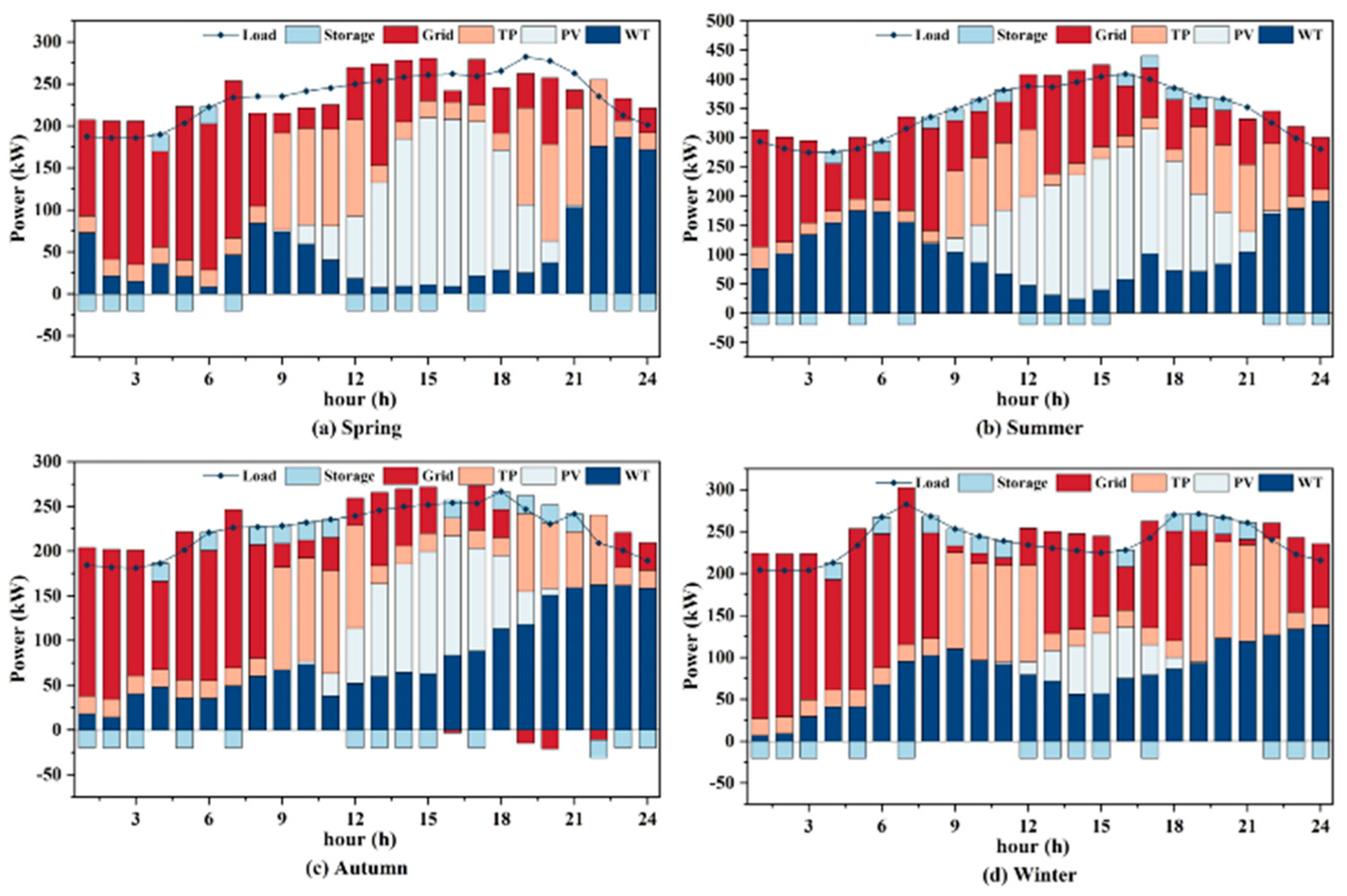
5.2. Analysis of Long-Term Economic Benefits

In order to investigate the long-term economic benefits of the proposed low-carbon scheduling method, the simulation duration is extended to 168 h (Scenario 4 and 5) as follows:

Scenario 4: The CEA is allocated through temporal decomposition. The MG schedules with the proposed Lyapunov optimization-based method, and the simulation duration is set to 168 h.

Scenario 5: The CEA is allocated through temporal decomposition. The MG schedules with the traditional low-carbon economic scheduling method (offline optimization with complete information), and the simulation duration is set to 168 h.

The optimization results of these two scenarios are shown in

Table 4. Operating costs and CO₂ over-emissions in Scenarios 4 and 5.

Scenario		Spring	Summer	Autumn	Winter	Total
4	Operating costs (¥)	14,523.8	44,544	20,720.8	22,600.7	102,389.3
	CO2 over-emissions (kg)	1560.1	11,606.5	2091.5	5081.9	20,340
5	Operating costs (¥)	12,934.1	42,874.7	18,957.5	21,590.8	96,357.1
	CO2 over-emissions (kg)	2283.1	13,092.8	3416.9	5697.7	24,490.5

.

The total costs of Scenario 5 are only 5.8% lower than Scenario 4, which shows that the cost gap to off-line optimization with complete information decreases as the simulation duration grows. In addition, the total CO₂ over-emissions are 16.9% lower than in Scenario 5, which still shows a good CO₂ emission reduction effect.

According to the above analysis, the proposed model can help the MG manage carbon emissions more properly by breaking the long-term CEA goals down into each dispatching interval. It can also be solved online without any predicted information. It can not only effectively reduce the carbon emission level of the MG but also show an excellent long-term economic benefit.

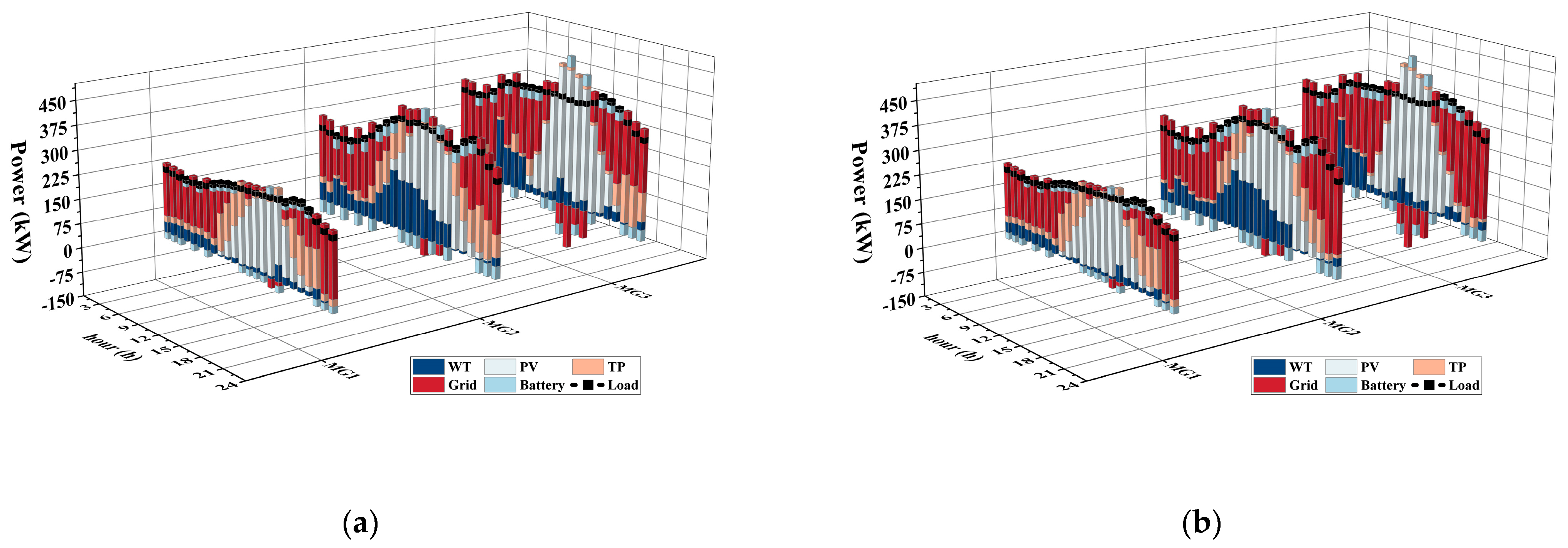
5.3. Analysis of Energy–Carbon Coupling Trading

In order to verify the advantages of the proposed energy–carbon coupling trading method, two scenarios are set based on different operation mechanisms of the MG system in the transition season.

Scenario 6: There is no DNO, and MGs trade directly with the external grid and carbon market.

Scenario 7: The DNO is introduced, and the proposed energy–carbon coupling trading method is considered.

The optimization results of the two scenarios are shown in

Table 5. The optimization results of the energy–carbon coupling trading.

Scenario	Costs of MG 1 (CNY)	Costs of MG 2 (CNY)	Costs of MG 3 (CNY)	Total Costs (CNY)	Profits of DNO (CNY)	CO2 Over-Emissions (kg)
6	3018.9	4096.7	5088.6	12,204.2	/	3216.5
7	3028.8	3871.8	4411.8	11,312.4	37.8	3073.9

.

It can be seen that the total costs and CO₂ over-emissions are reduced after considering the proposed energy–carbon coupling trading method. Compared with Scenario 6, the total costs of MGs in Scenario 7 are reduced by 7.3%. The CO₂ over-emissions in Scenario 7 are 4.4% lower than in Scenario 6. This is mainly because of the lower carbon price than the external carbon market during periods with abundant clean energy output, which reduces the carbon costs of the MGs. In addition, during higher carbon price periods, the MG with surplus CEA can sell itself to reduce operating costs. For the DNO, in the coordination of energy–carbon coupling trading, implementing rational pricing strategies can earn price differentials while also promoting the consumption of clean energy in the networked MG system and reducing overall carbon emissions.

The internal pricing strategy of the DNO is shown in Figure 7, and the dynamic energy flow balance dispatching results of different MGs are shown in Figure 8. Most of the time, the DNO sets its electricity purchase price and sale price to extreme value to guarantee its interests, to stimulate each MG to reduce energy sales and irrational power purchases, and to increase clean energy consumption. From 13:00 to 18:00, the DNO reduces the electricity sale price slightly to encourage the MG to consume excess clean energy output in the MG system, which reduces the carbon emissions of the whole system. From 0:00 to 8:00, the DNO needs to purchase electricity to meet the MGs’ load demand due to the lower output of clean energy units. Therefore, the DNO sets its electricity sale price to the upper limit to ensure it will not lose money. Meanwhile, the DNO increases its purchase price to encourage MG with surplus electricity to sell its electricity.

As for carbon trading, from 12:00 to 18:00, the DNO reduces the carbon price to maintain the price gap, improve the profit, and encourage MGs to consume excess clean energy output with lower carbon emission pressure of electricity purchase. During the peak load period from 19:00 to 22:00, due to the reduction of the clean energy units output, the DNO maintains the carbon price at a high level to stimulate MGs to use less thermal power generation to reduce carbon emissions. Meanwhile, the DNO encourages MGs to adjust the load to the valley period by setting a higher electricity selling price. During the period from 0:00 to 8:00, the DNO further increases the carbon price to avoid MGs excessively increasing electricity consumption during the low electricity price period, which also reduces the carbon emission of the whole MG system.

6. Conclusions

To address the temporal mismatch between the daily scheduling and the yearly CEA, this paper proposes a daily scheduling method for networked microgrids, considering the temporal equilibrium allocation of annual CEA. A carbon emission management framework for networked microgrids is constructed for this method. The conclusions are summarized as follows:

(1)

Compared with the annual averaging allocation of CEA, the proposed temporal decomposition model can better allocate CEA, and a decrease in operating costs and carbon emissions is observed with the same CEA, which verifies the effectiveness of the proposed model.

(2)

The proposed Lyapunov optimization-based low-carbon scheduling model can manage carbon emissions within each dispatch interval and be solved online. The CO₂ over-emissions are reduced by at least 16% and show an excellent long-term economic benefit.

(3)

The overall costs of networked microgrids are reduced by 7.3% through the energy–carbon coupling trading, while the overall CO₂ over-emissions of the MGs are reduced by 4.4%.

However, the seasonal characteristics used in this study represent average values for each season and are based on typical data for the four seasons of the year. While this simplifies the modeling process, we acknowledge that real-world electricity costs and carbon emissions fluctuate significantly across seasons. Future work will incorporate more detailed seasonal data to improve the accuracy of the strategy for the DNO.

References

1. An, I. Special Report on the Impacts of Global Warming of 1.5 C above Pre-Industrial Levels and Related Global Greenhouse Gas Emission Pathways, in the Context of Strengthening the Global Response to the Threat of Climate Change. Sustain. Dev. Efforts Eradicate Poverty 2018, 32. [Google Scholar]
2. Liu, R.; Ding, M.; Wang, S. International net zero emission route and its implications for China’s dual carbon strategy. Reform Strategy 2022, 38, 1–12. [Google Scholar]
3. He, B.; Zheng, H.; Zhang, Q.; Zhao, A.; Tang, H.; Xi, P.; Wei, L.; Li, M.; Guan, Q. Toward a Comprehensive Economic Comparison Framework for Solar Projects: A Case Study of Utility and Residential Scales. Sustainability 2024, 16, 10320. [Google Scholar] [CrossRef]
4. Han, H.; Xu, Y.; Wu, C.; Jiang, X.; Cao, S.; Zang, H.; Chen, S.; Wei, Z. Nash Equilibrium-Based Two-Stage Cooperative Operation Strategy for Multi-Microgrids Considering Uncertainty. Prot. Control Mod. Power Syst. 2024, 9, 42–57. [Google Scholar] [CrossRef]
5. Wang, T.; Huang, Z.; Ying, R.; Valencia-Cabrera, L. A Low-Carbon Operation Optimization Method of ETG-RIES Based on Adaptive Optimization Spiking Neural P Systems. Prot. Control Mod. Power Syst. 2024, 9, 162–177. [Google Scholar] [CrossRef]
6. Vásquez, L.O.P.; Redondo, J.L.; Hervás, J.D.Á.; Ramírez, V.M.; Torres, J.L. Balancing CO2 emissions and economic cost in a microgrid through an energy management system using MPC and multi-objective optimization. Appl. Energy 2023, 347, 120998. [Google Scholar] [CrossRef]
7. Zhong, X.; Zhong, W.; Liu, Y.; Yang, C.; Xie, S. Optimal energy management for multi-energy multi-microgrid networks considering carbon emission limitations. Energy 2022, 246, 123428. [Google Scholar] [CrossRef]
8. Wang, Q.; Wang, H.; Tan, H.; Qi, H.; Li, Z.; Weng, H. Optimization Configuration of Hydrogen Storage in Park Integrated Energy System Considering Photovoltaic Photothermal and Stepped Carbon Trading. South. Power Syst. Technol. 2024, 1–12. [Google Scholar]
9. Qin, M.; Yang, Y.; Zhao, X.; Xu, Q.; Yuan, L. Low-carbon economic multi-objective dispatch of integrated energy system considering the price fluctuation of natural gas and carbon emission accounting. Prot. Control Mod. Power Syst. 2023, 8, 61. [Google Scholar] [CrossRef]
10. Qi, X.; Jiang, Z.; Zhang, J. Low-carbon joint dispatch of integrated energy systems based on differentiated dynamic pricing mechanisms. Int. J. Electr. Power Energy Syst. 2024, 156, 109774. [Google Scholar] [CrossRef]
11. Ma, S.; Mi, Y.; Shi, S.; Li, D.; Xing, H.; Wang, P. Low-carbon economic operation of energy hub integrated with linearization model and nodal energy-carbon price. Energy 2024, 294, 130754. [Google Scholar] [CrossRef]
12. Li, J.; Ge, S.; Liu, H.; Yu, Q.; Zhang, S.; Wang, C.; Gu, C. An electricity and carbon trading mechanism integrated with TSO-DSO-prosumer coordination. Appl. Energy 2024, 356, 122328. [Google Scholar] [CrossRef]
13. Yang, P.; Yang, X.; Yang, L.; Wu, C.; Yang, Z. Low-Carbon Economic Dispatch of Source and Load Based on Carbon Market and Green Certificate Allocation System. South. Power Syst. Technol. 2024, 1–9. [Google Scholar]
14. Feng, H.; Hu, Y.-J.; Li, C.; Wang, H. Rolling horizon optimisation strategy and initial carbon allowance allocation model to reduce carbon emissions in the power industry: Case of China. Energy 2023, 277, 127659. [Google Scholar] [CrossRef]
15. Shi, W.; Li, W.; Qiao, F.; Wang, W.; An, Y.; Zhang, G. An inter-provincial carbon quota study in China based on the contribution of clean energy to carbon reduction. Energy Policy 2023, 182, 113770. [Google Scholar] [CrossRef]
16. Yan, N.; Ma, G.; Li, X.; Guerrero, J.M. Low-carbon economic dispatch method for integrated energy system considering seasonal carbon flow dynamic balance. IEEE Trans. Sustain. Energy 2022, 14, 576–586. [Google Scholar] [CrossRef]
17. Shi, Z.; Yang, Y.; Xu, Q.; Wu, C.; Hua, K. A low-carbon economic dispatch for integrated energy systems with CCUS considering multi-time-scale allocation of carbon allowance. Appl. Energy 2023, 351, 121841. [Google Scholar] [CrossRef]
18. Chen, S.; Shroff, N.B.; Sinha, P. Heterogeneous delay tolerant task scheduling and energy management in the smart grid with renewable energy. IEEE J. Sel. Areas Commun. 2013, 31, 1258–1267. [Google Scholar] [CrossRef]
19. Grillo, S.; Marinelli, M.; Massucco, S.; Silvestro, F. Optimal management strategy of a battery-based storage system to improve renewable energy integration in distribution networks. IEEE Trans. Smart Grid 2012, 3, 950–958. [Google Scholar] [CrossRef]
20. Li, J.; Ge, S.; Xu, Z.; Liu, H.; Li, J.; Wang, C.; Cheng, X. A network-secure peer-to-peer trading framework for electricity-carbon integrated market among local prosumers. Appl. Energy 2023, 335, 120420. [Google Scholar] [CrossRef]
21. Huang, Y.; Wang, Y.; Liu, N. Low-carbon economic dispatch and energy sharing method of multiple Integrated Energy Systems from the perspective of System of Systems. Energy 2022, 244, 122717. [Google Scholar] [CrossRef]
22. Xu, X.; Qiu, Z.; Zhang, T.; Gao, H. Distributed Source-Load-Storage Cooperative Low-Carbon Scheduling Strategy Considering Vehicle-to-Grid Aggregators. J. Mod. Power Syst. Clean Energy 2024, 12, 440–453. [Google Scholar] [CrossRef]
23. Fu, M.; Wu, W.; Tian, L.; Zhen, Z.; Ye, J. Analysis of Emission Reduction Mechanism of High-Tiered Carbon Tax under Green and Low Carbon Behavior. Energies 2023, 16, 7555. [Google Scholar] [CrossRef]
24. Liu, L.; Jiang, K.; Liu, N.; Zhang, Y. Multi-agent Energy-carbon Sharing Mechanism for MGs Based on Stackelberg Game. Proc. CSEE 2024, 44, 2119–2131. [Google Scholar]
25. Cui, X.; Zhao, T.; Wang, J. Allocation of carbon emission quotas in China’s provincial power sector based on entropy method and ZSG-DEA. J. Clean. Prod. 2021, 284, 124683. [Google Scholar] [CrossRef]
26. Yang, M.; Liu, Y. Research on multi-energy collaborative operation optimization of integrated energy system considering carbon trading and demand response. Energy 2023, 283, 129117. [Google Scholar] [CrossRef]
27. Shi, J.; Ye, Z.; Gao, H.O.; Yu, N. Lyapunov optimization in online battery energy storage system control for commercial buildings. IEEE Trans. Smart Grid 2022, 14, 328–340. [Google Scholar] [CrossRef]
28. Neely, M. Stochastic Network Optimization with Application to Communication and Queueing Systems; Springer Nature: Berlin/Heidelberg, Germany, 2022. [Google Scholar]
29. Lakshminarayana, S.; Quek, T.Q.; Poor, H.V. Cooperation and storage tradeoffs in power grids with renewable energy resources. IEEE J. Sel. Areas Commun. 2014, 32, 1386–1397. [Google Scholar] [CrossRef]
30. Xiong, S.; Liu, D.; Chen, Y.; Zhang, Y.; Cai, X. A deep reinforcement learning approach based energy management strategy for home energy system considering the time-of-use price and real-time control of energy storage system. Energy Rep. 2024, 11, 3501–3508. [Google Scholar] [CrossRef]
31. Yang, J.; Wang, Z.; Xu, C.; Wang, D. The Competition Between Taxi Services and On-Demand Ride-Sharing Services: A Service Quality Perspective. Sustainability 2024, 16, 9877. [Google Scholar] [CrossRef]
32. Zhu, P.; Lv, X.; Shao, Q.; Kuang, C.; Chen, W. Optimization of Green Multimodal Transport Schemes Considering Order Consolidation under Uncertainty Conditions. Sustainability 2024, 16, 6704. [Google Scholar] [CrossRef]
33. Liu, D.; Zhang, Y. Research on Location and Routing for Cold Chain Logistics in Health Resorts Considering Carbon Emissions. Sustainability 2024, 16, 6362. [Google Scholar] [CrossRef]
34. Li, Y.; Yang, Y.; Zhang, F.; Li, Y. A Stackelberg game-based approach to load aggregator bidding strategies in electricity spot markets. J. Energy Storage 2024, 95, 112509. [Google Scholar] [CrossRef]
35. Wang, Y.; Liu, Z.; Wang, J.; Du, B.; Qin, Y.; Liu, X.; Liu, L. A Stackelberg game-based approach to transaction optimization for distributed integrated energy system. Energy 2023, 283, 128475. [Google Scholar] [CrossRef]
36. Wang, Y.; Hu, J.; Liu, N. Energy management in integrated energy system using energy–carbon integrated pricing method. IEEE Trans. Sustain. Energy 2023, 14, 1992–2005. [Google Scholar] [CrossRef]
37. Maharjan, S.; Zhu, Q.; Zhang, Y.; Gjessing, S.; Basar, T. Dependable demand response management in the smart grid: A Stackelberg game approach. IEEE Trans. Smart Grid 2013, 4, 120–132. [Google Scholar] [CrossRef]
Figure 1. A framework of the carbon emission management.
Sustainability 16 10986 g001
Figure 2. The framework of the Stackelberg game-based energy–carbon coupling trading.
Sustainability 16 10986 g002
Figure 3. External electricity price.
Sustainability 16 10986 g003
Figure 4. Typical daily output of renewable energy sources, load, and decomposed CEA of MG 1 in four seasons.
Sustainability 16 10986 g004
Figure 5. The dynamic energy flow balance dispatching results of Scenario 2.
Sustainability 16 10986 g005
Figure 6. The dynamic energy flow balance dispatching results of Scenario 3.
Sustainability 16 10986 g006
Figure 7. The internal price optimization result of Scenario 7.
Sustainability 16 10986 g007
Figure 8. The dynamic energy flow balance dispatching results of different scenarios: (a) Scenario 6; (b) Scenario 7.
Sustainability 16 10986 g008